


Languages
Pages
Legal


DUALITY AND APPLICATIONS OF ARRANGEMENTS
PETR FELKELFEL CTU [email protected]://cw.felk.cvut.cz/doku.php/courses/a4m39vg/start
Based on [Berg], [Mount], and [Goswami]
Version from 5.2.2017

Felkel: Computational geometry
(2)
Talk overview
Duality 1. Points and lines2. Line segments 3. Polar duality (different points and lines)4. Convex hull using duality
Applications of duality and arrangements

Felkel: Computational geometry
(3)
1. Duality of lines and points in the plane
Points and lines - both have 2 parameters: – Points – coords x and y– Lines – slope k and y-intercept q
y = kx + q
We can simply map points and lines 1:1 Many mappings exist – it depends on the context
φq k = tg φ

Felkel: Computational geometry
(4)
Why to use duality?
Some reasons why to use duality: Transforming a problem to dual plane may
give a new view on the problem Looking from a different angle may
give the insight needed to solve it Solution in dual space may be even simpler

Felkel: Computational geometry
(5)
Definition of duality transformation D
Let D be the duality transform: Point p = [ px, py ] is transformed
to line Dp = p* := ( b = pxa – py ) Line l : ( y = ax – b ) is transformed
to point Dl = l* := [ a, b ]
pl
x
y
a
b
p*
l*
Primal plane (xy) Dual plane (ab)
variables
constants

Felkel: Computational geometry
(6)
Example and more about duality D
Example: line y = 5x – 3 can be represented as point y*=[5, 3]
Duality D – is its own inverse DDp = p, DDl = l– cannot represent vertical lines
=>Take vertical lines as special cases, use lexico-graphic order, or rotate the problem space slightly.
– Primal plane – plane with coordinates x, y– Dual plane* – plane with coordinates a, b
See the [applet]
Felkel: Computational geometry
(7)
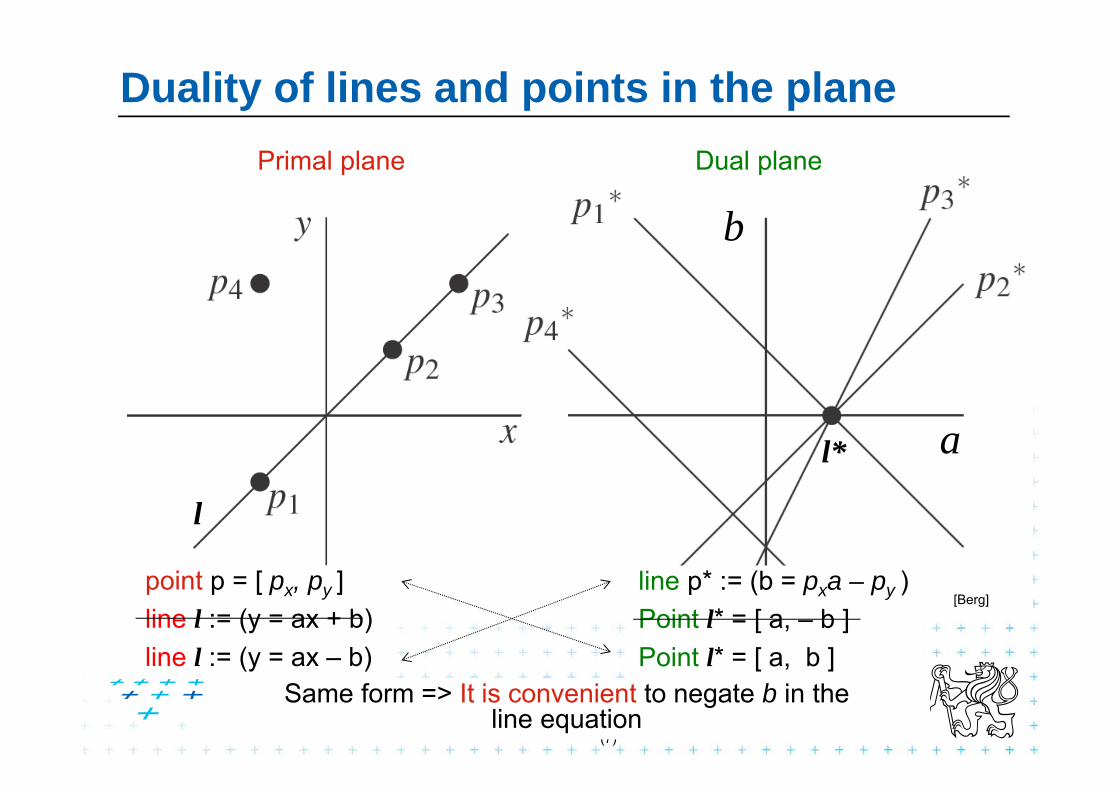
Duality of lines and points in the planePrimal plane Dual plane
a
b
[Berg]
l
l*
point p = [ px, py ]line l := (y = ax + b)line l := (y = ax – b)
line p* := (b = pxa – py )Point l* = [ a, – b ]Point l* = [ a, b ]
Same form => It is convenient to negate b in the line equation
Felkel: Computational geometry
(8)
Why is b negated in the line equation?
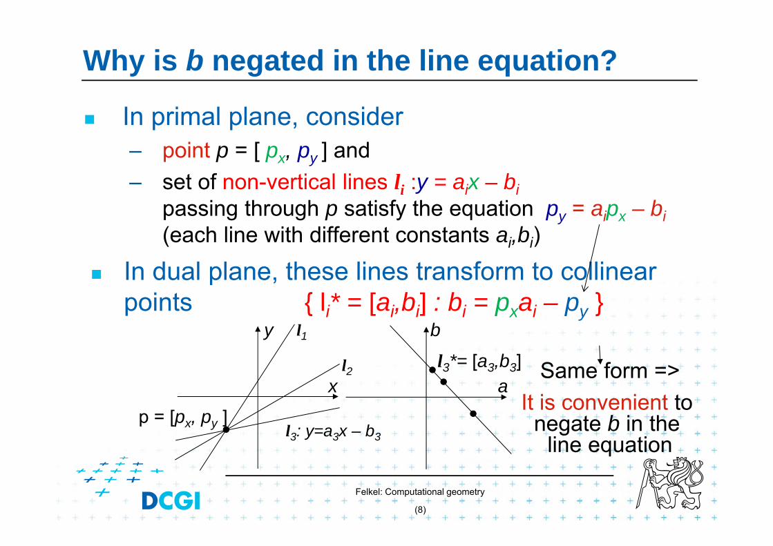
In primal plane, consider – point p = [ px, py ] and – set of non-vertical lines li :y = aix – bi
passing through p satisfy the equation py = aipx – bi(each line with different constants ai,bi)
In dual plane, these lines transform to collinear points { li* = [ai,bi] : bi = pxai – py }
Same form =>It is convenient to
negate b in the line equation
p = [px, py ]
l3*= [a3,b3]a
by
x
l1
l2
l3: y=a3x – b3

If b not negated in the line equation…Lines li have equartion li :y = aix – bi OR y = aix + bi
Passing through point p = [ px, py ] :
With minus– equation li: py = aipx – bi
dual points {li * = [ai,bi] : bi = pxai – py } … same form
With plus– equation li: py = aipx + bi
dual {li * = [ai,bi] : bi = – pxai + py } … different form
Felkel: Computational geometry
(9)
Felkel: Computational geometry
(10)
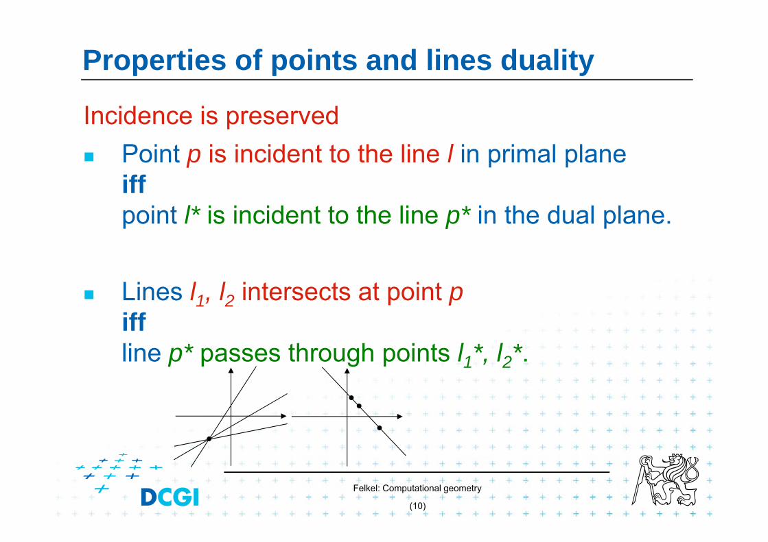
Properties of points and lines duality
Incidence is preserved Point p is incident to the line l in primal plane
iffpoint l* is incident to the line p* in the dual plane.
Lines l1, l2 intersects at point piffline p* passes through points l1*, l2*.
Felkel: Computational geometry
(11)
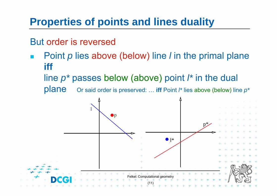
Properties of points and lines duality
But order is reversed Point p lies above (below) line l in the primal plane
iff line p* passes below (above) point l* in the dual plane Or said order is preserved: … iff Point l* lies above (below) line p*
l*
p*

Felkel: Computational geometry
(12)
Properties of points and lines duality
Collinearity Points are collinear in the primal plane iff their
dual lines intersect in a common point
This does not hold for points on vertical line
m*p*
r*
q*p
r
q
m
a
b
x
y

Felkel: Computational geometry
(13)
Dual transform is undefined for vertical lines– Points with the same x coordinate dualize to lines with
the same slope (parallel lines) and therefore – These dual lines do not intersect (as should for collinear points)
– Vertical line through these points does not dualize to an intersection point
– For detection of vertically collinear points use other method - O(n) vertical lines -> O(n2) brute force 3|| lines s.
-> O(n) after O(n log n) sorting by x
Handling of vertical lines
p*q*r*
pq
r Vertical distances of such duals are “preserved”. For px = qx
vertDist(q*b, p*b) = py – qy
a
by
x

Felkel: Computational geometry
(14)
2. Duality of line segments
Line segment s= set of collinear points ––> set of lines passing one point– union of these lines is a (left-right) double wedge s*
p
q
m
s
m*
q*
p*
s*
dual
left
right wedgetop
bottom wedges*
Dvojitý klín

Felkel: Computational geometry
(15)
Line b intersects line segment s – if point b* lays in the double wedge s*,
i.e., between the duals p*,q* of segment endpoints p,q– point p lies above line b and q lies below line b– point b* lies above line p* and b* lies below line q*
p
q
m
s
a
b
cm*
q*
p*
s*
s*
b*
a*
c*
Intersection of line and line segment
Felkel: Computational geometry
(16)
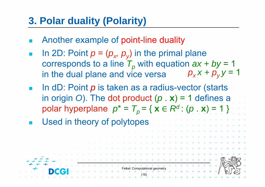
3. Polar duality (Polarity)
Another example of point-line duality In 2D: Point p = (px, py) in the primal plane
corresponds to a line Tp with equation ax + by = 1 in the dual plane and vice versa
In dD: Point p is taken as a radius-vector (starts in origin O). The dot product (p . x) = 1 defines a polar hyperplane p* = Tp = { x Rd : (p . x) = 1 }
Used in theory of polytopes
px x + py y = 1

Felkel: Computational geometry
(17)
Polar duality (Polarity)
Geometrically in 2D, this means that – if d is the distance from the origin(O) to the point p,
the dual Tp of p is the line perpendicular to Op at distance 1/d from O and placed on the other side of O.
[Goswami]
p
1
d
Unit circle
1/d
Tp

Felkel: Computational geometry
(18)
4. Convex hull using duality – definitions
An optimal algorithm Let P be the given set of n points in the plane. Let pa P be the point with smallest x-coordinate Let pd P be the point with largest x-coordinate
Both pa and pd CH(P)Upper hull = CW polygonal chain
pa,…, pd along the hullLower hull = CCW polygonal chain
pa,…, pd along the hull
pa
pd
lower hull
upper hull
Felkel: Computational geometry
(19)
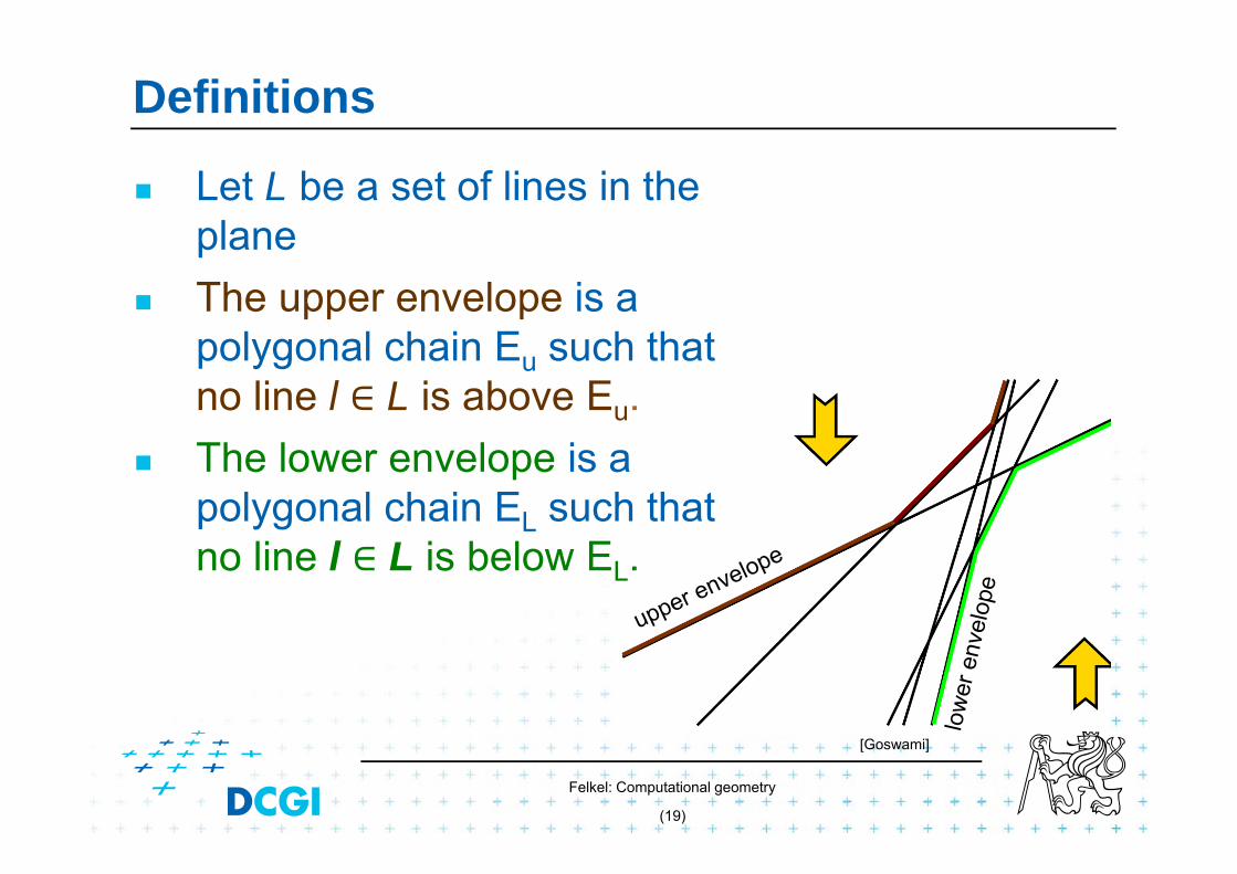
Definitions
Let L be a set of lines in the plane
The upper envelope is a polygonal chain Eu such that no line l L is above Eu.
The lower envelope is a polygonal chain EL such that no line l L is below EL.
[Goswami]

Felkel: Computational geometry
(20)
Connection between Hull and Envelope
ps
lc*
lb*
la*
ps*
ld*
le*
pd
pb
pc
Pa
pe
la
lblc
ldle
ps
p*e
[Goswami]
Felkel: Computational geometry
(21)
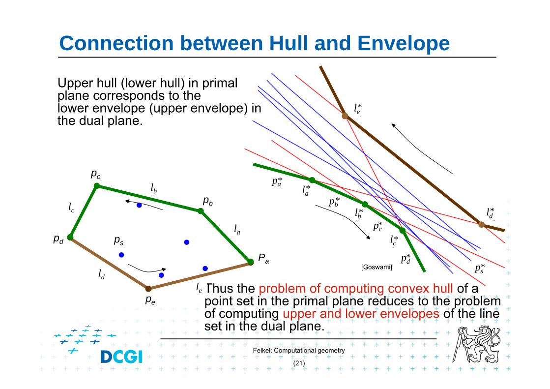
Connection between Hull and Envelope
Upper hull (lower hull) in primal plane corresponds to the lower envelope (upper envelope) in the dual plane.
Thus the problem of computing convex hull of a point set in the primal plane reduces to the problem of computing upper and lower envelopes of the line set in the dual plane.
pd
pb
pc
Pa
pe
la
lblc
ldly
ps
la*
lb*
lc*
ps*
ld*
le*
[Goswami]
la*
lb*
lc*
le
pc*
pa*
pb*
pd*

Input:Output:
UpperEnvelope(L)Set of lines L sorted by increasing order of slopes (-90° to 90°)Polygonal chain O representing the upper hull
1. O = L1 // the only complete line in O2. for i = 2 to n 3. L = last entry in O // O contains half-lines, or line segments,
// except of complete line L14. while( the line segment L does not intersect line Li)5. remove L from O and replace L with its predecessor // L2, L56. insert the line segment Li at the tail of the list O (trim L, trim Li)
Felkel: Computational geometry
(22 / 38)
Upper envelope algorithm
L6
L5
L4
L3
L2L1
L1
L2
L3
L4L5
L6
[Goswami]
Konec animace

Felkel: Computational geometry
(23)
Convex hull via upper and lower envelope
Upper envelope complexity– After sorting n lines by their slopes in O(n logn) time,
the upper envelope can be obtained in O(n) time– Proof: It may check more than one line segment when
inserting a new line, but those ones checked are all removed except the last one.(O(n) insertions, max O(n) removals => O(n) all steps. Average step O(1) amortized time)
Convex hull complexity– Given a set P of n points in the plane, CH(P) can be
computed in O(n log n) time using O(n) space.

Felkel: Computational geometry
(24)
Applications of line arrangement
Examples of applications – solved in O(n2) and O(n2) space by constructing a line arrangement or O(n) space through topological plain sweep.
a) General position test: Given a set of n points in the plane, determine whether any three are collinear.
– Construct an arrangement in dual plane– Report intersections of more than 2 lines
a
b
Felkel: Computational geometry
(25)
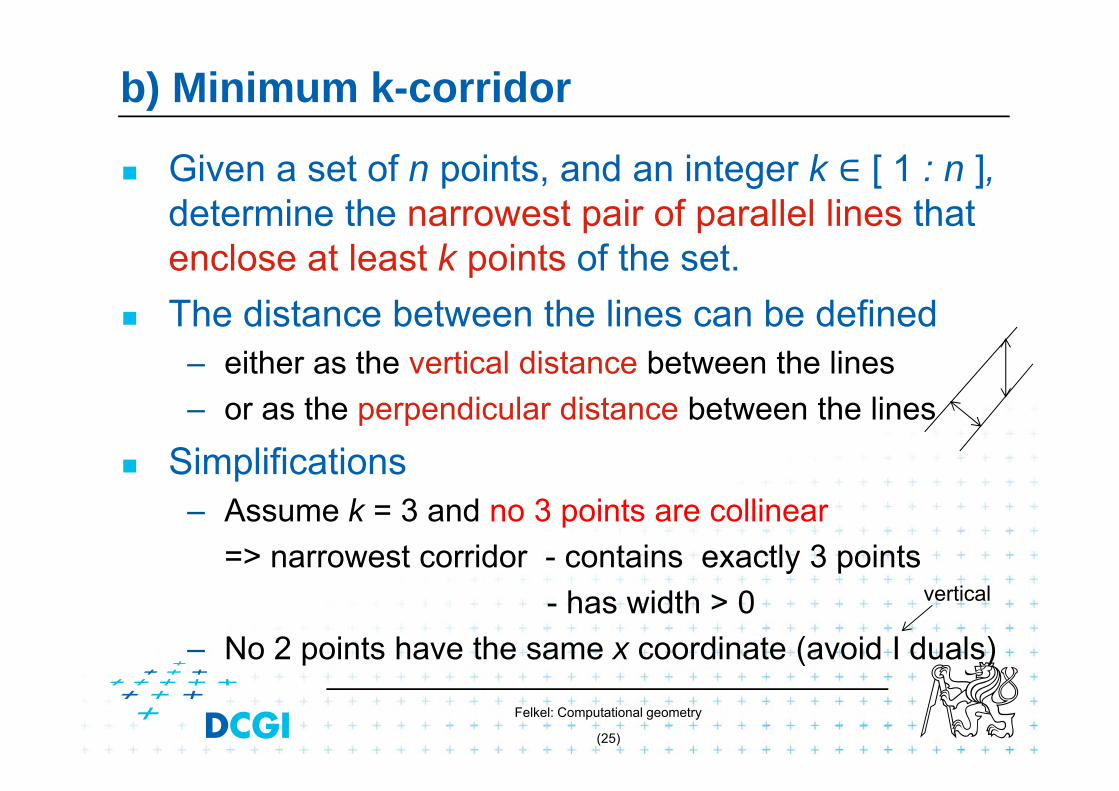
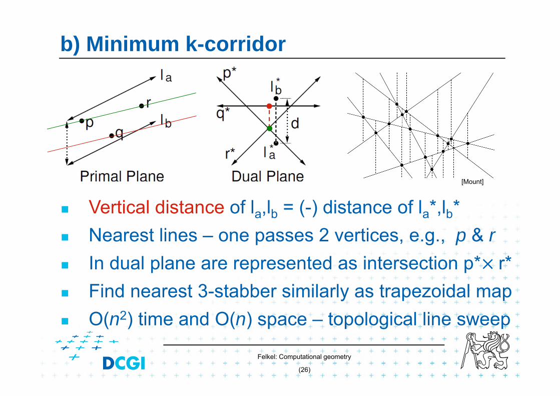
b) Minimum k-corridor
Given a set of n points, and an integer k [ 1 : n ],determine the narrowest pair of parallel lines that enclose at least k points of the set.
The distance between the lines can be defined– either as the vertical distance between the lines – or as the perpendicular distance between the lines
Simplifications– Assume k = 3 and no 3 points are collinear
=> narrowest corridor - contains exactly 3 points- has width > 0
– No 2 points have the same x coordinate (avoid I duals)
vertical
Felkel: Computational geometry
(26)
b) Minimum k-corridor
Vertical distance of la,lb = (-) distance of la*,lb* Nearest lines – one passes 2 vertices, e.g., p & r In dual plane are represented as intersection p* r* Find nearest 3-stabber similarly as trapezoidal map O(n2) time and O(n) space – topological line sweep
[Mount]

Felkel: Computational geometry
(27)
c) Minimum area triangle [Goswami]
Given a set of n points in the plane, determine the minimum area triangle whose vertices are selected from these points
Construct “trapezoids” as in the nearest corridor Minimize perpendicular distances (converted from
vertical) multiplied by the distance from pi to pj
[Goswami]

Felkel: Computational geometry
(28)
Natural application of duality and arrangements Important for visibility graph computation Set of n points in the plane For each point perform an CCW angular sweep Naïve: for each point compute angles to
remaining n – 1 points and sort them => O(n log n) time per point O(n2 log n) time overall Arrangements can get rid of O(log n) factor
d) Sorting all angular sequences – naïve

Felkel: Computational geometry
(29)
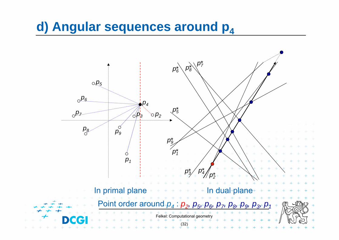
d) Sorting all angular sequences – optimal
For point pi– Dual of point pi is line pi*– Line pi* intersects other dual lines in order of slope
(angles from -90° to 90°) (180°)– We need order of angles around pi
(angles from -90° to 270°) (360°)
– Split points in primal plane by vertical line through pi
– First, report intersections of points right of pi
– Second, report the intersections of points left of pi
– Once the arrangement is constructed:O(n) time for point, O(n2) time for all n points

Felkel: Computational geometry
(30)
d) Angular sequence around p9
p9
p2p3
p4
p5
p6
p7
p8
*p4
*p5
*p6
*p7*p8
*p1
*p2*p3
*p9
p1
In primal plane In dual planePoint order around p9 : p1, p2, p3, p4, p5, p6, p7, p8

Felkel: Computational geometry
(31)
d) Angular sequences around p3
p1
p2p3
p4
p5
p6
p7
p8
*p4
*p5
*p6
*p7*p8
*p1
*p2*p3
p9
*p9
In primal plane In dual planePoint order around p3 : p2, p4, p5, p6, p7, p8, p3, p1
Felkel: Computational geometry
(32)
d) Angular sequences around p4
p1
p2p3
p4
p5
p6
p7
p8
*p4
*p5
*p6
*p7*p8
*p1
*p2*p3
p9
*p9
In primal plane In dual planePoint order around p4 : p2, p5, p6, p7, p8, p9, p3, p1

Felkel: Computational geometry
(33)
e) More applications of line arrangement
Visibility graphGiven a set of n non-intersecting line segments, compute the visibility graph, whose vertices are the endpoints of the segments, and whose edges are pairs of visible endpoints (use angular sequences).
Maximum stabbing line Given a set of n line segments in the plane, compute the line that stabs (intersects) the maximum number of these line segments.

Felkel: Computational geometry
(34)
More applications of line arrangement
Ham-Sandwich cutGiven two sets of points, n red and m blue points compute a single line that simultaneously bisects both setsPrinciple – intersect middle levels of arrangements
Point at k-th level Lk has at most k lines above and at most n – k – 1 lines below
level5
level4
level0 level1
level2level3
[Mount][Goswami]

Felkel: Computational geometry
(35)
References[Berg] Mark de Berg, Otfried Cheong, Marc van Kreveld, Mark Overmars:
Computational Geometry: Algorithms and Applications, Springer-Verlag, 3rd rev. ed. 2008. 386 pages, 370 fig. ISBN: 978-3-540-77973-5, Chapters 8., http://www.cs.uu.nl/geobook/
[Mount] David Mount, - CMSC 754: Computational Geometry, Lecture Notes for Spring 2007, University of Maryland, Lectures 8,15,16,31, and 32.http://www.cs.umd.edu/class/spring2007/cmsc754/lectures.shtml
[applet] Allen K. L. Miu: Duality Demohttp://nms.lcs.mit.edu/~aklmiu/6.838/dual/
[Goswami] Partha P. Goswami: Duality Transformation and its Application to Computational Geometry, University of Calcutta, India http://www.tcs.tifr.res.in/~igga/lectureslides/partha-lec-iisc-jul09.pdf
Top Related