


![Alexis POMPILI ( University & I.N.F.N. of Bari ) [representing the Collaboration]](https://static.fdocuments.us/doc/165x107/56812e08550346895d93730b/alexis-pompili-university-infn-of-bari-representing-the-collaboration.jpg)
Languages
Pages
Legal


Università degli Studi di Roma “La Sapienza”
Dottorato di Ricerca in Ingegneria dei Sistemi
XVII Ciclo
Demand-Assignment Mechanisms in GEO Satellite Systems and Resource-Optimized Algorithms for
Multicast Applications in Wired and Wireless Networks
Relatore Candidato Chiar.mo Prof. Francesco Delli Priscoli Ing. Dario Pompili Coordinatore del Dottorato Chiar.mo Prof. Carlo Bruni
Anno Accademico 2003/2004

Dedico questa tesi a mio padre, mia madre e mia zia, sui quali ho sempre potuto fare affida-
mento, ed alla mia fidanzata Alessandra che con la sua musica tanto mi ha aiutato nel corso di
questi anni di dottorato.
1

ACKNOWLEDGEMENTS
The author wishes to thank most sincerely Prof. Francesco Delli Priscoli for his continuing
guidance in the completion of this work, as well as for his valuable support as advisor during
the entire Ph.D. program.
The author is indebt to his colleagues and friends Ing. Marco Vittucci, Ing. Luca Lopez, Ing.
Giuseppe Sette, and Ing. Gianfranco Santoro for their valuable work offered during the writing
of this manuscript and sound comments that greatly improved the content and readability of this
thesis.
To all the academic members of the System Engineering Department of the University of
Rome “La Sapienza”, I wish to express my deepest gratitude for excellent advice, constructive
criticism, helpful and critical reviews throughout the Ph.D. program.
Prof. Carlo Bruni’s position as a Ph.D. coordinator could not have been filled more ade-
quately.
Last but not least, the author is grateful to the many anonymous reviewers that with their
unselfish comments greatly improved the content of the papers from which this thesis has been
partly extracted.
2
TABLE OF CONTENTS
DEDICATION . . . . . . . . . . . . . . . . . . . . . . . . . . . . . . . . . . . . . . . 1
ACKNOWLEDGEMENTS . . . . . . . . . . . . . . . . . . . . . . . . . . . . . . . . 2
TABLE OF CONTENTS . . . . . . . . . . . . . . . . . . . . . . . . . . . . . . . . . 2
LIST OF TABLES . . . . . . . . . . . . . . . . . . . . . . . . . . . . . . . . . . . . 7
LIST OF FIGURES . . . . . . . . . . . . . . . . . . . . . . . . . . . . . . . . . . . . 8
INTRODUCTION . . . . . . . . . . . . . . . . . . . . . . . . . . . . . . . . . . . . . 11
0.1 First Part . . . . . . . . . . . . . . . . . . . . . . . . . . . . . . . . . . . . .11
0.1.1 Chapter I . . . . . . . . . . . . . . . . . . . . . . . . . . . . . . . . .11
0.1.2 Chapter II . . . . . . . . . . . . . . . . . . . . . . . . . . . . . . . .12
0.2 Second Part . . . . . . . . . . . . . . . . . . . . . . . . . . . . . . . . . . .12
0.2.1 Chapter III . . . . . . . . . . . . . . . . . . . . . . . . . . . . . . . .12
0.3 Third Part . . . . . . . . . . . . . . . . . . . . . . . . . . . . . . . . . . . .13
0.3.1 Chapter IV . . . . . . . . . . . . . . . . . . . . . . . . . . . . . . . .13
0.3.2 Chapter V . . . . . . . . . . . . . . . . . . . . . . . . . . . . . . . .15
0.4 Simulation Software Tools . . . . . . . . . . . . . . . . . . . . . . . . . . . .15
I DEMAND-ASSIGNMENT ALGORITHMS FOR SATELLITE BANDWIDTH AL-LOCATION . . . . . . . . . . . . . . . . . . . . . . . . . . . . . . . . . . . . . . 16
1.1 Introduction . . . . . . . . . . . . . . . . . . . . . . . . . . . . . . . . . . .16
1.2 Basic Definitions and QoS Contract . . . . . . . . . . . . . . . . . . . . . . .19
1.3 Satellite Terminal System Architecture . . . . . . . . . . . . . . . . . . . . .22
1.4 Capacity Demand-Assignment Procedure . . . . . . . . . . . . . . . . . . . .23
1.5 Markov Modulated Poisson Process based algorithm for Satellite Traffic Pre-diction . . . . . . . . . . . . . . . . . . . . . . . . . . . . . . . . . . . . . . 27
1.5.1 Data Generation in a Markov Modulated Poisson Process . . . . . . .28
1.5.2 The Identification/Tuning Phase: the MMPP matching problem . . . .31
1.5.3 The Traffic Prediction Phase . . . . . . . . . . . . . . . . . . . . . .33
1.6 Simulation Results . . . . . . . . . . . . . . . . . . . . . . . . . . . . . . . .33
1.7 Conclusions . . . . . . . . . . . . . . . . . . . . . . . . . . . . . . . . . . .40
II A CONTROL BASED TRAFFIC CONTROLLER PROVIDING QOS GUARAN-TEES . . . . . . . . . . . . . . . . . . . . . . . . . . . . . . . . . . . . . . . . . 42
2.1 Introduction . . . . . . . . . . . . . . . . . . . . . . . . . . . . . . . . . . .42
3

2.2 Traffic Controller Architecture . . . . . . . . . . . . . . . . . . . . . . . . .43
2.3 Main Controller Algorithm . . . . . . . . . . . . . . . . . . . . . . . . . . .45
2.3.1 First Stage: Compliant Bit Rate Assignment . . . . . . . . . . . . . .46
2.3.2 Second Stage: Non Compliant Bit Rate Assignment . . . . . . . . .47
2.4 Simulation Results . . . . . . . . . . . . . . . . . . . . . . . . . . . . . . . .51
2.5 Conclusions . . . . . . . . . . . . . . . . . . . . . . . . . . . . . . . . . . .54
III DIFFSERV-INTEGRATED ALGORITHMS FOR RESOURCE OPTIMIZATIONIN SOURCE SPECIFIC AND GROUP SHARED MULTICAST APPLICATIONSIN INTERNET . . . . . . . . . . . . . . . . . . . . . . . . . . . . . . . . . . . . 55
3.1 Introduction . . . . . . . . . . . . . . . . . . . . . . . . . . . . . . . . . . .55
3.2 DIMRO - DiffServ-Integrated Multicast algorithm for Internet Resource Opti-mization . . . . . . . . . . . . . . . . . . . . . . . . . . . . . . . . . . . . .58
3.2.1 A polynomial time algorithm for the exact determination of channelrates in a multirate multicast . . . . . . . . . . . . . . . . . . . . . .59
3.2.2 Least cost source rooted trees . . . . . . . . . . . . . . . . . . . . .67
3.2.3 DIMRO in non-QoS-aware networks . . . . . . . . . . . . . . . . .67
3.2.4 DIMRO in DiffServ aware networks . . . . . . . . . . . . . . . . . .70
3.3 DIMRO-GS - DiffServ-Integrated Multicast algorithm for Internet ResourceOptimization Group Shared applications . . . . . . . . . . . . . . . . . . . .74
3.3.1 DIMRO-GS in non-QoS aware networks . . . . . . . . . . . . . . .75
3.3.2 DIMRO-GS in DiffServ aware networks . . . . . . . . . . . . . . . .76
3.4 Simulation Results . . . . . . . . . . . . . . . . . . . . . . . . . . . . . . .78
3.4.1 Random network model . . . . . . . . . . . . . . . . . . . . . . . .78
3.4.2 DIMRO Performance Evaluation . . . . . . . . . . . . . . . . . . . .78
3.4.3 DIMRO-GS Performance Evaluation . . . . . . . . . . . . . . . . .82
3.4.4 DiffServ DIMRO and DIMRO-GS Performance Evaluation . . . . . .85
3.5 Conclusions . . . . . . . . . . . . . . . . . . . . . . . . . . . . . . . . . . .90
IV MOBILE AD HOC NETWORKS (MANET) . . . . . . . . . . . . . . . . . . . 91
4.1 The Notion of “Ad Hoc Network” . . . . . . . . . . . . . . . . . . . . . . . . 91
4.2 The Communication Environment and the MANET Model . . . . . . . . . .92
4.3 A Promising Application: “Sensor Networks” . . . . . . . . . . . . . . . . .95
4.4 Mobility Model Introduction . . . . . . . . . . . . . . . . . . . . . . . . . . 98
4.5 Mobility Model Overview . . . . . . . . . . . . . . . . . . . . . . . . . . . . 98
4.6 Cellular Mobility Models . . . . . . . . . . . . . . . . . . . . . . . . . . . .103
4.6.1 Random Walk Mobility Model . . . . . . . . . . . . . . . . . . . . .103
4

4.6.2 Fluid-Flow Mobility Model . . . . . . . . . . . . . . . . . . . . . . .106
4.6.3 Random Gauss-Markov Mobility Model . . . . . . . . . . . . . . . .106
4.7 Ad Hoc Mobility Models . . . . . . . . . . . . . . . . . . . . . . . . . . . .107
4.7.1 Random Mobility Model . . . . . . . . . . . . . . . . . . . . . . . .108
4.7.2 Constant Velocity Random Direction Mobility Model . . . . . . . . .108
4.7.3 Random Waypoint Mobility Model . . . . . . . . . . . . . . . . . . .109
4.7.4 Random Direction Mobility Model . . . . . . . . . . . . . . . . . . .110
4.7.5 A Probabilistic Version of the Random Mobility Model . . . . . . . .111
4.7.6 Smooth Random Mobility Model . . . . . . . . . . . . . . . . . . . .112
4.7.7 City Area, Area Zone, and Street Unit Mobility Models . . . . . . . .113
4.7.8 The Metropolitan, National, and International Mobility Models . . . .115
4.7.9 Group Mobility Models . . . . . . . . . . . . . . . . . . . . . . . . .115
V A PROBABILISTIC PREDICTIVE MULTICAST ALGORITHM IN AD HOCNETWORKS (PPMA) . . . . . . . . . . . . . . . . . . . . . . . . . . . . . . . .129
5.1 Introduction . . . . . . . . . . . . . . . . . . . . . . . . . . . . . . . . . . .129
5.2 Related Work . . . . . . . . . . . . . . . . . . . . . . . . . . . . . . . . . .131
5.2.1 PAST-DM: Progressively Adapted Sub-Tree in Dynamic Mesh . . . .131
5.2.2 ITAMAR: Independent-Tree Ad hoc MulticAst Routing . . . . . . . .132
5.2.3 AODV: Ad hoc On Demand Distance Vector protocol . . . . . . . . .133
5.3 Problem Setup . . . . . . . . . . . . . . . . . . . . . . . . . . . . . . . . . .134
5.3.1 Motivations and Goals . . . . . . . . . . . . . . . . . . . . . . . . .134
5.3.2 Transmission Energy Model . . . . . . . . . . . . . . . . . . . . . .135
5.3.3 Probabilistic Link Cost . . . . . . . . . . . . . . . . . . . . . . . . .135
5.4 Probabilistic Link Cost Function Terms . . . . . . . . . . . . . . . . . . . . .137
5.4.1 Energy Term . . . . . . . . . . . . . . . . . . . . . . . . . . . . . . .137
5.4.2 Distance Term . . . . . . . . . . . . . . . . . . . . . . . . . . . . . .139
5.4.3 Lifetime Term . . . . . . . . . . . . . . . . . . . . . . . . . . . . . .141
5.5 Centralized PPMA . . . . . . . . . . . . . . . . . . . . . . . . . . . . . . . .146
5.5.1 Distance-Based Criterion . . . . . . . . . . . . . . . . . . . . . . . .152
5.5.2 Link Cost-Based Criterion . . . . . . . . . . . . . . . . . . . . . . .154
5.6 Distributed PPMA . . . . . . . . . . . . . . . . . . . . . . . . . . . . . . . .156
5.7 Performance Evaluation . . . . . . . . . . . . . . . . . . . . . . . . . . . . .161
5.7.1 Network Mobility Model . . . . . . . . . . . . . . . . . . . . . . . .162
5.7.2 Simulation Results . . . . . . . . . . . . . . . . . . . . . . . . . . .164
5

5.8 Conclusions . . . . . . . . . . . . . . . . . . . . . . . . . . . . . . . . . . .170
FINAL CONCLUSIONS AND FUTURE RESEARCH . . . . . . . . . . . . . . . . 173
APPENDIX . . . . . . . . . . . . . . . . . . . . . . . . . . . . . . . . . . . . . . . . .176
LIST OF ACRONYMS . . . . . . . . . . . . . . . . . . . . . . . . . . . . . . . . . .178
REFERENCES . . . . . . . . . . . . . . . . . . . . . . . . . . . . . . . . . . . . . . .183
VITA . . . . . . . . . . . . . . . . . . . . . . . . . . . . . . . . . . . . . . . . . . . .194
6

LIST OF TABLES
1 E-mail parameter definitions . . . . . . . . . . . . . . . . . . . . . . . . . . .34
2 File Transfer parameter definitions . . . . . . . . . . . . . . . . . . . . . . . .34
3 Web Browsing parameter definitions . . . . . . . . . . . . . . . . . . . . . . .34
4 Video Conferencing parameter definitions . . . . . . . . . . . . . . . . . . . .35
5 Voice over IP parameter definitions . . . . . . . . . . . . . . . . . . . . . . . .35
6 Shortened variable names . . . . . . . . . . . . . . . . . . . . . . . . . . . . .46
7 IP traffic source statistical parameters . . . . . . . . . . . . . . . . . . . . . .52
8 Average and peak rates of traffic sources . . . . . . . . . . . . . . . . . . . . .52
9 IP packet QoS parameters . . . . . . . . . . . . . . . . . . . . . . . . . . . . .52
10 Network parameters . . . . . . . . . . . . . . . . . . . . . . . . . . . . . . . .78
11 Network node mobility . . . . . . . . . . . . . . . . . . . . . . . . . . . . . .163
12 Simulation parameters . . . . . . . . . . . . . . . . . . . . . . . . . . . . . .164
13 Multicast group size . . . . . . . . . . . . . . . . . . . . . . . . . . . . . . . .164
7

LIST OF FIGURES
1 Downstream and upstream traffic in a Satellite Access Network . . . . . . . . .17
2 Scenario Overview . . . . . . . . . . . . . . . . . . . . . . . . . . . . . . . .18
3 Internal structure of the Satellite Terminal (ST) at timeh . . . . . . . . . . . . 22
4 Example of the proposed capacity assignment procedure (N = 2) . . . . . . . . 25
5 Markov Modulated Poisson Process (MMPP) State Chain . . . . . . . . . . . .29
6 Flow chart of the MMPP prediction algorithm . . . . . . . . . . . . . . . . . .33
7 OPNET Simulation Scenario . . . . . . . . . . . . . . . . . . . . . . . . . . .36
8 Traffic Source parameters and their statistical behaviour . . . . . . . . . . . . .37
9 Queuing delay Cumulative Distribution Functions (CDFs) of Voice (Fig. 9(a))and Video (Fig. 9(b)) IP datagrams . . . . . . . . . . . . . . . . . . . . . . . .38
10 Voice bit loss percentile comparisons expressed for significant capacity values .39
11 Video bit loss percentile comparisons expressed for significant capacity values .39
12 TCP average bit rate comparisons expressed for significant capacity values . . .40
13 SATIP6 reference scenario . . . . . . . . . . . . . . . . . . . . . . . . . . . .43
14 Internal structure of the HS Controller . . . . . . . . . . . . . . . . . . . . . .45
15 Scheme of the control system . . . . . . . . . . . . . . . . . . . . . . . . . . .48
16 PID Controller . . . . . . . . . . . . . . . . . . . . . . . . . . . . . . . . . .50
17 Offered Traffic . . . . . . . . . . . . . . . . . . . . . . . . . . . . . . . . . .53
18 Link Efficiency vs System Congestion . . . . . . . . . . . . . . . . . . . . . .53
19 Determining channel rates:Step 1 . . . . . . . . . . . . . . . . . . . . . . . . 64
20 Determining channel rates:Step 2 . . . . . . . . . . . . . . . . . . . . . . . . 64
21 Determining channel rates:Step 3 . . . . . . . . . . . . . . . . . . . . . . . . 64
22 Determining channel rates:Step 4 . . . . . . . . . . . . . . . . . . . . . . . . 65
23 Determining channel rates:Step 5 . . . . . . . . . . . . . . . . . . . . . . . . 66
24 Correct path computation . . . . . . . . . . . . . . . . . . . . . . . . . . . . .73
25 DIMRO and OSTPRejection Ratein Network 1 . . . . . . . . . . . . . . . . . 80
26 DIMRO and OSTPNetwork Loadin Network 1 . . . . . . . . . . . . . . . . . 80
27 DIMRO and OSTPRejection Ratein Network 2 . . . . . . . . . . . . . . . . . 81
28 DIMRO and OSTPNetwork Loadin Network 2 . . . . . . . . . . . . . . . . . 82
29 DIMRO-GS and FTMRejection Ratein Network 1 . . . . . . . . . . . . . . . 83
30 DIMRO-GS and FTMNetwork Loadin Network 1 . . . . . . . . . . . . . . . 84
31 DIMRO-GS and FTMRejection Ratein Network 2 . . . . . . . . . . . . . . . 84
8

32 DIMRO-GS and FTMNetwork Loadin Network 2 . . . . . . . . . . . . . . . 85
33 DIMRO-GS and FTM average number of link . . . . . . . . . . . . . . . . . .86
34 DIMRO Network Load of DiffServ classes . . . . . . . . . . . . . . . . . . . .87
35 DIMRO-GS Network Load of DiffServ classes . . . . . . . . . . . . . . . . .88
36 DIMRO Lucky Receivers . . . . . . . . . . . . . . . . . . . . . . . . . . . . .89
37 DIMRO-GS Lucky Members . . . . . . . . . . . . . . . . . . . . . . . . . . .89
38 Concept map of mobility models used in simulation and analysis of wirelesscommunication systems . . . . . . . . . . . . . . . . . . . . . . . . . . . . . .99
39 Travelling pattern of a Mobile Node (MN) using the 2-D Random Walk MobilityModel . . . . . . . . . . . . . . . . . . . . . . . . . . . . . . . . . . . . . . .105
40 Travelling pattern of a Mobile Node (MN) using the modified 2-D RandomWalk Mobility Model . . . . . . . . . . . . . . . . . . . . . . . . . . . . . . .105
41 Travelling pattern of a Mobile Node (MN) using the Random Waypoint MobilityModel . . . . . . . . . . . . . . . . . . . . . . . . . . . . . . . . . . . . . . .110
42 Travelling pattern of a Mobile Node (MN) using the Random Direction MobilityModel . . . . . . . . . . . . . . . . . . . . . . . . . . . . . . . . . . . . . . .111
43 Movements of three Mobile Nodes (MNs) using the Column Mobility Model .117
44 Travelling pattern of 12 Mobile Nodes (MNs) using the Column Mobility Model118
45 Travelling pattern of Mobile Nodes (MNs) using the Pursue Mobility Model . .119
46 Travelling pattern of Mobile Nodes (MNs) using the Nomadic Community Mo-bility Model . . . . . . . . . . . . . . . . . . . . . . . . . . . . . . . . . . . .120
47 Reference Point Group Mobility Model . . . . . . . . . . . . . . . . . . . . .121
48 In-Place Mobility Model . . . . . . . . . . . . . . . . . . . . . . . . . . . . .123
49 Overlap Mobility Model . . . . . . . . . . . . . . . . . . . . . . . . . . . . .124
50 Convention Mobility Model . . . . . . . . . . . . . . . . . . . . . . . . . . .124
51 Mobile Nodes represented by their a) Physical Coordinates, and b) Velocities .128
52 Example of thewrongEnergy Term expression in (90) . . . . . . . . . . . . .138
53 Energy Term for different values of the instantaneous power spent in multicastcommunications . . . . . . . . . . . . . . . . . . . . . . . . . . . . . . . . . .140
54 Distance Term for different transmission ranges . . . . . . . . . . . . . . . . .141
55 erf(x) function . . . . . . . . . . . . . . . . . . . . . . . . . . . . . . . . . . .143
56 PDF as in (99) for different distances between the nodes . . . . . . . . . . . .144
57 Lifetime Term for different transmission ranges (Fig. 57(a)), and for differentvalues ofσij (Fig. 57(b)) . . . . . . . . . . . . . . . . . . . . . . . . . . . . .147
58 Centralized PPMA: partition of the potential predecessor setPP(x) . . . . . . 151
59 Centralized PPMA: partition ofPF(x) in PF in(x) andPFout(x) based on the‘distance’criterion (Fig. 59(a)), and based on the‘link cost’ criterion (Fig. 59(b))153
9

60 Distributed PPMA: computation ofcurrent cost andnew cost as in Algorithm 3159
61 Tree lifetime for PPMA and Steiner algorithm for small multicast groups in amediummobility (Fig. 61(a)) andhighmobility environment (Fig. 61(b)) . . .166
62 Tree lifetime for PPMA and Steiner algorithm forlarge multicast groups in amediummobility (Fig. 62(a)) andhighmobility environment (Fig. 62(b)) . . .167
63 Number of connected receivers for PPMA and Steiner algorithm forsmallmul-ticast groups in amediummobility (Fig. 63(a)) andhigh mobility environment(Fig. 63(b)) . . . . . . . . . . . . . . . . . . . . . . . . . . . . . . . . . . . .168
64 Number of connected receivers for PPMA and Steiner algorithm forlarge mul-ticast groups in amediummobility (Fig. 64(a)) andhigh mobility environment(Fig. 64(b)) . . . . . . . . . . . . . . . . . . . . . . . . . . . . . . . . . . . .169
65 Average available node energy for PPMA and Steiner algorithm forsmallmul-ticast groups in amediummobility (Fig. 65(a)) andhigh mobility environment(Fig. 65(b)) . . . . . . . . . . . . . . . . . . . . . . . . . . . . . . . . . . . .171
66 Average available node energy for PPMA and Steiner algorithm forlarge mul-ticast groups in amediummobility (Fig. 66(a)) andhigh mobility environment(Fig. 66(b)) . . . . . . . . . . . . . . . . . . . . . . . . . . . . . . . . . . . .172
10

INTRODUCTION
The present thesis has been developed in the Laboratory of the System Engineering Department
of the University of Rome “La Sapienza”. This thesis presents resource optimized algorithms for
efficient bandwidth sharing in telecommunication systems, and is divided into three parts: the
first part presents demand-assignment mechanisms in GEO (Geostationary Earth Orbit) satellite
systems, while the second and the third part propose resource-optimized algorithms for mul-
ticast applications in wired and wireless networks, respectively. In the following each part of
the thesis, which is composed of one or two chapters, is separately described, and the main
contributions of each chapter is outlined.
0.1 First Part
The first part of this thesis is composed of two chapters, Chapter I and Chapter II, and deals
with the problem of the design of control-predictive based demand-assignment mechanisms for
a satellite network guaranteeing a target QoS (Quality of Service) to Internet traffic, while ef-
ficiently exploiting the air interface. The proposed mechanisms are in charge of dynamically
partitioning the satellite uplink capacity among the connections in progress in the considered
spot-beam. Such a partitioning is performed aiming, on the one hand, to match the QoS require-
ments of each connection and, on the other hand, to maximize bandwidth exploitation.
0.1.1 Chapter I
Chapter I describes a Control Theory approach, based on a Markov Modulated Chain Predic-
tion Model for the traffic forecast, to effectively tackle the problem of the delay between the
bandwidth request and bandwidth assignment, and the signaling overhead caused by control
messages. The presented algorithms efficiently cope with both the satellite propagation delay
and the delays inherent in the periodic nature of the bandwidth demand-assignment mechanism.
The demand-assignment algorithm and the proposed Markov Modulated Chain traffic predic-
tion model are shown to be easy to implement and to improve the overall satellite network
performance.
11

0.1.2 Chapter II
Chapter II presents an innovative control-based Traffic Controller whose objective is to share a
single resource, namely the available bit rate, among a set of IP flows characterized by different
QoS requirements. This Traffic Controller has been developed for a satellite environment, in
the framework of the SATIP6 (SATellite broadband multimedia system for IPv6) project [3]
financed by the European Commission in the context of the 5th framework programme (IST-
Information Society and Technology programme). Nevertheless, the proposed Traffic Controller
can be profitably used in New Generation IP-based Satellites [89] or in any wireless or wired
network. The main novelty behind the proposed Traffic Controller is that it relies on an original
control based approach which exploits a closed-loop architecture and a fuzzy tuner. Simulation
results demonstrated that such Traffic Controller outperforms a well known open-loop Traffic
Controller (namely the one based on the presence of Dual Leaky Buckets and Earliest Deadline
First scheduling algorithm).
0.2 Second Part
The second part of the thesis is composed of Chapter III only.
0.2.1 Chapter III
Chapter III introduces two novel multicast algorithms for wired Internet resource optimization.
The first proposed multicast algorithm, DIMRO (DiffServ-Integrated Multicast algorithm for
Internet Resource Optimization), builds source rooted multicast trees to allow one node in the
multicast group to send data to the other member nodes. This algorithm is suitable for source
specific applications such as live video distribution, software and file distribution, replicated
database server, web site replication, periodic data delivery. The second proposed multicast
algorithm, DIMRO-GS (DiffServ-Integrated Multicast algorithm for Internet Resources Opti-
mization in Group Shared applications), constructs the shared tree connecting each group mem-
ber with all the other group members for group shared applications such as videoconference,
distributed games, file sharing, collaborative groupware, replicated database. The objective is
to achieve efficient traffic balancing in the network in order to avoid bandwidth bottlenecks and
consequent network partitions, which cause low network performance. Both algorithms can be
12

integrated with the Differentiated Service (DiffServ) Quality of Service approach. The QoS ser-
vices requested by the receivers are mapped into the proper DiffServ class, such a way to respect
the expected QoS requirements. The low computational complexity of the proposed algorithms
effectively leads to time and resource saving.
0.3 Third Part
The third and last part of this thesis, which is made up of two chapters, Chapter IV and Chapter
V, proposes efficient multicast algorithms in Ad Hoc Networks.
0.3.1 Chapter IV
Chapter IV describes the main characteristics of Ad Hoc Networks, which are collections of
mobile nodes communicating using wireless media without any fixed infrastructure, as well as
their features and applications. A Mobile Ad Hoc Network (MANET) is a network architec-
ture that can be rapidly deployed without relying on pre-existing fixed network infrastructure.
The nodes in a MANET can dynamically join and leave the network, frequently, often without
warning, and possibly without disruption to other on-going communications. Moreover, the
nodes in the network can be highly mobile. Examples of the use of the MANETs are tactical
operation, for fast establishment of military communication during the deployment of forces
in unknown and hostile terrain; rescue missions, for communication in areas without adequate
wireless coverage; national security, for communication in times of national crisis, where the ex-
isting communication infrastructure is non-operational due to a natural disaster or a global war;
law enforcement, for fast establishment of communication infrastructure during law enforce-
ment operations; commercial use, for setting up communication in exhibitions, conferences,
or sales presentations; education, for operation of wall-free (virtual) classrooms; sensor net-
works, for communication between intelligent sensors mounted on mobile platforms. Nodes in
a MANET exhibit nomadic behavior by freely migrating within some area, dynamically creat-
ing and tearing down associations with other nodes. Groups of nodes that have a common goal
can create formations (clusters) and migrate together, similarly to military units on missions
or to guided tours on excursions. Nodes are equipped with portable communication devices.
Lightweight batteries may power these devices. Limited battery life can impose restrictions
on the transmission range, communication activity (both transmitting and receiving) and com-
putational power of these devices. In addition, all the network nodes have equal capabilities.
13

This means that all nodes are equipped with identical communication devices and are capable
of performing functions from a common set of networking services. However, all nodes do not
necessarily perform the same functions at the same time. In particular, nodes may be assigned
specific functions in the network, and these roles may change over time.
Chapter IV also presents the most popular mobility models used for simulations in ad hoc
networks. The movement pattern of users plays an important role in performance analysis of
mobile and wireless networks. There exists a variety of mobility models that find application
in different kinds of simulations and analytical studies of wireless systems. Cellular mobil-
ity models were developed to test the behavior of cellular protocols and strategies. The most
known cellular mobility model is the Random Walk Model. In the Random Walk Model, a host
moves from its current location to a new location by randomly choosing a direction and speed
in which to travel. In ad hoc wireless mobile networks, the mobility models focus on the in-
dividual motion behavior between mobility ‘epochs’, which are the smallest time periods in a
simulation in which a mobile host moves in a constant direction at a constant speed. A good
mobility model should not change the spatial distribution of the nodes during the simulation.
A property often required for mobility models is to keep uniform that distribution over the en-
tire simulation area. In some mobility model we encounter an unrealistic choppy motion with
sudden stopping, sharp turning, and completely random wandering. A realistic node motion is
another fundamental property a mobility model must have. The most used mobility model in ad
hoc network simulations is the Random Waypoint Mobility Model. In this model, each node of
the network chooses uniformly at random a destination point, i.e., ‘waypoint’, in a rectangular
deployment region. A node moves to this destination with a randomly chosen velocity. When
it reaches the destination, it remains static for a predefined pause time and then starts moving
again according to the same rule. In many situations it is necessary to model the behavior of
mobile nodes that move together. For example, many military scenarios occur where a group of
soldiers must collectively search a particular plot of land in order to destroy land mines, capture
enemy attackers, or simply work together in a cooperative manner to accomplish a common
goal. In order to model such situations, group mobility models exist to account for these new
cooperative characteristics.
14
0.3.2 Chapter V
Chapter V proposes PPMA, a new Probabilistic Predictive Multicast Algorithm in ad hoc net-
works, which leverages the tree delivery structure for multicasting, solving its drawbacks in
terms of lack of robustness and reliability in highly mobile environment. Existing multicast
protocols fall short in a harsh ad hoc mobile environment because node mobility causes conven-
tional multicast trees to rapidly become outdated. The amount of bandwidth resources required
for building up a multicast tree is commonly less than that required for other delivery structures,
since a tree avoids unnecessary duplication of data. However, a tree structure is more subject to
disruption due to link/node failure and node mobility than more meshed structures. This chapter
explores these contrasting issues, and proposes PPMA to solve most of the existing problems
for multicasting in MANETs. By exploiting the non-deterministic nature of ad hoc networks,
the proposed algorithm takes into account the estimated network state evolution in terms of node
residual energy, link availability, and node mobility forecast, in order to maximize the multicast
tree lifetime, and consequently reduce the number of costly tree reconfigurations. PPMA is
provided in both its centralized and distributed version.
0.4 Simulation Software Tools
For all the proposed algorithms this thesis presents performance evaluation through extensive
simulations run on software tools such as OPNET [1] or C++ based simulators. The presented
Integer Linear Problems (ILP), which are used as benchmarks for the performance evaluation
of the developed algorithms, are implemented in AMPL [64] and solved with CPLEX [2].
15

CHAPTER I
DEMAND-ASSIGNMENT ALGORITHMS FOR SATELLITE
BANDWIDTH ALLOCATION
1.1 Introduction
High powered direct broadcast television satellites, using the European DVB (Digital Video
Broadcast) standard, can be used to broadcast high volumes of data directly to home terminals.
At present, these are unidirectional transmission channels that do not allow an interaction be-
tween service providers and users. There are several ways to design a return channel for satellite
broadcast/multicast services. Many believe terrestrial return channels to be the most cost effec-
tive and practical solution. Commonly proposed terrestrial return channels are PSTN, ISDN,
xDSL, GSM/GPRS, etc. However, there is a large world-wide interest for a DVB Return Chan-
nel via Satellite (DVB-RCS) [4], which could be particularly suitable to support a large amount
of non real-time return connections provided that an appropriate bandwidth management mech-
anism is designed (ASTRA BBI system).
In this chapter we propose a dynamic bandwidth management mechanism for an efficient
and flexible partitioning of the uplink capacity available in a given spot-beam among the con-
nections in progress in such spot-beam. This capacity is equal to the sum of the uplink carrier
capacities assigned to such spot-beam. Such a partitioning is performed aiming, on the one
hand, to match the Quality of Service (QoS) requirements of each connection and, on the other
hand, to maximize the bandwidth exploitation. A Control Theory approach, based on a Markov
Modulated Chain Prediction Model for the traffic forecast, is adopted to effectively tackle the
problem of the delay between the bandwidth request and bandwidth assignment, and the sig-
naling overhead caused by control messages [46][45][134]. The proposed mechanism is fully
compliant with the DVB-RCS standard [4]. In the following we will refer to the termdown-
streamandupstreamto indicate the traffic flowing from the Internet to a Satellite Terminal (ST)
and from a ST to the Internet, respectively, as shown in Fig. 1.
In the considered scenario (see Fig. 2), an on-board packet switch is present in charge of
addressing the IP datagrams (hereon referred to as packets) towards a downlink carrier assigned
16
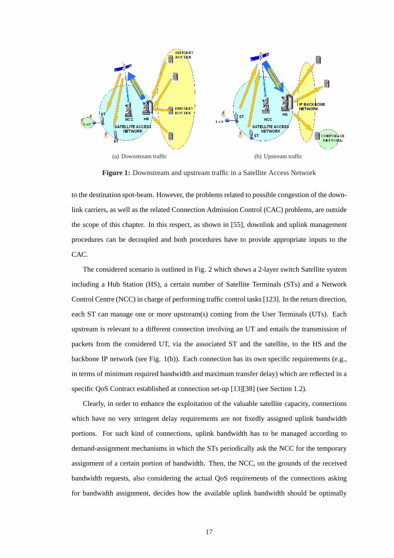
(a) Downstream traffic (b) Upstream traffic
Figure 1: Downstream and upstream traffic in a Satellite Access Network
to the destination spot-beam. However, the problems related to possible congestion of the down-
link carriers, as well as the related Connection Admission Control (CAC) problems, are outside
the scope of this chapter. In this respect, as shown in [55], downlink and uplink management
procedures can be decoupled and both procedures have to provide appropriate inputs to the
CAC.
The considered scenario is outlined in Fig. 2 which shows a 2-layer switch Satellite system
including a Hub Station (HS), a certain number of Satellite Terminals (STs) and a Network
Control Centre (NCC) in charge of performing traffic control tasks [123]. In the return direction,
each ST can manage one or more upstream(s) coming from the User Terminals (UTs). Each
upstream is relevant to a different connection involving an UT and entails the transmission of
packets from the considered UT, via the associated ST and the satellite, to the HS and the
backbone IP network (see Fig. 1(b)). Each connection has its own specific requirements (e.g.,
in terms of minimum required bandwidth and maximum transfer delay) which are reflected in a
specific QoS Contract established at connection set-up [13][38] (see Section 1.2).
Clearly, in order to enhance the exploitation of the valuable satellite capacity, connections
which have no very stringent delay requirements are not fixedly assigned uplink bandwidth
portions. For such kind of connections, uplink bandwidth has to be managed according to
demand-assignment mechanisms in which the STs periodically ask the NCC for the temporary
assignment of a certain portion of bandwidth. Then, the NCC, on the grounds of the received
bandwidth requests, also considering the actual QoS requirements of the connections asking
for bandwidth assignment, decides how the available uplink bandwidth should be optimally
17

Figure 2: Scenario Overview
partitioned, and communicate the relevant decisions to the STs.
A key problem of such a kind of mechanisms relies on the fact that, because of the high
propagation delays of satellite networks, especially for Geostationary Earth Orbit (GEO) satel-
lite [130] where the one-way propagation delay passing through the satellite equals250 ms,
bandwidth assignments are received fractions of second after bandwidth requests (about half a
second in GEO systems).
In addition, in order to keep signaling overhead limited, a certain minimum time interval
must elapse between two consecutive bandwidth requests from the same ST. These issues can
cause further delays in data transfer (which would increase the unavoidable satellite propagation
delay), as well as ST buffer overflows. A possible solution to such problems could be to ask for
more bandwidth than that actually necessary at the time of bandwidth request. Nevertheless, by
so doing, there is the risk of the so-calledover-assignments, i.e., the assignment to a certain ST
of capacity not actually necessary, which, possibly, is subtracted to other STs actually needing
it.
This chapter copes with the above-mentioned problem, by designing an innovative demand-
assignment mechanism and an original traffic prediction model based on a Markov Modulated
Poisson Process (MMPP). The primary objective of these algorithms is, on the one hand, to
18

avoid further delays in data transfer and, on the other hand, to guarantee an efficient exploitation
of uplink satellite bandwidth. Although different works have considered the Demand Assigned
Multiple Access (DAMA) problem [113][93][67], up to the author’s knowledge a few papers
have addressed the demand-assignment problem with QoS guarantees in systems subject to
delays [57][54][52][7][8].
The chapter is organized as follows. Section 1.2 introduces the basic concepts utilized in
the chapter, as well as the objectives of the designed procedures. Section 1.3 presents the Satel-
lite Terminal (ST) architecture. Section 1.4 describes the proposed demand-assignment proce-
dure. Section 1.5 describes the proposed Markov Modulated Poisson Process algorithm which
our demand-assignment procedure is based on for the traffic prediction. Section 1.6 shows
numerical results obtained through extensive simulation campaign run on a satellite simulator
developed with OPNET. Finally, Section 1.7 concludes the chapter sketching the main achieved
results.
1.2 Basic Definitions and QoS Contract
In the following, for the sake of brevity, by “uplink” we always mean the “return uplink”, i.e.,
the link from the ST to the satellite. By “return” traffic (or “return” packets) we indicate the
traffic (or the packets) originated by the UTs and directed to the HS via the STs and the satellite.
Let S denote the number of different STs that are in the considered spot-beam. Leti de-
note a generic ST with at least an in progress connection; so,i can assume the following val-
ues: 1, 2, .., S. Let C(i) denote the number of different uplink connections simultaneously in
progress involving theith ST. Let(i, j) denote a generic in progress uplink connection involving
the ith ST; so,j can assume the following values:1, 2, .., C(i). Practically, the computations
of the various variables will not be performed at any timet, but only at discrete-time instants
th (h = 1, 2, ..) periodically occurring with a proper periodTshort (expressed in seconds), i.e.,
th+1 = th + Tshort. So, in the following, we will just refer to these discrete-time instants and, for
the sake of notation simplicity, the discrete-time instantth will be indicated ash. By hth time
interval, we will mean the time interval[h, h + 1]. Let Rinij (h) denote the bit rate of the return
traffic relevant to the connection(i, j) which, at timeh, is offered to theith ST. Such bit rate is
computed during an appropriate monitoring period according to the following relationship,
Rinij (h) =
∑hk=h−M Lin
ij (k)M · Tshort
(1)
19

where:
M is the duration, expressed in number of discrete-time instants, of the monitoring period
(i.e.,M · Tshort is the monitoring period duration expressed in seconds);
Linij (k) is the sum of the lengths (expressed in bits) of the return packets, relevant to the
connection(i, j), which, during thekth time interval, are incoming into theith ST.
Definition 1 Let Dij denote the queuing delay (expressed in seconds) which a packet relevant
to the connection(i, j) experiences from the time at which it arrives at the ST (coming from an
UT) to the time at which it may be forwarded towards the uplink air interface.
Definition 2 Let Ravij denote the average throughput of a connection(i, j), defined as the ra-
tio between the number of bits transmitted during the connection lifetime and the connection
duration.
The QoS guarantees which have to be granted to a connection are specified in a QoS Contract
[13][38], established at connection set-up. The QoS Contract relevant to the connection(i, j)
includes the following requirements:
1. A first QoS requirement concerns the definition of the traffic to be anyhow granted to the
connection(i, j), i.e., the so-calledStatic Bit Rate, Rstaticij . Note thatRstatic
ij can vary
as time varies. Nevertheless, since these variations are slow with respect to the demand-
assignment procedures dealt with in this chapter, they will not be further considered. An
appropriate Connection Admission Control (CAC) procedure assures that theStatic Bit
Ratesof the in progress connections satisfy the following constraint:
S∑
i=1
C(i)∑
j=1
Rstaticij ≤ Rtot
up (2)
whereRtotup is the overall uplink capacity available in the considered spot-beam.
2. If the connection(i, j) is a Real Time connection (voice, video-conference, etc.), a second
fundamental QoS requirement (hereon referred to asDelay QoS Requirement) concerns
the maximum transfer delay, hereafter indicated asDmaxij , which can be tolerated by the
connection(i, j). This means that, in general, the queuing delayDij should not exceed
Dmaxij . As a matter of fact, in case the queuing delayDij exceedsDmax
ij the packet is
no more meaningful and it is discarded by the ST without being transmitted towards the
20

satellite. In this respect, for Real Time connections a small amount of packet loss can be
tolerated, according to the specific real time application, even though such a loss should
be minimized.
In light of the above, it should be clear that the QoS Contract relevant to a Real Time con-
nection(i, j) is characterized by the two parametersRstaticij andDmax
ij , while the QoS Contract
relevant to a Non Real Time connection(i, j) is characterized by the only parameterRstaticij .
The algorithms proposed in this chapter aim at the minimization of the Real Time traffic to
be discarded because has waited more than the maximum tolerated delay (QoS requirement 2)
and at the maximization of the average throughput of the Non Real Time traffic. In this work
we assume the traffic packet expiration due to theDmaxij overcome as the only possible traffic
loss, meaning that no queue overflows can occur. In other words, we make the assumption that
each queue is dimensioned such a way to accept all possible coming packets. This wayCritical
Traffic will not suffer, under heavy traffic conditions, poor QoS due to queue length exceeding,
as shown in the simulation results.
The ith ST avails of a semi-permanently assignedStatic Bit Rateequal to the sum of the
static bit ratesRstaticij relevant to the connections in progress at such ST. Moreover, it avails of a
Dynamic Bit Ratewhich is temporarily granted by the NCC following the ST requests, according
to an appropriate demand-assignment mechanism (detailed in Section 1.4). LetRdynup denote
the available dynamic uplink capacity defined as the uplink capacity relevant to the considered
spot-beam which is not statically assigned, i.e., the capacity which can be dynamically assigned.
Such a capacity can be easily computed according to the following equation:
Rdynup = Rtot
up −S∑
i=1
C(i)∑
j=1
Rstaticij (3)
Let Rdynij [h1, h2] denote theDynamic Bit Rateassigned to the connection(i, j) during the
time interval [h1, h2]. Clearly, for any time interval[h1, h2], the following uplink capacity
constraint must be respected:
S∑
i=1
C(i)∑
j=1
Rdynij ≤ Rdyn
up ∀h ∈ [h1, h2] (4)
21

Figure 3: Internal structure of the Satellite Terminal (ST) at timeh
1.3 Satellite Terminal System Architecture
Theith ST is provided with a set ofC(i) FIFO Buffers (see Fig. 3): each of these buffers stores
the packets (waiting for being transmitted in the uplink channel) of one of the uplink connections
the ST in question is involved in. A Classifier, which is fed with the traffic coming from the UTs
linked to theith ST, is in charge of sorting the packets towards theC(i) FIFO Buffers. In the
following, for the sake of brevity, the FIFO Buffer storing the packets relevant to the connection
(i, j) will be simply referred to as queue(i, j). Let qij(h) denote the number of bits stored in
the queue(i, j) at timeh. Let δassij [h1, h2] denote the fraction of the available dynamic uplink
capacityRdynup granted by the NCC to the connection(i, j) for being used during the time interval
[h1, h2]. In other words,δassij (h) · Rdyn
up represents theDynamic Bit Rateat which, during the
time interval[h1, h2], theith ST is allowed to forward packets, relevant to the connection(i, j),
towards the uplink air interface. Thus, the parameterδassij [h1, h2] is always included in the range
[0, 1] and, for any time interval[h1, h2], the following fundamental uplink capacity constraint
(which is equivalent to (4)) must be respected:
S∑
i=1
C(i)∑
j=1
δassij (h) ≤ 1 ∀h (5)
22

The packets stored in the queue(i, j) can be either forwarded over the uplink air interface or, if
they are relevant to Real Time connections, discarded because they are expired, i.e., they have
waited more than the maximum tolerated delayDmaxij .
1.4 Capacity Demand-Assignment Procedure
Let us introduce the following definitions (see also Fig. 4):
• Let L denote the round-trip delay expressed in number of time intervals. Such a delay
L is equal to2 · d(Dprop + Tcomput)/Tshorte, whereDprop is the maximum propagation
delay in the run from any ST to the NCC, or in the opposite run, andTcomput is the ST (or
NCC) demand-assignment computing time;
• Let η denote the generic discrete-time at which a ST performs a bandwidth demand; these
times will be referred to asdemand times. In this chapter, for the sake of simplicity, we
assume that all STs synchronously carry out their bandwidth demands, i.e., these demands
are all performed at the same demand times. Moreover, we assume that bandwidth de-
mands are periodically performed. Nevertheless, the concepts can be straightforwardly
extended to the case in which the ST demands are asynchronous and the bandwidth de-
mands are not periodic;
• Let Tinf denote the period occurring between two consecutive bandwidth requests, ex-
pressed in number of time intervals;
• Let N denote the ratio betweenL and Tinf , i.e., N = L/Tinf (for instance, Fig. 4
is relevant to the caseN=2). The choice of the parameterN has to be carried out by
carefully trading-off the contrasting requirements, on the one hand, of frequently sending
the bandwidth requests (thus allowing a tight tracking of the traffic arrived at the STs
coming from the UTs) and, on the other hand, of limiting the signaling overhead caused
by such bandwidth requests. Clearly, the former and the latter requirements drive towards
high and low values for the parameterN , respectively;
• Let Rinij∗[η, h] denote the predictions, performed by theith ST at timeη, of the average bit
rate which will enter the queue(i, j) during thehth time interval (i.e.,Rinij∗[η, h] · Tshort
represent the prediction of the number of bits entering the queue(i, j) during thehth time
23

interval). In Section 1.5, an ad-hoc Markov Modulated Poisson Process (MMPP) predic-
tion model is presented to perform such predictions . This model shows to outperform
other considered prediction models in the simulated scenarios.
In the proposed demand-assignment mechanism the STs do not directly calculate the band-
width they require. Conversely, they just send to the NCC some key parameters which are used
by the NCC itself to perform appropriate bandwidth assignments.
So, whenever at a timeη a bandwidth demand has to be performed, theith ST sends to the
NCC the following pieces of information:
1. TheC(i) predictions of the lengths of the queues(i, j) (j = 1, 2, .., C(i)) at timeη+Tinf ;
at timeη, theith ST computes these predictions, indicated asqij∗(η + Tinf ), according
to the following equation:
qij∗(η+Tinf ) = qij(η)+
η+Tinf−1∑
k=η
Rinij∗[η, k] ·Tshort−δass
ij [η, η+Tinf ] ·Rdynup ·Tinf (6)
2. The C(i) predictions of the average bit rates of the traffic which will enter the queue
(i, j) during the time interval[η + Tinf , η + Tinf + L]; at timeη, the ith ST computes
these predictions, indicated asRinij∗[η + Tinf , η + Tinf + L], according to the following
equation:
Rinij∗[η + Tinf , η + Tinf + L] =
η+Tinf+L−1∑
k=η+Tinf
Rinij∗[η, k]L
(7)
3. TheC(i) coefficientsβij used to grant an higher weight to the queues(i, j) relevant to
Real Time connections which are losing bits because of packet expiries. These coeffi-
cients are computed according to the following expression:
βij = 1 + Kopt · Blossij [η − Tinf , η]
Boutij [η − Tinf , η]
(8)
whereBlossij [η − Tinf , η] represents the amount of bits discarded from the queue(i, j)
during the time interval[η − Tinf , η] due to packet expiries;Boutij [η − Tinf , η] represents
the whole amount of bits that, during the same time interval, is either retrieved from the
queue(i, j) for being forwarded towards the air interface, or discarded from the queue
(i, j) due to packet expiries.Kopt is an appropriate optimized feedback gain whose value
determines the aggressiveness of the feedback control law (the optimal valueKopt=0.97
has been chosen in the simulation experiments reported in Section 1.6).
24

Figure 4: Example of the proposed capacity assignment procedure (N = 2)
Basing on the pieces of information received from the STs, at timeη + L/2, the NCC has
to decide the capacity assignmentsδassij [η + L, η + L + Tinf ] for any (i, j) pair (see Fig. 4).
Then, the proposed idea is to select these assignments aiming at emptying the ST queues at time
η + L + Tinf (this is just the last time at which the assignment decided by the NCC at time
η + L/2 will be effective). The expected length of the queue(i, j) at timeη + L + Tinf can be
computed according to the following equation:
q∗ij(η + L + Tinf ) = q∗ij(η + Tinf ) + Rinij∗[η + Tinf , η + Tinf + L] · L+
−δassij [η + Tinf , η + L] + δass
ij [η + L, η + L + Tinf ] ·Rdynup · L (9)
Note that the termδassij [η + Tinf , η + L] appearing in (9) is relevant to capacity assignments
already performed by the NCC at the time(s) previous toη + L/2. Eq. (9) assumesL > Tinf
which is the most common case. Nevertheless, the extension to the opposite case is straightfor-
ward. Then, thetarget capacity assignments, indicated asδassij
∗[η +L, η +L+Tinf ], which the
NCC, at timeη + L/2, needs to assign in order to empty the ST queues at timeη + L + Tinf ,
can be obtained by imposing that the right hand side of the previous equation is equal to zero,
25

meaning thatq∗ij(η + L + Tinf ) = 0. This yields:
δassij
∗[η + L, η + L + Tinf ] =
q∗ij(η + Tinf )
Rdynup · L
+Rin
ij∗[η + Tinf , η + Tinf + L]
Rdynup
− δassij [η + Tinf , η + L] (10)
However, the target capacity assignment can be actually granted only if the uplink capacity
constraint, expressed in (5), is satisfied. In order to force the respect of this constraint and to take
into account the parametersβij in (8), the actual capacity assignmentsδassij [η +L, η +L+Tinf ]
can be computed according to the following expression:
δassij [η + L, η + L + Tinf ] =
βij · δassij
∗[η + L, η + L + Tinf ]∑S
i=1
∑C(i)j=1 βij · δass
ij∗[η + L, η + L + Tinf ]
(11)
Note that, by using the above-mentioned expression, the uplink capacity constraint is satisfied
with the sign of equality meaning that all the available dynamic uplink capacity is actually
assigned.
In conclusion, the proposed demand-assignment procedure takes place according to the fol-
lowing steps (see also Fig. 4 which assumesN = 2), hereafter described starting from the
generic demand timeη:
1. At the timeη the STs compute the forecast queue lengthsq∗ij(η + Tinf ) according to (6),
the forecast bit ratesRinij∗[η + Tinf , η + Tinf + L] according to (7) and the coefficients
βij according to (8). All these parameters are sent to the NCC.
2. At the timeη+L/2, the NCC receives the pieces of information mentioned in the previous
issue from the STs and, basing on such information, computes, according to (10) and (11),
the capacity assignmentsδassij [η +L, η + L+ Tinf ] to be granted to the connections(i, j)
during the time interval[η + L, η + L + Tinf ]. Such assignments are broadcasted to the
STs.
3. At the timeη +L, theith ST receives the capacity assignmentsδassij [η +L, η +L+Tinf ]
granted by the NCC. These assignments determine the amount of packets which theith
ST is authorized to forward from the queues(i, j) towards the uplink air interface during
the time interval[η + L, η + L + Tinf ]. Moreover, theith ST utilizes these capacity
assignments at next demand time(s) for the computation, according to (6), of the forecast
queue lengths.
26

As a final remark, note that theith ST can rearrange, among the connections(i, j) it is
involved in, the capacity granted to it. In this rearrangement theith ST can take into account
updated information concerning the present lengths of the queues(i, j) (this information was
not available to the NCC when it computed the capacity assignments), according to appropriate
criteria [25][53]. So, at a timeη + L, the ith ST can compute the overall uplink capacity,
indicated asαi[η+L, η+L+Tinf ], assigned to it during the time interval[η+L, η+L+Tinf ],
according to the following equation:
αi[η + L, η + L + Tinf ] =C(i)∑
j=1
δassij [η + L, η + L + Tinf ] (12)
Therefore, the capacities actually granted to the connections during the time interval[η +
L, η + L + Tinf ], δij [η + L, η + L + Tinf ], can differ from the ones granted by the NCC (i.e.,
δassij [η + L, η + L + Tinf ]). Nevertheless, the following constraint must be respected:
αi[η + L, η + L + Tinf ] ≥C(i)∑
j=1
δij [η + L, η + L + Tinf ] (13)
1.5 Markov Modulated Poisson Process based algorithm for SatelliteTraffic Prediction
In this section we introduce our Markov Modulated Poisson Process (MMPP) based algorithm
for satellite traffic prediction. This algorithm is constituted by two phases: 1) theIdentifica-
tion/Tuning phase, and 2) theTraffic Predictionphase. In the Identification/Tuning phase we
find the order of the MMPP chain and the associated parameters according to some aggregated
measurements on the behavior of the IP data stream. More precisely, we will assume ergodicity
of the traffic stream, and we will exchangeTime Averages, which are measured on the traffic
stream, forEnsemble Averages, which are then used to configure the MMPP chain. In the Traffic
Prediction phase we use the tuned MMPP system chain achieve traffic prediction.
The remain of the section is organized as follows. In Section 1.5.1 we recall the main fea-
tures of a Modulated Poisson Process chain and present the general problem of data generation
in this process. In Section 1.5.2 the Identification/Tuning phase is described and the MMPP
matching problem is detailed. Finally, in Section 1.5.3 the Traffic Prediction phase and the
entire MMPP flow chart are presented.
27

1.5.1 Data Generation in a Markov Modulated Poisson Process
A Markov Modulated Poisson Process (MMPP) [46][45][134] of orderNM consists of aNM
state Markov chain in which each statei, (i = 1, 2, .., NM ), is associated to a Poisson process
with rate(λM )i. A MMPP is a time varying Poisson process, whose rate is changed (modulated)
according to the Markov chain. Let us consider in the following a discrete-time Markov chain, as
shown in Fig. 5, which is sampled every∆t, starting from an initial timet0. In the following, for
sake of simplicity, we will use the indexk to represent the discrete-time instanttk = t0 + k∆t.
If Sk (k = 0, 1, ..) is a state moving at discrete-time instants between a finite number of states
i = 1, 2, .., NM with transition probabilities that only depend on the previous state, thenSk
(k = 0, 1, ..) is defined as aMarkov process. Let the matrixP = [pij ] ∈ <NM×NM be the
one-step state transition matrix whose elements are the probabilities to transit from one state
into another in one time-step, as shown in Fig. 5. These are formally defined as:
pij = ProbSk+1 = j | Sk = i, ∀i, j = 1, 2, .., NM (14)
This matrixP can be shown to be astochastic matrixsince it has the property that all its elements
are nonnegative (pij , ∀i, j = 1, 2, .., NM , are probabilities) and that the sum of the elements
in each row equals 1 (each state has at least one possible transition into another state). These
properties can be mathematically expressed as follows:
pij ∈ <+ ∪ 0,NM∑
h=1
pih = 1 ∀i, j = 1, 2, .., NM (15)
Note thatpij do not depend on time, i.e., onk.
Let ΘM (k), at timetk, be the column vector with(ΘM )i(k) = ProbSk = i asith entry,
representing thestate distributionof the chain at stepk. It holds that:
(ΘM )i(k) ∈ <+ ∪ 0,NM∑
i=1
(ΘM )i(k) = 1 ∀k, ∀i = 1, 2, .., NM (16)
Under this assumption, the evolution of a MMPP is completely described by the following
equation:
ΘM (k + 1)T = ΘM (k)T · P (17)
whereT is the transpose operator.
Throughout this chapter, we will neglect thetransitory state, and we will consider the
Markov chain in itssteady state, where the state distributionΘM becomes time-independent,
28

Figure 5: Markov Modulated Poisson Process (MMPP) State Chain
and does not depend anymore on stepk. In the steady state, (17) simplifies to:
ΘMT = ΘM
T · P (18)
It is worth pointing out that the vectorΘM is the left eigenvector of the stochastic matrixPcorresponding to the eigenvalue 1. This is a nonnegative vector and the sum of its elements
equals 1, exactly as in (16), but now without the dependency onk:
(ΘM )i ∈ <+ ∪ 0,NM∑
i=1
(ΘM )i = 1 ∀i = 1, 2, .., NM (19)
Let us introduce theobservationor measurement processψk, (k = 0, 1, 2, ..), which ac-
counts for the incoming IP traffic that we want to predict. In the following we will not represent
traffic according to the fluid approximation, although fluid models1 are widely used in address-
ing a variety of network control problems such as congestion control [114][14], routing [15],
and pricing [156][24]. Rather, we will consider a more realistic model where traffic is actually
made up of discrete-packets of variable length. In our approach, in order to measure traffic,
we logically segment a traffic data stream intofixed-length blocks, whose sizeB is a constant
predefined number of bits. The block sizeB is the finest granularity in the measurement of
traffic and can be as small as needed. This approach allows us to deal with traffic composed
of variable length IP packets, while keeping the complexity of the predicting algorithm low.
This approximation should not been seen as a limiting factor, since we are neither interested in
predicting the packet length nor the inter-arrival time between consecutive packets. In fact, as
explained in Section 1.4, we need to calculateRinij∗[η, h], which is the prediction, performed by
theith ST at timeη, of the average bit rate which will enter the queue(i, j) during thehth time
interval. Thus, we are interested in predicting the average bit rate during a time interval.
1Fluid models replace discrete packets with continuous flows.
29

If we divide the monitoring intervalTmon = K∆t into K sub-intervals each with time-
length∆t, where the maximum number of expected traffic blocks areL, then the following
relation amongB, L, and∆t must hold:
B · L∆t
≥ RinMAX (20)
whereRinMAX is the maximum expected bit rate.
There is a tradeoff between the granularity of the traffic measurement, which depends onB,
and the complexity of the proposed predicting algorithm, which increases asL increases, as will
be clear later on. In particular, the smallerB is, the largerL must be in order to satisfy (20),
given a maximum expected bit rateRinMAX . As far as the choice ofTmon, i.e.,K, is concerned,
the longer the monitoring time is, the more statistically relevant the measures of the traffic are,
but the longer it takes to have updated measures. An appropriate value forTmon should be tuned
considering this tradeoff, as well as the expected statistical variability of the traffic.
Theobservationor measurement processψk, (k = 0, 1, ..), accounts for the number of mea-
sured blocks arriving in the time interval[tk, tk+1]. It has values in the setL : 0, 1, .., L, and
depends probabilistically onSk via the matrixC = [cl+1j ] ∈ <(L+1)×NM , l = 0, 1, .., L, j =
1, 2, .., NM , which represents the Poisson distributions:
cl+1j = Probψk = l | Sk = j =(λM )j
l · e−(λM )j
l!(21)
where(λM )j ≥ 0 is the arrival bit rate of the Poisson process associated with the statej. If
the state parameter(λM )j is 0, then its associated emission bit rate will be zero as well. This
deterministic process will be calledzero process. The row ofC that corresponds to the zero
process is equal to[1 0 · · · 0 ]. LetΞ be the vector withProbψk = l as(l + 1)th entry, then:
Ξ = C ·ΘM (22)
For sake of compactness, the Poisson parameters(λM )i are arranged in a column vectorΛM =
[(λM )i] ∈ <NM . At time stepk, the MMPP, which is described by the tuple〈P; ΛM ; NM 〉, will
generateψk bit emissions according to the Poisson process with arrival rate(λM )i, if the state
of the Markov chain isi. This implies that if(λM )i = 0, no bit emissions will be generated.
In our prediction model we exploit thefirst order statisticsof the bit emissionψk. The
first order statistic is described by the cumulative distribution function, which is defined as
F(v) = Probψk ≤ v, with v = 0, 1, .., L. The MMPP cumulative distribution functionFM
30

is a weighted average of the cumulative distributions of each Poisson process associated to a
state of the chain. Thus:
FM (v) =NM∑
i=1
(ΘM )i · F(λM )i(v) (23)
where
F(λM )i(v) = e−(λM )i ·
v∑
l=0
(λM )il
l!(24)
1.5.2 The Identification/Tuning Phase: the MMPP matching problem
After computing the cumulative distribution function of the arrival processψk, the vectors of the
first order parameters of the MMPP chain,ΛM , ΘM and the model orderNM are determined
by solving anonnegative least squareproblem [100]. When all these first order parameters are
determined, the identification problem is solved, and traffic prediction can be achieved using the
data generation of the determined MMPP chain, as described in Section 1.5.1.
In order to solve the model identification problem, we are concerned with the following
problem: Find NM , ΘM , andΛM , ∀i = 1, 2, .., NM , Givenobservations on the arrivalsψk
for each time stepk = 0, 1, 2, .., K − 1 within the monitoring intervalTmon, so that they form
a MMPP withfirst order statisticsFM matching those of the measured trafficψk, i.e.,Fdata,
as accurately as possible. The state parameter vectorsΘM = (ΘM )i andΛM = (ΛM )i, with
i = 1, 2, .., NM , can then be used to predict future traffic according to (23).
The cumulative distribution function of the data sequence is a staircase function. It is com-
puted as follows:
Fdata(v) =1K·
v∑
j=0
K−1∑
k=0
δ(ψk, j), v = 0, 1, 2, .., L (25)
whereδ(ψk, j) is the Kronecker deltaand K is the total number of subintervals which the
monitoring intervalTmon is divided in.
The distribution function of the MMPP is a linear combination of Poisson distributions, as
can be inferred from (23). The cumulative distribution function of the data,Fdata, must be
approximated by the MMPP cumulative distribution functionFM . This implies thatFdata must
be approximated by anonnegative linear combinationof cumulative distributions of Poisson
processes:
Fd ' D ΘM (26)
31

whereFd is the vector of sizeL+1 with elements(Fd)v = Fdata(v), with v = 0, 1, .., L, andL
is the maximum number of expected traffic blocks. The columns of the matrixD ∈ <(L+1)×NM
correspond to the cumulative distribution functionsF(λM )iin (24).
If the states of the MMPP modeling a given data set were given, i.e., the(λM )i parameters
were known, the matrixD would be determined andΘM could be easily determined by solving
the equations’ system in (26). Without the knowledge of the states or the number of states, which
is a more realistic scenario, the same approach yieldsNM , ΘM andΛM if D is replaced by an
enlarged versionD′ ∈ <(L+1)×N ′M . This matrixD′ has more columns thanD has(N ′
M ≥ NM ),
but the same number of rows. Each column(D′)j , with j = 1, 2, .., N ′M , of this enlarged matrix
represents a possible state, i.e., a possible Poisson cumulative distributions. In fact, in each
subinterval of the monitoring period the domain of possible block arrivals[0, L] is discretized
in order to get a broad choice of candidate states. The discretization step is chosen to increase
linearly because the variance of a Poisson process is equal to its rate. The computed cumulative
distribution vectorFd must be reconstructed as a nonnegative linear combination of the columns
of D′. We can now formulate the optimization problem for the model identification as follows:
P : MMPP Identification Problem
Given : L, N ′M , ψk, k = 0, 1, 2, .., K − 1
Find : x = (x)j ; j = 1, 2, .., N ′M
Min : ‖Fd −D′ x‖2
Subject to : (x)j ≥ 0; j = 1, 2, .., N ′M
(Fd)v = Fdata(v); v = 0, 1, .., L
We solved this problem using theKhun Tucker’s algorithm[126]. The MMPP parameters are
completely defined by the solution of this optimization problem, as follows. Letx∗ be the
optimal value ofx. The number of non-zero components ofx∗ gives automatically the MMPP
model orderNM ≤ N ′M . The indices of the nonzero components ofx∗ represent(λM )j ,
whereas the values of the nonzerox∗ components give(ΘM )j . It worth pointing out the model
orderNM is automatically determined.
32

Figure 6: Flow chart of the MMPP prediction algorithm
1.5.3 The Traffic Prediction Phase
Once the identification problem has been solved, and all the parameters have been tuned, which
are particular tasks characterizing the Identification/Tuning phase, the Traffic Prediction phase
is in charge of predicting the future traffic, according to (23). In Fig. 6, a flow chart of the
entire MMPP algorithm is depicted. It is worth pointing out that each traffic prediction value is
periodically compared to the real incoming data traffic, so that it is possible to know when it is
necessary to trigger a new Tuning phase. To this end, the relative prediction error is constantly
monitored in order to prevent prediction error drift. In fact, if the relative error is higher that a
predetermined threshold, a new identification problem is solved, exploiting the latest available
traffic measurements. This mechanism allows following the dynamics of the input traffic, while
saving precious computational resources.
1.6 Simulation Results
The simulation tool OPNET Modeler 7.0 [1] has been adopted for developing a satellite sim-
ulator and testing the performance of the proposed algorithms. Figure 7 shows the OPNET
simulation scenario, at the network level (a GEO satellite system has been considered for its
33

Table 1: E-mail parameter definitions
Send Interarrival Time [s] exponential (300)Send Group Size1 constant (3)
Email Size (Kbytes) unif int [1,99]Transfer Protocol TCP
Table 2: File Transfer parameter definitions
Inter-Request Time [s] exponential (180)File Size (Kbytes) constant (500)Transfer Protocol TCP
challenging high propagation delay), node level (Satellite Terminals, User Terminals, Hub Sta-
tions, and Network Control Center), and process level (Finite State Machines developed in C-
language which implement the proposed algorithms and the associated protocols). The statis-
tical characteristics of the considered applications are reported in the following tables, and one
statistical realization for each considered traffic source type is sketched in Fig. 8. In particular,
we considered 5 types of applications: 2 Real Time applications, using UDP, namely Voice over
IP and Video-conference, and 3 Non Real Time applications, using TCP, namely FTP, E-mail
and Web browsing [40]. The simulated scenario is the one shown in Fig. 2, which considers a
GEO satellite system(L ≈ 500 ms). The considered spot-beam includes 3 STs. Each of these
STs is connected (e.g., via Ethernet LAN) to 5 User Terminals (UTs). Each of these UTs has 5
connections in progress relevant to the 5 applications listed in the tables, such a way that every
UT is involved in 1 Voice over IP, 1 Video-conference, 1 FTP, 1 E-mail and 1 Web-browsing
connection. This means thatS = 3 andC(i) = 5 (i = 1, 2, 3).
The parametersRstaticij (see Section 1.2) are all set to zero for anyi and anyj. For Real
Time traffic, following the QoS parameters proposed by the ETSI TIPHON project [5], we
have considered the maximum queue delayDmaxij = 50 ms for both Voice over IP and Video-
conference connections (the uplink and downlink GEO propagations alone take about250 ms).
The available uplink capacity in the considered spot-beamRtotup is equal to10 Mbit/s.
Table 3: Web Browsing parameter definitions
HTTP Specification HTTP 1.1Page Interarrival Time [s] exponential (60)
Transfer Protocol TCP
34

Table 4: Video Conferencing parameter definitions
Frame Interarrival Time Information 15 frame/sFrame Size Information (Kbytes) unif int [2,3]
Transfer Protocol UDP
Table 5: Voice over IP parameter definitions
Talk Spurt Length Outgoing2 [s] exponential (0.352)Silence Length Outgoing [s] exponential (0.65)
Encoder Scheme G.711 (Silence)Voice Frames per Packet3 1
Transfer Protocol UDP
Let us point out that all the 95% confidence intervals are not shown in the figures for sake
of clarity.
Figure 9 shows the cumulative distribution of the queuing delayDij experienced by the
packets relevant to Real Time applications, as the parameterN varies. More precisely, Fig. 9(a)
depicts the queuing delay cumulative distribution for the Voice IP datagrams, while Fig. 9(b)
depicts the same metric for the Video IP datagrams. Note that by increasing the value ofN , the
queuing delays are decreased and, in particular, the probability that the queuing delay exceeds
the maximum tolerated delay threshold is also decreased. Nevertheless, we also increase the
signaling overhead. So, as already stressed in Section 1.4,N must be selected by trading off
these contrasting requirements. In addition, Fig. 9 roughly shows thatN = 4 is the lowest
value of N for which we can generally respect the QoS Delay Requirement for Real Time
applications, with an acceptable probability. Thus, this value has been taken in the simulations.
In the following simulations, we compare the performance achieved by using the proposed
capacity assignment procedure, i.e., the procedure described in Section 1.4 (this case will be
hereinafter referred to asall-dynamic) which is deeply based on the Markov Modulated Poisson
Process (MMPP) prediction algorithm in Section 1.5, with the one achieved by fixedly parti-
tioning the available bandwidth among the three STs (this case will be hereinafter referred to as
all-static). Note that in theall-staticcase each ST is fixedly assigned a third of the total available
uplink capacity and no demand-assignment mechanism is required. The simulation parameters
are the same as in the previous simulations, but the available uplink capacityRtotup . As a matter
1Indicates the number of “queued emails” to be sent.2Specifies the time spent by the calling party in speech mode in a speech-silent cycle.3This attribute determines the number of encoded voice frames grouped into a voice packet, before being sent by
the application to the lower layers.
35
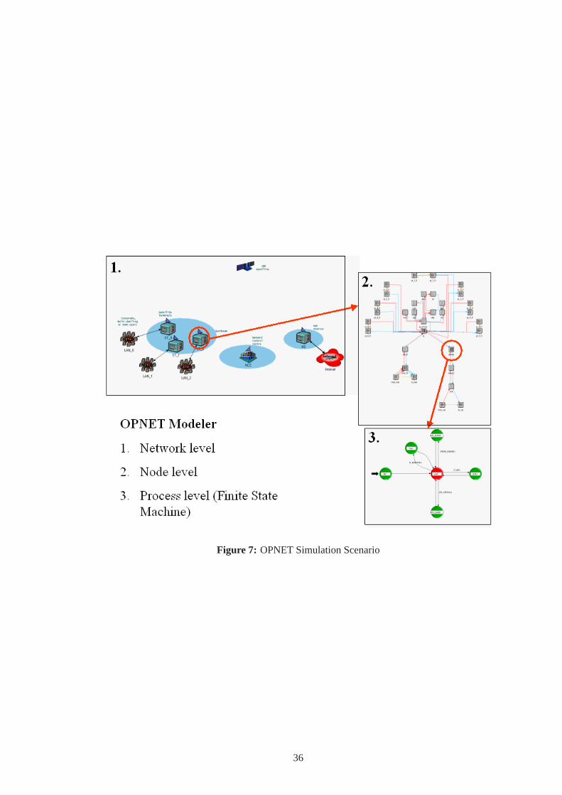
Figure 7: OPNET Simulation Scenario
36

Figure 8: Traffic Source parameters and their statistical behaviour
of fact, we will consider the satellite system behavior when the available uplink capacityRtotup
is varied with respect to anaverage offered uplink capacityof 5.5 Mbit/s defined as the ra-
tio between the total traffic (expressed in bits) offered to the three STs by the UTs during the
simulation time interval and the simulation time interval duration itself. In particular, we con-
sidered three cases in which the available uplink capacity is equal to 80%, 100% and 130% of
the average offered uplink capacity, respectively. In these cases, the following key performance
parameters (corresponding to the targets stated in Section 1.2) are monitored:
• Thebit loss percentileof the Real Time traffic, which is defined as the ratio between the
bits discarded because they have waited more than the maximum tolerated delay, and the
sum of the transmitted and discarded bits;
• Theaverage throughput(see the definition in Section 1.2) of the Non Real Time traffic.
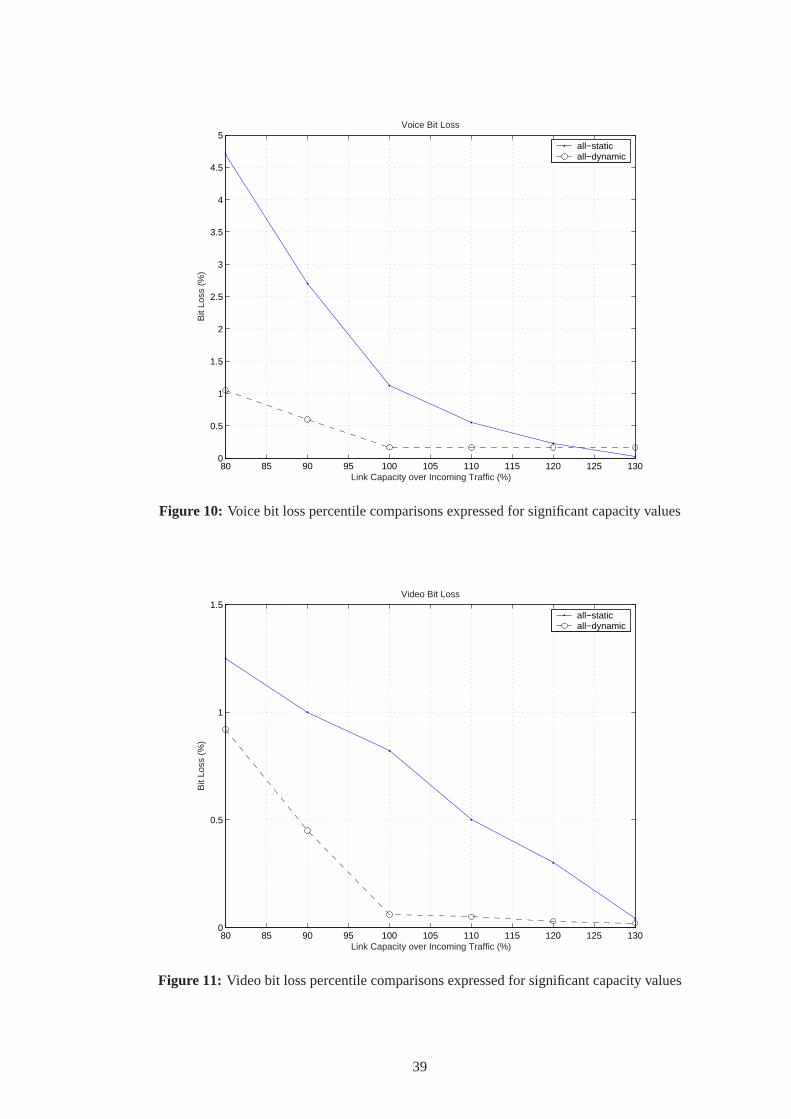
Figure 10 graphs thebit loss percentilefor the Voice over IP application as a function of
the above-mentioned capacity values. The dashed line refers to theall-dynamiccase, while the
solid line to theall-static one. The figure highlights that, if the satellite system is overloaded,
theall-dynamicapproach is remarkably more efficient than theall-staticone, since the proposed
37

(a) Voice
(b) Video
Figure 9: Queuing delay Cumulative Distribution Functions (CDFs) of Voice (Fig. 9(a)) andVideo (Fig. 9(b)) IP datagrams
38
80 85 90 95 100 105 110 115 120 125 1300
0.5
1
1.5
2
2.5
3
3.5
4
4.5
5Voice Bit Loss
Link Capacity over Incoming Traffic (%)
Bit
Loss
(%
)
all−staticall−dynamic
Figure 10: Voice bit loss percentile comparisons expressed for significant capacity values
80 85 90 95 100 105 110 115 120 125 1300
0.5
1
1.5Video Bit Loss
Link Capacity over Incoming Traffic (%)
Bit
Loss
(%
)
all−staticall−dynamic
Figure 11: Video bit loss percentile comparisons expressed for significant capacity values
39

80 85 90 95 100 105 110 115 120 125 130120
130
140
150
160
170
180
190
200
210
220TCP Troughput
Link Capacity over Incoming Traffic (%)
TC
P T
roug
hput
[kbp
s]
all−staticall−dynamic
Figure 12: TCP average bit rate comparisons expressed for significant capacity values
demand-assignment procedure succeeds in exploiting the advantages of statistical multiplexing.
Clearly, as the capacity availability grows, these advantages reduce and for an high capacity
availability, theall-static has a slight advantage over theall-dynamiccase, due to the fact that
the former does not require the demand-assignment procedure (which entails delay and overhead
savings).
Figure 11 is similar to Fig. 10, but refers to the video-conference application. The same
considerations as in Fig. 10 apply. The lower bit loss percentile values obtained for video-
conference depend on the higher maximum tolerated delay of this application with respect to
the voice one.
Finally, Fig. 12 graphs the average throughput for the Non Real Time applications. Once
again, the same considerations as in Fig. 10 apply.
1.7 Conclusions
This chapter dealt with the problem of the design of a control predictive based demand -
assignment algorithm for a satellite network guaranteeing a target Quality of Service (QoS)
to Internet traffic, while efficiently exploiting the air interface. The proposed novel algorithm
40

is in charge of dynamically partitioning the uplink capacity among the connections in progress
in the considered satellite spot-beam. Such a partitioning is performed aiming, on the one
hand, to match the QoS requirements of each connection and, on the other hand, to maximize
bandwidth exploitation. A Control Theory approach, based on a Markov Modulated Chain Pre-
diction Model for the traffic forecast, is adopted to effectively tackle the problem of the delay
between the bandwidth request and bandwidth assignment, and the signaling overhead caused
by control messages. The algorithms efficiently cope with both the satellite propagation delay
and the delays inherent in the periodic nature of the bandwidth demand-assignment mechanism.
The demand-assignment algorithm and the proposed Markov Modulated Chain traffic predic-
tion model are shown to be easy to implement and to improve the overall satellite network
performance. Performance evaluation is carried out by using OPNET network simulator.
41

CHAPTER II
A CONTROL BASED TRAFFIC CONTROLLER PROVIDING
QOS GUARANTEES
2.1 Introduction
One of the main challenges of the out coming telecommunication networks is the provision of
Quality of Service (QoS) guarantees to the IP (Internet Protocol) flows which, most of times,
are currently still served according to a best-effort paradigm which does not assure any QoS
guarantee. The respect of the QoS guarantees, already a challenging goal in wired networks, is
even more challenging in wireless networks in which this goal has to be achieved in conjunction
with an efficient exploitation of the available bandwidth which in wireless networks is a much
more valuable resource than in wired ones. As a result, in wireless networks, traffic control
strategies can be key factors for assuring QoS guarantees and, at the same time, efficiently
exploiting the available bandwidth.
In this respect, this chapter proposes an innovative Traffic Controller which assures an
efficient available bandwidth exploitation while allowing the respect of the QoS guarantees.
This Traffic Controller has been developed for a satellite environment, in the framework of the
SATIP6 (SATellite broadband multimedia system for IPv6) project [3] financed by the Euro-
pean Commission in the context of the 5th framework programme (IST-Information Society
and Technology programme). Nevertheless, the proposed Traffic Controller can be profitably
used in New Generation IP-based Satellites [89] or in any wireless or wired network.
Figure 13 shows the SATIP6 reference scenario [51] where various IP flows coming from
the IP Backbone network arrive at an Hub Station (HS) which is in charge of forwarding them
towards the satellite. The goal is to efficiently share the uplink bandwidth (i.e., bit rate) which
is pre-assigned to the considered HS among the various incoming IP flows meeting the QoS
requirements of these IP flows.
The original adopted approach is based on the presence of a control based Traffic Controller
which continuously computes a parameter providing an updated measurement of the overall
efficiency experienced at the HS, as well as of the efficiencies experienced by each IP flow.
42

Figure 13: SATIP6 reference scenario
Then, appropriate closed-loop control actions steer the single IP flow efficiencies to track the
overall efficiency experienced at the HS. This approach assuresflow fairnessandbandwidth
efficiency, with fairness being defined as the respect of a bandwidth-sharing rule that accounts
for the data flow and time constraints of each connection, which will be explained later on, as
well as thesatisfactionof the QoS guarantees for every IP flow.
The following of the chapter is organized as follows. Section 2.2 presents the Traffic Con-
troller architecture explaining the functions of the various components of such controller. Sec-
tion 2.3 focuses on the Main Controller which is the core of the Traffic Controller since it
includes the control based algorithm which decides the bit rate assignments for each IP flow.
Finally, Section 2.4 shows some meaningful simulation results and Section 5.8 drives some
conclusion.
2.2 Traffic Controller Architecture
The goal of the Traffic Controller is to share the available uplink bandwidth (i.e., the available
uplink bit rate), so as to serve all the accepted IP flows respecting their QoS constraints and
complying with the principles offairnessandefficiency.
As far as the QoS constraints is concerned, the approach which is currently the most widely
used in literature is to identify a set ofQoS Classes[104][34][35]. Many different IP flows can
43

belong to a same QoS Class [118]. A QoS Class is characterized by a set of QoS guarantees
[38][5] (hereafter, also refereed to asQoS contract), namely:
1. A minimum bit rate, hereafter referred to asCompliant Bit Rate, which must be granted
to the IP flows belonging to the QoS Class in question in whichever traffic condition;
2. A maximum (hereafter indicated asDmax) and a minimum (hereafter indicated asDmin)
transfer delay which must be experienced by the IP packets belonging to the IP flows in
question.
Note that the constraint on the maximum tolerated transfer delay comes from the obvious re-
quirement of guaranteeing IP packet delivery within given delays, while the constraint on the
minimum transfer delay comes from the requirement of limiting the delay jitter (whose maximal
value is indicated hereafter asJmax=Dmax-Dmin).
Each IP flow is associated to a QoS Class by setting a proper field of the header of all IP
packets belonging to the IP flow in question to the value corresponding to the selected QoS
Class. This means that all the IP packets relevant to IP flows belonging to a same QoS Class
have the above-mentioned IP packet header field set to the same value.
The internal structure of the HS Traffic Controller is shown in Fig. 14. The IP packets
coming from the Internet, i.e., theOffered Traffic, are sorted into a set of FIFO (First in First
out) Queues. A one-to-one association between queues and QoS Classes exists: each IP packet
is enqueued into the FIFO Queue associated to the QoS Class the IP packet in question belongs
to.
The core of the Traffic Controller is the Main Controller which takes the decisions concern-
ing the IP packets to be retrieved from the FIFO (First Input First Output) Queues for being
forwarded towards the air interface (i.e., towards the satellite). The Main Controller takes its
decisions basing on the following parameters, which are monitored everyTcontrol seconds (here-
after referred to asControl Period):
1. TheQueue Lengthsof the FIFO Queues;
2. TheDiscarded Bit Rates, i.e., the bit rates of the traffic which has to be ruled out by the
various FIFO Queues;
3. TheTransmitted Bit Rates, i.e., the bit rates of the traffic which is retrieved from the FIFO
Queues for being transmitted towards the satellite through the physical interface.
44

Figure 14: Internal structure of the HS Controller
Periodically, everyControl Period, the Main Controller, basing on these three parameters
and taking into account theCompliant Bit Rate, computes theAssigned Bit Rates, i.e., the bit
rates which can be granted to the various IP flows in the nextControl Period. TheAssigned Bit
Ratesare expressed as fractions of theTotal HS Bit Rate, i.e., the bit rate which is currently as-
signed to the considered HS. TheAssigned Bit Ratesare communicated by the Main Controller
to the Scheduler, which is in charge of retrieving from the FIFO Queues the IP packets to be
forwarded towards the satellite, trying to comply the bit rate assignments decided by the Main
Controller.
Note that the Main Controller assumes a continuous-flow model of the inbound traffic, i.e.,
it bases its computations on continuous measures of bit rates and bit lengths, overlooking the
discrete nature of the IP packet flows, while the Scheduler takes into account the discrete nature
of the IP packets. This causes a certain difference between the bit rates actually assigned to the
IP flows and the ones decided by the Main Scheduler. In this respect, the Scheduler implements
a proper bit credit system [56] which aims at keeping close to zero the error between the bit
rates actually assigned to the IP flows and the ones decided by the Main Controller.
It is important remarking that the IP packets which have waited in the FIFO Queues more
than their maximum tolerated transfer delayDmax are discarded (i.e., are lost).
2.3 Main Controller Algorithm
As stated in the previous section, the control action performed by the Main Controller takes
place at the beginning of everyControl Period, namely everyTcontrol seconds. Conceptually,
45

Table 6: Shortened variable names
Parameter Shorted variableQueueLengthi QLeni
OfferedRatei OffRi
TransmittedRatei TransmRi
LossRatei LossRi
CompliantRatei ComplRi
TotalHSRate TotalHSR
SpareHSRate SpareHSR
CompliantAssignedRatei ComplAsRi
NonCompliantAssignedRatei NComplAsRi
AssignedRatei AsRi
FlowEfficiencyi FlowEffi
HSEfficiency HSEff
∆Efficiencyi ∆Effi
∆Ratei ∆Ri
∆AssignedRatei ∆AsRi
FlowAssignedRatei FlowAsi
Priorityi Pri
HSPriority HSPr
the control action consists of two stages:
1. The assignment of theCompliant Bit Rates,
2. The assignment of theNon Compliant Bit Rates.
In the first stage (detailed in Section 2.3.1) the Main Controller assigns a part of theTotal
HS Bit Rateto the IP flows according to theirCompliant Bit Rates; then, in the second stage,
(detailed in Section B) the Main Controller assigns the remaining part of theTotal HS Bit Rate
according to the algorithm described in the following. The sum of the two above-mentioned
assigned values for the i-th IP flow will be hereafter referred to asAssignedRi, whose value
will be used throughout the whole followingControl Period.
In the following, the various parameters of interest will be referred to the i-th flow and to
theControl Periodand will be indicated with self-explaining name, as shown in Tab. 6.
2.3.1 First Stage: Compliant Bit Rate Assignment
In the first stage of the control action the Main Controller checks theOfferedRatei of the i-th
IP flow (i.e., the average bit rate offered by the IP flow in the lastControl Period) and compares
this value with the itsCompliant Bit Rate, granting to the i-th IP flow aComplAssignRatei
46

equal to the lower of the two values (so as to comply with the QoS contract, while avoiding
waste of bandwidth).
The rationale behind this choice is to assign output bit rate on the base of the input (of-
fered) bit rate. Then, the Main Controller computes theSpareHSRate, which is equal to the
TotalHSRate minus the sum of all theCompliant AssignedRatei; note that this value is
always positive since the sum of theCompliant Bit Ratesis always less than theTotalHSRate,
as guaranteed by a proper IP flow admission control mechanism [52][53][54].
In the second stage, theSpareHSRate has to be partitioned into theNon Compliant
Assigned Ratei according to the algorithm detailed in the following section. Clearly, for every
IP flow i theAssigned Ratei is equal to the sum of theCompliant Assigned Ratei plus the
Non Compliant Assigned Ratei.
2.3.2 Second Stage: Non Compliant Bit Rate Assignment
This second stage is the core of the control action and the main novelty of this work. The
approach used by the Main Controller in order to assign theSpareHSRate to the IP flows is
based on the concept of comparing the status of each IP flow with the overall HS status and
of increasing or decreasing the assignment aiming at assuring an uniform handling of every
connection. Figure 15 shows the overall control scheme this second stage is based on, under the
assumption that the considered HS is handlingN IP flows.
For the sake of clarity, the algorithm behind this control scheme is split in three steps detailed
in Sections 2.3.2.1, 2.3.2.2, and 2.3.2.3, respectively.
2.3.2.1 Computation of Priority and Efficiency of the single IP flows
The first step of the algorithm is the definition of a parameter, indicated asPriority (Pri),
which takes into account the current“need for bandwidth”of every i-th connection
Pri =QLeni
Tcontrol+ TransmRi + LossRi (27)
Note that if both members of Equation 27 were multiplied byTcontrol, the left part of the equa-
tion (Pri · Tcontrol) would be equal to the sum of the current number of bits in the queue
associated to the i-th IP flow (QLeni), plus the number of bits that have been transmitted
(TransmRi · Tcontrol) and the number of those that have been discarded (LossRi · Tcontrol) in
theControl Period. In other words,Pri · Tcontrol represents the total number of bits that would
47

Figure 15: Scheme of the control system
be stored in an ideal queue, if all the arrived bits were enqueued doing neither transmissions nor
discards for all the length of theControl Period.
Then, we introduce the parameterFlowEfficiencyi as:
FlowEffi =
AsRi
Pri(28)
High values ofFlowEffi mean that the bit rate assigned to the i-th IP flow is consistent with its
actual need for bandwidth, expressed byPriorityi and vice versa. This ratio is performed by
the component named“Normalizer” in Fig. 15. In fact it normalizes the bit rate assigned to an
IP flow taking into account itsPriority.
2.3.2.2 Computation of Priority and Efficiency of the overall HS
In this second step of the algorithm we extend the approach behind the parametersPriorityi and
FlowEffi to the overall HS, in order to achieve overall HS parameters which can be compared
with the ones associated to the single IP flows. To do this, we introduce two other metrics, the
48

HSPriority and theHSEff , defined as follows:
HSPr =N∑
i=1
Pri (29)
HSEff =TotalHSR
HSPr(30)
All the computations relevant to the first and the second steps are performed by the component
named “Averager” appearing in Fig. 15.
2.3.2.3 Closed-loop computation of theAssignedRatei
The basic idea behind our Controller is to compute the efficiency of each IP flow and to compare
it with the HS overall efficiency: the difference is used to assess whether to increase or to
decrease the bandwidth assigned to the i-th IP flow.
Referring to the i-th IP flow, the algorithm computes, in a closed-loop fashion, theAssigned
Ratei (i.e., the total bit rate that the i-th IP flow will be assigned in the nextControl Period)
with the following five step procedure:
1. HSEff andFlowEffi are compared in order to assess if the i-th IP flow is under-served
or over-served. The difference between the two above-mentioned parameters is the so-
called∆Effi : positive values of this parameter mean that the i-th IP flow is under-served
so that its efficiency must be increased, and vice versa;
2. ∆Effi is multiplied byPriorityi to obtain∆Ratei, which represents the bit rate assign-
ment variation which will align the i-th IP flow efficiency with the overall HS efficiency;
3. ∆Ratei is fed to a PID (Proportional-Integral-Derivative) Controller whose parameters
are controlled by a Fuzzy Tuner (see Figure 16), as detailed in section 2.3.2.4. The result
is ∆AssignRatei;
4. ∆AssignedRatei is summed to theNonCompliantAssignedRatei computed in the
previousControl Period;
5. After a precautional non-linear resharing aiming at avoiding negative values of theNon
Compliant Assigned Ratei (that could decrease theCompliant Assigned Ratei and
cause the infringement of the QoS contract relevant to the i-th IP flow), theNon Compliant
Assigned Ratei is summed to theCompliant Assigned Ratei, thus obtaining the
Assigned Ratei.
49

Figure 16: PID Controller
2.3.2.4 PID control and Fuzzy tuning
Figure 16 shows the selected PID Controller whose parameters are controlled by a Fuzzy Tuner.
This element implements three different sets of rules, relevant toProportional, Integral and
Derivative Actions, as detailed in the following.
Proportional Action: the first set of rules concerns the tuning of the PID Controller ag-
gressiveness which is regulated by theKPi parameter. The various IP flows strive to obtain a
common and limited bandwidth: when there are many flows with respect to the available band-
width many of them may be under-served; this would cause high requests of bandwidth from
most of the current active flows, resulting in the risk of oscillation and instability. The system
manages to reach stability by reducing the aggressiveness of the PID Controller.
In order to defineCongestionwe introduce the following two parameters:NeedandSurplus.
The former represents the cumulative request for bandwidth of all the flows that are under-served
while the latter represents the cumulative bandwidth of the flows that are over-served, i.e.,:
Need =N∑
i=1
max[∆AssignRatei ; 0] (31)
Surplus =N∑
i=1
max[−∆AssignRatei ; 0] (32)
By adopting the two above-mentioned metrics, i.e., (31) and (32),Congestion, a new metric to
evaluate the traffic load, can be defined as follows:
Congestion =Need
Need + Surplus(33)
In the following we exploit thefuzzy1 logic in order to control the PID parameters. The basic
1“What is striking is that its most important and visible application today is in a realm not anticipated when fuzzylogic was conceived, namely, the realm of fuzzy-logic-based process control”[159].
50

idea of “Fuzzy Logic Control” (FLC) was suggested in [157][158]. FLC provides a nonanalytic
alternative to the classical analytic control theory. By utilizing simple triangular fuzzy sets
[88] and the Sugeno deduction [145], we implemented three rules in order to decreaseKPi
asCongestionincreases, and to decreaseKIi andKD
i as∆Effi decreases. This rule prevents
newly established IP flows from pulling pre-existing IP flows away from the equilibrium - as
these flows have null assigned bit rate, their priority is very high at the moment of inception
and may tend to overcome other requests. This phenomenon is not usually present for bursty
sources, as they have some cumulated assigned bit rate.
IntegrativeandDerivative Actions: the second and third fuzzy rules control the parameters
KIi andKD
i according to the usual principles of PID tuning [17][18][19]. Note that the tuning
of these last two parameters is tailored on each IP flow.
As far as theIntegrative Actionis concerned, it is used to speed up the control when the
system is distant from equilibrium, and to turn off it when the equilibrium is approached. In
particular, this action is useful in the transients when the FIFO Queues fill up: the approximately
linear increase of the queue length - bit rates from bursty sources (FTP, Web-browsing) can be
considered almost constant during a burst, and bit rates from stable sources (Voice, Video) have
a little variance around their mean value and can be considered, again, almost constant - causes
a decrease in thePriorityi of the i-th flow that is almost linear (in a Taylor series), properly
controlled by an integrator component.
As far as theDerivative Actionis concerned, our simulations prove that it introduces minor
benefits to the overall system performance.
2.4 Simulation Results
The overall control scheme has been simulated by using the discrete event OPNET [1] simulator
by MIL3. We have compared its performance with the one of some popular scheduling schemes.
We have considered four QoS Classes: Voice, FTP, Video, Web-browsing.
Figure 17 graphs, on a ten minute time-span which allows to have small 95% confidential
intervals, the Offered Bit Rates of one IP flow for each of the four considered QoS Classes. The
statistical parameters characterizing these IP flows are reported in Tab. 7 while in Tab. 8 the
average and peak rate for each traffic application are shown.
Table 9 reports the parameters characterizing the QoS contract of the four considered QoS
51

Table 7: IP traffic source statistical parameters
Datagram length (bits) Interval times (ms)Voice Const.580 Const.20FTP Unif. [320,39680] Unif. [50,150]Web Unif. [320,23680] Unif. [50,550]Video Unif. [320,23680] Gauss.avg.=8.1,σ=4.5
Table 8: Average and peak rates of traffic sources
Ravg.(Kbps) Rmax(Kbps)Voice 29 29FTP 200 400Web 40 240Video 1350 1460
Classes.
The performance achieved by the proposed Competitive Access Controller, are compared
with the one of a FIFO Controller and of an Open-Loop Controller detailed in the following.
In the FIFO Controller only one queue is considered: all the IP packets are enqueued in
this queue and are served according to a First In First Out (FIFO) discipline without taking into
account the QoS requirements of the IP flows.
In the Open-Loop Controller[128] the incoming IP traffic is sorted, according to its QoS
Class, to a set of DLBs (Dual Leaky Buckets) [38] which are used to identify the Compliant
traffic which is served, on a first priority basis, according to an Earliest Deadline First (EDF)
algorithm [108]; the Non Compliant traffic is served, on a second priority basis, again according
to an EDF algorithm. The name of the scheduling controller is due to the fact that DLB parame-
ters are statically set without any closed loop mechanism. Open loop refers to the fact that once
schedules are created they are not “adjusted” based on continuous feedback. While open-loop
scheduling algorithms can perform well in static or dynamic systems in which the workloads can
be accurately modeled [78], they generally perform poorly in unpredictable dynamic systems,
as it is shown in this section.
Table 9: IP packet QoS parameters
Dmax(s) Dmin(s) Jmax(s)Voice 0.1 0.01 0.09FTP 4 0.2 3.8Web 1.5 0.05 1.45Video 0.5 0.02 0.48
52
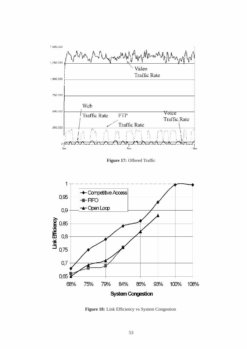
Figure 17: Offered Traffic
Figure 18: Link Efficiency vs System Congestion
53

Figure 18 graphs the Link Efficiency (i.e., the link exploitation) of the considered con-
trollers as a function ofSystem Congestion, this metric being defined as the ratio between the
TotalHSBitRate and the average bit rates of the overall offered traffic. For the Competitive
Access Controller, the QoS constraints are never infringed and the IP packet loss is close to zero
even for aSystem Congestionclose to 98%. As can be seen in Figure 18, the Competitive Ac-
cess Controller outperforms the other controllers (in each load condition) and manages to obtain
near ideal performance with aLink Efficiencywhich closely follows theSystem Congestion.
2.5 Conclusions
The Traffic Controller exposed in this chapter manages to outperform other considered band-
width sharing algorithms mainly because of three factors:
1. The definition of a proper band-sharing mathematical schematization, that truly highlights
the drivers of need for bandwidth in wireless connections;
2. The utilization of a closed-loop controller that results in a high degree of adaptivity and
in some degree of forecasting;
3. The implementation of a smart scheduler that properly realizes the calculated band-sharing
on the IP packets.
As a result, the overall control system scheme is able to react to different kinds of simulation
scenarios and different traffic load conditions, with varying numbers of traffic flows of different
nature, minimizing the loss bit rate and maximizing the efficiency of exploitation of the wireless
channel bandwidth.
54

CHAPTER III
DIFFSERV-INTEGRATED ALGORITHMS FOR RESOURCE
OPTIMIZATION IN SOURCE SPECIFIC AND GROUP SHARED
MULTICAST APPLICATIONS IN INTERNET
3.1 Introduction
In unicast transmissions, the sender transmits data to a single receiver and, if multiple receivers
want to receive the same data content, the sender has to transmit multiple copies of data. In mul-
ticast transmission, on the other hand, the sender transmits only one copy of data that is delivered
to multiple receivers. One of the most challenging objectives in multicasting is to minimize the
amount of network resources utilized to compute and setup multicast trees [135][120]. In mul-
ticast communication, the routing problem is to find theminimum-weight treethat spans all the
nodes in the multicast group [44][154][147]. Multicast communication can be classified into
two types:
• Source specific,
• Group shared.
In source specificmulticast communication, only one node in the multicast group sends data
while all the other member nodes receive data. Ingroup sharedmulticast communication, each
node in the multicast group wants to send/receive data to/from member nodes. A tree that spans
all member nodes is calledmulticast tree. Multicast trees can be classified into two types:
• Source rooted trees,
• Shared trees,
based on the communication strategy. Asource rootedtree has the source node as root and
is optimized for source specific multicast communications. Ashared tree, on the other hand,
is optimized for group shared communications, and connects each group member with all the
other group members.
55

The classical optimization problem in multicast routing is theSteiner tree problem in net-
works (SPN) [9] whose objective is to find the least-cost tree connecting the source and the
group of destinations with the minimum total cost over all links. If each destination has a band-
width requirement, then the problem is to find theleast-costtree that respects the bandwidth
requirements on each path from the source to the receiver. It can be shown that both these
problems are at least as complex as the Geometric Connected Dominating Set problem, which
is proven to be NP-complete [66][103], and that a polynomial time certificate for the optimal
solution exists. Hence, both these problems are NP-complete, and efficient algorithms to solve
these problems in polynomial time attain only approximate solutions [147][9].
In source specific communication, multicast sessions may have a large number of receivers
with heterogeneous reception capacities. To accommodate this heterogeneity, alayering scheme
can be used. In the layering scheme, data transmission through the network takes place over
logical channels. A sender can simultaneously transmit data on multiple channels and a receiver
can receive data from multiple channels. Each channel has its own transmission rate, usually
computed at the sender side. Receivers subscribe to the layers cumulatively, receiving data at a
cumulative rate. Two different layering schemes for data bulk distribution have been proposed
in [32][33]. In the former scheme, channel rates are determined so as to minimize the total
completion time. The completion time is the time length that a receiver takes to download the
file. The total completion time is defined as the sum of all receivers’ completion time. In the
second layering scheme [33], channel rates are chosen so as to allow dynamic multicast groups,
meaning that a receiver can join the group and start to download the file at any time. This
is possible since the transmission on each channel is cyclic. Cumulative rates in the second
layering scheme match requested rates worse than in the first layering scheme. On the other
hand, the second layering scheme addresses the problem of asynchronous multicast group joint,
although with a high overhead.
In group shared communication, a possible approach to build a shared tree is proposed in
the Core Based Protocol (CBT) [21][22] and in its enhanced version (CBTv2) [20]. The CBT
protocol connects each member node to acore nodeusing bi-directional shortest paths. The
main drawback is the traffic concentration occurring in the core node. In fact, all data sent to a
member node from all the other member nodes pass through the same path from the core node
to the destination member node. Thus, some links might be overloaded, specially in multicast
56

applications with high bandwidth requirements. To avoid traffic concentration, a shared tree can
be computed by finding as many source rooted trees as the number of member nodes, each of
them with all the other member nodes as leaves. The FTM (Feasible solutions using adapted TM
algorithm) algorithm [151][107] follows this approach. The source rooted tree connects the root
node with the member node by using the path with the greatest capacity. The bottleneck of a
path is characterized as the link with the minimum available bandwidth, and the path bandwidth
capacity is defined as the available bandwidth of its bottleneck. The path with the greatest
bandwidth capacity is called thewidest path. The FTM algorithm uses information obtained
by the Breadth First Search procedure (BFS) [65]. For each member node, the BFS procedure
builds a tree rooted at the member node and connecting each network node with this member
node by exploiting thewidest path paradigm criterion.
In this work we present two novel bandwidth efficient algorithms to build multicast trees,
and a novel low computational cost multirate layering algorithm to effectively accommodate
heterogeneous receiver requested rates.
The first proposed algorithm is calledDiffServ-Integrated Multicast algorithm for Internet
Resource Optimization(DIMRO), and builds source rooted multicast trees for source specific
applications. DIMRO takes into account the network link available bandwidth in order to avoid
bandwidth bottlenecks in the network. The idea is to keep the average link traffic utilization
low by fairly distributing data flows among those least loaded links. To support this algorithm,
a novel low computational cost layering algorithm to accommodate heterogeneous receiver re-
quested bit rates is integrated into DIMRO, which, in this way, results in an innovative native
multirate multicast algorithm for source specific applications.
The objective function defined in the layering scheme [32], aiming to minimize the total
completion time, does not meet properties offairness functionsdefined in [92]. For this reason,
we determine channel rates by minimizing the average ratio between requested rate and cumula-
tive rate subscribed by a receiver. This way, our objective function meets properties offairness
functions, since each receiver is granted a bit rate whose “distance” to its requested ideal rate is
proportional to the ideal rate itself.
The second proposed algorithm is calledDiffServ-Integrated Multicast algorithm for In-
ternet Resources Optimization in Group Shared applications(DIMRO-GS), and constructs the
shared tree for group shared applications. DIMRO-GS builds the shared tree by connecting
57

each member node to all the other member nodes with a source rooted tree computed using the
DIMRO algorithm.
Both DIMRO and DIMRO-GS algorithms are integrated with the DiffServ Quality of Ser-
vice (QoS) approach [34][35]. The QoS service requested by receivers, mapped into the proper
DiffServ class [81][90], is taken into account in the multicast tree computation. Both algorithms
allow members with less stringent QoS requirements to reuse resources already exploited by
members with more stringent QoS requirements. The results are a better leverage of the net-
work bandwidth resources and an improved QoS perceived by multicast group members. To
summarize, the main innovative features in this work are:
• Seamless integration of DiffServ Quality of Service approach in the proposed multicast
algorithms;
• Introduction of native multirate algorithms for multicast tree computation;
• Leverage of the network bandwidth resources and an improved QoS perceived by multi-
cast group members;
• Low computational complexity which effectively leads to time and resource saving.
The remainder of the chapter is organized as follows. In Section 3.2 we describe an original
algorithm for the exact determination, in polynomial time, of logical channel rates. Then, we
present DIMRO, the first multicast algorithm of the chapter for source specific applications in
both non-QoS-aware and QoS-aware networks. In Section 3.3, we tackle the problem of finding
a group shared tree for group shared applications by introducing DIMRO-GS, the second multi-
cast algorithm of the chapter, in both its non-QoS-aware and QoS-aware version. In Section 3.4,
we show numerical results through extensive simulations on an ad-hoc C++ simulator. Finally,
in Section 3.5 we conclude the chapter.
3.2 DIMRO - DiffServ-Integrated Multicast algorithm for InternetResource Optimization
In this section we present DIMRO, a novel algorithm to efficiently build source rooted trees
for source specific applications such as live video distribution, software and file distribution,
replicated database server, web site replication, periodic data delivery as sport scores, maga-
zine, newspaper, etc. In particular, in Section 3.2.1 we present a polynomial time algorithm for
58

the exact determination of channel rates in a multirate multicast aimed to accommodate het-
erogeneous receiver requested bit rates. In Section 3.2.2 we explain how classical Steiner based
approaches for least cost multicast tree set-up do not tackle the problem of bandwidth bottleneck
occurrence. In Section 3.2.3 we describe how DIMRO works in non-QoS-aware networks and
show how this algorithm manages to keep low the probability of bottleneck occurrence. Finally,
in Section 3.2.4 we point out the main improvements in DIMRO when a QoS-aware network is
considered. In this last case the full set of features, which DIMRO is endowed with, is described
and analyzed.
3.2.1 A polynomial time algorithm for the exact determination of channel rates in amultirate multicast
In source specific communications, multicast sessions may have a large number of receivers with
heterogeneous reception capacities. To accommodate this heterogeneity, alayering schemecan
be used. In a layering scheme, data transmission through the network takes place overlogical
channels. A sender can simultaneously transmit data on multiple channels and a receiver can
receive data from multiple channels.
Let us consider a network modelled as adirected graphG(V, E), whereV is the set of
nodes andE is the set of arcs. The link connecting nodeu to nodev is represented by an
ordered couple(u, v). Each node in the directed graph represents a router in the network,
while each arc represents a communication link. Communication links in a network may have
different properties. A property of a communication link(u, v) can be represented by a weight
cuv of the corresponding arc in the graph [9]. In a multirate multicast scenario, data on channel
n are transmitted at ratewn. Receivers subscribe to the layers cumulatively, i.e., if a receiver
subscribes to layerj, it also subscribes to layers1, 2, . . . , j − 1 and receives data at the
cumulative rateLj shown hereafter:
Lj =j∑
n=1
wn (34)
In [32], channel rates are determined so as to minimize the totalcompletion time, defined as the
sum of all receivers’ completion time, which is the time that a receiver takes to download the file.
With M receivers andK channels the algorithm has a computational complexityO(M3 ·K).
59

In the layering scheme in [33], channel rates meet the following relationship:
wj =
b if j = 1∑j−1
t=1 wt if j > 1(35)
whereb is a base rate. Cumulative rates computed by the layering scheme in [33] match re-
quested rates worse than those calculated by the layering scheme in [32]. On the other hand, the
layering scheme in [33] allows dynamic multicast groups, meaning that a receiver can join the
group and start to download the file at any time. This is possible since the transmission on each
channel is cyclic, and a cyclic transmission on each channel is possible because channel rates are
given as (35). The objective function of the layering scheme in [33] does not meet properties of
fairness functionsdefined in [92]. For this reason, differently from [33], we determine channel
rates by minimizing the average ratio between requested rate and cumulative rate subscribed by
a receiver. This way, our objective function meets properties offairness functions, as it will be
clear in the following. We present hereafter an efficient algorithm to solve this problem in poly-
nomial time. This novel layering scheme is deeply exploited by the DIMRO algorithm which
works in a multirate multicast environment, as demonstrated in what follows.
In a layering scheme a file is divided into segments. Copies of the same segment are trans-
mitted through different channels [32][33]. The number of used channels, indicated asK here-
after, is a critical parameter that should be chosen by trading off different contrasting issues,
briefly summarized in the following. By increasing the numberK of channels, the number of
file segments grows. The more file segments, the more information is needed to rebuild the
received file. Furthermore, the more channels, the more copies of the same segment are trans-
mitted through different channels. This implies that, by increasing the number of channels,
the overhead increases. For applications with a large number of receivers and high variability
in rates, it is unrealistic to provide enough channels to match requested rates of all receivers.
The optimal numberK∗ of channels should be determined to achieve as much benefit for the
receivers as possible, without incurring in excessive overhead.
Let us consider a set ofM receivers withN ≤ M different requested bit ratesW1 < . . . <
WN . Let us assume, for the reasons explained above, that the sender can setup a maximum
number of logical channels,Kmax, according to its computation constraints. So, the number of
channelsK the sender will use is:
K = min(Kmax, N) (36)
60
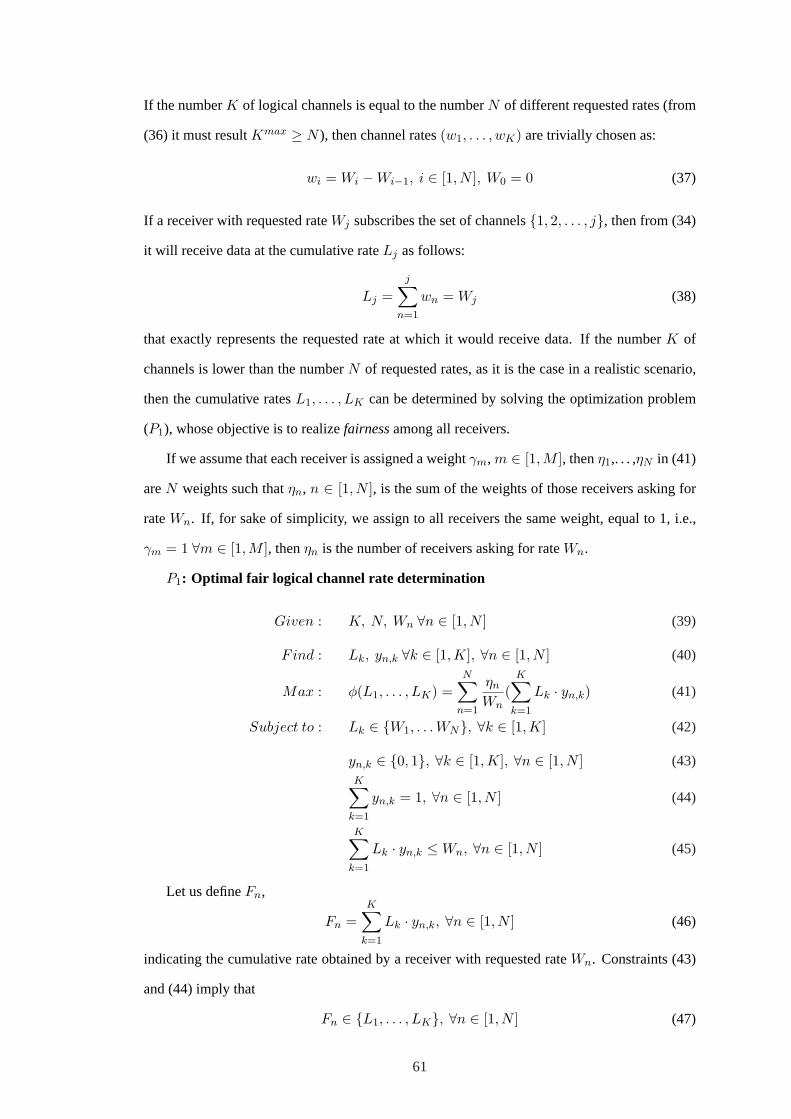
If the numberK of logical channels is equal to the numberN of different requested rates (from
(36) it must resultKmax ≥ N ), then channel rates(w1, . . . , wK) are trivially chosen as:
wi = Wi −Wi−1, i ∈ [1, N ], W0 = 0 (37)
If a receiver with requested rateWj subscribes the set of channels1, 2, . . . , j, then from (34)
it will receive data at the cumulative rateLj as follows:
Lj =j∑
n=1
wn = Wj (38)
that exactly represents the requested rate at which it would receive data. If the numberK of
channels is lower than the numberN of requested rates, as it is the case in a realistic scenario,
then the cumulative ratesL1, . . . , LK can be determined by solving the optimization problem
(P1), whose objective is to realizefairnessamong all receivers.
If we assume that each receiver is assigned a weightγm, m ∈ [1, M ], thenη1,. . . ,ηN in (41)
areN weights such thatηn, n ∈ [1, N ], is the sum of the weights of those receivers asking for
rateWn. If, for sake of simplicity, we assign to all receivers the same weight, equal to 1, i.e.,
γm = 1 ∀m ∈ [1,M ], thenηn is the number of receivers asking for rateWn.
P1: Optimal fair logical channel rate determination
Given : K, N, Wn ∀n ∈ [1, N ] (39)
Find : Lk, yn,k ∀k ∈ [1,K], ∀n ∈ [1, N ] (40)
Max : φ(L1, . . . , LK) =N∑
n=1
ηn
Wn(
K∑
k=1
Lk · yn,k) (41)
Subject to : Lk ∈ W1, . . . WN, ∀k ∈ [1,K] (42)
yn,k ∈ 0, 1, ∀k ∈ [1,K], ∀n ∈ [1, N ] (43)K∑
k=1
yn,k = 1, ∀n ∈ [1, N ] (44)
K∑
k=1
Lk · yn,k ≤ Wn, ∀n ∈ [1, N ] (45)
Let us defineFn,
Fn =K∑
k=1
Lk · yn,k, ∀n ∈ [1, N ] (46)
indicating the cumulative rate obtained by a receiver with requested rateWn. Constraints (43)
and (44) imply that
Fn ∈ L1, . . . , LK, ∀n ∈ [1, N ] (47)
61

Once the cumulative ratesFn are determined by solving the problem (P1), then the correspond-
ing channels rates are easily computed as follows:
wj = Lj − Lj−1, j ∈ [1,K], L0 = 0 (48)
Now we present an original algorithm to exactly solve the problem (P1) in polynomial time.
An example of the algorithm in a simplified scenario will be given after its formal description
(Fig. 19-23). The algorithm goes through two stages:
1. We build a directed graphG(V, E), where nodes of the graph are theN different requested
rates together with an exit nodenexit, i.e., V = W1, . . . , WN ∪ nexit, thus |V | =
N + 1,
2. We solve a maximum cost path problem from nodeW1 to nodenexit in the constructed
graphG(V, E). At this point, all the nodes belonging to this path will be those cumulative
channel ratesL1, . . . , LK that form an optimal solution of problem (P1).
Let us now assumeL1 = minL1, · · · , LK = W1. If L1 > W1, sinceLK > . . . > L1 > W1
from (48), then receivers that asked for rateW1 could not subscribe any channel without incur-
ring in data loss. In fact, if they subscribed channelw1 = L1 > W1, they would be overwhelmed
by arriving packets. Thus, this means that it must necessarily beL1 = W1, as initially assumed.
The proposed algorithm to exactly solveP1, proceeds into steps, hereafter described:
• Step 1:
Starting from node (rate)W1, a link (1, j) from W1 to Wj (∀j = 2, · · · ,K + 1) is
added to the graph. Since there areK channels, the set of all possible values forL2 is
W2, . . . , WK+1, thus at leastK − 2 valuesWK+2, . . . , WN remain for the others
K − 2 cumulative ratesL3, . . . , LK .
The costc(1, j) of each link(1, j) (∀j = 2, · · · ,K+1) is the partial value of the objective
function (41) determined by the choiceL1 = W1 for all those receivers that ask for rates
from W1 to Wj−1. Thus, the cost of link(1, j) is defined as:
c(1, j) =j−1∑
n=1
ηn · W1
Wn(49)
• Step i, i=2,. . . ,K-1:
62

A link (i, j) from Wi to Wj (∀j = i + 1, · · · ,K + i) is added to the graph. The set
Wi+1, . . . , WK+i is determined by considering that at this step, values of the cumu-
lative rates,L1 = W1, . . . , Li = Wi, could have already been assigned (it is only an ad-
missible solution, not necessarily the optimal one). In this limit case, at leastK-i-1 val-
uesWK+i+1, . . . , WN must remain for the othersK-i-1 values of the cumulative rate
Li+2, . . . , LK .
The costc(i, j) of the link (i, j) is defined as:
c(i, j) =j−1∑
n=i
ηn · Wi
Wn(50)
The costc(i, j) is the partial value of the objective function (41) determined by the choice
of the cumulative rateWi for all those receivers that ask for rates fromWi to Wj−1.
• Step i, i = K, . . . , N − 1:
A link (i, j) from Wi to Wj (∀j = i+1, · · · , N ) is added to the graph. The costc(i, j) of
link (i, j) is defined according to (50). Furthermore, a link from node (rate)Wi to the exit
nodenexit is added to the graph. In fact atStep i, i = K, all K values of the cumulative
ratesL1, . . . , LK could have already been assigned. If there are no more cumulative rates,
i.e., no more channels, then the cumulative rateLK = Wi is assigned to all the receivers
that ask for rates fromWi to WN .
The costc(i, nexit) of the link (i, nexit) is defined as:
c(i, nexit) =N∑
n=i
ηn · Wi
Wn(51)
Eq. (51) represents the partial value of the objective function determined by the choice of
the cumulative rateWi for all the receivers that ask for rates formWi to WN .
• Step N:
Finally, only one link(N, nexit) from node (rate)WN to the exit nodenexit is added to
the graph. Costc(N, nexit) of the link (N,nexit) is simply c(N,nexit) = ηN , which is
the contribution to the objective function of the choiceLK = WN .
Example. Let us considerN = 5 different requested ratesW1 < W2 < . . . < W5 and let
us suppose that onlyK = 3 channels are available. Let us suppose, for sake of clearness, that
ηn = 1, n = 1, . . . , 5.
63

Figure 19: Determining channel rates:Step 1
Figure 20: Determining channel rates:Step 2
Figure 21: Determining channel rates:Step 3
64

Figure 22: Determining channel rates:Step 4
• Step 1:
L1 is set toW1 and links from nodeW1 to nodesW2, W3 andW4 are added to the graph
(Fig. 19). There is no link fromW1 to W5 because the possible cumulative rates are three
(K = 3) and it cannot beL2 = W5. As exposed before, the cost of each link(W1,Wj) is
the contribution of the choiceL2 = Wj to the objective function (41).
• Step 2:
Links from nodeW2 to nodesW3, W4 andW5 are added to the graph (Fig. 20). The cost
of each link(W2,Wj) is the contribution of the choiceL3 = Wj to (41).
• Step 3:
Links from nodeW3 to nodesW4, W5 andnexit, are added to the graph (Fig. 21). The
cost of each link(W3,Wj) is the contribution of the choiceL3 = Wj to the objective
function (41) whenL2 = W3, while the cost of the link(W3, nexit) is the contribution of
the choiceL3 = W3 to the objective function (41) whenL2 = W2.
• Step 4:
Links from nodeW4 to nodesW5 and from nodeW4 to nexit are added to the graph (Fig.
22). The cost of link(W4,W5) is the contribution of the choiceL3 = W5 to the objective
function (41) whenL2 = W4, while the cost of the link(W4, nexit) is the contribution of
the choiceL3 = W4 to (41) whenL2 = W2 or L2 = W3.
• Step 5:
65
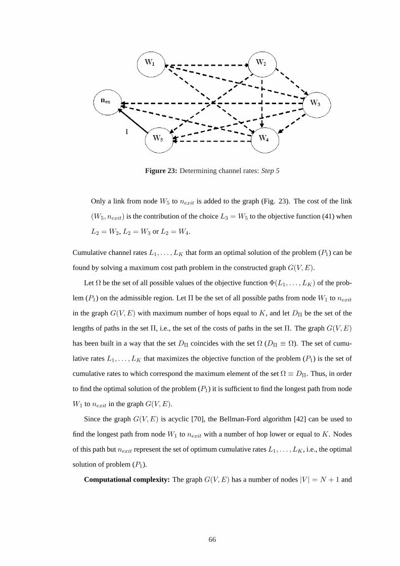
Figure 23: Determining channel rates:Step 5
Only a link from nodeW5 to nexit is added to the graph (Fig. 23). The cost of the link
(W5, nexit) is the contribution of the choiceL3 = W5 to the objective function (41) when
L2 = W2, L2 = W3 or L2 = W4.
Cumulative channel ratesL1, . . . , LK that form an optimal solution of the problem (P1) can be
found by solving a maximum cost path problem in the constructed graphG(V, E).
Let Ω be the set of all possible values of the objective functionΦ(L1, . . . , LK) of the prob-
lem (P1) on the admissible region. LetΠ be the set of all possible paths from nodeW1 to nexit
in the graphG(V, E) with maximum number of hops equal toK, and letDΠ be the set of the
lengths of paths in the setΠ, i.e., the set of the costs of paths in the setΠ. The graphG(V,E)
has been built in a way that the setDΠ coincides with the setΩ (DΠ ≡ Ω). The set of cumu-
lative ratesL1, . . . , LK that maximizes the objective function of the problem (P1) is the set of
cumulative rates to which correspond the maximum element of the setΩ ≡ DΠ. Thus, in order
to find the optimal solution of the problem (P1) it is sufficient to find the longest path from node
W1 to nexit in the graphG(V, E).
Since the graphG(V,E) is acyclic [70], the Bellman-Ford algorithm [42] can be used to
find the longest path from nodeW1 to nexit with a number of hop lower or equal toK. Nodes
of this path butnexit represent the set of optimum cumulative ratesL1, . . . , LK , i.e., the optimal
solution of problem (P1).
Computational complexity: The graphG(V, E) has a number of nodes|V | = N + 1 and
66

a number of links equal to
|E| = (K − 1) · (N −K − 1) +N∑
i=k
(1 + N − i) (52)
The Bellman-Ford algorithm, which dominates most of the computing time of the algorithm,
has a computational complexityO(|V | · |E|). Thus, the complexity of the proposed algorithm
for the channel rate determination isO(K ·N2).
3.2.2 Least cost source rooted trees
The classical optimization problem in multicast routing is theSteiner tree problem in networks
(SPN) [9]. If a network can be modelled by a directed graphG(V, E) consisting of a set of
nodesV and a set of arcsE, each node of the graph represents a router of the network and
each arc of the graph represents a link of the network. LetT = r1, r2, . . . , rm ∈ V be a
group of nodes inG ands ∈ V , s /∈ T , theSteiner tree problemis to find the least-cost tree
connecting the sources with the group of destinationsT with the minimum total cost over all
links. If each destinationrk ∈ T has a bandwidth requirement ofWk units on each edge of the
path froms to rk, then theBandwidth-Constrained Least-Cost Steiner tree problemhas to be
solved. This problem is to find theleast-costtree that respects the bandwidth requirementsWk
on each path from the sources to the receiverrk. Since both theSteiner tree problemand the
Bandwidth-Constrained Least-Cost Steiner tree problemare NP-complete, efficient algorithms
to solve these problems in polynomial time attain only approximate solution [147][9].
3.2.3 DIMRO in non-QoS-aware networks
By simply minimizing the cost of multicast trees without taking into account the link bandwidth
availability, bottlenecks might occur in the network. In fact, since many multicast trees may use
the same set of links, these links could be overloaded while other links in the network remain
under-utilized.
The DIMRO algorithm proposed in this work follows a different approach to tackle the
problem of bandwidth bottlenecks, one of the main reasons for low network performance. The
multicast source rooted tree is built by choosing those paths that result least loaded to obtain
a smooth load balancing. DIMRO obtains an optimal distribution of network resources which
leads to maximize as much as possible the number of multicast trees that can be set up in the
network.
67

Let us consider a multirate multicast scenario where receivers ask for different rates. If
K channels with ratew1, . . . , wK are used in the layering scheme, thenK cumulative rate
L1, . . . , LK are available. Lets be the source node, and let us suppose that the multicast group
is made up ofM receivers. The DIMRO algorithm proceeds as it follows.
• Step 0:
Receivers are ordered from the highest rate to the lowest one. At the end of this step
we have an ordered set ofM receiversr1, . . . , rM, with requested cumulative rates
F1 ≥ F2 ≥ . . . ≥ FM (Fj ∈ L1, . . . , LK, j = 1, . . . , M ). Receivers fromr1 to rM are
connected to the source node progressively. In this way, receiverri can reuse resources
already exploited on paths from the source to receiversr1, . . . , ri−1. These receivers, in
fact, ask for ratesF1 ≥ F2 ≥ . . . ≥ Fi−1 ≥ Fi.
Let Spath(s, rk) be the set of all feasible paths froms to rk. A pathp(s, rk) from sources
to receiverrk is feasible ifbuv ≥ Fk for all its links, wherebuv is the available bandwidth
in link (u, v).
• Step k, k = 1, . . . , M :
The algorithm chooses the pathp(s, rk) ∈ Spath(s, rk) that minimizes the following
function:
fp(s, rk) =∑
(u,v)∈p(s,rk)
auv
(1− ρuv)α,
p(s, rk) ∈ Spath(s, rk) (53)
1. ρuv is the link(u, v) utilization and it is defined as:
ρuv =Buv − (buv − Fk)
Buv=
Buv − βuv
Buv(54)
whereBuv is the total bandwidth capacity of link(u, v), Fk is the bandwidth ex-
ploited on link(u, v) by receiverrk andβuv = buv − Fk is the residual bandwidth
of link (u, v). It is worth pointing out thatρuv is calculated after thatbuv has been
decremented byFk.
2. The exponentα = α(|V |, |E|, F , B) in (53) is a function of the number of nodes
|V | and links|E|, the average rateF requested by receivers, and the average net-
work link bandwidthB. According to accurate empirical observations (described
68
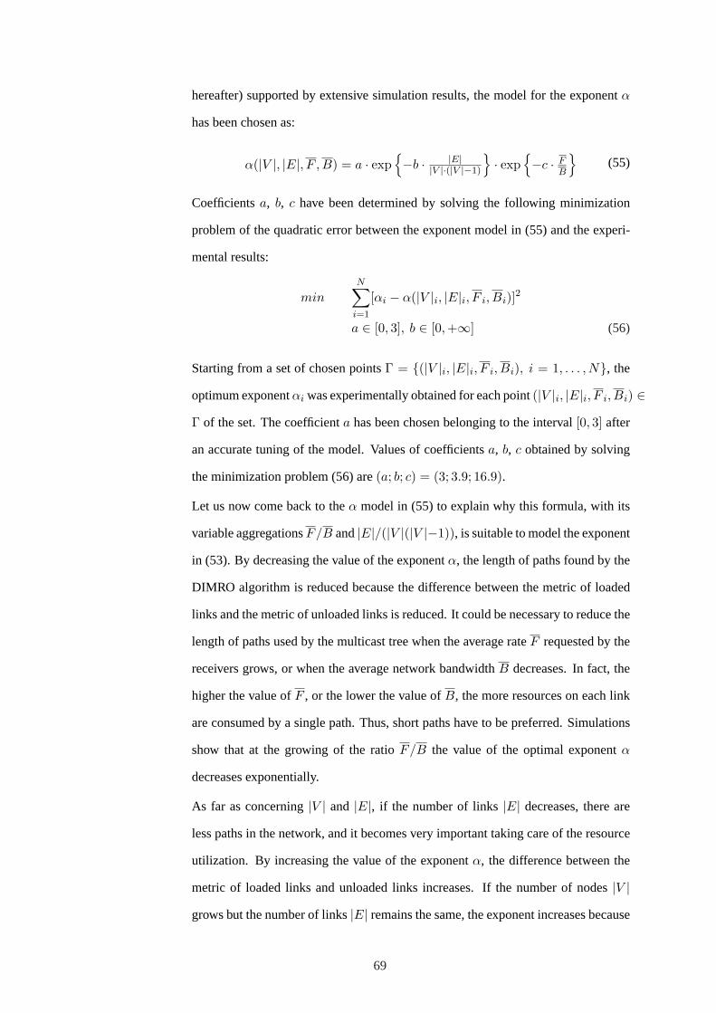
hereafter) supported by extensive simulation results, the model for the exponentα
has been chosen as:
α(|V |, |E|, F , B) = a · exp−b · |E|
|V |·(|V |−1)
· exp
−c · F
B
(55)
Coefficientsa, b, c have been determined by solving the following minimization
problem of the quadratic error between the exponent model in (55) and the experi-
mental results:
min
N∑
i=1
[αi − α(|V |i, |E|i, F i, Bi)]2
a ∈ [0, 3], b ∈ [0, +∞] (56)
Starting from a set of chosen pointsΓ = (|V |i, |E|i, F i, Bi), i = 1, . . . , N, the
optimum exponentαi was experimentally obtained for each point(|V |i, |E|i, F i, Bi) ∈Γ of the set. The coefficienta has been chosen belonging to the interval[0, 3] after
an accurate tuning of the model. Values of coefficientsa, b, c obtained by solving
the minimization problem (56) are(a; b; c) = (3; 3.9; 16.9).
Let us now come back to theα model in (55) to explain why this formula, with its
variable aggregationsF/B and|E|/(|V |(|V |−1)), is suitable to model the exponent
in (53). By decreasing the value of the exponentα, the length of paths found by the
DIMRO algorithm is reduced because the difference between the metric of loaded
links and the metric of unloaded links is reduced. It could be necessary to reduce the
length of paths used by the multicast tree when the average rateF requested by the
receivers grows, or when the average network bandwidthB decreases. In fact, the
higher the value ofF , or the lower the value ofB, the more resources on each link
are consumed by a single path. Thus, short paths have to be preferred. Simulations
show that at the growing of the ratioF/B the value of the optimal exponentα
decreases exponentially.
As far as concerning|V | and |E|, if the number of links|E| decreases, there are
less paths in the network, and it becomes very important taking care of the resource
utilization. By increasing the value of the exponentα, the difference between the
metric of loaded links and unloaded links increases. If the number of nodes|V |grows but the number of links|E| remains the same, the exponent increases because
69

the number of paths decreases. Simulations show that at the decreasing of the ratio
|E|/(|V |(|V | − 1)) the value of the optimal exponentα grows exponentially.
3. The binary variableauv is equal to zero if link(u, v) already belongs to the tree,
otherwise it is 1. If the setSpath(s, rk) is not empty, letp(s, rk) be the path from
the sources to the receiverrk that minimizes the function in (53). On each link
(u, v) belonging top(s, rk), if auv = 0, the value of the available bandwidth is not
updated and uses those bandwidth resources already exploited by a pathp(s, rj),
with Fj ≥ Fk. Conversely, ifauv 6= 0, then new resources must be consumed and
the new value of the available bandwidth isb′uv = buv−Fk. Then the binary variable
auv is set to zero in order not to consider the cost of link(u, v) for those future paths
which will exploit it.
Let us point out that atStep k, k = 1, . . . ,M , the optimal pathp(s, rk) ∈ Spath(s, rk) can
be found using a shortest path algorithm (as Dijkstra or Bellman-Ford algorithm), where the
length of each link in the network is set to:
duv =
auv(1−ρuv)α if buv ≥ Fk
∞ if buv < Fk or (u, v) /∈ E(57)
In this work we use the Bellman-Ford algorithm which finds a spanning tree of the shortest
paths from the source to all other nodes of the graph. The pathp(s, n) from nodes to noden,
solution of (53), is the one that minimizes the function:
∑
(u,v)∈p(s,n)duv (58)
Computational complexity: If the number of receivers isM , the DIMRO algorithm builds
the multicast tree by computing for as many asM times the spanning tree (Bellman-Ford al-
gorithm). Since the time complexity of the Bellman-Ford algorithm isO(|V | · |E|), then the
computational complexity of the algorithm isO(M · |V | · |E|).
3.2.4 DIMRO in DiffServ aware networks
In this section the DIMRO algorithm is integrated into a DiffServ network. Let us consider a
multirate multicast scenario where receivers ask for the same data content but different rates
and different qualities of service (QoS), mapped into the respective service class according to
70

[34][35]. In particular, DIMRO can build source rooted tree for real time multicast communi-
cation, by adopting the Expedited Forwarding (EF) DiffServ service class [90], and for non real
time communication, by adopting the Assured Forwarding (AS) DiffServ service class [81].
The DIMRO algorithm, integrated in a DiffServ network, allows a receiver to reuse the
bandwidth already exploited by receivers asking for higher service classes without any extra
cost for the network. By building a path from the sources to a receiverr, the DIMRO algorithm
can reuse some sub-paths already exploited by higher service class receivers. Thus, receiver
r obtains abetterQoS, and the network saves resources because bandwidth already exploited
by other receivers is reused for receiverr. DIMRO in a DiffServ network proceeds into steps,
described hereafter.
• Step 0:
Receivers are ordered according to their service class and rate. Let us consider a setR
made up ofM receivers. LetCL = cl1, . . . , clL be the set of service classes requested
by receivers, wherecl1 is the highest service class andclL is the lowest one.CL is a
subset of all service classes supported by the DiffServ architecture [34][35]. The set of
receiversR is partitioned intoL = |CL| subsets:
R =L⋃
i=1
Ri (59)
SubsetRi is made up of those receivers asking for service classcli, i = 1, . . . , L. Re-
ceivers in each subsetRi, are ordered from the highest rate to the lowest one. Let us
consider a partitioned and ordered setR made up ofM receivers. Letrik be the receiver
k in the subsetRi with requested rateF ik. |Ri| stands for the cardinality ofRi, andi
represents the associated service class.
• Step j, j = 1, . . . , L:
DIMRO connects the sources with all those receivers asking for service classcli. Initially,
the binary variablesauv are set to 1 for each network link(u, v). For receiverrik, k =
1, . . . , |Ri|, auv are set to 0 for all those links(u, v) already used by receivers that ask for
higher service class and higher or equal rate thenrik. In fact, resources already exploited
by the tree on these links could be used byrik without any added cost.
71

Let buv(cli) be the available bandwidth of link(u, v) for the service classcli. A pathp(s, rik)
from sources to a receiverrik asking for cumulative rateF i
k is feasible ifbuv(cli) ≥ F ik for all
its links. DIMRO algorithm chooses that feasible pathp(s, rik) from s to ri
k that minimizes the
function:
fp(s, rik) =
∑
(u,v)∈p(s,rik)
auv
(1− ρuv(cli))α,
p(s, rik) ∈ Spath(s, ri
k) (60)
whereSpath(s, rik) is the set of feasible paths froms to ri
k.
Exponentα is defined as in (55), and utilizationρuv(cli) of the link (u, v) is calculated as
follows:
ρuv =Buv(cli)− [buv(cli)− F i
k]Buv(cli)
(61)
whereBuv(cli) is the bandwidth capacity of link(u, v) for the classcli andF ik is the cumulative
rate requested byrik.
For each link(u, v) belonging to pathp(s, rik), if auv = 0 then the available bandwidth
buv(cli) is not updated and the new path uses those resources already exploited by other re-
ceivers. On the contrary, ifauv 6= 0, then new resources have to be exploited and the new value
of the available bandwidth becomesb′uv(cli) = buv(cli) − F i
k. Then the binary variableauv is
set to zero.
The DIMRO algorithm determines the pathp(s, rik) by using a modified shortest-path al-
gorithm. Common shortest path algorithms could choose one of those possible paths with zero
cost froms to n, but p(s, rik) might not be correct. To determine a correct path the algorithm
proceeds as it follows.
Starting from nodes, the first link (u, v) belonging top(s, rik) with auv 6= 0 is found.
Among all those paths in the tree exploiting a bandwidth equal or greater thanF ik and passing
through nodeu, it is chosen the one which uses the highest service class. Let us indicate this
path withpu. The new pathp(s, rik) from s to ri
k is the concatenation of the sub-path froms to
nodeu, belonging to pathpu, and the sub-path from nodeu to rik, belonging top(s, ri
k).
Example. Figure 24 shows a multicast tree where receiverr1 (node 6) asks for a rateF1 = 2
and a QoS mapped into service class A, receiverr2 (node 8) asks for a rateF2 = 3 and a QoS
mapped into service class B, and receiverr3 (node 7) asks for a rateF3 = 2 and a QoS mapped
into service class C. Path from sources, node 1, to receiverr1 is the first to be built. Receiver
72

Figure 24: Correct path computation
r2 asks for a service class B but a rateF2 = 3 > F1 = 2, thus the binary variablesauv are
not set to 0 on links of path from node 1 to node 6. Path from node 1 to node 8 is built. Let
p(s, ri) be the path from sources to receiverri. Receiverr3 asks for a service class C and a
rateF3 = F1 = 2 < F2 = 3 thus, on each link of pathsp(s, r1) andp(s, r2), auv are set
to 0 becauser3 can reuse resources already exploited by other receivers. By using a common
shortest path algorithm, pathp = 1 → 2 → 3 → 5 → 7 might be found from sources to
receiverr3 (node 7) because paths1 → 2 → 3 → 5 and1 → 4 → 3 → 5 have both cost
equal to zero. The point is that this pathp cannot be taken into consideration since link(3, 5)
belongs only to the path1 → 4 → 3 → 5 → 8) (p(s, r2) in Fig. 24) and not to the path
1 → 2 → 3 → 6 (p(s, r1) in Fig. 24). For the mentioned reason, it should be clear that
the correct path is1 → 4 → 3 → 5 → 7. Once the shortest path algorithm has determined
a path from the sources, node 1, to receiverr3, node 7, the last node of the zero cost path is
determined, in Fig. 24 node 5. All paths connecting the source with those receivers that ask for
a higher or equal service class and a higher or equal requested rate thanr3 are visited (in Fig. 24
path froms to r1 and froms to r2). Only path froms to r2 has a sub-path1 → 4 → 3 → 5from s to node 5. Thus, path1 → 4 → 3 → 5 is chosen among all path with zero cost from
s to node 5. Finally, the correct paths1 → 4 → 3 → 5 → 7 from s to r3 is selected.
73

3.3 DIMRO-GS - DiffServ-Integrated Multicast algorithm for Inter-net Resource Optimization Group Shared applications
In this section, we present DIMRO-GS, a novel algorithm to efficiently build shared trees for
group shared multicast communications. A shared tree is a generalization of a source rooted
tree. In a source rooted tree the source node multicasts data to a set of receiver nodes, whereas
in a shared tree each member node can multicast data to all the other member nodes (videocon-
ference is probably the most common multicast application requiring a shared tree, but many
others applications are conceivable such as distributed games, file sharing, collaborative group-
ware, replicated database, etc.).
In Section 3.3.1 we explain how DIMRO-GS works in non-QoS-aware networks and show
how this algorithm manages to keep low the probability of bottleneck occurrence. In Section
3.3.2 we point out the main improvements in DIMRO-GS when a QoS-aware network is consid-
ered. In this last case the full set of features, which DIMRO-GS is endowed with, is described
and analyzed.
As briefly introduced in Section 3.1, a possible approach to build a shared tree is proposed
in the Core Based Protocol (CBT) [21][22] and in its enhanced version (CBTv2) [20]. The CBT
protocol connects each member node to acore nodeusing bi-directional shortest paths. The
main drawback with this approach is the traffic concentration occurring in the core node. In
fact, all data sent to a member node from all the other member nodes pass through the same
path from the core node to the destination member node. Thus, some link might be overloaded,
specially in multicast applications with high bandwidth requirements. Moreover, multicast trees
set up with this approach are quite easy to be computed, but are far from being optimized. Let
us consider an extreme example to catch the inefficiency of this protocol: if two member nodes
had a link connecting each other, still their traffic would pass through the core node, no matter
the state of their common link.
To avoid traffic concentration a shared tree can be computed by separately findingM source
rooted trees (whereM is the number of member nodes). The source rooted treei, i = 1, . . . ,M
has the member nodeni as root and all the other member nodesnj , j = 1, . . . , M (with j 6= i),
belonging to the tree, not necessarily as leaves. The FTM (Feasible solutions using adapted TM
algorithm) algorithm, proposed in [151][107], follows this approach. The source rooted treei,
i = 1, . . . , M connects the root nodeni with the member nodenj , j = 1, . . . , M , j 6= i, by
74

using the path with the greatest capacity from nodeni to nodenj . The bottleneck of a path is
characterized as the used link with the minimum available bandwidth, and the path bandwidth
capacity is defined as the available bandwidth of its bottleneck. The path with the greatest
bandwidth capacity from nodeni to nodenj is called thewidest path. The FTM algorithm uses
information obtained by the Breadth First Search procedure (BFS) [65]. For each member node
the BFS procedure builds a tree rooted at the member node and connecting each network node
with this member node by exploiting thewidest path paradigm criterion. After M BFS trees
are built rooted at each group memberni, the detailed pieces of information about thewidest
pathconnecting each pair of member nodes are available.
In the next step, the FTM procedure buildsM multicast source rooted trees, one for each
group memberni. As far as concerning the member nodeni, paths with the maximum band-
width capacity will be used by the source nodeni to join all the other group member. If two
or more paths with the same bandwidth capacity are found at the same time, the one with the
least cost is selected. In order to generate each multicast tree, two tables must be available: the
bandwidth capacitytable and thepath costtable. These tables are bothM · |V | in size, where
M is the number of members and|V | is the number of network nodes.
Computational complexity: The FTM computational complexity is dominated by the BFS
complexity which isO((|V |+ |E|) · |V |2). Thus, buildingM multicast trees by exploiting the
FTM algorithm, isO(M · (|V |+ |E|) · |V |2).
3.3.1 DIMRO-GS in non-QoS aware networks
In Section 3.2 the DIMRO algorithm has been presented. This algorithm can be extended to
the multicast shared tree case. We called this extended algorithm DIMRO-GS (Group Shared
DIMRO). If there areM group members, the shared tree can be set up by buildingM source
rooted trees, each one having a different group member as root and all the other group members
belonging to the tree, not necessarily as leaves. Each source rooted tree can be built according
to the DIMRO algorithm [124]. Let us assume that each group member has the same band-
width requirement, i.e.,Wk = W , k = 1, . . . , M . In this case, the first step of the DIMRO
algorithm, aimed at ordering receivers according to their bandwidth requirement, is skipped.
WhenM source rooted trees are computed, the shared tree is completed. From then onwards,
each member group can send data to all the other members and receive data from all the other
75

members.
Computational complexity: In the shared tree case, ifM is the number of group members,
thenM source rooted trees have to be built. The computational complexity for each source
rooted tree by using the DIMRO algorithm isO(M · |V | · |E|), as seen in Section 3.2.3; thus,
the computational complexity of the DIMRO-GS algorithm becomesO(M2 · |V | · |E|).It has been exposed in the previous subsection that the computational complexity of FTM
algorithm isO(M · (|V |+ |E|) · |V |2). Since in most practical caseM << |V |, the computa-
tional complexity of the proposed algorithm is lower than the FTM complexity. Furthermore,
FTM needs twoM · |V | tables that must be stored in memory, while in DIMRO-GS no tables
are required.
3.3.2 DIMRO-GS in DiffServ aware networks
In this section the DIMRO-GS algorithm is integrated into a DiffServ aware network. Let us
consider a multicast scenario where group members in a group shared communications can
ask for a different quality of service (QoS). The QoS requirements of each group member are
mapped into the associated service class. In particular, DIMRO-GS can build group shared tree
for both real time multicast communications, by adopting the Expedited Forwarding (EF) Diff-
Serv service class [90], and non real time communications, by adopting the Assured Forward-
ing (AS) DiffServ service class [81]. The DIMRO-GS algorithm integrated in a DiffServ aware
network allows a group member acting as receiver to reuse the bandwidth already exploited
by group members asking for higher service classes, without any extra cost for the network.
By building a path from a group members, acting as source, to a group memberr, acting as
receiver, the DIMRO-GS algorithm can reuse some sub-paths already exploited by group mem-
bers, acting as receivers, with more stringent QoS requirements. Thus, group memberr obtains
a betterQoS and the network saves resources because bandwidth already exploited by other
group members is reused for group memberr. The DIMRO-GS algorithm in a DiffServ aware
network proceeds as it follows.
Let us consider a setR made up ofM group members. At the first step, group members are
ordered from the highest service class to the lowest one. The setR is ordered per service class,
thus, ifk < h, then member groupnk asks for a higher or equal service class thennh.
Example. Let us consider a simple DiffServ architecture with only four different classes of
76

service:A, B, C, D. SupposeA is the highest service class whereasD is the lowest one. Let
us indicate a group memberr with the couple(F ; C) = (RequestedRate; ServiceClass) rep-
resenting the rate and service class requested by group memberr. Let us consider the following
multicast group:R = (1;B), (1;A), (1;B), (1; D), (1;C), (1; C). The algorithm proceeds
as it follows:
• Step 0:
The multicast group is sorted per service class in a lexicographic order, as shown here-
after:
R∗ = (1;A), (1;B), (1;B), (1; C), (1;C), (1;D).
• Step i, i = 1, . . . , M :
DIMRO-GS uses the DIMRO algorithm to builds a source rooted tree with the member
nodeni as root and all the other member nodes belonging to the tree. At the beginning
of Step i, the binary variablesauv are initialized to 1 for each network link(u, v). Let clj
be the service class requested by the group membernj , j = 1, . . . ,M , nj 6= ni, acting
as receiver, and letbuv(clj) be the available bandwidth for the service classclj on link
(u, v). A pathp(ni, nj) from the nodeni to a nodenj is feasible ifbuv(clj) ≥ W for all
its links (W is the rate requested by each group member). For each group membernj ,
j = 1, . . . , M , nj 6= ni the DIMRO algorithm chooses that feasible pathp(ni, nj) from
the nodeni to a nodenj that minimizes the function:
fp(ni, nj) =∑
(u,v)∈p(ni,nj)
auv
(1− ρuv(clj))α,
p(ni, nj) ∈ Spath(ni, nj) (62)
whereSpath(ni, nj) is the set of all feasible paths from the nodeni to a nodenj . For each
link (u, v) belonging to pathp(ni, nj), if auv = 0, then the available bandwidthbuv(clj) is
not updated, and the new path uses those resources already exploited by another member
group, acting as receiver, that asks for a higher or equal service class. On the contrary, if
auv 6= 0, then new resources must be exploited and, thus, the new value of the available
bandwidth becomesb′uv(clj) = buv(clj)−W . Then the variableauv is set to 0. This way
the path from the nodeni to a nodenk, k = j + 1, . . . , M , can reuse resources already
used on pathp(ni, nj) without any adding cost for the network.
77

Table 10: Network parameters
α β B nodesNetwork 1 0.2 0.4 100 Mbps 100Network 2 0.3 0.6 100 Mbps 100
3.4 Simulation Results
3.4.1 Random network model
To ensure a fair evaluation of different routing algorithms, a random network has been gen-
erated according to the Waxman’s model [152][40]. In the Waxman’s model, network nodes
are randomly distributed across a Cartesian coordinate grid. Links are added to the graph by
considering all possible pairs(u, v) of nodes and by using the probability function:
Pe(u, v) = β · exp(− duv
α · L)
(63)
wherePe(u, v) is the existence probability of a link between nodesu andv, duv is the Euclidean
distance between the nodeu and the nodev, L is the maximum possible distance between a pair
of nodes,α andβ are parameters belonging to the range (0,1]. A highα value increases the
number of connections to nodes further away, while a highβ value increases the node degree.
Unlike the original Waxman’s model [152], we suppose that each link added to the network
is bi-directional. The bandwidth capacityBuv of each link(u, v) is randomly generated using an
uniform distribution with mean bandwidthB. Consequently, the link(u, v) bandwidth capacity
Buv may be different from the link(v, u) bandwidth capacityBvu.
In this work, two different one hundred node random networks are generated, according to
Tab. 10. Network 2 has a higher number of links than Network 1, according to the probability
function (63). The average bandwidth in both networks isB = 100 Mbps.
3.4.2 DIMRO Performance Evaluation
The DIMRO algorithm is compared to the optimal solution of the Steiner tree problem when all
link costs are equal to 1. If every links have a cost equal to 1, then theminimum-weight treethat
spans all group members is the multicast tree that uses the least number of links.
The minimum-weight tree is found by solving the flow formulation of the Steiner tree prob-
lem proposed in [44][154]. We implemented the Integer Linear Programming (ILP) problem in
AMPL [64] and solved it with the CPLEX [2] solver.
78

The DIMRO algorithm and the optimal solution of the Steiner tree problem with unitary
costs are compared by using two metrics: theRejection Rateand theNetwork Load. For each
simulation campaign several experiments have been run to ensure a 95% relative confidence
intervals smaller than 5%.
Starting from a completely unloaded Waxman network [152], it is requested to build a fixed
number of source rooted trees, in the following theNumber of Requested Trees. Multicast
groups are sequentially randomly generated. Multicast group members (source and receivers)
are randomly chosen among network nodes. The number of receivers for each multicast group
is uniformly distributed from 5 to 15, and the bandwidth request of each receiver is uniformly
distributed from0.1 to 2 Mbps.
To evaluate the performance of the DIMRO algorithm in the different simulated scenarios,
we use two metrics, theRejection Rateand theNetwork Load.
1. TheRejection Rateis defined as:
Rejection Rate=Number of Rejected Trees
Number of Requested Trees(64)
where theNumber of Requested Treesis the total number of source rooted trees sequen-
tially generated, while theNumber of Rejected Treesis the number of requested source
rooted trees that cannot be built because there are not enough resources in the network.
2. TheNetwork Loadρ is defined as:
ρ =
∑(u,v)∈E ρuv
|E| (65)
whereE is the set of network links,|E| its cardinality, andρuv is theLink Loadof link
(u, v), defined as:
ρuv =Used Bandwidth of link (u,v)
Bandwidth Capacity of link (u,v)(66)
Figure 25 shows that the DIMRORejection Ratein Network 1 is lower than theRejection
Rateof the Optimal solution of the Steiner Tree Problem (OSTP) withcuv = 1. TheRejection
Rateis approximately the same until theNumber of Requested Treesis less than 2500. When
the Number of Requested Treesovercomes this threshold, the DIMRO algorithm has a lower
Rejection Rate.
Both DIMRO and OSTPRejection Ratesgrow at the growing of theNumber of Requested
Treesbecause the same bottlenecks occur. These bottlenecks depend on the network topology
79

1500 2000 2500 3000 3500 4000 4500 5000 5500 60000
5
10
15
20
25
30
35
40DIMRO and OSTP Rejection Rate in Network 1
Number of Requested Trees
Rej
ectio
n R
ate
[%]
DIMROOSTP
Figure 25: DIMRO and OSTPRejection Ratein Network 1
1500 2000 2500 3000 3500 4000 4500 5000 5500 600020
30
40
50
60
70
80DIMRO and OSTP Network Load in Network 1
Number of Requested Trees
Net
wor
k Lo
ad [%
]
DIMROOSTP
Figure 26: DIMRO and OSTPNetwork Loadin Network 1
80

0.7 0.8 0.9 1 1.1 1.2 1.3 1.4 1.5 1.6 1.7 1.8
x 104
0
5
10
15
20
25
30
35DIMRO and OSTP Rejection Rate in Network 2
Number of Requested Trees
Rej
ectio
n R
ate
[%]
DIMROOSTP
Figure 27: DIMRO and OSTPRejection Ratein Network 2
and cannot be avoided, but the DIMRORejection Rateis lower because bottlenecks occur later.
Figure 26 shows that the DIMRONetwork Loadis lightly lower than the OSTPNetwork Load
until theRejection Rateis the same. Then, since DIMRO rejects less trees, itsNetwork Loadis
higher than the OSTP one.
Network 2 has a higher number of links than Network 1, according to (63) and the network
parameters in Tab. 10. In this second type of network, the DIMRORejection Rateis significantly
lower than the OSTPRejection Rate(Fig. 27). This is because lessunavoidablebottlenecks
exist. Anunavoidablebottleneck is a bottleneck that depends on the network topology and not
on the algorithm used in the network. For example, if only one path exists between two nodes,
all communications between these two nodes must use this path. Since Network 2 has a higher
number of links, the number of possible paths between two nodes grows, and it is easier for the
DIMRO algorithm to avoid bottlenecks. A lowerNetwork Load(Fig. 26 and Fig. 28) with a
higherRejection Rate(Fig. 25 and Fig. 27) proves that OSTP does not use efficiently network
resources. In fact, bottlenecks degrade network performance and not all available resources can
be exploited.
81

0.7 0.8 0.9 1 1.1 1.2 1.3 1.4 1.5 1.6 1.7 1.8
x 104
45
50
55
60
65
70
75
80
85
90
95DIMRO and OSTP Network Load in Network 2
Number of Requested Trees
Net
wor
k Lo
ad [%
]
DIMROOSTP
Figure 28: DIMRO and OSTPNetwork Loadin Network 2
3.4.3 DIMRO-GS Performance Evaluation
To evaluate the performance of the DIMRO-GS algorithm and the FTM algorithm, presented in
the introduction of Section 3.3, in the different simulated scenarios, we use the two metrics pre-
viously introduced slightly adapted to the group shared case, as will be clarified in the following,
plus a third metric, theNumber of Links.
1. The Rejection Rateis defined as in (64), but now theNumber of Requested Treesis the
total number of shared trees sequentially generated, and theNumber of Rejected Treesis
the number of requested shared trees that cannot be built because there are not enough
resources in the network. Shared groups are sequentially randomly generated. For each
multicast group, members are randomly chosen among network nodes. The number of
members for each multicast group is uniformly distributed from 5 to 15, and the band-
width requirement of each multicast group is uniformly distributed from0.1 to 2 Mbps.
2. TheNetwork Loadis exactly defined as in (65).
3. TheNumber of Linksis the total number of used links to connect each group member.
82
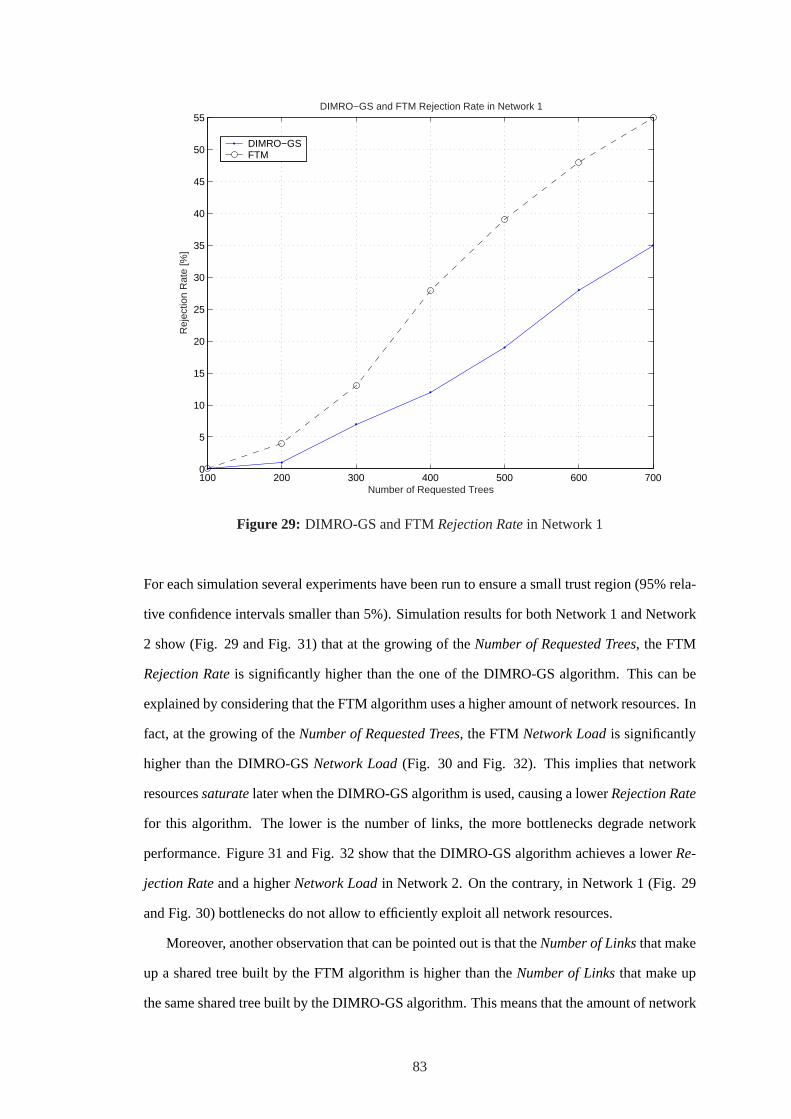
100 200 300 400 500 600 7000
5
10
15
20
25
30
35
40
45
50
55DIMRO−GS and FTM Rejection Rate in Network 1
Number of Requested Trees
Rej
ectio
n R
ate
[%]
DIMRO−GSFTM
Figure 29: DIMRO-GS and FTMRejection Ratein Network 1
For each simulation several experiments have been run to ensure a small trust region (95% rela-
tive confidence intervals smaller than 5%). Simulation results for both Network 1 and Network
2 show (Fig. 29 and Fig. 31) that at the growing of theNumber of Requested Trees, the FTM
Rejection Rateis significantly higher than the one of the DIMRO-GS algorithm. This can be
explained by considering that the FTM algorithm uses a higher amount of network resources. In
fact, at the growing of theNumber of Requested Trees, the FTMNetwork Loadis significantly
higher than the DIMRO-GSNetwork Load(Fig. 30 and Fig. 32). This implies that network
resourcessaturatelater when the DIMRO-GS algorithm is used, causing a lowerRejection Rate
for this algorithm. The lower is the number of links, the more bottlenecks degrade network
performance. Figure 31 and Fig. 32 show that the DIMRO-GS algorithm achieves a lowerRe-
jection Rateand a higherNetwork Loadin Network 2. On the contrary, in Network 1 (Fig. 29
and Fig. 30) bottlenecks do not allow to efficiently exploit all network resources.
Moreover, another observation that can be pointed out is that theNumber of Linksthat make
up a shared tree built by the FTM algorithm is higher than theNumber of Linksthat make up
the same shared tree built by the DIMRO-GS algorithm. This means that the amount of network
83

100 200 300 400 500 600 7000.1
0.2
0.3
0.4
0.5
0.6
0.7
0.8
0.9
1DIMRO−GS and FTM Network Load in Network 1
Number of Requested Trees
Net
wor
k Lo
ad [%
]
DIMRO−GSFTM
Figure 30: DIMRO-GS and FTMNetwork Loadin Network 1
400 600 800 1000 1200 1400 1600 18000
10
20
30
40
50
60DIMRO−GS and FTM Rejection Rate in Network 2
Number of Requested Trees
Rej
ectio
n R
ate
[%]
DIMRO−GSFTM
Figure 31: DIMRO-GS and FTMRejection Ratein Network 2
84

200 400 600 800 1000 1200 1400 1600 18000
10
20
30
40
50
60
70
80
90
100DIMRO−GS and FTM Network Load in Network 2
Number of Requested Trees
Net
wor
k Lo
ad [%
]
DIMRO−GSFTM
Figure 32: DIMRO-GS and FTMNetwork Loadin Network 2
resources used by the FTM algorithm is higher than the amount of network resources exploited
by the DIMRO-GS algorithm. At the growing of the group size, theNumber of Linksthat make
up the shared tree built by the proposed algorithm grows slower than theNumber of Linksthat
make up the shared tree built by the FTM algorithm, in both Network 1 and Network 2 (Fig.
33).
Figure 33 shows also that theNumber of Linksthat make up the shared tree built by the
DIMRO-GS algorithm is greater in the first network than in the second one. This is because
when the number of links in the network grows, the value of the exponent decreases. Thus,
paths built by the proposed algorithm are shorter, and theNumber of Linksthat make up the
shared tree is lower.
3.4.4 DiffServ DIMRO and DIMRO-GS Performance Evaluation
In this section we evaluate the performance of the DIMRO algorithm and the DIMRO-GS algo-
rithm integrated in a DiffServ network, and the simple case, not DiffServ integrated, in which a
group member/receiver cannot reuse the bandwidth exploited by another group member/receiver
with more stringent QoS requirements.
85

10 15 20 25 30 35 40 45 500
500
1000
1500
2000
2500
3000
3500
4000
DIMRO−GS and FTM average number of exploited links
Group Size [# of members]
Nun
ber
of e
xplo
ited
links
DIMRO−GS Network 1FTM Network 1DIMRO−GS Network 2FTM Network 2
Figure 33: DIMRO-GS and FTM average number of link
Network nodes are randomly placed on a Cartesian coordinate grid and links are generated
according to the probability function (63). Since we need to generate a DiffServ network, we
will consider the bandwidth capacity of a link for each service class. Let us consider a simple
DiffServ network with only four service classes that we indicate withA, B, C, D, whereA
is the highest service class andD is the lowest one. LetBuv(cl) be the bandwidth capacity
of link (u, v) for service classcl, cl ∈ A, B, C, D. The bandwidth capacityBuv(cl) for
each service class on link(u, v) is randomly generated by using an uniform distribution with
mean bandwidthB(cl). For this simulation campaign, a one hundred node network has been
randomly generated, with parametersα = 0.2 and β = 0.4, according to Tab I. The link
bandwidth capacity for each service classcl ∈ A, B, C, D is uniformly distributed with
mean bandwidthB(cl) equal to25 Mbps.
We consider theNetwork Loadas defined in (65) for each service class, when fifty source
rooted trees, randomly generated, are built by the DIMRO algorithm. Each receiver asks for
a rate uniformly distributed in the range[0.1, 2] Mbps, and a service class randomly selected
within the setA,B, C,D. Moreover, a 5 channel layering scheme is used, as described in
86

A B C D0
10
20
30
40
Service Class
Num
ber
of
R
ecei
vers
# 1
0
A B C D 0
10
20
30
40
Num
ber
of
R
ecei
vers
# 2
0
A B C D0
10
20
30
40
Num
ber
of
Rec
eive
rs #
30
DiffServ integratedNon DiffServ−integrated
Service Class
Service Class
Net
wor
k Lo
ad [%
]
Figure 34: DIMRO Network Load of DiffServ classes
Section 3.2.1.
For each simulation several experiments have been run to ensure a small trust region (95%
relative confidence intervals smaller than 5%). Figure 34 shows that DiffServ integrated DIMRO
performs better than its non integrated version. Furthermore, theNetwork Loaddecreases with
the service class. In particular, the lowest service classD has the lowestNetwork Loadbe-
causeD class receivers can reuse bandwidth already exploited by all other receivers. DiffServ
integrated DIMRO performs better than its non QoS-aware version, and this gets evident at the
growing of the number of receivers. Figure 34 shows that for 30 receivers theNetwork Loadfor
service classesB, C andD is significantly lower then theNetwork Loadrelative to these service
classes when DIMRO is not DiffServ integrated (theNetwork Loadis reduced respectively by
23%, 33% and 40%, as can be easily figured out from Fig. 34).
As far as concern the DIMRO-GS algorithm, we consider theNetwork Loadof each service
class when a multicast group is randomly generated and the DIMRO-GS algorithm is used to
build the corresponding shared tree. The group asks for a rate uniformly distributed in the range
[0.1, 2] Mbps, and each group member asks for a service class randomly selected within the set
A,B,C, D.
87
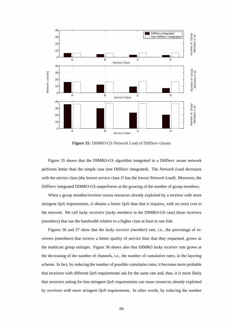
A B C D0
10
20
30
40
Service Class
Num
ber
of G
roup
Mem
bers
# 1
0
A B C D0
10
20
30
40
Service Class
Num
ber
of G
roup
M
embe
rs #
20
A B C D0
10
20
30
40
Service Class
Num
ber
of G
roup
Mem
bers
# 3
0
DiffServ integratedNon DiffServ−integrated
Net
wor
k Lo
ad [%
]
Figure 35: DIMRO-GS Network Load of DiffServ classes
Figure 35 shows that the DIMRO-GS algorithm integrated in a DiffServ aware network
performs better than the simple case (not DiffServ integrated). TheNetwork Loaddecreases
with the service class (the lowest service classD has the lowestNetwork Load). Moreover, the
DiffServ integrated DIMRO-GS outperforms at the growing of the number of group members.
When a group member/receiver reuses resources already exploited by a receiver with more
stringent QoS requirements, it obtains a better QoS than that it requires, with no extra cost to
the network. We calllucky receivers(lucky membersin the DIMRO-GS case) those receivers
(members) that use the bandwidth relative to a higher class at least in one link.
Figures 36 and 37 show that thelucky receiver (member) rate, i.e., the percentage of re-
ceivers (members) that receive a better quality of service than that they requested, grows as
the multicast group enlarges. Figure 36 shows also that DIMROlucky receiver rategrows at
the decreasing of the number of channels, i.e., the number of cumulative rates, in the layering
scheme. In fact, by reducing the number of possible cumulative rates, it becomes more probable
that receivers with different QoS requirements ask for the same rate and, thus, it is more likely
that receivers asking for less stringent QoS requirements can reuse resources already exploited
by receivers with more stringent QoS requirements. In other words, by reducing the number
88

5 10 15 20 25 30 35 40 45 50 5525
30
35
40
45
50
55
DIMRO Lucky Receiver Rate
Number of Receivers
Luck
y R
ecei
ver
Rat
e [%
]
3 CHANNEL LAYERING SCHEME5 CHANNEL LAYERING SCHEME
Figure 36: DIMRO Lucky Receivers
5 10 15 20 2530
35
40
45
50
55DIMRO−GS Lucky Member Rate
Group Size [# of members]
Luck
y M
emeb
er R
ate
[%]
Figure 37: DIMRO-GS Lucky Members
89

of channels, less receivers can obtain the desired rate, but more receivers attain a better QoS,
which means less losses, less retransmissions, and an increased throughput on the average.
3.5 Conclusions
DIMRO (DiffServ-Integrated Multicast algorithm for Internet Resource Optimization) and DIMRO-
GS (DiffServ-Integrated Multicast algorithm for Internet Resources Optimization in Group
Shared applications) algorithms, presented in this work, aim to avoid bandwidth bottlenecks
effectively, and to achieve an efficient distribution of link loads in the source rooted and group
shared multicast tree computation. The proposed multicast algorithms, seamless integrated into
the DiffServ Quality of Service approach, by leveraging their native multirate nature, efficiently
address the network partition problem. Both these multicast algorithms, embedded with a novel
low computational cost multirate layering algorithm to effectively accommodate heterogeneous
receiver requested rates, have been described and tested in an integrated DiffServ aware network
through extensive C++ based simulations. The simulation results show a better leverage of the
network bandwidth resources and an improved QoS perceived by multicast group members with
respect to the performance of existing multicast algorithms. Moreover, the low computational
complexity which characterizes all the proposed algorithms, effectively leads to time and re-
source saving.
90

CHAPTER IV
MOBILE AD HOC NETWORKS (MANET)
4.1 The Notion of “Ad Hoc Network”
A Mobile Ad Hoc Network (MANET) is a network architecture that can be rapidly deployed
without relying on pre-existing fixed network infrastructure. The nodes in a MANET can dy-
namically join and leave the network, frequently, often without warning, and possibly without
disruption to other nodes’ communications. In addition, nodes in a ad hoc network can be highly
mobile. Thus, the node constellation and the presence or absence of links can rapidly change.
Examples of possible applications for MANETs are:
• Tactical operations, for fast establishment of military communications during the deploy-
ment of forces in unknown and hostile terrain;
• Rescue missions, for communication in areas without adequate wireless coverage;
• National security, for communications in times of national crisis, where the existing com-
munication infrastructure is non-operational due to a natural disaster or a global war;
• Law enforcement, for fast establishment of a communication infrastructure during law
enforcement operations;
• Commercial use, for quickly setting up communications in exhibitions, conferences, or
sale presentations;
• Education, for operation of wall-free (virtual) classrooms;
• Sensor networks, for communications among sensors which monitor an area and sense
the environment for event occurrence.
Nodes in a MANET exhibit nomadic behavior by freely migrating within the terrain, dy-
namically creating and tearing down associations with other nodes. Groups of nodes that have
a common goal can create formations (clusters) and migrate together, similarly to military units
on missions or to guided tours on excursions. Nodes can communicate with each other at any
91

time and without restrictions, except for connectivity limitations and/or limitations due to se-
curity provisions. Examples of network nodes are pedestrians, soldiers, sensors, or unmanned
robots. Examples of mobile platforms on which network nodes might reside are cars, trucks,
buses, tanks, trains, planes, helicopters, or ships.
MANETs are intended to provide a data network that is immediately deployable in arbi-
trary communication environments and is responsive to changes in network topology. Because
ad hoc networks are intended to be deployable anywhere, existing infrastructure may not be
present. The mobile nodes are thus likely to be the sole elements of the network. Differing
mobility patterns and radio propagation conditions that vary with time and position can result
in intermittent and sporadic connectivity between adjacent nodes. The result is a time-varying
network topology. MANETs are distinguished from other ad hoc networks by rapidly changing
network topologies, influenced by the network size and node mobility. Such networks typically
have a large span and contain hundreds to thousands of nodes. MANET nodes exist on top of
diverse platforms that exhibit quite different mobility patterns. Within a MANET, there can be
significant variations in node speed (from stationary nodes to high-speed aircraft), direction of
movement, acceleration/deceleration or restrictions on paths (e.g., cars must drive on a road,
but tanks do not). A pedestrian is restricted by built objects while airborne platforms can exist
anywhere in some range of altitudes. In spite of such volatility, MANETs are expected to deliver
diverse traffic types, ranging from pure voice to integrated voice and image, and even possibly
some limited video.
4.2 The Communication Environment and the MANET Model
The following are a number of assumptions about the communication parameters, the network
architecture, and the network traffic in a MANET.
• Nodes are equipped with portable communication devices. Lightweight batteries may
power these devices. Limited battery life imposes restrictions on the transmission range,
communication activity (both transmitting and receiving) and computational power of
these devices.
• Connectivity between nodes is not a transitive relation, i.e., if nodeA can communicate
directly with nodeB and nodeB can communicate directly with nodeC, then nodeA
92

may not be able to communicate directly with nodeC. This leads to the hidden termi-
nal problem [149]. Moreover, links are likely to be asymmetrical, i.e., if nodeA can
communicate with nodeB, nodeB may not be able to communicate to nodeA.
• A hierarchy in the network routing and mobility management procedures could improve
network performance measures such as latency in locating a mobile. However, a physical
hierarchy may lead to areas of congestion and is very vulnerable to frequent topological
reconfigurations.
• Nodes are generally assumed to be identified by fixed identification numbers, i.e., IDs
(e.g., based on IP addresses [125]).
• All the network nodes have equal capabilities. This means that all nodes are equipped
with identical communication devices and are capable of performing functions from a
common set of networking services. However, all nodes do not necessarily perform the
same functions at the same time. In particular, nodes may be assigned specific functions
in the network, and these roles may change over time.
• Although the network should allow communication between any pair of nodes, it is envi-
sioned that a large portion of the traffic will be among geographically close nodes. This
assumption is clearly justified in a hierarchical organization. For example, it is much more
likely that communication will take place between two soldiers in the same unit, rather
than between two soldiers in two different brigades.
A MANET is a peer-to-peer network that allows direct communication between any two
nodes, when adequate radio propagation conditions exist between these two nodes. If there
is no direct link between the source and the destination nodes, multi-hop routing is used. In
multi-hop routing, a packet is forwarded from one node to another, until it reaches the destina-
tion. Clearly, appropriate routing protocols are necessary to discover routes between the source
and the destination, or even to determine the presence or absence of a path to the destination
node. Because of the lack of central elements, distributed protocols have to be used. The main
challenges in the design and operation of MANETs, compared to more traditional wireless net-
works, stem from the lack of a centralized entity, the potential for rapid node movement, and the
fact that all communication is carried over the wireless medium. In standard cellular wireless
93

networks, there are a number of centralized entities (e.g., the Base Stations (BS), the Mobile
Switching Centers (MSCs), the Home Location Register (HLR), and the Visitor Location Reg-
ister (VLR)). In ad hoc networks, there is no preexisting infrastructure, and these centralized
entities do not exist. The centralized entities in the cellular networks perform the function of
coordination. The lack of these entities in MANETs requires distributed algorithms to perform
these functions. In particular, the traditional algorithms for mobility management, which rely
on a centralized HLR/VLR, and the medium access control (MAC) schemes, which rely on the
BS/MSC support, become inappropriate. All communications between all network entities in
ad hoc networks are carried over the wireless medium. Due to the radio communications being
vulnerable to propagation impairments, connectivity among network nodes is not guaranteed.
In fact, intermittent and sporadic connectivity may be quite common. Additionally, since the
wireless bandwidth is limited, its use should be minimized. Finally, since some of the mo-
bile devices are expected to be hand-held with limited power sources, the required transmission
power should be minimized as well. Therefore, the transmission radius of each mobile is lim-
ited, and channels assigned to mobiles are typically spatially reused. Consequently, since the
transmission radius is much smaller than the network span, communication between two nodes
often needs to be relayed through intermediate nodes, i.e., multi-hop routing is used.
Because of the possibly rapid movement of the nodes and variable propagation conditions,
network information such as a route table, becomes obsolete quickly. Frequent network recon-
figuration may trigger frequent exchanges of control information to reflect the current state of
the network. However, the short lifetime of this information means that a large portion of this
information may never be used. Thus, the bandwidth used for distribution of the routing update
information is wasted. For these reasons, the design of MANETs needs to allow for a high
degree of reliability, survivability, availability, and manageability of the network.
Based on the above discussion, the following features for MANETs are required:
• Robust routing and mobility management algorithmsto increase the network’s relia-
bility and availability, e.g., to reduce the chances that any network component is isolated
from the rest of the network;
• Adaptive algorithms and protocols to adjust to frequently changing radio propagation,
network, and traffic conditions;
94

• Low-overhead algorithms and protocolsto preserve the radio communication resource;
• Multiple (distinct) routes between a source and a destination to reduce congestion in the
vicinity of certain nodes, and to increase reliability and survivability;
• Robust network architecture to avoid susceptibility to network failures, congestion
around high-level nodes, and the penalty due to inefficient routing.
The ad hoc networking technology has stimulated substantial research activity in the past
10 years. The rather interesting fact is that although the military has been experimenting and
even using this technology for the last three decades, the research community has been coping
with the rather frustrating task of finding a ‘killer’ non-military application for ad hoc networks.
A major challenge that has been perceived as a possible ‘show stopper’ for technology transfer
is the fact that commercial applications do not necessarily conform to the ‘collaborative’ en-
vironment that the military communication environment does. In other words, why should a
user forward someone else’s transmission, depleting her own battery power and, thus, possibly
restricting her use of the network in the future? This question may relate to the issue of billing
- if billing is possible (and, in fact, desirable), then nodes that serve as ‘good citizens’ could be
rewarded. But billing is, by itself, a significant challenge in ad hoc networks.
Other challenges in deployment of ad hoc networks relate to the issues of manageability,
security, and availability of communication through this type of technology. Realizing that
technology transfer has not been the motivating factor, the recent research interest in ad hoc net-
works could be, most probably, attributed to the intellectual challenges that are part of this type
of communication environment. Nevertheless, we believe that there is substantial commercial
potential of ad hoc networks. Future extensions of the cellular infrastructure could be carried out
using this type of technology and may be the basis for fourth generation (4G) of wireless sys-
tems. Other possible applications include sensing systems (also referred to as Sensor Networks)
or augmentation to the wireless LAN technology.
4.3 A Promising Application: “Sensor Networks”
Sensor networks [12] differ from “traditional” ad hoc networks in many aspects. The number of
nodes in a sensor network can be several orders of magnitude higher than in ad hoc networks,
and the deployment of nodes is usually denser. Moreover, sensor nodes are limited in power,
95

computational capacities and memory, and they may not haveglobal identification(ID) because
of the very large number of nodes and the related overhead.
Due to the above constraints, sensor network protocols and algorithms must be endowed
with self-organizing capabilities, i.e., sensors must be able to cooperate in order to efficiently
perform networking tasks. The primary design constraints of these algorithms areenergy effi-
ciency, scalabilityandlocalization.
It has been recently pointed out [78] that energy efficiency in mobile systems can be im-
proved by designing protocols and algorithms with across-layer approach, i.e., by taking into
account interactions among different layers of the communication process so that the overall en-
ergy consumption can be minimized. Hence, interdependencies between physical and network
layer functionalities to improve the energy efficiency of the routing tasks should be considered.
A primary requirement of configuration algorithms for large scale ad hoc networks, such
as routing algorithms, isscalability, i.e., these algorithms should perform well for wireless
networks with an arbitrary number of nodes. The notion of scalability is strictly related to that
of localization: in a scalable algorithm each node exchanges information only with its neighbors
(localizedinformation exchange) [59]. In alocalized routing algorithm, each node selects the
next hop based only on the position of itself, of its neighbors, and of the destination node. As a
result, the local routing decision of each node strives to achieve a global network objective such
as minimum latency or minimum energy consumption. Conversely, in a non-localized routing
algorithm a node maintains an accurate description of the overall network topology to select the
next hop. This way, the routing problem is equal to the shortest path problem if thehop count
is used as the global performance metric or the shortest weighted path ifpower [129] or cost
[155][41] link metrics are used.
It has been shown [102][91] that routing protocols that do not use geographical location
information are not scalable, e.g., AODV (Ad hoc On-demand Distance Vector), DSDV (Desti-
nation Sequenced Distance Vector) or DSR (Dynamic Source Routing). On the other hand, the
recent availability of small, inexpensive and low-power GPS (Global Positioning System) re-
ceivers, together with techniques to deduce relative sensor coordinates from signal strengths [84]
encourage researchers to developGeographical Routing[144] (alsoPosition Based Routing) al-
gorithms, which are deemed to be the most promising solutions for critically power-constrained
ad hoc networks.
96

In [112] the authors deal with the interdependencies between topology control [127] and en-
ergy efficient geographical routing. The question they try to answer is“How extensive should be
the Local Knowledge of the global topology in each node, so that energy efficient geographical
routing decisions can be taken?”. The answer to the question is clearly related to the “degree”
of localization of the routing scheme. If each node could hold a complete vision (knowledge)
of the network topology, it could then compute the “globally” optimal next hop, i.e., the neigh-
boring node on the minimum energy path. However, acquiring increasingly accurate topology
information has an increasing cost, i.e., the energy required to exchange the signaling traffic that
convoys this information.
Hence, in [112] the authors develop an analytical framework to capture the trade-off between
what they refer to as thetopology information cost, which increases with increasing range of
knowledge of each node, and thecommunication cost, which may decrease when the knowledge
becomes more complete. They apply this analytical framework to different position based for-
warding schemes [146][87][63][98][117] and show by Monte Carlo simulations that a limited
knowledge is sufficient to make energy efficient routing decisions. With respect to the existing
literature on geographical routing, they try to better define the terms “localized” and “neighbor”.
A “neighbor” for a certain node is another node which falls into itsTopology Knowledge Range,
denoted as KR. To summarize, the main contributions of [112] are:
• Introduction of ananalytical frameworkto evaluate the energy consumption of geograph-
ical routing algorithms for power constrained large scale ad hoc networks;
• Development of an Integer Linear Programming (ILP) formulation of thetopology Knowl-
edge Rangeoptimization problem;
• Detailed comparison of the leading existing forwarding schemes and introduction of a
new scheme calledPartial Topology Knowledge Forwarding(PTKF);
• Introduction of aPRobe-bAsed Distributed protocol for knowledge rAnge adjustment
(PRADA), that allows each node to efficiently select online its topology knowledge range.
PRADA is shown to lead to near-optimal energy consumption.
97

4.4 Mobility Model Introduction
The movement pattern of users plays an important role in performance analysis of mobile and
wireless networks. In cellular networks, for example, a user’s mobility behavior directly af-
fects the signaling traffic needed for handover and location management (location updates and
paging) [58]. The extra signaling messages over the air interface consume radio resources and
increase the associated database query load. In addition, mobility has a major effect on the
channel holding time in circuit-switched services [85][76][119][62]. The latter has in turn huge
influence on the call blocking and dropping probability [105]. The modeling of movement is
thus an essential building block in analytical and simulation-based studies of these systems.
Mobility models are needed in the design of strategies for location updating and paging, ra-
dio resource management (e.g., dynamic channel allocation schemes), and technical network
planning and design (e.g., cell and location area layout, network dimensioning).
The choice of the mobility model has a significant effect on the obtained results. If the model
is unrealistic, invalid conclusions may be drawn. With the increasing number of subscribers and
the decreasing cell size in future cellular systems, the mobility pattern of users will even more
influence the performance of the network. Models that proved to be a good choice in simulation
of macro-cellular environments show some drawback when being applied in micro- and pico-
cellular environments [137]. Mobility modeling also plays an important role in analysis of
algorithms and protocols in wireless local area networks (WLANs) and self-organizing wireless
ad hoc networks. Whereas in cellular networks there exists a number of approaches that model
the macroscopic movement behavior of users (e.g., random walk from cell to cell, description
of the cell residence time), in these cases we need a “microscopic” model.
4.5 Mobility Model Overview
There exists a variety of mobility models that find application in different kinds of simulations
and analytical studies of wireless systems. Figure 38 shows a concept map illustrating some cri-
teria which can be used for categorization. Analytical mobility models are, in general, based on
rather simple assumptions regarding the movement behavior of users, but they allow the calcu-
lation of mathematical expressions with respect to system performance. Several authors derive
the distribution of a user’s cell residence time [85][160][161][115]. For example, in [160] it is
shown that the cell residence time with their model can be described by a generalized gamma
98

bounce back
wrap-around
delete and replace
Borderbehaviourmodel
never
predefined
probabilistic
when tochangespeed
changespeedmethod
changespeedmodel
choose direction
choosedestination
choose pointnever
predefined
probabilistic
when tochangedirection
changedirectionmethod
changedirectionmodel
randommobilitymodel
eventtriggeredmovement
simulation
timedomanin
deterministicapproach
hybridapproach
degree ofrandomness
dimension
MobilityModel
aggregatedmovementbehaviour
randomwalk
individualusers
level ofdetail
application
analyticaldescription
1D
micromobility
realmobilitytrace
street, officemovementbounded byenvironment
spacedomanin
macromobility
2D
3D
fluid flow
gravity \transport
Figure 38: Concept map of mobility models used in simulation and analysis of wireless com-munication systems
distribution. Combining these “mobility metrics” with traffic models allows to estimate impor-
tant system performance parameters, such as channel holding time and handover and location
update events [85][76][160]. For example, in [85] the authors analyze the mean handover rate
for voice calls. In [76] is derived a distribution for the channel holding time. In [160] is also de-
rived a distribution for the channel holding time and the average number of handovers per call.
Let us briefly describe the mobility assumptions used by these authors. In [85] they assume that
mobile users are uniformly distributed over a cell. Each user chooses a directionφ (taken from
a uniform distribution in[0, 2π]) and a speedv (uniformly distributed in the interval[0, Vmax]).
Once these values are chosen, they remain constant until the user crosses the boundary of the
cell. In [76] it is exploited a more general model, in which direction changes are also possible
within a cell. The model in [160] allows direction changes only to a certain extent (∆φmax).
The authors in [106][61] assume a generally distributed location area residence time as
given. From this, they derive the probability distribution of the number of location area crossings
for a given distribution of the interservice time (i.e., the time between the beginning of two
unblocked calls). Another analytical model is the Brownian mobility model, which models
the movement of users based on Brownian motion such that we can calculate the probability
99

distribution of the physical location of a user at given timet, provided that we know her location
at a previous timet0 < t. Models used for simulation-based studies describe movement of users
in a more detailed manner. On the other hand, in general, they do not allow the derivation of
analytical expressions.
For example, the European Telecommunications Standards Institute (ETSI) defined a set
of test scenarios for system simulation of UMTS (Universal Mobile Telecommunication Sys-
tem). The document [60] describes mobility models for three environments: an indoor office, an
outdoor pedestrian environment, and a vehicular environment. The model for the pedestrian en-
vironment uses a Manhattan-like street structure rectangular grid. Pedestrians walk along streets
in a straight line and can change their direction at intersections with a given probability. Also
speed changes are possible after given intervals. The model for the vehicular environment is a
random mobility model with a street structure. Cars move with constant speed(v = 120km/h)
and can change their direction every20 m (with a probability of20%). Only direction changes
of up to±45 are possible.
In [37] the ETSI model is extended to get more realistic results. They analyze mobility-
related parameters of their model such as the cell residence time and the cell boundary crossing
rate, and compare it to the ETSI model.
Let us now consider the different levels of detail in mobility modeling (see Fig. 38). Re-
searchers in vehicular traffic theory distinguish between three levels of description:microscopic,
mesoscopic (kinetic), andmacroscopic. A microscopic model describes the movement of a sin-
gle vehicle by its space and speed coordinates at a given timet. Such approaches include very
detailed “car following” models. At mesoscopic level, the homogenized movement behavior of
several vehicles is reflected. For example, a distribution function is derived that describes the
number of vehicles at a certain location(x, y) or speedv at timet. When modeling on a macro-
scopic scale, one is interested in high level statistical characterizations, e.g., the density, mean
speed and speed variance, and traffic flow of vehicles. An example for a macroscopic movement
model used in analysis of wireless systems is the fluid flow model [148]. This family of analyti-
cal models describes the mobility in terms of “the mean number of users crossing the boundary
of a given area”. A second approach used for modeling the macroscopic movement behavior
is the family of gravity models [99]. They are also derived from transportation theory. Such
models give an aggregated description of the movement of several users (as the fluid model),
100

ranging from city scale to international scale. The authors in [109] describe such a model. They
use the concept of trips, area and time zones, population groups, and so on. The paper [142] also
falls into this category. It models the daily movement of users which follow an activity-based
travel demand model.
Another frequently used approach in cellular networks is the family ofrandom walk models,
also denoted as Markovian mobility models. They describe movement of individual users from
cell to cell. The exact location of a user is of interest but just the cell in which she resides.
The model is basically defined by a state-transition diagram in which a cell is represented by
a state and the movements between cells by transition probabilities between the states. A user
either stays within her cell or moves to one of its neighboring cells with a certain probability.
A typical random walk model in one dimension is described in [6]. Two dimensional random
walk models are used in [10][47][141]. Recent enhancements include a random walk model
presented in [11]. From these models, we can also derive analytical measures for the crossing
rates of cell and location area boundaries.
Wireless researchers also invented models for three timensional movement. The authors in
[96] model user movements inside buildings, including vertical movements in staircases and
elevators. There exists a variety of generalizations of the model in [76] which are used in
simulation-based studies of wireless systems. Basically, this class of mobility models can be
described by the following paradigm: users can move freely anywhere in the system area. The
values for the user directionφ are uniformly distributed in[0, 2π], i.e., users do not have any
preferred direction. The speed valuesv is usually assigned a uniform or a normal distribution.
After a randomly chosen time, usually with an exponential distribution, a user chooses a new
direction. The same procedure is performed for speed changes. The stochastic processes for
direction and speed change are in general correlated to each other. A node is thereby completely
described by its current space vector(x(t), y(t)), its current speedv(t), and its current direction
φ(t), where the following constraints generally hold:0 ≤ x(t) ≤ xmax, 0 ≤ y(t) ≤ ymax,
0 ≤ v(t) ≤ Vmax, and0 ≤ φ(t) ≤ 2π ∀t. This is also referred to as random direction mobility
model.
In [80][121], it is used a simplified version of the random direction model. All users always
have the same constant speedvo and move with an initial directionφo picked in the interval
[0, 2π] with a uniform distribution. When a user reaches the border of the simulation, it changes
101

its direction, “bouncing” back with a new direction angleφ = π − φo.
Another random mobility model is the random waypoint model, which is used by several
authors in the ad hoc networking community [39][132][49][50][94]. According to this mobility
model, a user randomly chooses a destination point in the system area, moves on a straight line to
this point with constant speedv (chosen in the interval[Vmin, Vmax] with a uniform distribution),
and pauses for a certain time before it again chooses a new destination. This model is very
similar to a generalized random direction model. The difference is that the destination point is
chosen rather than the directionφ. A node is described by its current space vector(x(t), y(t)),
its current speedv(t), and its current destination point(Xd(t), Yd(t)).
Let us now consider the “degree of randomness” different mobility models have (see Fig.
38). Basically, a mobility model belongs to one of the three following cases:
1. Users can move anywhere in the system plane following a pseudo-random process for
speed and direction;
2. Users are bound by streets, buildings, and so on, but use a pseudo-random process for
speed and direction choice at crossings;
3. Users are bound to a defined path.
We already gave many examples for the first case, the random waypoint and the random di-
rection model being only two of them. ETSI in-house and pedestrian outdoor models with
simple Manhattan-like street structure is an example for the second type. Such models are also
described in detail in [109].
A deterministic approach for simulations would allow users to move only on a predefined
mobility path, which is the third case for mobility models. Such a path can describe typical
movement patterns of pedestrians and vehicles. We can further distinguish two cases. In the
first case, the direction and speed are both given, and no random process is incorporated at
all. In the second case, the direction trace is given but the speed is chosen randomly. Such
traces can exist in different levels of detail (cells, areas, etc.). In [99] the authors describe a
family of macroscopic mobility models based on traces. Nevertheless, in practice, tracing the
actual mobility behavior of users is a very complicated and resource-draining task and usually
such information is hard to obtain by network providers. Thus, researchers often use random
102

models. Moreover, privacy issues including the confidentiality of certain data, may prohibit the
collection and distribution of such statistics.
4.6 Cellular Mobility Models
Cellular mobility models focus their attention on individual movements since key issues often
involve paging and hand-offs of a single user or MN (Mobile Node). Rarely do more compli-
cated issues such as group management come into play. As a result, mobility models such as
the following were developed to test the behavior of cellular protocols and strategies:
1. Random Walk Model;
2. Constant Velocity Fluid-Flow Model;
3. Random Gauss-Markov Model.
4.6.1 Random Walk Mobility Model
The Random Walk Mobility Model has been proven to be one of the most widely used mobility
models because it describes individual movements relative to cells [161][6][133]. Many entities
in nature move in extremely unpredictable ways. Molecules, for example, move in random
directions, i.e., they do not yield a pattern or sense of direction [143]. The random walk was
developed in an attempt to mimic the erratic movements of certain objects. Specifically, in the
Random Walk Mobility Model, a host moves from its current location to a new location by
randomly choosing a direction and speed. The new speed and direction are both chosen from
pre-defined ranges,[vmin, vmax] and [0, 2π] respectively. Each movement in the Random Walk
Mobility Model occurs in a constant time interval, at the end of which a new direction and speed
are calculated. Many derivatives of the Random Walk Mobility Model have been developed
including the one-dimensional, two-dimensional, three-dimensional, and d-dimensional walks.
We mention only the 1-D and 2-D walks, since the 3-D and d-D walks may easily be extrapolated
from those.
In a 1-D walk, we imagine a gymnast standing in the middle of an infinitely long balance
beam. Given the results of a coin flip, the gymnast moves in a particular direction at a random
speed for a certain amount of time. For example, if the coin flip results in heads, the gymnast
moves to the right at the randomly chosen speed. In contrast, if the coin flip results in tails, the
103

gymnast moves to the left. After repeating this pattern for a large number of times, a 1-D walk
is mapped.
In a 2-D walk, we visualize the same gymnast moving on a planar surface. For example,
using a similar method as that mentioned in the 1-D walk, we generate a 2-D random walk.
Specifically, instead of visualizing a gymnast on a balance beam we expand our environment
to include an infinite floor. Instead of flipping a coin, the gymnast uses a spinning dial. After
spinning the dial, the gymnast moves in the direction pointed to by the needle at a random speed
for a certain amount of time. In doing so, the gymnast randomly moves around a 2-D surface,
thus creating a 2-D walk.
In 1921 Polya proved that a random walk on a one- or two-dimensional lattice returns to the
origin with complete certainty, i.e., with a 1 probability [153]. This characteristic ensures that
the random walk accurately represents a mobility model that emulates the movements of entities
around their starting points. The two-dimensional walk is of special interest to researchers
developing protocols for cell-related technologies, since the Earth’s surface is modelled using
a two-dimensional representation. Unfortunately, the simplicity of the Random Walk Mobility
Model is not always sufficient to produce realistic results. Figure 39 shows an example of
the movement observed using a 2-D model. The Mobile Node (MN) begins its movement at
position (0,0). At each point, the MN randomly chooses a direction between 0 and2π and
a speed between 0 and10 m/s. The MN is allowed to travel for a total of1 second before
changing direction and speed. It is easy to note the restricted behavior of the Random Walk
Mobility Model, proven by Polya. The node illustrated in Fig. 39 rarely travels far from the
origin.
In a special case of the Random Walk Mobility Model, a MN no longer travels for a con-
stant time period before changing direction. Instead, a MN changes direction after travelling a
specified distance. Figure 40 illustrates an example of the movement observed according to this
modified mobility model. We note that the figure only illustrates a small region of a200× 200
simulation area. A MN begins its movement in the middle of the simulation area (e.g., at posi-
tion (0,0)). At each point the MN randomly chooses a new direction between0 and2π and a
speed between0 and10m/s. The MN travels for a total of10 units before changing its direction
and speed.
The Random Walk Mobility Model is amemorylessmobility pattern because it retains no
104

-600
-600
600
600-600
-600
600
600-600
-600
600
600
Figure 39: Travelling pattern of a Mobile Node (MN) using the 2-D Random Walk MobilityModel
Figure 40: Travelling pattern of a Mobile Node (MN) using the modified 2-D Random WalkMobility Model
105

knowledge concerning its past locations and speed values. This characteristic inhibits the prac-
ticality of the Random Walk Mobility Model because MNs typically have a pre-defined desti-
nation and speed in mind, which in turn affects future destinations and speeds. Other mobility
models such as the Random Gauss-Markov Mobility Model attempt to fix this discrepancy.
4.6.2 Fluid-Flow Mobility Model
Fluid mobility models describe macroscopic movements instead of individual or microscopic
movements. The behavior of the generated traffic is similar to a fluid flowing through a pipe. As
a result, the Fluid-Flow Mobility Model best represents traffic on highways and other similar sit-
uations with a constant flow of MNs. In other words, the model is unable to accurately represent
the movements of individual MNs. As an example, a deterministic Fluid-Flow Mobility Model
is used in [101] to represent the behavioral characteristics of traffic on a one-way, semi-infinite
highway. Cars enter and exit the highway at various locations. Haas and Liang [79] confirm that
the Fluid-Flow Mobility Model is insufficient for individual movements including stopping and
starting, actions commonly associated with an individual walking around town or from class to
class.
4.6.3 Random Gauss-Markov Mobility Model
The Random Gauss-Markov Mobility Model was introduced in order to circumvent the unde-
sirable results mentioned above with reference to [79]. In the Random Gauss-Markov Mobility
Model, the velocity of a MN at timen is given by the equation
νn = ανn-1 + (1− α)µ +√
1− α2 · xn-1 (67)
whereα is the tuning parameter used to vary the randomness,µ is a constant representing the
mean value ofνn asn →∞, andxn-1 is a random variable from a Gaussian distribution. Totally
random values are obtained by settingα = 0 and linear motion is obtained by settingα = 1.
Intermediate levels of randomness may be obtained by varying the value ofα between0 and1.
The displacement of a MN is given by the equation
sn =n-1∑
i=0
νi (68)
By allowing past velocities and directions to influence future velocities and directions, the Ran-
dom Gauss-Markov Mobility Model solves the problems encountered in the Random Walk Mo-
bility Model. This way, it also allows studying individual MN movements, thus overcoming the
106

problems encountered in the Fluid-Flow Mobility Model.
4.7 Ad Hoc Mobility Models
In ad hoc wireless mobile networks, the mobility models focus on the individual motion be-
havior between mobilityepochs, which are the smallest time periods in a simulation in which a
mobile host moves in a constant direction at a constant speed. Many researchers use the Ran-
dom Mobility Model [161][138]. According to this model, the speed and direction of motion
in a new time interval have no relation to their past values in the previous epoch. This model
can generate unrealistic mobile behavior such as sharp turning or sudden stopping. Some au-
thors use modified versions of the random mobility model. In [23], the author describes the
movement of MNs in their simulation for the DREAM (Distance Routing Effect Algorithm for
Mobility) protocol such that a MN has a random direction at every simulation clock tick, but
a constant speed during the entire simulation period. The mobility model in [97] for the LAR
(Location-Aided Routing) routing protocol allows MNs to move along a path which is made up
of several segments. The segment lengths are exponentially distributed and the direction of each
segment is randomly chosen. Speed is uniformly distributed in[v − α, v + α].
In the model proposed in [48], a node chooses its speed, direction and distance based on a
pre-defined distribution, then calculates its next destination and the time to reach it. When the
node reaches that point, it calculates a new destination and time period to reach it again. The
Random Waypoint mobility model [95] is also an extension of random walk. This model breaks
the entire movement of a MN into repeating pause and motion periods. A mobile host first stays
at a location for a certain time, then it moves to a new random-chosen destination at a speed
uniformly distributed in[0, vmax].
In [43], a Markovian model is used to describe the random motion. States represent motion
directions. The probability of maintaining the current state (or moving to another state) is spec-
ified in the transit matrix. Once in motion, the MN is more likely to keep on going at the current
direction and speed. This model is more realistic than the random model. Similar to [43], other
models [161][77] consider the relationship between a mobile host’s previous motion behavior
and the current movement characteristics such as speed and/or direction. In particular, the author
in [77] presents an incremental model in which, after each time increment, speed and direction
of current movement randomly diverge from the previous speed and direction, respectively. In
107

particular, speedv(t) and directionθ are expressed as below,
v(t + ∆t) = min[max[v(t) + ∆v; 0]; vmax] (69)
θ(t + ∆t) = θ(t) + ∆θ (70)
where∆v and∆θ are uniformly picked in reasonable ranges, e.g.,[−Amax∆t, Amax∆t] and
[−α∆t, α∆t], respectively, beingAmax the unit acceleration/deceleration andα the maximal
unit angular change.
Further, in [138], the author studies the relationship among MNs. This relationship exists
while MNs move with the same purpose. As can be noticed in a disaster recovery mission, or in a
military setting, several mobile hosts most likely move with a common objective. Two examples
given in [138] are thePursuemodel, where MNs try to move towards a target, and theColumn
model, which represents a searching activity. These models try to capture the interdependencies
among nodes in their movements, whereas most existing cellular and ad hoc wireless mobility
models describe independent node motion behavior.
Ad hoc mobility models differ from cellular mobility models in the network they model.
Cellular mobility models require the use of BSs whereas ad hoc mobility models require the
cooperation of two or more communicating MNs. Although separate mobility models exist
for cellular and ad hoc mobility models, similarities exist between the two categories. In the
following of this section we describe the most popular ad hoc mobility models.
4.7.1 Random Mobility Model
The Random Mobility Model for ad hoc networks coincides with the Random Walk Mobility
Model for cellular networks. In the Random Mobility Model, the current speed and direction
of a MN are both random variables that have no correlation with their current values [86].
Thus, we encounter an unrealistic choppy motion with sudden stopping, sharp turning, and
completely random wandering. In order to avoid these problems, many authors modified the
Random Mobility Model by changing the calculation of speed, direction, or both.
4.7.2 Constant Velocity Random Direction Mobility Model
Constant Velocity Random Direction Mobility Model [23][86] revised the Random Mobility
Model to ensure that every node is assigned the same speed throughout the entire simulation.
After a random direction is chosen in the range[0, 2π], a MN begins moving. If the MN reaches
108

a grid boundary, it bounces on the simulation border with an angle determined by the incoming
direction. The MN then continues along this new path.
4.7.3 Random Waypoint Mobility Model
The Random Waypoint (RWP) Mobility Model used in [95] includes pause times between
changes in direction and/or speed. In this stochastic model, each node of the network randomly
chooses a destination point, i.e., ‘waypoint’, in a rectangular deployment regionQ. A node
moves to this destination with a velocityv uniformly chosen in[vmin, vmax]. When it reaches
the destination, it remains static for a predefined pause timetp and then starts moving again
according to the same rule.
It has been observed in several papers [132][27][29][31][36] that the spatial distribution of
nodes moving according to the RWP model is non uniform. Although the initial node position-
ing is typically taken from a uniform random distribution, the mobility model changes this dis-
tribution during the simulation. This effect, known as border effect [27], occurs because nodes
tend to cross the center ofQ with a relatively high frequency. For a long running time of the
movement process, the stochastic distribution of the nodes converges toward an asymptotically
stationary distribution with the maximum node density in the middle ofQ. The non-uniformity
of the RWP node distribution has important practical consequences.
First, it reduces the applicability of existing analytical results concerning ad hoc networks,
which are typically based on the uniformity assumption. For example, theoretical results with
respect to routing [16][116], capacity [71][74], connectivity [28][75][140], and minimum power
issues cannot be applied directly in a mobile scenario that employs the RWP model.
Second, the nonuniform distribution implies that the representativeness of the huge amount
of simulation results obtained by using the RWP model could be impaired. This is because the
short-term behavior of the RWP model is quite different from the actual long-term behavior. In
[122] a modified version of the Random Waypoint Mobility Model is proposed so that a MN
travels at a constant speed throughout the entire simulation.
In [30], a generalized version of the RWP model is proposed. In this generalized model, a
node may remain static for the entire simulation time with a given probability. Hence, only a
fraction of the nodes are expected to move. Also, the model considers the fact that nodes are
initially deployed according to an arbitrary spatial distribution. The pause timetp is allowed to
109

Figure 41: Travelling pattern of a Mobile Node (MN) using the Random Waypoint MobilityModel
be different after each movement period. Figure 41 shows an example of travelling pattern of a
MN using the Random Waypoint Mobility Model starting at a randomly chosen point. We note
that the movement pattern of a MN using the Random Waypoint Mobility Model is similar to the
Random Walk Mobility Model if pause time is zero and the velocity interval ranges coincide,
i.e., [0, vmax] =[vmin, vmax].
4.7.4 Random Direction Mobility Model
The Random Direction Mobility Model [131] was developed in order to overcome a flaw dis-
covered in the Random Waypoint Mobility Model. MNs using the Random Waypoint Mobility
Model often choose a new destination that is located in the center of the simulation area, or that
requires travelling through the middle of the simulation area. In [131] it is stated that MNs mov-
ing with the Random Waypoint Mobility Model appear to converge, disperse, converge again,
etc. In order to alleviate this type of behavior and promote a semi-constant number of neighbors,
the Random Direction Mobility Model was developed. In this model, MNs choose a random
direction rather than a random destination. After choosing a random direction, a MN travels to
the border of the simulation area in that direction. As soon as the boundary is reached the MN
110

Figure 42: Travelling pattern of a Mobile Node (MN) using the Random Direction MobilityModel
stops for a certain period of time, chooses another angular direction in[0, π] and continues the
process. Figure 42 shows an example path of a MN, which begins at the center of the simulation
area, i.e., at(250, 250), using the Random Direction Mobility Model. A slight modification
to the Random Direction Mobility Model is the Modified Random Direction Mobility Model
[131]. In this modified version, MNs continue to choose random directions but they are no
longer forced to travel to the simulation boundary before stopping to change direction. Instead,
a MN chooses a random direction and selects a destination any where along that direction of
travel.
4.7.5 A Probabilistic Version of the Random Mobility Model
In [43], a mobility model which utilizes a probability matrix to determine the position of a
particular MN in the next time step is described. Three different states are introduced. State
1 represents the current location of a given MN, state 2 represents the MN’s previous location,
and state 3 represents the MN’s next location if the MN moves forward. The probability matrix
111

used is
P =
P (1, 1) P (1, 2) P (1, 3)
P (2, 1) P (2, 2) P (2, 3)
P (3, 1) P (3, 2) P (3, 3)
(71)
where each entryP (a, b), represents the probability that a MN will go from statea to stateb. In
[43] each node moves randomly with a preset average speed. The following matrix contains the
values used in the paper to calculate x and y movements:
P1 =
0 0.5 0.5
0.3 0.7 0
0.3 0 0.7
(72)
Probability matrixP1 allows a MN to move in any direction as long as it does not return to its
previous position. This implementation produces probabilistic rather than purely random move-
ments, which may yield more realistic behaviors. For example, as people complete their daily
tasks, they tend to continue moving in a semi-constant forward direction. However, choosing
appropriate values ofP (a, b), may be difficult, if not impossible, for individual scenarios.
4.7.6 Smooth Random Mobility Model
In [27] the authors employ a combination of principles for direction and speed control that make
the movement of users (e.g., pedestrians and cars) smoother and more realistic than in previously
known random models. Smooth Random Mobility Model is a random mobility model for move-
ment in two dimensions on a microscopic scale. A new destination is chosen by choosing a new
directionφ. The speed and direction changes are both probabilistic. The movement of nodes is
not bounded by physical structures (such as streets, buildings, etc.), i.e., nodes are allowed to
move anywhere in the simulation plane. Furthermore, there is no correlation between different
nodes. This implies that effects like ‘node following’ or ‘group movement’ are not modelled.
In [27] two stochastic processes are used: one process determines at what time a mobile station
changes its speed, and the other process determines when the direction is changed.
Mobility models where the new choice for speedv and directionφ is not correlated to pre-
vious values (such as in random waypoint model) may provide unrealistic movement behavior
with sudden speed changes and sharp turnings. Smooth Random Mobility Model includes both
autocorrelation features. The speed is changed incrementally by the current acceleration of
the mobile user, and also the direction change is smooth: the direction is changed in several
112
steps until the new target direction is achieved. This creates a smooth curve rather than a sharp
turning.
In a simulation the model proceeds as follows: at the beginning, all nodes are created with
an initial speedv(t=0), which is chosen from a certain speed distributionp(v). It is used a dis-
tribution in which the preferred speed values have a high probability, and uniform distribution is
assumed on the entire interval[0, Vmax]. When a speed change event occurs, a new target speed
v∗ is chosen from a set of preferred velocities. Every node belongs to a class which corresponds
to a set of speeds that characterizes the movement behavior of the node (e.g., pedestrian, ve-
hicles, etc.). Each class has also different values for the maximum possible acceleration and
maximum possible deceleration. A new acceleration or deceleration is chosen to reachv∗ and a
new speedv(t) is calculated according to:
v(t) = v(t−∆t) + a(t) ·∆t (73)
where∆t is the interval between two time steps. The principle for direction control is similar
to the speed control principle. Each node has an initial directionφ(t=0) which is chosen from
a uniform distribution. A stochastic process decides when to change direction: a new target
directionφ∗ and a new increment∆φ∗ are chosen, so that the new direction is computed as
follows,
φ(t) = φ(t−∆t) + ∆φ∗ (74)
4.7.7 City Area, Area Zone, and Street Unit Mobility Models
In [109], the authors take an in-depth look at desirable characteristics of mobility models in-
cluding required inputs and outputs. They represent a basic mobility model with a set of input
parametersSin and a set of output parametersSout: i) Sin includes a populationP , which rep-
resents specific groups of MNs, a geographical areaG organized into regions, and a time period
T , and ii)Sout includes a collection of functions that determine the location of a MNp over the
setG at timet.
The authors in [109] are inspired by the Transportation Theory, which is aimed at determin-
ing the load a system should carry, given a geographical area of service. In order to calculate a
given load, many different variables are considered: the purpose of a trip, the exact route taken
including starting and ending points, population groups such as students and/or working people,
113

periods of high MN activity, a transportation system’s capacity and usage costs, and popular
areas attracting many MNs.
By combining these elements with Transportation Theory, in [109] three mobility models
are developed: thecity area, area zone, andstreet unitmodels.
Thecity areamodel can be viewed as a representation of user mobility and traffic behavior
within a large-scale geographical area. A typical city area model possesses two key characteris-
tics according to transportation theory. First, cities usually develop in such a way that the center
of the city comprises a high concentration of workplaces and businesses. Surrounding the center
of the city is a fairly dense distribution of dwelling areas for the people of the city, which are
commonly referred to as urban areas. As we move away from the center of the city, we see a
gradual decrease in population density, thus representing suburban and rural areas. The second
key characteristic found in a typical city is a street network that supports movements from the
center of the city, through urban areas, into the suburban and rural areas. Obviously, the focus
in the city area model is to represent large-scale flows of traffic within city limits.
Thearea zonemodel takes a slightly more refined look at mobility within a city. Instead of
looking at the entire city, the area zone model divides the city into regions. This process is done
using square-shaped building blocks and an orthogonal grid representing a street network.
Finally, thestreet unitmodel attempts to model movements of individual MNs. The authors
attempt to simulate realistic traffic conditions by minimizing the travelling time for all MNs and
implementing safe driving characteristics such as a speed limit and a minimum distance allowed
between any two MNs.
The city area, area zone, and street unit models lack specific details, such as calculations
for the movements of MNs, because they are theoretical models used to describe simulation
environments. These theoretic models create realistic simulation environments that introduce
obstacles and strictly defined travel paths. Furthermore, when combined, the city area, area
zone, and unit street models create an even more realistic simulation environment. Unfortu-
nately, this high level of accuracy introduces an overwhelming amount of computational effort
and complexity in the simulation.
114

4.7.8 The Metropolitan, National, and International Mobility Models
The Metropolitan, National, and International Mobility Models described in [99] focus on a
different range of movement.
The Metropolitan Mobility Model (METMOD) focuses on movements of MNs in a metropoli-
tan area. The geographical region is divided into smaller regions or subsets. A movement
connectivity matrix is created and used to describe the probability of a MN moving into an ad-
jacent area within the metropolitan area. Each element(x, y) within this matrix represents the
probability of a MN in areax moving into areay.
The National Mobility Model (NATMOD) models the behavior of MNs moving between
metropolitan areas. As in the METMOD case, the NATMOD model divides the entire simula-
tion region into smaller geographical areas; however, these subsets are now entire metropolitan
areas. The authors assume that the most popular mode of travel between metropolitan areas is
by aircraft. Thus, they use flight information from the Department of Transportation, distances
between major metropolitan airports, and the assumption that an equal number of flights exist
to and from each airport to derive a traffic volume for the mobility model.
Finally, the International Mobility Model (INTMOD) describes the behavior of MNs trav-
elling between the United States and foreign countries. Data from the United States and other
countries were compiled in an attempt to create an accurate traffic volume.
4.7.9 Group Mobility Models
So far we have discussed mobility models that represent multiple MNs whose actions are com-
pletely independent of each other. However, in many situations it is necessary to model the
behavior of MNs that move together. For example, in many military scenarios a group of sol-
diers must collectively search a particular plot of land in order to destroy land mines, capture
enemy attackers, or simply work together in a cooperative manner to accomplish a common
goal. In order to model such situations, group mobility models exist to account for these new
cooperative characteristics.
One of the first examples of group mobility is the Exponential Correlated Random (ECR)
model proposed in [26]. The model reproduces all possible movements, including individual
and group movements, by adjusting the parameters of a motion function. According to this
model, the new positionb(t + 1) is a function of the previous positionb, to which a random
115

deviationr is added,
b(t + 1) = b(t)e−1τ + (σ
√1− e−
2τ )r (75)
where: b(t) = (rt, θt) is defined for a group or a node at timet; τ adjusts the rate of change
from old to new (smallτ causes large change);r is a random Gaussian variable with variance
σ2. The parametersτ andσ drive the groups into different moving patterns, and vary from group
to group. The ECR mobility model requires a complete set of(τ, σ) (one per group) to define
the motion of the entire network. The drawback is that it is not easy to force a given motion
pattern by selecting the parameters.
In the following we consider two main families of group mobility models and their most
popular variations:
1. Simple Group Mobility:
• Column Mobility Model,
• Pursue Mobility Model,
• Nomadic Community Mobility Model.
2. Reference Point Group Mobility Model:
• In-Place Mobility Model,
• Overlap Mobility Model,
• Convention Mobility Model.
4.7.9.1 Simple Group Mobility
In [138] it is pointed out that a random walk movement model may not be sufficient to describe
many ‘real-life’ situations . Typically, we should account for dependencies resulting from the
interactions between MNs. The Column, Pursue, and Nomadic Community Mobility Models
were thus developed [138][139].
The Column Mobility Model. This model is useful for scanning or searching purposes, and
represents a set of MNs that have formed a line and are uniformly moving forward in a particular
direction. For example, consider a row of soldiers marching together towards their enemy.
Each soldier stands next to his/her companions while marching in a uniform manner. A slight
116

A
B
C
A
B
CA
B
C
6
5
A
B
C
A
B
CA
B
C
6
5
A
B
C
A
B
CA
B
C
6
5
Figure 43: Movements of three Mobile Nodes (MNs) using the Column Mobility Model
modification of the Column Mobility Model allows the individual MNs to follow one another.
For example, consider a group of young children that walk in a single-file line to and from
their classroom. In [138] the author describes a version of the Column Mobility Model in
which individual MNs are placed in a single-file line and are allowed to move from their initial
positions. This process begins by calculating anew reference position for a MN using the
equation,
new reference position = old reference position + advance vector (76)
whereold reference position is a static variable indicating the initial location of a MN and
advance vector is a predefined offset. A second equation is used to calculate the new position
of a MN,
new position = new reference position + random vector (77)
whererandom vector is a random offset andnew reference position is the current point
of reference. In order to determine their final positions, MNs calculate the sum of their new
position with a random vector.
In Fig. 43, three MNs are initially lined up in the lower left-hand corner. The MNs begin
moving by travelling six units to the right and five units up, as specified by their advance vector:
(6, 5).
Figure 44 illustrates the military example with 12 MNs. The MNs start at the lower left-hand
corner of the simulation area and travel towards the upper right-hand corner.
117

Figure 44: Travelling pattern of 12 Mobile Nodes (MNs) using the Column Mobility Model
Pursue Mobility Model. In [138] the Pursue Mobility Model is also described. As the name
implies, the Pursue Mobility Model attempts to represent MNs tracking a particular target. For
example, this model represents police officers attempting to catch an escaped criminal or a
swarm of bees attempting to attack a careless camper who inadvertently disturbed their dwelling.
The Pursue Mobility Model consists of a single update equation for the new position of each
MN,
new position = old position + acceleration + random vector (78)
The current position of a MN, a random vector, and an acceleration function are combined to
calculate the next position of the MN. The acceleration function is used to allow only a limited
maximum step in each new movement, while the random vector ensures the random motion of
each MN.
Figure 45 illustrates the movements of MNs using the Pursue Mobility Model. The solid
black node represents the node being pursued and the white nodes represent the pursuing nodes.
Nomadic Community Mobility Model. A Nomadic Community Mobility Model is useful for
representing both military and agricultural situations [138]. Just as ancient nomadic societies
moved from location to location, this model represents groups of MNs that collectively move
from one position to another. Within each community, or group of MNs, individuals maintain
their own personal ‘spaces’ where they move in random ways. This is similar to bedrooms
within a house. Each member of the household is assigned their own bedroom where they move
in semi-random patterns, yet all household members reside in close proximity to each other.
118

Figure 45: Travelling pattern of Mobile Nodes (MNs) using the Pursue Mobility Model
Many situations may benefit from this type of behavior, in particular agricultural scenarios.
Consider a large plot of land divided into smaller subsets that are maintained by a single entity.
After each entity finishes tending a particular subset of land, the entire group moves to another
large plot of land, divides it into individual subsets, and continues the process. The position
update equation for the Nomadic Community Mobility Model is,
new position = reference position + random vector (79)
wherereference position marks the center of an individual’s plot of land andrandom vector
ensures the random motion of each MN.
The Nomadic Community Mobility Model allows individual movements as long as a MN
remains located near the reference position. In other words, the random vector defines how near
the MN must be to the reference position. Pursue Mobility Model offers greater flexibility in
the placement of a MN.
Figure 46 illustrates the movements observed using the Nomadic Community Mobility
Model. The figure illustrates the rigid movements associated with the Nomadic Community
Mobility Model as the group travels from one location to another.
4.7.9.2 Reference Point Group Mobility Model
The Reference Point Group Mobility (RPGM) model was developed in [86]. In order to repre-
sent the group mobility behavior of the mobile nodes, for each mobility group, the model defines
a logical reference center whose movement is followed by all nodes in the group, i.e., the RPGM
model describes the group membership of a mobile node by its physical displacement from the
119

Figure 46: Travelling pattern of Mobile Nodes (MNs) using the Nomadic Community Mobil-ity Model
group reference center. For example, at timet, the location of theith node in thejth group is
given by
• Reference locationYj(t),
• Local displacementZj,i(t), and
• Node locationXj,i(t) = Yj(t) + Zj,i(t).
The node-dependent local displacement or random motion vector,Zj,i(t), models the effect of
the mobile nodes having their own localized movements while following the general group
motion defined by the reference center. The RPGM model can effectively generate topologies
of ad hoc networks with group-based node mobility for simulation purposes. On the other hand,
for mobility or partition prediction purposes, it has two main disadvantages.
First, this model uses an omniscient observer or a ‘God’, where the complete information
about the mobility groups including their member nodes and movements are known. Given the
distributed nature of the ad hoc network, such global information about the mobility groups are
not conveniently available to any mobile nodes. For example, a MN travelling to a destination
does not know all the other users that are heading in the same direction. Therefore, the lack of
prior knowledge about the mobility groups makes the RPGM model inapplicable for run-time
partition prediction.
Second, the RPGM model represents the mobile nodes by their physical coordinates. Given
only the instantaneous physical locations of the nodes, it is difficult to discern the nodes’ group
120

Figure 47: Reference Point Group Mobility Model
movement patterns and the trend in the network topology changes.
The center motion defines the entire group’s motion behavior, including location, speed,
direction, acceleration, etc. Thus, the group trajectory is determined by providing a path for
the center. Usually, nodes are uniformly distributed within the geographic scope of a group.
Each node is then assigned a reference point which follows the group movement. A node is
randomly placed in the neighborhood of its reference point at each step. The reference point
scheme allows independent random motion behavior for each node, in addition to the group
motion. Each group has a group motion vectorV g i.
Figure 47 gives an example of a two-group model. In particular, it depicts how a node moves
from time tickτ to τ + 1. First, the reference point of a node moves fromRP (τ) to RP (τ + 1)
with the group motion vectorGM (GM=V g i). Then, the new node position is generated by
adding a random motion vectorRM to the new reference pointRP (τ + 1). VectorRM has
its length uniformly distributed within a certain radius centered at the reference point and its
direction uniformly distributed in[0, 2π]. This random vectorRM is independent from the
node’s previous location.
121

The RPGM model defines the motion of groups explicitly by giving a motion path for each
group. A path which a group will follow is given by defining a sequence of check points along
the path corresponding to given time intervals. As time goes by, a group moves from one check
point to the next, on a continuing basis. Each time the group center reaches a new check point,
it computes the new motion vectorV g i from current and next check point locations and from
the time interval. By proper selection of check points, one can easily model many realistic
situations, where a group must reach predefined destinations within given time intervals to ac-
complish its task. The check point scenario file has the advantage of decoupling the motion
pattern from the model itself. Many methods can be used to generate a scenario file such as
typing in manually, digitizing a route from a map, using outputs from a program or a profile
from real world. Moreover, the model has the advantage of providing a general and flexible
framework for describing mobility patterns.
The RPGM model was designed to depict scenarios such as an avalanche rescue. During an
avalanche rescue, the responding team consisting of human and canine members work cooper-
atively. The human guides tend to set a general path for the dogs to follow, since they usually
know the approximate location of victims. The dogs create their own random paths around
the general area chosen by their human counterparts. If appropriate group paths are chosen,
along with proper initial locations for various groups, many different mobility applications may
be represented with the RPGM model. By proper selection of check point path, initial group
location and parameters in the RPGM model, it is easy to model various mobility applications.
We illustrate in the following the use of RPGM in a few representative cases. The first model
is a geographical partition model (see Fig. 48).
The entire area is divided into several adjacent regions, with a different group in each region.
This model can be used to emulate a battlefield situation, where different battalions are carrying
out same operations (e.g., land mine search) in different areas. Each group is in charge of one
partition. Another application can be large scale disaster recovery, where different paramedic,
police, firemen teams work in separated neighborhoods. This model is referenced to as anIn-
Place Group Model. Figure 48 gives an example of four groups working in four adjacent areas,
with different motion patterns. The second model describes an overlapped operation. Different
groups carry out different tasks over the same area. However, the distinct requirements of each
task make their mobility pattern quite different. For example, in a disaster recovery area, the
122

- four groups- four groups
Figure 48: In-Place Mobility Model
rescue team, the medical assistant team and the psychologist team will be randomly spread out
over the area. Yet, each group has a unique motion pattern, speed, scope, etc. In Fig. 49, there
are two groups working in the same area. This is theOverlap Mobility Model.
The third model is a convention scenario. It models the interaction between exhibitors and
attendees. In a convention, several groups give demos of their research projects/products in
separate but connecting rooms. A group of attendees roams from room to room. They may stop
in one room for a while and then move on to another room. Or, they may pass through one
room quickly. Figure 50 shows a group of attendees roaming around four exhibit rooms. This
is called theConvention Model.
Other more complex scenarios which can be modelled with RPGM include:
• A military maneuver with joint aircraft, tank and infantry operations, where each asset
has a different mobility pattern which can be handled with check point path profiles;
• A two-level mobility model, for example infantry and helicopters, with slow and fast
nodes, etc.
A road map can be easily translated into RPGM check point format. Thus, mobility on
highways can also be modeled by RPGM. For example, the Convention Model could also be
used to reflect the roaming behavior of drivers on a road network.
123

- group 1- group 2- group 1- group 2
Figure 49: Overlap Mobility Model
- Demo- ViewerA
CD
B - Demo- ViewerA
CD
B
Figure 50: Convention Mobility Model
124

In-Place Mobility Model. The In-place Mobility Model is used to partition a given geograph-
ical area. Each subset of the original area is assigned to a specific group, which operates only
within that geographic subset. This model is useful for simulating situations in which groups of
people, who have similar goals, are assigned to limited areas. For example, in [86] this model
is suggested for “large scale disaster recovery, where different paramedic, police, and firemen
teams work in separated neighborhoods”. Each neighborhood is assigned its own paramedic, po-
lice and firemen teams, who never interact with the rescue personnel of nearby neighborhoods.
Each group of MNs moves in conjunction withGM . After updating their individualRPs,each
MN calculates its new position by calculatingRM and summing that result with their updated
RP . Figure 48 illustrates this model. Within the simulation area we see four distinct groups of
MNs. Each MN within a single group may participate in an activity different from every other
MN in the group. However, the MNs work together in a specific area and leave the rest of the
simulation area to be tended by other groups.
Overlap Mobility Model. The second variation of the RPGM model is the Overlap Mobility
Model. The Overlap Mobility Model simulates several different groups, each of which has a
different purpose, working in the same geographic region. Each group within this model may
have different characteristics than other groups within the same geographical boundary. For
example, in disaster recovery, one might encounter a rescue personnel team, a medical team,
and a psychologist team, each of which have unique travelling patterns, speeds, and behaviors.
In the Overlap Mobility Model, the entire town or disaster area shares the various rescue teams.
Each MN within a single group participates in an identical task and each group is responsible
for providing their talents to the entire simulation area. Figure 49 illustrates two groups of MNs
using the Overlap Mobility Model. The square symbol group follows aGM directed towards
the upper left-hand corner while the rhomboidal symbol group follows aGM directed toward
the right simulation border.RPs andRMs of individual MNs are updated as described above.
Convention Mobility Model. The last variation of the RPGM model, described in [86], is the
convention scenario. In this scenario, both the conference attendees and the exhibits are repre-
sented. According to this scenario, different exhibits are housed in different rooms, which are
connected to offer travel between exhibits. Similarly, the Convention Mobility Model divides
125
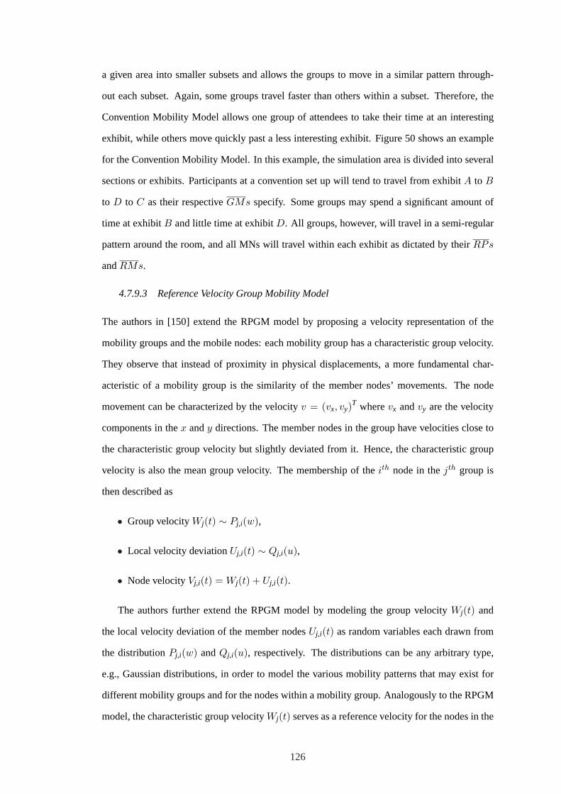
a given area into smaller subsets and allows the groups to move in a similar pattern through-
out each subset. Again, some groups travel faster than others within a subset. Therefore, the
Convention Mobility Model allows one group of attendees to take their time at an interesting
exhibit, while others move quickly past a less interesting exhibit. Figure 50 shows an example
for the Convention Mobility Model. In this example, the simulation area is divided into several
sections or exhibits. Participants at a convention set up will tend to travel from exhibitA to B
to D to C as their respectiveGMs specify. Some groups may spend a significant amount of
time at exhibitB and little time at exhibitD. All groups, however, will travel in a semi-regular
pattern around the room, and all MNs will travel within each exhibit as dictated by theirRPs
andRMs.
4.7.9.3 Reference Velocity Group Mobility Model
The authors in [150] extend the RPGM model by proposing a velocity representation of the
mobility groups and the mobile nodes: each mobility group has a characteristic group velocity.
They observe that instead of proximity in physical displacements, a more fundamental char-
acteristic of a mobility group is the similarity of the member nodes’ movements. The node
movement can be characterized by the velocityv = (vx, vy)T wherevx andvy are the velocity
components in thex andy directions. The member nodes in the group have velocities close to
the characteristic group velocity but slightly deviated from it. Hence, the characteristic group
velocity is also the mean group velocity. The membership of theith node in thejth group is
then described as
• Group velocityWj(t) ∼ Pj,i(w),
• Local velocity deviationUj,i(t) ∼ Qj,i(u),
• Node velocityVj,i(t) = Wj(t) + Uj,i(t).
The authors further extend the RPGM model by modeling the group velocityWj(t) and
the local velocity deviation of the member nodesUj,i(t) as random variables each drawn from
the distributionPj,i(w) andQj,i(u), respectively. The distributions can be any arbitrary type,
e.g., Gaussian distributions, in order to model the various mobility patterns that may exist for
different mobility groups and for the nodes within a mobility group. Analogously to the RPGM
model, the characteristic group velocityWj(t) serves as a reference velocity for the nodes in the
126

group. Therefore, this model is called the Reference Velocity Group Mobility (RVGM) model.
This velocity-based group representation is the time derivative of the displacement-based group
representation in the RPGM model,
Vj,i(t) =dXj,i(t)
dt=
dYj(t)dt
+dZj,i(t)
dt= Wj(t) + Uj,i(t) (80)
In particular, the characteristic group velocityWj(t) is the changes over time inYj(t), the dis-
placement of the group reference center. The reference point representation can be derived from
the reference velocity representation, by integrating the velocitiesWj(t), Uj,i(t), andVj(t) over
an appropriate time interval, given the initial positions of the group reference center and the
mobile nodes.
RVGM model has the following advantages: i) First, it directly provides the mobility pa-
rameters of each mobility group such as its mean group velocity and the variance in the node
velocities within the group; ii) Second, by modeling the node velocities in a mobility group as a
random variable with the distributionQj,i(u), the group membership of any mobile node can be
easily determined, given the nodal velocity and the velocity distributions of the existing mobility
groups.
The velocity representation of RVGM model also provides a clearer characterization of the
mobility groups, as graphically illustrated in Fig. 51 through the transformation of the mobile
nodes from the physical coordinates (Fig. 51a, left box) to the velocity data space (Fig. 51b,
right box). In Fig. 51a, the reference centers of the groups overlap, and the mobile nodes are
scattered with no clear groupings. However, in Fig. 51b, the mobile nodes are concentrated
around the mean group velocity in their respective mobility groups and the mobility groups are
clearly apparent.
127

Figure 51: Mobile Nodes represented by their a) Physical Coordinates, and b) Velocities
128

CHAPTER V
A PROBABILISTIC PREDICTIVE MULTICAST ALGORITHM
IN AD HOC NETWORKS (PPMA)
5.1 Introduction
Ad hoc networks are collections of mobile nodes communicating using wireless media, without
any fixed infrastructure. Conventional multicast routings are inadequate in these scenarios, as
mobility can cause rapid and frequent changes in the network topology. Existing multicast pro-
tocols fall short since node mobility causes conventional multicast trees to rapidly become out-
dated. Frequent state changes require constant updates, reducing the already limited bandwidth
available for data, and possibly never converging to accurately portray the current topology.
Mobility represents the most challenging issue to be addressed by multicast routing protocols.
In fact, if a multicast protocol shows robustness to mobility, it often incurs in other shortcomings
such as protocol overhead or loops. Conversely, if a protocol is primarily designed to limit or to
optimize the network with respect to signaling overhead and power consumption, commonly its
performance degrades with the increase of mobility.
Multicast communications can be classified intosource specificandgroup shared. In source
specificmulticast communication, only one node in the multicast group sends data while all the
other member nodes receive data. Ingroup sharedmulticast communication, each node in the
multicast group wants to send/receive data to/from member nodes. A tree that spans all member
nodes is calledmulticast tree. Multicast trees can be classified intosource rootedandshared
trees, according to the communication strategy. Asource rootedtree has the source node as
root and is optimized for source specific multicast communications. Ashared tree, on the other
hand, is optimized for group shared communications, and connects each group member with all
the other group members.
Tree based multicastis a very well established concept in wired networks, both for source
specific and group shared application support [135]. In the tree based approach, multicast rout-
ing uses a source based or group shared tree among sources and receivers, depending on the
application requirements. This approach is characterized by high bandwidth efficiency, since
129

only one path exists between any pair of nodes. The amount of bandwidth resources required
for building up a tree is commonly less than that required for other multicast delivery structures,
since a multicast tree avoids unnecessary duplication of data [154]. This way, the optimiza-
tion routing problem in tree-based multicast is to find theminimum-weight treethat spans all
the nodes in the multicast group [9][123][147]. However, a multicast tree is more subject to
disruption due to link/node failure and node mobility than more meshed structures.
This chapter explores these contrasting issues, and proposes PPMA, a new Probabilistic
Predictive Multicast Algorithm in ad hoc networks, which leverages the tree delivery structure
for multicasting, solving its drawbacks in terms of lack of robustness and reliability in highly
mobile environments. There is, in fact, a tradeoff between the bandwidth resources used to set up
a multicast tree and the tree robustness to energy node consumption and mobility. The primary
objective of the proposed algorithm is to address this tradeoff, by decoupling tree efficiency from
mobility robustness. The intuition this work is based on is that the deterministic nature which
characterizes traditional multicast protocols tends to become their limiting factor when aiming
at robustness and scalability, especially in highly dynamic ad hoc networks. By exploiting the
non-deterministic nature of ad hoc networks, PPMA takes into account the estimated network
state evolution in terms of node residual energy, link availability, and node mobility forecast,
in order to maximize themulticast tree lifetime. The algorithm statistically tracks the relative
movements among nodes to capture the dynamics in the ad hoc network. PPMA estimates
the nodes’ future relative positions, in order to calculate along lastingmulticast tree. To do
so, it exploits the moststablelinks in the network, while minimizing the total networkenergy
consumption. We propose PPMA in both itscentralizedand distributed version, providing
performance evaluation through extensive simulations.
The remainder of the chapter is organized as follows. In Section 5.2 we review the main
wireless ad hoc network multicast routing protocols which the present work is related to. In
Section 5.3 we describe the motivations and goals of this work, and we introduce our novel
probabilistic cost function. In Section 5.4 we explore the terms our cost function is based on,
and point out their need to reach the described goals. In Section 5.5 we present PPMA, a
Probabilistic Predictive Multicast Algorithm in ad hoc networks, in its centralized version, while
in Section 5.6 the distributed version of the proposed algorithm is described. In Section 5.7 we
show numerical results through extensive simulations run on an ad-hoc simulator. Finally, in
130

Section 5.8 we conclude the chapter.
5.2 Related Work
There have been several multicast routing protocols proposed for wireless ad hoc networks in
literature. In the following we present those which the present work is related to, focusing
on some tree based algorithms which face the problem of determining a robust and reliable
multicast tree in mobile ad hoc networks. We will point out which are their strengths and
weaknesses. In particular, in Sections 5.2.1, 5.2.2, and 5.2.3 we present pros and cons of PAST-
DM (Progressively Adapted Sub-Tree in Dynamic Mesh) [72], ITAMAR (Independent-tree ad
hoc multicast routing) [136], and AODV (Ad Hoc On-Demand Distance Vector Protocol) [132],
respectively. In Section 5.3 we then describe how our proposed probabilistic multicast algorithm
effectively addresses most of their drawbacks.
5.2.1 PAST-DM: Progressively Adapted Sub-Tree in Dynamic Mesh
PAST-DM [72] utilizes avirtual mesh topology, which has the advantage of scaling very well,
since the virtual topology can hide the real network topology regardless of the network dimen-
sion. A multicast session begins with the construction of a virtual mesh connecting all group
members. PAST-DM gradually adapts the virtual mesh to the changes of the underlying net-
work topology in a fully distributed manner [73]. From the computed virtual mesh, a multicast
tree for packet delivery is extracted and then progressively adjusted according to the latest local
topology information. At each node, the topology map is represented as a link state table. The
entry of this table is the link state information of the virtual network, e.g., the hop distance,
which is acquired from the virtual neighbors. Through the link state table, each node has a local
view of the whole virtual topology. In PAST-DM, each source constructs its own multicast data
delivery tree based on its local link state table. In order to minimize the total multicast tree cost,
each source needs to construct a Steiner tree [9], which is extracted from the virtual mesh. To
this end, PAST-DM uses a Source-Based Steiner tree heuristic, which relies on the definitions of
hop distance, cost, andadapted costfor each virtual link. Hop distance is the minimum distance
in terms of number of hops from one of the two nodes of the virtual link to the source node;
costis a generic metric which characterizes the physical link which the virtual link is associate
to; andadapted costof a virtual link is the link cost multiplied by its hop distance to the source.
Thus, for any virtual link which has the source node as one of its two nodes, both its distance
131

value and adapted cost are 0.
PAST-DM computes an approximation of the Steiner tree by exploiting an heuristic, namely
the Source-Based Steiner tree algorithm, which takes the defined adapted costs as key metric to
approximate the Steiner tree. By applying this heuristic, in PAST-DM the source makes all its
neighbors as its children in the multicast tree, and divides the remaining nodes into subgroups.
Each subgroup forms a subtree rooted at one of the first-level children of the source. Then, each
child recursively repeats the Source-Based Steiner tree algorithm. Consequently, the source
node does not need to compute the whole multicast tree; in fact, each child is responsible of
further delivering the data packet to all nodes in its subgroup.
5.2.1.1 Main disadvantages
PAST-DM does not explicitly take into account node mobility prediction in the computation of
the adapted costs, a key metric for the construction of multicast trees. Consequently, weighting
the link cost by a distance that is rapidly changing may result useless, or even incorrect, in a
dynamic environment.
5.2.2 ITAMAR: Independent-Tree Ad hoc MulticAst Routing
ITAMAR [136] finds a set of pre-calculated alternate trees to promptly react to link failures.
This way delay could be reduced whenever a viable backup tree is available at the time of
failure of the current tree. Moreover, backup trees have the advantage of making the tree based
scheme more robust to node mobility. The basic idea of this multicast routing scheme is that
backup multicast trees with minimum number of common links are used to reduce the number
of service interruptions. This improves the mean time between route discoveries, and reduces
the control overhead and the rate of data loss. At the same time, ITAMAR aims to keep the cost
of transmission low. It is worth noting that this method is effective only if the tree failure times
are independent [136]. Thus, under the constraint that nodes move independently, multicast
trees must have no common nodes, and hence no common edges, to be independent. Since
totally independent trees may not be found in many cases, ITAMAR objective is to minimize
the dependence between the failure times, i.e., the correlation of the failure times of the main
tree and the back up tree.
132

5.2.2.1 Main disadvantages
The main disadvantage of ITAMAR [136] is that minimizing the correlation between the main
tree and the back-up tree is a high computational operation, and may not be convenient in all
situations. Also, preventing a link-failure by pre-calculating a tree as much independent from the
previous tree as possible, may result in a greater control messaging overhead, which is required
for route establishment, than that used for repairing only the failed links while leaving all other
tree nodes unchanged. Another disadvantage of ITAMAR is that it does not scale well since it
requires every node to have a global knowledge of the network topology.
5.2.3 AODV: Ad hoc On Demand Distance Vector protocol
AODV [132] routing protocol is capable of unicast, broadcast, and multicast communication.
One of the main advantage of combining in the same protocol unicast and multicast communi-
cation ability is that route information obtained when searching for a multicast route can also
increase unicast routing knowledge, and vice versa. Unicast and multicast routes are discovered
on demand using abroadcast route discoverymechanism. In order to reduce communication
overheads, updates are propagated only along active routes, i.e., routes that have used in the re-
cent past. Broadcast data delivery is provided by using the Source IP Address and Identification
fields of the IP header as a unique identifier of the packet. As nodes join their multicast group, a
multicast tree composed of group members and nodes connecting the group members is created.
A multicast group leader maintains the multicast group sequence number.
5.2.3.1 Main disadvantages
There are some disadvantages in AODV protocol concerning latency, utilization efficiency, mo-
bility robustness, and scalability under particular conditions. As far as latency is concerned,
since routes may differ from the shortest paths, the average data delivery latency is expected to
be higher than in a shortest path algorithm. In terms of resource utilization efficiency, source
routing utilizes a lot of bandwidth due to the use of lists of addresses which increase the size
of the data packet headers. Moreover, since AODV keepshard-statesin its routing table, the
protocol has to actively track and react to changes in the tree. As far as mobility is concerned,
AODV suffers high-rate mobility due to transmission of many routing packets, since each node
maintains a routing table entry for each multicast group for which the node is a member or a
router. Another disadvantage of AODV is that storm of replies and repetitive updates in hosts’
133

caches may occur since nodes make use of their routing caches to reply to route queries. This
leads to poor scalability performance.
5.3 Problem Setup
5.3.1 Motivations and Goals
The main motivations for the introduction of PPMA, a probabilistic predictive algorithm for
multicasting in ad hoc networks, are summarized hereafter:
• The deterministic nature which characterizes traditional multicast protocols tends to be-
come their limiting factor when aiming at robustness and scalability, especially in highly
dynamic ad hoc networks;
• The amount of bandwidth resources required for building up a tree is less than that re-
quired for other more meshed multicast delivery structures;
• The tradeoff between the bandwidth resource required by a multicast tree, and the tree
robustness to energy node consumption and mobility has never been evaluated through
extensive simulations, to the best of the authors’ knowledge.
By exploiting the non-deterministic nature of ad hoc networks, PPMA takes into account the
estimated network state evolution in terms of node residual energy, link availability, and node
mobility forecast, in order to maximize themulticast tree lifetime, and consequently reduce the
number of costly tree reconfigurations. The algorithm statistically tracks the relative movements
among nodes to capture the dynamics in the ad hoc network. This way, PPMA estimates the
nodes’ future relative positions, and computes along lastingmulticast tree. To do so, it exploits
the moststablelinks in the network, while minimizing the total networkenergy consumption.
To achieve these goals, we individuate a set ofgeneral rulesthat aims to achieve such
objectives:
1. The higher battery charge a node avails, the higher its availability to take part in the tree
should be;
2. The higher the number of multicast trees a node belongs to, the lower the node availability
should be;
134

3. If the available battery charge goes under a predetermined thresholdEmin, then a node
should no more be considered available to take part to multicast communications;
4. The larger is the distance between two nodes, the smaller their availability to establish a
communication should be. Obviously, if the distance is larger than a limit rangeDmax, no
link between the nodes should be considered;
5. The more prone a link is to fail or break, the smaller its probability of being included
in a branch of a multicast tree should be. Such a property clearly depends on positions,
speeds, and directions of nodes.
5.3.2 Transmission Energy Model
An accurate model for node energy consumption per bit at the physical layer is in [83][82]
E = Etranselec + βdγ + Erec
elec (81)
where Etranselec is the distance-independent energy utilized by transmitter electronics (PLLs,
VCOs, bias currents, etc.) and digital processing,Erecelec is the energy utilized by receiver elec-
tronics, andβdγ accounts for the radiated power necessary to transmit over a distanced between
source and destination (β andγ are parameters which depend on the environment; the values
considered in this chapter are reported in Tab. 12). As in [112], we assume
Etranselec = Erec
elec = Eelec (82)
Thus, the overall expression forE in (81) simplifies to
E = 2 · Eelec + βdγ (83)
5.3.3 Probabilistic Link Cost
In order to synthesize the properties presented in Subsection 5.3.1, we identify aprobabilistic
link cost function, composed of three multiplicative terms, aEnergy Term, a Distance Term,
and aLifetime Term, which will be extensively explained in Subsections 5.4.1, 5.4.2, and 5.4.3,
respectively. For two generic nodesi andj, we consider as their link costCij the following cost
function
Cij = − log(P Ei · PD
ij · PLij ) (84)
135

where
P Ei = P E
i (Ei , Emini , Emax
i ,Wouti ,Wmax
i ) (85)
is theEnergy Termfor nodei and it weights how much residual energy nodei avails for com-
munications,
PDij = PD
ij (dij , Dmaxi (rreq, εmod
b , ηmodB ), γ) (86)
is theDistance Termbetween nodei and nodej, and it takes into consideration the transmission
power needed by nodei to communicate with nodej, and
PLij = PL
ij (dij , Dmaxi (rreq, εmod
b , ηmodB ), σij ,∆t) (87)
is theLifetime Termbetween nodei and nodej, and it statistically evaluates the probability that
the distance between these two nodes remains bounded for∆t seconds by the maximum trans-
mission range of nodei, Dmaxi , given the current distance. The explanation of the parameters
and variables each term depends on, as well as their units, are reported hereafter for the reader’s
convenience:
Ei [J ] is the battery state of nodei (residual charge);E mini [J ] is the energy threshold under which the
node is no more available, andE maxi [J ] is the node maximum charge;min andmax operators are
extended to all nodes in the network;
Wouti [W ] is the instantaneous power spent for the multicast communications by nodei, andWmax
i [W ]
is the maximum instantaneous power nodei can consume for communications;
dij [m] is the distance between nodei and nodej at time t [s], andDmaxi (rreq, εmod
b , ηmodB ) [m] is the
maximum radio range nodei can reach while guaranteing a bitraterreq [bit/s], given the energy-
per-bitεmodb [J/bit] used in radio transmission, and the spectral efficiencyηmod
B [bit/s/Hz] of the
adopted modulation scheme;
β andγ are parameters which depend on the environment;
∆t [s] is the time interval used for mobility prediction, andσij [m] is the standard deviation of the
gaussian process used in the prediction of the distance evolution between nodesi andj.
All terms are normalized and range in[0, 1] and can be viewed aspseudo-probabilityterms.
Thus, the link cost functionCij in (84) can be viewed as a pseudo-probability. Actually, only the
Lifetime TermPLij is a correctly defined probability, while the other terms are normalized so as to
maintain theCij values in the same variation range. This way, because of the statistical meaning
136

of the link costCij , we can associate a probability metric to the multicast trees computed by
the proposed probabilistic predictive algorithm. TheTree Probabilityis defined as the product
of all the costs of the links included in the tree. This tree probability is obviously expected to
decrease over time, if nodes are not stationary and if their future movements are unknown. The
tree probability can be interpreted as the probability that all the links in a multicast tree will
survive at least for a time period∆t, which is a critical parameter in (87). In Section 5.4 we
describe in detail all the terms of the link cost function in (84), why each of them is necessary,
and their synergic effect to meet the goals outlined in Subsection 5.3.1.
5.4 Probabilistic Link Cost Function Terms
In this Section we describe the properties of each term, which is argument in the link cost
function in (84). In particular, in Section 5.4.1 we detail the Energy Term in (85), in section
5.4.2 we present the Distance Term in (86), and in Section 5.4.3 we derive the Lifetime Term in
(87).
5.4.1 Energy Term
The main purpose of theEnergy Termis to keep all the nodes of the network alive as long as
possible while respecting the general rules 1), 2), and 3), presented in Section 5.3.1. Also, we
want to interpret the Energy Term associated to nodei as the probability of choosing nodei
during the multicast tree construction. So, the Energy Term varies in the range[0, 1] and is a
function of the battery state of the node, i.e., the residual charge. Specifically, it assumes greater
values for those nodes that have a greater residual charge. Hence, givenV the set of indexes
which correspond to the nodes in the network, a first attempt for the Energy Term associated to
nodei could be
Pi(Ei) =( Ei−min n∈VE min
n max n∈VE max
n −min n∈VE minn
)· u(∆min
Ei) (88)
where∆minEi
= Ei −min n∈VEminn and the unit stepu(∆min
Ei) is defined as
u(∆minEi
) =
1 ∆minEi
≥ 0
0 ∆minEi
< 0(89)
Roughly,Pi(Ei) can be viewed as the percentage charge of nodei, with respect to the maxi-
mum possible charge of nodes (max n∈VE maxn ). The reason for the presence ofmin andmax
operators in (88) is that we want to associate to the Energy Term of a node its physical residual
137

0 1 2 3 4 50
0.2
0.4
0.6
0.8
1
battery state [J]
prob
abili
ty
Pi (ε
i )
Pj (ε
j )
εi
max εj
maxε*
Figure 52: Example of thewrongEnergy Term expression in (90)
charge. In fact, if we designedPi(Ei) as the percentage charge of the maximum charge of node
i, we would miss the objective of maximizing the lifetime of all the nodes in the network.
This can be better understood through an example. Figure 52 showsPi(Ei) andPj(Ej) asso-
ciated to nodei and nodej, respectively, according to the following definition for the generic
nodek, where nomin andmax operators are used:
Pk(Ek) =( Ek − E min
k
E maxk − E min
k
)· u(Ek − Emin
k ) (90)
where we choseEmaxi =3 [J ], Emax
j =5 [J ], andEmini = Emin
j = 0 [J ], for sake of clearness. We
note that (90) coincides with the percentage charge of the total charge of the nodek. Also, we
note that nodej has a larger total chargeEmaxj and that, consequentially,Pj(Ej) has a smaller
slope. If nodei and nodej had equal chargeE * , their probabilities in (90) would be different,
sinceEmaxi 6= Emax
j . This way, the charges of the two nodes would not be equally weighted. In
particular, nodei would be more likely to join multicast trees, although equipped with a smaller
energy supply. This simple example evidences the real need formin andmax operators in (88).
Let us point out a drawback in (88): if a new nodeh, equipped with an energy supply
Emaxh higher than any other node in the network, joined the network, we should redefine (88) by
replacingmax n∈VE maxn with Emax
h , where themaxoperator is extended only to the already
138

deployed nodes. Such an obstacle can be avoided either by replacingmax n∈VE maxn with ana-
priori -knownE max, or with a value large enough to hold for most of the nodes in the network. If
the battery charge of nodei becomes lower than itsE mini , such a node cannot join multicast trees
anymore; consequently, the term must be equal to zero. Otherwise, if a node is not currently
involved in any multicast communication, its availability linearly depends on chargeEi . Thus,
all other parameters being equal, we choose the most charged nodes among the possible ones.
Conversely, if a node is involved in some multicast communications, its availability should be
less than the previous case. Moreover, the higher the number of multicast paths a node shares,
the lower its availability should be, according to rule 2) in Section 5.3.1. This behavior can be
ensured by adding an appropriate exponent to (88). Therefore, the finalEnergy Termhas the
following expression
P Ei =
[ Ei −min n∈VE minn
max n∈VE maxn −min n∈VE min
n ] Wmax
iWmax
i −Wouti +ε
u(∆minEi
) (91)
whereε is a positive constant close to 0 whose objective is to avoid a possible division by zero,
and∆minEi
= Ei −min n∈VEminn .
The exponent in (91) is an a-dimensional term, and it increases from 1 to∞ whenWouti
increases from0 toWmaxi . Thus, asWout
i grows toWmaxi , the Energy Term tends to atwo-slope
broken line. More precisely, it has slope equal to zero forEi ∈ [Emini ; Emax
i ), and slope equal to
∞ in Emaxi . In this limit case the term is always equal to zero but inEmax
i .
Figure 53 shows how the Energy Term changes asWouti increases from 0 toWmax
i , where
constants used in (91) can be found in Tab. 12. Since the Energy Term tends to a two-slope
broken line asWouti grows toWmax
i , we can note that the more instantaneous power is spent in
multicast communications by nodei, the less nodei is available to be part of other multicast
communications.
5.4.2 Distance Term
The Distance Term synthesizes the general rule 4) in Section 5.3.1. It takes into account how
much power will be spent by nodei to maintain link(i, j) in the multicast tree. An essential
piece of information to be known is an esteem of the current distancedij (t) between nodei and
nodej, hereon indicated asdij (t). The Distance Term can be expressed as following
PDij =
(Dmax
i − dij (t)Dmax
i
)γ
· u(Dmaxi − dij (t)) (92)
139

0.0010.0635
0.1260.1885
0.2510.3135
0.3760.4385
0.5010 0.2 0.4 0.6 0.8 1 1.2 1.4 1.6 1.8 2
0
0.2
0.4
0.6
0.8
1
Residual charge [J]
Instantaneous power spent [W]
PEi
Figure 53: Energy Term for different values of the instantaneous power spent in multicastcommunications
where
Dmaxi = Dmax
i (rreq, εmodb , ηmod
B ),∀ i ∈ V (93)
Dmaxi is the maximum radio range nodei can reach, and depends on the requested bitrate (rreq),
and on the spectral efficiency (εmodb ) and energy-per-bit (ηmod
B ) characterizing the used modula-
tion scheme, as previously pointed out. In particular, the higher the requested bitrate, the shorter
Dmaxi [68][69].
Clearly, if dij (t) > Dmaxi , the communication link(i, j) does not respect the QoS require-
ments in terms of requested bitraterreq. Thus, in this case,PDij must be 0. As far as the unit
step functionu(.) in (92) is concerned, it is needed to ensurePDij not to be negative for dis-
tancedij (t) greater thanDmaxi . All these considerations explain whyPD
ij decreases from 1 to
0 asdij (t) increases from 0 toDmaxi . In particular, this decrease is characterized by at least a
quadratic trend. In fact, received power decreases over distance with an exponent equal toγ,
according to our propagation model in (83). In free spaceγ is equal to 2, while in a real indoor
or outdoor environment it ranges in the interval [3,5].
140

50 75
100125
150175
200
0 25 50 75 100125150175200
0
0.2
0.4
0.6
0.8
1
Distance between nodes [m]
Max transm
ission range [m]
PDi,j
Figure 54: Distance Term for different transmission ranges
In Fig. 54 the Distance Term for different values ofDmaxi in the range[50, 200] m is de-
picted. It is interesting noting that the larger the maximum radio rangeDmaxi is, the smoother the
decrease of the Distance Term is when the distance between two nodes increases. Conversely,
for low values ofDmaxi , e.g.,50 m, the Distance Term abruptly tends to zero as the distance
between two nodes approaches the maximum radio range. As will be clearer later on, for each
term modeling the link cost in (84), the more graceful the decrease, the slower the degradation
of the link cost itself, and the better the performance achieved by our algorithm.
5.4.3 Lifetime Term
The Lifetime Term synthesizes the general rule 5) in Section 5.3.1. It has a predictive role and
is defined as the probability that the maximum predicted distanced∗ij = MAX Vij (dij (t + ∆t))
between nodei and nodej is smaller or equal thanDmaxi , after∆t seconds elapsed from time in-
stantt. As introduced in (93),Dmaxi is the maximum distance transmitteri can reach. Differently
from [110][111], we consider the following probability
Probd∗ij ≤ Dmaxi |d∗ij = MAX Vij (dij (t + ∆t)) (94)
141

We assumedij (t + ∆t) is a stochastic variable, obtained by summing two other stochastic vari-
ables, namely the distance,dij (t), and the relative velocity between the nodes,Vij , i.e.,
dij (t + ∆t) = dij (t) + Vij (t) ·∆t (95)
The maximum predicted distance ofdij (t + ∆t), d∗ij , is computed in the worst case of node
mobility, i.e., the relative velocity vector lies on the line connecting nodesi and j, and it is
oriented such that the nodes move apart from each other. Hence, we can replace in (95) the
relative velocityVij with its norm|Vij | which we refer to asrelative speed,
d∗ij = dij (t) + |Vij (t)| ·∆t (96)
Consequently, the Lifetime Term is
PLij = Prob(dij (t) + |Vij (t)| ·∆t) ≤ Dmax
i (97)
The determination of this Lifetime Term is a challenging issue, because it generally depends
on several factors. It could be well determined only if the current positions and the future
destinations of nodes were exactly known, as well as their trajectories. Furthermore, a closed-
form expression ofPLij is hard to be found when all possible statistical parameters are taken into
account, even under rough approximations of node mobility. Consequently, some assumptions
about movements of nodes are necessary in order to obtain a useful expression ofPLij . In the
following, we describe the Probability Density Functions (PDFs) ofdij (t) and|Vij |, which are
used to compute the Lifetime Term as in (97).
To determine the PDF ofdij (t), it is worth pointing out that its measured value,dij (t), may
be prone to errors. In most cases, this error can be accurately described by a gaussian PDF
N (dij (t), σdij ), centered atdij (t) and with varianceσ2dij
. Because distances are not negative, we
propose to weight the gaussian PDF by a unit step functionu(y), which is defined in (89), i.e.,
Pdij (t)(y) =1√
2π · σdij
· e− 1
2·(
y−dij (t)
σdij
)2
· u(y) (98)
The varianceσ2dij
can be either set to a fixed value which depends on the measurement system,
as in the case of nodes equipped with Global Position System (GPS) capabilities, or to a value
proportional todij (t), as in the case of nodes capable of measuring relative distances by message
exchanging. Note that (98) is not a well defined PDF, since its integral between−∞ and∞ is
142

−2 −1.5 −1 −0.5 0 0.5 1 1.5 2
−1
−0.5
0
0.5
1
x
erf(x)
Figure 55: erf(x) function
not equal to 1. Thus, we normalize (98) to 1, by means of a functionA(dij (t), σdij ), that is the
area ofPdij (t)(y) over the positive axis multiply by√
2π · σdij . Hence, (98) can be rewritten as
Pdij (t)(y) =1
A(dij (t), σdij )· e− 1
2·(
y−dij (t)
σdij
)2
· u(y) (99)
A(dij (t), σdij ) =∫ ∞
0e− 1
2·(
x−dij (t)
σdij
)2
dx =√
π
2σdij ·
[1 + erf
(dij (t)√2 · σdij
)](100)
where
erf(x) =2√π
∫ x
0e−t2
dt (101)
is depicted in Fig. 55, for sake of clarity.
Figure 56 shows the PDF ofdij (t) as in (99) for different values of the measured distance
between two nodes,dij (t). To derive an expression for the relative speed,|Vij |, some as-
sumptions about node mobility are required. We assume a zero mean gaussian PDF for each
x- and y-component of the velocity vectorVi = Vxi x + Vyiy, characterizing nodei, and
Vj = Vxj x + Vyjy, characterizing nodej. This is equivalent to assuming a Brownian mo-
tion for each node around its current position in the time interval∆t. So, for the generic nodei
we have
PVxiVyi(vxi , vyi
) =1
2π · σ2i
· e− 1
2·(√
v2xi
+v2yi
σi
)2
(102)
whereσ2i is the variance of the conjuncted stochastic processesVxi andVyi
. Consequently, the
amplitude of the velocity vector|Vi | =√
V 2xi
+ V 2yi
which we refer to asspeedof nodei, has a
143

0
20
40
60
020
4060
80100
0
0.01
0.02
0.03
0.04
d i j(t)
[m
]
y [m]
Pd
i j(t)
(y)
Figure 56: PDF as in (99) for different distances between the nodes
Rayleigh PDF,
P|Vi |(x) =x
σ2i
· e−x2
2·σ2i · u(x) (103)
Let us now introduce the relative velocityVij = Vxij x+Vyijy between nodesi andj, whose
x- and y-components are
Vxij = Vxi − Vxj
Vyij= Vyi
− Vyj
(104)
SinceVxi , Vyi, Vxj , andVyj
are gaussian stochastic variables,Vxij andVyijare still gaussian
stochastic variables. Furthermore, by assuming the x- and y-components of the node velocity
vector statistically independent, it results thatVxij andVyijare statistically independent too.
Hence,Vxij has mean equal to the difference of the means ofVxi andVxj , and variance equal to
the sum of the variances ofVxi andVxj . The same holds forVyij. Thus, the conjuncted probability
is
PVxij Vyij(x, y) =
12π · (σ2
i + σ2j )· e− 1
2·√
x2+y2√σ2
i +σ2j
2
(105)
SinceVxij andVyijare zero mean gaussian variables, it results that|Vij | has a Rayleigh PDF.
144
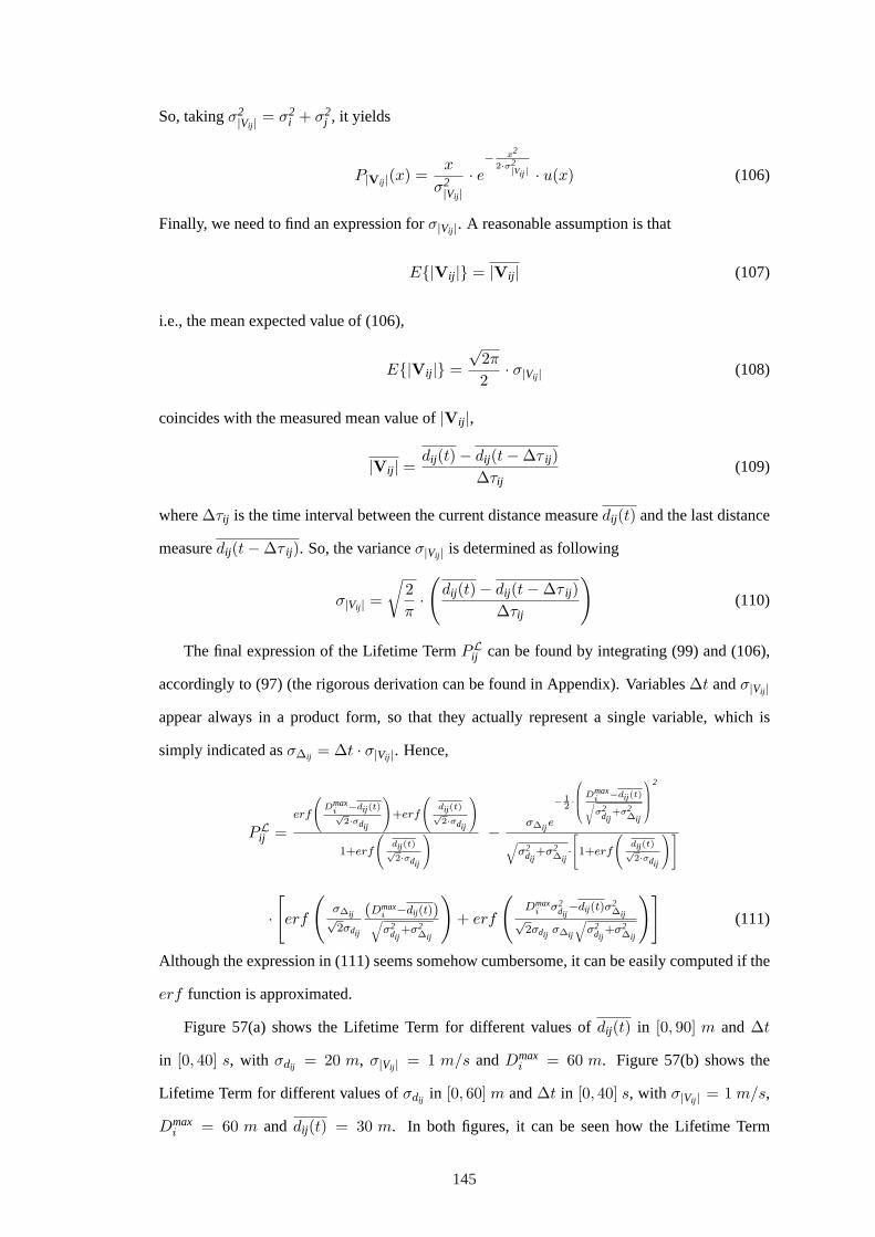
So, takingσ2|Vij | = σ2
i + σ2j , it yields
P|Vij |(x) =x
σ2|Vij |
· e− x2
2·σ2|Vij | · u(x) (106)
Finally, we need to find an expression forσ|Vij |. A reasonable assumption is that
E|Vij | = |Vij | (107)
i.e., the mean expected value of (106),
E|Vij | =√
2π
2· σ|Vij | (108)
coincides with the measured mean value of|Vij |,
|Vij | = dij (t)− dij (t−∆τ ij )∆τij
(109)
where∆τij is the time interval between the current distance measuredij (t) and the last distance
measuredij (t−∆τ ij ). So, the varianceσ|Vij | is determined as following
σ|Vij | =
√2π·(
dij (t)− dij (t−∆τ ij )∆τij
)(110)
The final expression of the Lifetime TermPLij can be found by integrating (99) and (106),
accordingly to (97) (the rigorous derivation can be found in Appendix). Variables∆t andσ|Vij |
appear always in a product form, so that they actually represent a single variable, which is
simply indicated asσ∆ij = ∆t · σ|Vij |. Hence,
PLij =
erf
(Dmax
i −dij (t)√2·σdij
)+erf
(dij (t)√2·σdij
)
1+erf
(dij (t)√2·σdij
) − σ∆ij e
− 12 ·
Dmaxi −dij (t)√σ2
dij+σ2
∆ij
2
√σ2
dij+σ2
∆ij·[1+erf
(dij (t)√2·σdij
)]
·[erf
(σ∆ij√2σdij
(Dmaxi −dij (t))√σ2
dij+σ2
∆ij
)+ erf
(Dmax
i σ2dij−dij (t)σ
2∆ij√
2σdij σ∆ij
√σ2
dij+σ2
∆ij
)](111)
Although the expression in (111) seems somehow cumbersome, it can be easily computed if the
erf function is approximated.
Figure 57(a) shows the Lifetime Term for different values ofdij (t) in [0, 90] m and ∆t
in [0, 40] s, with σdij = 20 m, σ|Vij | = 1 m/s andDmaxi = 60 m. Figure 57(b) shows the
Lifetime Term for different values ofσdij in [0, 60] m and∆t in [0, 40] s, with σ|Vij | = 1 m/s,
Dmaxi = 60 m and dij (t) = 30 m. In both figures, it can be seen how the Lifetime Term
145

decreases as∆t increases. In fact, if the time interval elapsed from the current esteemdij (t) is
large, the mobility prediction based on such esteem may have poor significance. Moreover, it is
worth noting that values of the Lifetime Term close to 1 correspond to low distances between
the nodes, low values ofσdij , and low values of relative speed, i.e., when the nodes are likely to
remain close.
5.5 Centralized PPMA
Algorithm 1 represents the pseudo-code for PPMA, the proposed probabilistic predictive
multicast algorithm, in its centralized version. It extends the centralized Bellman-Ford algorithm
[42], whose objective is to compute the shortest path from the nodex to the sources, with
respect to a certain metric, for every nodex in the network. The centralized Bellman-Ford
algorithm builds up a spanning tree which hass as its root. It chooses the fatherfx of a nodex
by minimizing the cost of the associated path towards. The multicast tree connecting the source
node with the receiver nodes is extracted from the computed spanning tree. This procedure leads
in general to several unicast paths, which inefficiently connect the sender to the receivers with
no bandwidth saving. On the other hand, the spanning tree has the good property that it does
not distinguish the receiver nodes from the other nodes. This property can be fruitfully used if
some nodes want to become a receiver, since a path from the new member node to the senders
has already been computed.
Centralized PPMA, our centralized solution for the computation and set up of multicast
trees, differs from the centralized Bellman-Ford in the crucial choice of a node predecessor.
There are a number of ways to choose the father of a node in order to create a multicast tree.
In the following, we propose two different criteria applied by centralized PPMA to efficiently
address this issue, namely theDistance-basedcriterion and theLink Cost-basedcriterion.
As can be seen in the initialization phase of Algorithm 1, namely‘INIT’ , we define some
useful node sets in order to explain how PPMA works. LetV be the set of all the nodes of the
network, andM the set of all the multicast groups. For a given multicast groupm ∈ M, and
a given maximum number of hops, the current nodex will choose a predecessor in its set of
potential predecessorsPP(x). We consider a generic nodev ∈ V a potential predecessor of
146

0
30
60
90
0
10
20
30
40
0
0.2
0.4
0.6
0.8
1
d i j(t) [m
]∆(t) [s]
PLi j
(a)
0
20
40
60
010
2030
40
0
0.2
0.4
0.6
0.8
1
σ d i j
[m]
∆(t) [s]
PLi j
(b)
Figure 57: Lifetime Term for different transmission ranges (Fig. 57(a)), and for differentvalues ofσij (Fig. 57(b))
147

Algorithm 1 Centralized PPMA
INIT :1: nodes set of the network→V2: multicast groups set→M3: ∀m ∈M :4: source→ s5: current node → x6: father of x→ fx
7: cost of link (i, j)→ Cij
8: path from x to s→ Px
9: cost of path from x to s→ CPx
10: H(x) ≡ h ∈ V | fh = xchild set11: N (x) ≡ n ∈ V | Cnx < ∞neighbor set12: A(x) ≡ a ∈ V | dsa < dsxpositive advance set13: W ≡ w ∈ V | ∃ Pw, CPw < ∞set of nodes with a feasible path to s14: F ≡ f ∈ V | H(f) 6≡ ∅set of nodes with at least a child15: PP(x) ≡ N (x) ∩ A(x) ∩Wpotential predecessor set16: PF(x) ≡ PP(x) ∩ Fpredecessor father set
CENTRALIZED PPMA:1: for all m ∈M do2: for all number of hops do3: for all x ∈ V do4: for all i ∈ V −H(x) do5: FIND SET(PP(x))6: FIND SET(PF(x))7: PF in(x) ← (K(x) ∩ PF(x))8: if PF in(x) ≡ ∅ then9: PFout(x) ← (PF(x)− PF in(x)
)10: if PFout(x) ≡ ∅ then11: NF(x) ← (PP(x)− PF(x))12: if NF(x) ≡ ∅ then13: fx ← NULL
14: elseNF(x) 6≡ ∅15: fx ← ARGMINj
(CPj + Cjx
), ∀j ∈ NF(x)
16: end if17: elsePFout(x) 6≡ ∅18: fx ← FIND FATHER OUT (PFout(x))19: end if20: elsePF in(x) 6≡ ∅21: fx ← FIND FATHER IN
(PF in(x))
22: end if23: end for24: end for25: end for26: end for
148

Algorithm 2 Choice of predecessor
INIT :1: current radio transmitting range of node k → Dk
TX
DISTANCE-BASED CRITERION:1: K(x) ≡ k ∈ V | dkx ≤ Dk
TX2: FIND FATHER OUT ← ARGMINz (dzx −Dz
TX) , ∀z ∈ PFout(x)3: FIND FATHER IN ← ARGMINw (dwx −Dw
TX) , ∀w ∈ PF in(x)
L INK COST-BASED CRITERION:1: K(x) ≡ k ∈ V | Ckx ≤ Ckhmax, hmax = ARGMAX h(Ckh), h ∈ H(k)2: FIND FATHER OUT ← ARGMINz (Czx− Czhmax) , hmax = ARGMAX h(Czh), h ∈H(z), ∀z ∈ PFout(x)
3: FIND FATHER IN ← ARGMINw (Cwx− Cwhmax) , hmax = ARGMAX h(Cwh), h ∈H(w), ∀w ∈ PF in(x)
nodex, if nodev belongs to the intersection of the three sets defined below
N (x) = n ∈ V | Cnx < ∞ neighbor set
A(x) = a ∈ V | dsa < dsx positive advance
W = w ∈ V | ∃ Pw, CPw < ∞ nodeswith a path to s
(112)
whereCij is the cost of link(i, j), according to (84);dxy is the distance between nodex and
nodey; Px is a feasible path from nodex to the senders; CPx is the cost of the pathPx, i.e., the
sum of the cost of the links that belong toPx, formally defined as
CPx =∑
(i,j)∈Px
Cij (113)
We can define the set of potential predecessor of nodex, PP(x), as
PP(x) = N (x) ∩ A(x) ∩W (114)
The setN (x) contains all the neighbors of nodex, and imposes that the predecessor ofx has to
be necessarily a neighbor ofx, where a noden is defined as a neighbor ofx if the cost of the link
(n, x) is lower than∞, i.e.,Cnx < ∞. Note that, according to (84) and (92), the link cost may
be∞ if the distance between the two nodesn andx exceeds the maximum radio transmitting
range of noden. The setA(x) is the positive advance set, and contains all the nodes located
inside the circle of radiusdsx arounds. The setA(x) is needed in (114) in order to avoid loop
formation during the construction of the tree, as proved in [112]. The last set in (114),W,
contains all the nodes that know a feasible path towardss. A potential predecessorw of x must
know a feasible path toward the senders, otherwise nodex cannot receive any packet froms.
149

The setPP(x) can be further partitioned in two subsets:PF(x), i.e., the set ofpredecessor
fathernodes, andNF(x), i.e., the set ofpredecessor not-fathernodes. It holds that
PP(x) ≡ PF(x) ∪NF(x), PF(x) ∩NF(x) ≡ ∅ (115)
1) The first subset,PF(x), is composed of those potential predecessors that currently have
other children, so we can call them potential predecessor fathers, where thechild setof nodea
is defined as the set of nodes whose father isa. Hence,
H(a) ≡ h ∈ V | fh = a (116)
We can define a generalfather setF as
F ≡ f ∈ V | H(f) 6≡ ∅ (nodeswith at least one child) (117)
which all the network nodes that have at least one child belong to. Thus, the predecessor father
set can be expressed as
PF(x) ≡ PP(x) ∩ F (118)
2) The second subset,NF(x), is composed of the remaining potential predecessors and can
simply be defined as
NF(x) ≡ PP(x)−PF(x) (119)
In Fig. 58 a simple example of partition ofPP(x) is depicted. If a link between two nodes is
available, i.e., the link cost is lower than∞, it is depicted with a solid arrow, while the multicast
tree is depicted with dashed arrows. Nodex, the current node, has to choose its predecessor.
The potential predecessors set ofx, PP(x), is composed of nodesb, c andd. It is easy to verify
that all these nodes belong to the setsA(x), N (x) andW. In fact, they belong toN (x) since
they are neighbors ofx. Moreover, they belong toA(x) since their distance towards is less than
the distance froms to x. Finally, they belong toW, since they all have joined the multicast tree,
and thus know a feasible path toward the senders. However, as can be seen in Fig. 58, only
nodesb andc have not a void child set. In fact, the child set of nodeb, H(b), is composed of
two nodes, nameless in the figure, and the child set of nodec,H(c), contains noded. Thus, the
potential predecessor father set ofx, PF(x), is composed of nodesb andc, while the not-father
set,NF(x), coincides with noded.
In the choice of the predecessorfx of x, Centralized PPMA gives higher priority to the
elements ofPF(x) than to the elements ofNF(x). PPMA tries to avoid building up a multicast
150

PP(x)
s
x
d
a
b
c
H(b)
H(c)
PF(x)
Multicast tree
Link
PP(x)
s
x
d
a
b
c
H(b)
H(c)
PF(x)
Multicast tree
Link
PP(x)
s
x
d
a
b
c
H(b)
H(c)
PF(x)
PP(x)
s
x
d
a
b
c
H(b)
H(c)
PF(x)
Multicast tree
Link
Multicast tree
Link
Figure 58: Centralized PPMA: partition of the potential predecessor setPP(x)
tree composed of unicast paths, by giving higher priority to those nodes that match a predefined
requisite, e.g., being a father. Although such a process could lead to a high tree cost, the total
number of links of the spanning tree is kept low. The rationale of this strategy is to exploit
those links that are already used to reach some other receivers. In fact, this is the key feature of
multicasting. Hence, PPMA prefers father nodes, and connects nodex to s, when it is possible,
by exploiting already used paths.
The setPF(x) is divided in two other subsets,PF in(x) andPFout(x), which will be given
different priorities in the choice of the predecessor of nodex, as will be clearer in the following.
So we have,
PF(x) ≡ PF in(x) ∪ PFout(x), PF in(x) ∩ PFout(x) ≡ ∅ (120)
In particular, PPMA prefers to choose the nodes that belong toPF in(x) as predecessor of node
x than the nodes that belong toPFout(x). We propose two different‘criteria’ to partition the set
PF(x), the‘Distance-based’criterion and the‘Link Cost-based’criterion, which are described
in details in the following subsections.
151

5.5.1 Distance-Based Criterion
The first criterion, namely the‘distance-based’criterion, distinguishes the elements ofPF(x)
that have a current radio transmitting rangeDTX large enough to reach nodex, from those that
have not. Thus, according to such criterion, the setPF in(x) ⊆ PF(x) contains the nodesf in
that are transmitting to some other nodea which is located at a distancedf ina from f in larger
than the distancedf inx betweenf in andx. We can formally definePF in(x) as
PF in(x) ≡ f in ∈ PF(x) | df inx ≤ Df in
TX (121)
whereDf in
TX is the current radio transmitting range of nodef in. Differently, a node that has to
increase its current radio transmitting range to allow nodex to receive the packets it sends, is
included inPFout(x). So
PFout(x) ≡ fout ∈ PF(x) | dfoutx > Df out
TX (122)
Figure 59(a) shows an example of network topology that explains this concept. A source
s and three receivers,r1, r2, andr3, must be connected by a multicast tree. The multicast
tree is depicted with unidirectional dashed arrows, while unidirectional solid arrows are used
to represent existing links (whose costs are shown nearby), and bidirectional dotted arrows
indicate distances. Receiversr1 andr3 have joined the tree through nodesb andc, respectively,
but receiverr2 has not joined the tree yet. Since both nodesb andc have a child, thepotential
predecessor setand thepredecessor father setof receiverr2 coincide, and are composed of
nodesb andc, so thatPP(r2) ≡ PF(r2) ≡ b, c. However, the current radio transmitting
range of nodeb, DbTX, is larger than the distancedbr2 from b andr2, while the radio transmitting
range of nodec, DcTX, is smaller thandcr2. Thus,
PF in(x) ≡ b, PFout(x) ≡ c (123)
Thus, receiverr2 is connected to the senders through the predecessorb, which does not have
to increase its current radio transmitting range to reachr2. Note that, according to this partition
criterion, the costs of the links(c, r2) and(b, r2) have not influence in the partition ofPF(r2),
i.e., in the priority given to the nodes.
152

d(b,r2)
DTXb
DTXc
d(c,r2)
r1
s
r3
a
c
3
1
1
1 1
Radio TX range
Distance
Multicast tree
Link
b r2d(b,r2)
DTXb
DTXc
d(c,r2)
r1
s
r3
a
c
3
1
1
1 1
Radio TX range
Distance
Multicast tree
Link
b r2d(b,r2)d(b,r2)
DTXbDTXb
DTXcDTXc
d(c,r2)d(c,r2)
r1
s
r3
a
c
3
1
1
1 1
Radio TX range
Distance
Multicast tree
Link
b
r1
s
r3
a
c
3
1
1
1 1
Radio TX range
Distance
Multicast tree
Link
Radio TX range
Distance
Multicast tree
Link
Radio TX range
Distance
Multicast tree
Link
b r2
(a)
r1
s
r2
r3
a
b
c
1
31
1
1
3
1
Multicast tree
Link
r1
s
r2
r3
a
b
c
1
31
1
1
3
1
Multicast tree
Link
r1
s
r2
r3
a
b
c
1
31
1
1
3
1
r1
s
r2
r3
a
b
c
1
31
1
1
3
1
Multicast tree
Link
Multicast tree
Link
(b)
Figure 59: Centralized PPMA: partition ofPF(x) in PF in(x) andPFout(x) based on the‘distance’criterion (Fig. 59(a)), and based on the‘link cost’ criterion (Fig. 59(b))
153

5.5.2 Link Cost-Based Criterion
The second proposed criterion for partitioning the predecessor father setPF(x), namely the
‘link cost-based’criterion, considers link costs instead of distances. In this case,PF in(x) con-
tains the nodesf in ∈ PF(x) such that the maximum cost of the links towards their children,
Cf inhmax is greater thanCf inx, wherehmax is the child off in which corresponds to the maximum
cost of the link fromf in. That is,
PF in(x) ≡ f in ∈ PF(x) | Cf inx ≤ Cf inhmax (124)
hmax = ARGMAX h(Cf inh), h ∈ H(f in)
Differently, if a nodef out does not connect a childh, whose associated link costCf outh is greater
thanCf outx, thenfout is included inPFout(x). That is,
PFout(x) ≡ fout ∈ PF(x) | Cf outx > Cf outhmax (125)
hmax = ARGMAX h(Cf outh), h ∈ H(fout)
It is worth pointing out that, if we choose the distancedij between nodei and nodej as
the metric to compute the cost of the link(i, j), the ‘distance-based’criterion and the‘link
cost-based’criterion coincide. Anyway, this second criterion can be viewed in general as an
extension of the first one, since the link cost could account for the node speed or the battery
charge in addition to the distance.
To illustrate this second criterion, Fig. 59(b) shows the same network topology depicted in
Fig. 59(a), but with different link costs. Let us assume that the metric of the link cost takes
also into account therelative speedof the nodes, i.e., the higher the relative speed between two
nodes, the higher the cost of the link connecting them. As in the previous example, in Fig. 59(b)
sources and three receivers,r1, r2, andr3, must be connected by a multicast tree, wherer1 and
r3 have joined the tree through nodesb andc, respectively, whiler2 has not joined the tree yet.
Since both nodesb andc have a child, the potential predecessor set and the predecessor father
set of receiverr2 coincide, and are composed by nodesb andc,
PP(r2) ≡ PF(r2) ≡ b, c (126)
However, the cost of the link(b, r1) is smaller than the cost of the link(b, r2), while the cost of
the link (c, r3) is larger than the cost of the link(c, r2). Thus,
PF in(x) ≡ c, PFout(x) ≡ b (127)
154

Note that, according to this partition criterion, the distancesdcr2 anddbr2 have influence in the
partition ofPF(r2), i.e., in the priority given to the nodes, since the distance between nodes is
included in the computation of the link cost. Thus, the receiverr2 is connected to the senders
through the predecessorc, which is already connecting a child through a link with a higher cost
thanCcr2.
In general, the partition of the setPF(x) can be obtained by intersecting it with another set,
K(x), that depends on the used kind of partition.
1) In the case of the‘Distance-based’partition, the setK(x) is defined as
K(x) ≡ k ∈ V | dkx ≤ DkTX (128)
2) whereas, in the case of the‘Link Cost-based’partition, the setK(x) is defined as
K(x) ≡ k ∈ V | Ckx ≤ Ckhmax (129)
hmax = ARGMAX h(Ckh), h ∈ H(k)
Once the setK(x) is defined, the setsPF in(x) andPFout(x) are easily obtained as:
PF in(x) ≡ PF(x) ∩ K(x) (130)
PFout(x) ≡ PF(x)− PF in(x) (131)
So far, we defined three sets,PF in(x), PFout(x) andNF(x), which contain all the pos-
sible predecessors for the current nodex. As explained in Algorithm 1, PPMA looks for the
predecessor ofx, fx, primarily in thePF in(x) set. Then, if that set is void, PPMA searchesfx
in thePFout(x) set, and finally, if alsoPFout(x) is void, in theNF(x) set. However, we did
not explain how PPMA chooses the predecessor ofx, among the elements of each set. To this
end, we propose three criteria of choosingfx in a given setP(x).
1) The first one chooses the nodefx such that the path from the receiverx to the senders
has the minimum cost, i.e.,
fx ← ARGMINj
(CPj + Cj,x
),∀j ∈ P(x) (132)
2) The second one chooses the nodefx such that the link from it to the receiverx has the
minimum link cost, i.e.,
fx ← ARGMINj (Cjx) , ∀j ∈ P(x) (133)
155

3) The third and last one takes into account the differences between the distances or between
the link costs, whether the partition of the setP(x) is ‘Distance’-based or ‘Link Cost’-based,
respectively. In the former case, the difference is between the current radio transmitting range
of the node candidate as predecessor ofx and the distance withx, i.e.,
fx ← ARGMINz (dzx −DzTX) ,∀z ∈ P(x) (134)
In the latter case, the difference is between the cost of the link between the candidate andx and
the maximum cost of the link between the candidate and its children, i.e.,
fx ← ARGMINz (Czx− Czhmax) (135)
hmax = ARGMAX h(Czh), h ∈ H(z), ∀z ∈ P(x)
Each of the above three criteria can be used by two functions, ‘FIND FATHER IN ’ and
‘ FIND FATHER OUT’, to choosefx in the setsPF in(x) andPFout(x), respectively. The choice
among the elements ofNF(x), instead, is always based on the first criterion, as in (132).
To summarize, as described in Algorithm 1, if the setPF in(x) is not void, Centralized
PPMA chooses the predecessor ofx, fx, in that set, using the function ‘FIND FATHER IN ’.
Otherwise, if the setPF in(x) is void, PPMA finds the setPFout(x), and, if the set is not void,
the predecessor ofx is chosen by the function ‘FIND FATHER OUT’. If also this set is void,
fx is chosen among the elements that belong toNF(x), according to the criterion in (132). In
Algorithm 2 we propose two algorithms, theDistance-basedand theLink Cost-basedalgorithm,
based on the criteria described in (134) and (135), respectively. Each algorithm defines the set
K(x) in order to partitionPF(x), and also defines the two functions ‘FIND FATHER IN ’ and
‘ FIND FATHER OUT’ to choosefx among the elements ofPF in(x) andPFout(x), respectively.
5.6 Distributed PPMA
Algorithm 3 represents the pseudo-code for Distributed PPMA, the proposed probabilistic pre-
dictive multicast algorithm in its distributed version. In order to build up a multicast tree, Dis-
tributed PPMA uses two different types of link costs: aprivate link cost, denoted withCpriv,
and apublic link cost, denoted withCpub. Theprivate link costis used by all nodes, except the
receivers not already connected to the tree, to find a minimum cost path toward the source. The
public link costis used by the receivers not already connected to the tree to aggregate the paths,
156

which have been computed using the private costs, to form multicast trees. This way, i) the
number of nodes that belong to the tree is reduced, and ii) the overhead for control messages is
kept low.
For each link we have oneprivate link cost, and as manypublic link costsas the total number
of multicast groups. The private link costs are computed as in (84), whereas the public link costs
either coincide with the private link costs, if the link is not used in a multicast tree, or are set to
0, if the link is part of a multicast tree. The terms‘public’ and‘private’ account for the fact that
the two types of costs are or are not ‘visible’ to the not already connected receivers, respectively.
LetM be the set of the multicast groups for a given multicast groupm ∈M.
If a nodex is a receiver (x ∈ Rm), it may or may not have just joined the tree.
If the receiver has joined the tree (x ∈ T m), it tries to find a new paths,Pnew, which respects
thepositive advanceand whose private cost,CPprivmin
priv , is lower than the private cost of the current
path,CPcurrentpriv . If a lower cost path is found, the receiver changes path only ifnew cost <
current cost. This condition ensures that the path change is convenient, i.e., the new path has
a sufficiently lower cost than the current one so that resources spent for changing path will be
repaid by the saving induced by the new path, as will be explained in the following. If this
condition holds, theSWITCH FATHER function switches the old predecessor of nodex, fPcurrentx ,
with the new one,fPnewx . Then, theUPDATE CURRENT COSTS function changes the public
link cost ofPcurrent links with their private costs, and theUPDATE NEW COSTSfunction sets
the private link costs ofPnew links to 0.
If a receiver has not joined the tree (x 6∈ T m), Distributed PPMA finds the pathP∗ with
minimum public cost, i.e.,ARGMINP (CPpub). The public cost of a path is computed by summing
all the public costs of the links which are part of the path. If such a path is found, the receiver
joins the tree and sends to its new father,fP∗x , a JOIN message to establish the link. Finally, it
sets to 0 the public costs of thePcurrent links.
If a node is not a receiver (x 6∈ Rm), it finds the most convenient path between the available
public pathsandprivate paths, and stores the related father. Whenever another node asks for
the cost of the path to the source, the node will give these pieces of information.
Figure 60 shows how thenew cost and thecurrent cost are computed by Distributed
PPMA. For sake of clarity a simple network topology has been chosen. The values of theprivate
costsare shown nearby the link arrows. A receiverx is currently connected to the source via
157

Algorithm 3 Distributed PPMA
INIT :1: nodes set of the network→V2: multicast groups set→M3: set of receivers→Rm, ∀m ∈M4: multicast tree → T m
5: current node → x6: path→ P ∈ T m path from x to sm7: private cost of path P → CPpriv
8: public cost of path P → CPpub
9: father of x via P → fPx10: H(x) ≡ h∈V | ∃ P ∈ T , fPh ≡ x child set
DISTRIBUTED PPMA:1: for all m ∈M do2: if (x ∈ Rm) then3: if (x ∈ T m) then4: Pnew← ARGMINPpriv
min ,Pcurrent(Cpriv)
5: if Pnew 6= NULL then6: NEW& CURRENT COSTS(Pnew,Pcurrent)7: if (new cost < current cost) then8: SWITCH FATHER(fPcurrent
x , fPnewx )
9: UPDATE CURRENT COSTS(Pcurrent)10: UPDATE NEW COSTS(Pnew)11: end if12: end if13: elsex 6∈ T m14: P∗ ← ARGMINP (CPpub))15: JOIN(fP∗x )16: UPDATE NEW COSTS(P∗)17: end if18: elsex 6∈ Rm19: Ppriv
min ← ARGMINP(CPpriv)20: Ppub
min ← ARGMINP(CPpub)21: P+← ARGMINPpriv
min ,Ppubmin
(Cpriv, Cpub))22: if P+ 6= NULL then23: STORE(P+ , CP+
priv, CP+
pub)24: end if25: end if26: end for Daemon running ∀x ∈ V
158

NEW& CURRENT COSTS:1: fx ← fPcurrent
x
2: max1 ← MAX y(Cxy), ∀ y ∈ H(x) ∩Rm
3: max2 ← MAX (max1, Cxf x)
4: max3 ← MAX z(Cf xz),∀ z ∈ H(fx) ∩Rm− x5: max4 ← MAX w(Cf xw),∀ w ∈ H(fx) ∩Rm
6: new cost ← CPnewpriv + max2 + max3
7: current cost ← CPcurrentpriv − Cf xx + max1 + max4
New path cost
Current path cost
Multicast tree
Link
r2
s
x
r7
a
b
c
1
314
1
1 3
r3
r11
2
r8
1
r64
r4
r51
2
New path cost
Current path cost
Multicast tree
Link
r2
s
x
r7
a
b
c
1
314
1
1 3
r3
r11
2
r8
1
r64
r4
r51
2
New path cost
Current path cost
Multicast tree
Link
New path cost
Current path cost
Multicast tree
Link
New path cost
Current path cost
Multicast tree
Link
r2
s
x
r7
a
b
c
1
314
1
1 3
r3
r11
2
r8
1
r64
r4
r51
2
r2
s
x
r7
a
b
c
1
314
1
1 3
r3
r11
2
r8
1
r64
r4
r51
2
Figure 60: Distributed PPMA: computation ofcurrent cost andnew cost as in Algorithm 3
159

nodec, so thatPcurrent = x c a s is the current path fromx towards the senders. Let us assume
thatx finds another path towardss, Pnew = x b a s, which has a lower private cost thanPcurrent,
i.e.,CPnewpriv < CPcurrent
priv . In Fig. 60, we can see that this condition holds, since
CPcurrentpriv = Csa + Cac + Ccx = 1 + 4 + 3 = 8 < 3 =
= 1 + 1 + 1 = Csa + Cab + Cbx = CPnewpriv (136)
In such a situation, nodex has to check ifnew cost < current cost. As can be seen in the
‘ COMPUTE COSTS’ subroutine of Algorithm 3,current cost is composed of four terms,
current cost ← CPcurrentpriv − Cf xx + max1 + max4 (137)
The first term,CPcurrentpriv , is the cost of the current path froms to x. The second term,Cf xx, is the
cost of the link(fx, x). The third term,max1, is the highest private cost of the links betweenx
and its receiver children, i.e.,
max1 ← MAX y(Cxy), ∀ y ∈ H(x) ∩Rm (138)
H(x) ≡ h ∈ V | fh = x, fh predecessor of node h
The fourth term,max4, is the highest cost of the links betweenfx and its children, for all the
children offx, as shown below,
max4 ← MAX w(Cf xw), ∀ w ∈ H(fx) ∩Rm (139)
The sum of these four terms is thecurrent cost and represents the cost of the sub-tree that
connects the source to nodex, and nodex to i) its receiver child, which is associated to the
highest private link cost, and ii) the receiver child offx, which is associated to the highest private
link cost, exceptx. Note that Distributed PPMA accounts for the communication broadcast
nature in ad hoc networks, since it computes the cost of the sub-tree by summing, for each node
belonging to such subtree, only the highest private link cost among all the outgoing links.
In Fig. 60, the cost of the link(fx, x), i.e.,(c, x), is3 and only the receiversr4 andr5 belong
to H(x). So,max1 is Cxr5, since the cost of the link(x, r4) is lower than the cost of the link
(x, r5) (Cxr4 = 1 < 2 = Cxr5). Moreover,max4 is Ccr6 = 4, since receiverr6 is the child of
nodec associated to the highest link cost.
If nodex changes its predecessor, it must be ensured that the new path has not a higher cost
than the current one. However, we cannot know this, since we should know which links belong
160

to both the new and the current paths. Thus, we need aworst-case formulathat guarantees a
convenience for the change of the predecessor. To this end,new cost is defined as
new cost ← CPnewpriv + max2 + max3 (140)
where the first term,CPnewpriv , is the cost of the new path found by nodex. The second term,max2,
is the maximum betweenmax1 and the cost of the link connectingx to its current predecessor
fx, i.e.,
max2 ← MAX (max1, Cxf x) (141)
Finally, the third term,max3, is the highest cost of the links betweenfx and its receiver children,
exceptx, i.e.,
max3 ← MAX z(Cf xz), ∀ z ∈ H(f) ∩Rm− x (142)
Hence,new cost represents the cost of the possible sub-tree connecting the nodes we described
in the interpretation ofcurrent cost. In fact, it may be necessary to reroute the children of the
current predecessor ofx onto the new path found byx.
In the case shown in Fig. 60,max2 is equal to3 since the cost of the link betweenx and
its predecessorfx = c, Cxc, is higher thanmax1. In the figure we considered bidirectional
links, where the link cost is the same in both directions, for sake of simplicity. With this as-
sumption,max3 coincides withmax4. The links involved in the computation ofnew cost and
current cost are shown in figure with a dotted and dash-dotted lines, respectively. Finally, we
can compute them as in the following,
current cost = Csa + Cac + Ccr6 + Cxr5 = 1 + 4 + 4 + 2 = 11
new cost = Csa + Cab + Cbx + Cxc + Ccr6 = 1 + 1 + 1 + 3 + 4 = 10
According to this example, nodex will change its predecessor sincenew cost is smaller than
current cost.
5.7 Performance Evaluation
This section deals with the performance evaluation of our developed algorithms. In particular,
in Subsection 5.7.1 we review the most commonly used mobility models for ad hoc networks
in the literature, and describe the mobility model which has been developed and used in this
chapter. Then, in Subsection 5.7.2 we describe the simulation scenario, and present the main
achieved results.
161

5.7.1 Network Mobility Model
The network of nodes is represented as(V, D), whereV = v1, .., vN is a finite set of nodes
in a finite-dimension terrain, withN = |V|, andD is a matrix whose element(i, j) contains the
value of the distance between nodesvi andvj . As far as the mobility models in ad hoc networks
are concerned, the most commonly used models will be briefly described hereafter. Then, we
propose our mobility model which is an extension to the Random Walk Model (RWM).
5.7.1.1 Random WayPoint Model (RWPM)
In this model, nodes in a largeroomchoose some destination, and move there at a random speed
uniformly chosen in(0;Vmax]. Once a node has reached its destination point, it pauses for a
timeP [s] uniformly chosen in[0, Pmax]. If the terrain border effectsare modeled considering
a wrap around1 environment, in the steady state a uniform distribution of nodes in the whole
region is generated, whereas if abounced back2 is considered, a lower node density in proximity
of the borders can be noticed.
5.7.1.2 Random Walk Model (RWM)
This model has been proposed by Einstein in 1926 to mimic particle’s Brownian movement.
A node starts moving by picking up a random direction uniformly in[0, 2π]. It continues the
movement for a certain time, and then repeats the direction selection again. If during this period
it hits the region border, different policies can be implemented to take into account the border
effect. The node, in fact, can either bebounced back, or continue its movement as if it were in
a wrap aroundenvironment, or bedeleted and replaced3 by another node which is placed in a
random position inside the region. The first two solutions are in this model equivalent, giving
both a uniform distribution of nodes in the steady state, while the latter solution concentrates
nodes in the center of the region. The choice of speed is the same as in the Random WayPoint
Model.
1In a wrap aroundenvironment, nodes are assumed to seamlessly move from a side of the terrain to its oppositeside, as if the two sides coincided, i.e., all the boundaries of the terrain are assumed to be melted together.
2In a bounced backenvironment, nodes are assumed to bounce when approaching one side of the terrain, as a“ball bounces against a wall”.
3In a deleted and replacedenvironment, nodes approaching a side of the terrain are virtually ‘deleted’ and ‘re-placed’ by another node, which is placed inside the terrain according to a pre-established rule.
162

Table 11: Network node mobility
Mobility 4 Vmax[m/s] Amin[m/s2] Amax[m/s2]Low 5 −3 2
Medium 10 −5 3High 15 −7 5
5.7.1.3 Random Direction Model (RDM)
This model is similar to theRandom WalkModel, differing from that only as far as the node
behavior in the border of the region is concerned. In this model a node hitting the border will
choose its next direction towards the inside half plane. The angle formed by the node direction
and the tangent line of the border is chosen uniformly in[0, π].
5.7.1.4 Extended-Random Walk Model (E-RWM)
In this chapter we extend theRandom Walkmodel to include accelerations and decelerations,
the main difference being that the speed of a node can change according to an instantaneous
acceleration and deceleration, as shown in the following formula which uses parameters in Tab.
11.
v(t + ∆tmob) = max(Vmin,min(v(t) + a ·∆tmob, Vmax)) (143)
a ∈ [Amin, 0], pa > 0.5
a ∈ [0, Amax], pa ≤ 0.5;(144)
x(t + ∆tmob) = x(t) + v(t + ∆tmob) · cos(φ)
y(t + ∆tmob) = y(t) + v(t + ∆tmob) · sin(φ)(145)
wherepa andφ are stochastic variables uniformly distributed in[0, 1] and[0, 2π], respectively.
In (143) the node velocityv(t) can change every∆tmob [s], under the constraint thatVmin ≤v(t) ≤ Vmax, and the additional constraint that its derivativea [m
s2 ], the node acceleration, is
bounded, i.e.,Amin ≤ a ≤ Amax.
Moreover, in the performed simulation nodes belonging to the same multicast group are
grouped into a cluster, which is modeled as a set of nodes deployed in a circular area with a
given radius. The source of the relative multicast groups is in the center of this area. Inside
a cluster, all nodes move with a low relative speed with respect to the source, i.e., nodes in a
4Velocity is uniformly distributed withVmin = 0 for each scenario.
163

Table 12: Simulation parameters
Parameter ValueEelec 5 [nJ/bit]
β 100 [pJ/bit ·mγ ]γ 3
[Emin, Emax] [0.2, 2] [J ]Wmax 0.55 [W ]
Terrain 300 · 300 [m2]Nodes 65∆tmob 0.5 [s]
Packet size 128 [bit]rreq 32 [Kbps]
Table 13: Multicast group size
Group Size5 Nmean σ (standard deviation)Small 5 2Large 11 3
cluster are assumed to move “coherently”. However, it is worth pointing out that not all nodes
in a cluster are receivers or senders.
5.7.2 Simulation Results
In this work a random ad hoc network has been generated and simulated with an ad hoc sim-
ulator. All the parameters used to run simulations are reported in Tab. 12. The trees built up
by Centralized PPMA and Distributed PPMA are compared to the trees built up by the Steiner
algorithm [9], which builds multicast trees by minimizing their total cost. Each algorithm builds
a tree with two different link cost functions: the first includes theDistance Termonly, whereas
the second is theGlobal Term, i.e., it includes all the terms (theEnergy, theDistance, and the
Lifetime Term, described in Subsections 5.4.1, 5.4.2, and 5.4.3, respectively). For each simula-
tion several experiments have been run to ensure 95% relative confidence intervals smaller that
5%.
Starting from a completely unloaded randomly generated ad hoc network,2 source rooted
multicast trees are built. Multicast groups are sequentially randomly generated. Multicast group
members (source and receivers) are randomly chosen among ad hoc network nodes. In partic-
ular, as summarized in Tab. 13, we consider multicast requests fromSmall Groups(5 receivers
as mean) andLarge Groups(11 receivers as mean), in order to test the network under different
load conditions.
164

In Fig. 61 the averageTree Lifetimefor PPMA and the Steiner algorithms in amedium
andhigh mobility environment forsmall multicast group size is shown, while in Fig. 62 the
same metric forlarge multicast group size is shown. The curves related to the Distance Term
show performance that gets worse with a larger multicast group size. Instead, curves related
to the Global Term are less correlated to the multicast group size. Moreover, the increase of
mobility affects the Distance Term based trees, shortening their lifetime. Conversely, trees
built by also considering the Lifetime Term, as network mobility grows improve their lifetime
in the case of the Steiner algorithm or keep their lifetime constant in the case of PPMA. In
particular, Distributed PPMA achieves the objective of maximizing the tree lifetime while op-
timizing the network power consume. The tree lifetime of Distributed PPMA using the Global
Term metric is much longer than all other curves related to PPMA algorithms, including those
obtained with Centralized PPMA. This is due to the lower number of receivers connected by
the Distributed algorithm, which is also reflected by a lower number of tree switches needed.
Moreover, Centralized PPMA rebuilds all the multicast trees every update time step, whereas
Distributed PPMA tends to keep alive the links already exploited when it is possible. Finally,
we can note that Distributed PPMA suffers a little bit more the increase of network mobility and
multicast group size than Centralized PPMA. In fact, the latter builds up trees with an almost
constant lifetime with respect to the grow of mobility and group size, while the former looses
about20 seconds for every increase of mobility or group size.
In Fig. 63 the number ofConnected Receiversfor PPMA and Steiner algorithm in amedium
and high mobility environment forsmall multicast group size is depicted, while in Fig. 64
the same metric forlarge multicast group size is shown. The number of connected receivers
increases at the increase of both group size and mobility. Analogously, differences among Dis-
tance Term based trees and Global Term based trees get more evident at the growing of both
group size and mobility. In particular, we have to remark that the Steiner algorithm does not
exploit the link cost function as efficiently as PPMA does. In fact, for small multicast group size
we can see that the Steiner algorithm performs initially better by using as link cost the Distance
Term only, whereas at the end of the simulations it performs much better with the Global Term.
Conversely, Centralized and Distributed PPMA have always the curves related to the Global
5Group size is uniformly distributed withNmean andσ in the table.
165

0 50 100 150 200 250 300 3500
20
40
60
80
100
120
140
160
180
Simulation time [s]
Ave
rage
tree
life
time
[s]
Steiner tree: (Global Term)Steiner tree: (Distance Term)PPMA cent.: (Global Term)PPMA cent.: (Distance Term)PPMA dist. : (Global Term)PPMA dist. : (Distance Term)
(a)
0 50 100 150 200 250 300 3500
50
100
150
200
Simulation time [s]
Ave
rage
tree
life
time
[s]
Steiner tree: (Global Term)Steiner tree: (Distance Term)PPMA cent.: (Global Term)PPMA cent.: (Distance Term)PPMA dist. : (Global Term)PPMA dist. : (Distance Term)
(b)
Figure 61: Tree lifetime for PPMA and Steiner algorithm for small multicast groups in amediummobility (Fig. 61(a)) andhighmobility environment (Fig. 61(b))
166

0 50 100 150 200 250 300 3500
20
40
60
80
100
120
140
160
180
200
220
Simulation time [s]
Ave
rage
tree
life
time
[s]
Steiner tree: (Global Term)Steiner tree: (Distance Term)PPMA cent.: (Global Term)PPMA cent.: (Distance Term)PPMA dist. : (Global Term)PPMA dist. : (Distance Term)
(a)
0 50 100 150 200 250 300 3500
50
100
150
200
Simulation time [s]
Ave
rage
tree
life
time
[s]
Steiner tree: (Global Term)Steiner tree: (Distance Term)PPMA cent.: (Global Term)PPMA cent.: (Distance Term)PPMA dist. : (Global Term)PPMA dist. : (Distance Term)
(b)
Figure 62: Tree lifetime for PPMA and Steiner algorithm forlarge multicast groups in amediummobility (Fig. 62(a)) andhighmobility environment (Fig. 62(b))
167

0 50 100 150 200 250 300 3500
1
2
3
4
5
6
7
8
9
10
Simulation time [s]
Num
ber
of c
onne
cted
rec
eive
rs
Steiner tree: (Global Term)Steiner tree: (Distance Term)PPMA cent.: (Global Term)PPMA cent.: (Distance Term)PPMA dist. : (Global Term)PPMA dist. : (Distance Term)
(a)
0 50 100 150 200 250 300 3500
1
2
3
4
5
6
7
8
9
10
Simulation time [s]
Num
ber
of c
onne
cted
rec
eive
rs
Steiner tree: (Global Term)Steiner tree: (Distance Term)PPMA cent.: (Global Term)PPMA cent.: (Distance Term)PPMA dist. : (Global Term)PPMA dist. : (Distance Term)
(b)
Figure 63: Number of connected receivers for PPMA and Steiner algorithm forsmallmulticastgroups in amediummobility (Fig. 63(a)) andhighmobility environment (Fig. 63(b))
168

0 50 100 150 200 250 300 3500
2
4
6
8
10
12
14
16
18
20
Simulation time [s]
Num
ber
of c
onne
cted
rec
eive
rs
Steiner tree: (Global Term)Steiner tree: (Distance Term)PPMA cent.: (Global Term)PPMA cent.: (Distance Term)PPMA dist. : (Global Term)PPMA dist. : (Distance Term)
(a)
0 50 100 150 200 250 300 3500
2
4
6
8
10
12
14
16
18
20
Simulation time [s]
Num
ber
of c
onne
cted
rec
eive
rs
Steiner tree: (Global Term)Steiner tree: (Distance Term)PPMA cent.: (Global Term)PPMA cent.: (Distance Term)PPMA dist. : (Global Term)PPMA dist. : (Distance Term)
(b)
Figure 64: Number of connected receivers for PPMA and Steiner algorithm forlargemulticastgroups in amediummobility (Fig. 64(a)) andhighmobility environment (Fig. 64(b))
169

Term higher than those related to the Distance Term. Finally, Distributed PPMA is more sen-
sible to network mobility than Centralized PPMA, although both algorithms perform better in
high mobile environment.
In Fig. 65, the averageBattery Chargeof the nodes for PPMA and Steiner algorithm in
a mediumand high mobility environment forsmall multicast group size is shown, while in
Fig. 66 the same metric forsmallmulticast group size is shown. The Energy Term affects the
slopes of the curves which include it in the link cost function. The algorithms using the Global
Term outperform those using the Distance Term only, and that is true especially for the Steiner
algorithm. However, Centralized PPMA has a slope comparable to the Steiner algorithm, the
latter requiring a computational cost very larger than the former. The curves related to PPMA
algorithms change slope more rapidly than those related to the Steiner algorithm, since more
rapidly the number of connected receivers reach 0. The gain of Distributed PPMA which uses
Global Term with respect to Distributed PPMA which uses Distance Term is remarkable, as
depicted in the figure. Moreover, Distributed PPMA which uses the Global Term metric also
performs better than Centralized PPMA which uses only the Distance Term metric.
In all these bunches of simulations it is consistently shown that our predictive PPMA al-
gorithm outperforms the Steiner algorithm, in both theSmallandLargegroup simulation sce-
narios. Moreover, PPMA manages to better leverage the available network resources than the
competing algorithm, by exploiting the mobility predictive features it is endowed with. PPMA
shows also good robustness properties to mobility, as can be pointed out from Fig. 61-64.
5.8 Conclusions
This chapter proposed PPMA, a new Probabilistic Predictive Multicast Algorithm in ad hoc net-
works, which leverages the tree delivery structure for multicasting, overcoming its limitations
in terms of lack of robustness and reliability in highly mobile environments. PPMA exploits
the non-deterministic nature of ad hoc networks, by taking into account the estimated network
state evolution in terms of node residual energy, link availability, and node mobility forecast, to
maximize the multicasttree lifetime. The algorithm statistically tracks the relative movements
among nodes to capture the dynamics in the ad hoc network. This way it estimates the nodes’
future relative positions, in order to calculate along lastingmulticast tree. To do so, it exploits
the morestablelinks in the network, while minimizing the total networkenergy consumption.
170

0 50 100 150 200 250 300 3501.6
1.65
1.7
1.75
1.8
1.85
1.9
1.95
2
Simulation time [s]
Ave
rage
ava
ilabl
e no
de e
nerg
y [J
]Steiner tree: (Global Term)Steiner tree: (Distance Term)PPMA cent.: (Global Term)PPMA cent.: (Distance Term)PPMA dist. : (Global Term)PPMA dist. : (Distance Term)
(a)
0 50 100 150 200 250 300 3501.6
1.65
1.7
1.75
1.8
1.85
1.9
1.95
2
Simulation time [s]
Ave
rage
ava
ilabl
e no
de e
nerg
y [J
]
Steiner tree: (Global Term)Steiner tree: (Distance Term)PPMA cent.: (Global Term)PPMA cent.: (Distance Term)PPMA dist. : (Global Term)PPMA dist. : (Distance Term)
(b)
Figure 65: Average available node energy for PPMA and Steiner algorithm forsmallmulticastgroups in amediummobility (Fig. 65(a)) andhighmobility environment (Fig. 65(b))
171

0 50 100 150 200 250 300 3501.4
1.5
1.6
1.7
1.8
1.9
2
Simulation time [s]
Ave
rage
ava
ilabl
e no
de e
nerg
y [J
]Steiner tree: (Global Term)Steiner tree: (Distance Term)PPMA cent.: (Global Term)PPMA cent.: (Distance Term)PPMA dist. : (Global Term)PPMA dist. : (Distance Term)
(a)
0 50 100 150 200 250 300 3501.4
1.5
1.6
1.7
1.8
1.9
2
Simulation time [s]
Ave
rage
ava
ilabl
e no
de e
nerg
y [J
]
Steiner tree: (Global Term)Steiner tree: (Distance Term)PPMA cent.: (Global Term)PPMA cent.: (Distance Term)PPMA dist. : (Global Term)PPMA dist. : (Distance Term)
(b)
Figure 66: Average available node energy for PPMA and Steiner algorithm forlargemulticastgroups in amediummobility (Fig. 66(a)) andhighmobility environment (Fig. 66(b))
172

We proposed PPMA in both itscentralizedanddistributedversion, providing performance eval-
uation through extensive simulation campaign run on an ad hoc simulator.
173

FINAL CONCLUSIONS AND FUTURE RESEARCH
This thesis presented resource optimized algorithms for efficient bandwidth sharing in telecom-
munication systems and, for sake of clarity, has been divided into three parts. The first part, com-
posed of Chapter I and Chapter II, presented demand-assignment mechanisms in GEO satellite
systems. The second part, made up of Chapter III only, proposed resource-optimized algorithms
for multicast applications in wired networks. Finally, the third part, constituted of Chapter IV
and Chapter V, dealt with the peculiar characteristics of a special kind of wireless networks,
namely Ad Hoc Networks, and proposed PPMA, a new Probabilistic Predictive Multicast Algo-
rithm for efficient multicast communications in ad hoc networks.
Let us now consider the main contributions of each part of this thesis separately, draw the
main conclusions of this work, and outline our future research topics.
The first part of the thesis dealt with the problem of the design of a control-predictive based
demand-assignment algorithm for a satellite network guaranteeing a target Quality of Service
(QoS) to Internet traffic, while efficiently exploiting the air interface. The proposed novel al-
gorithm is in charge of dynamically partitioning the uplink capacity among the connections in
progress in the considered satellite spot-beam. Such a partitioning is performed aiming, on the
one hand, to match the QoS requirements of each connection and, on the other hand, to maxi-
mize bandwidth exploitation. In particular, in Chapter I, a Control Theory approach, based on
a Markov Modulated Chain Prediction Model for the traffic forecast, is adopted to effectively
tackle the problem of the delay between the bandwidth request and bandwidth assignment, and
the signaling overhead caused by control messages. The algorithms efficiently cope with both
the satellite propagation delay and the delays inherent in the periodic nature of the bandwidth
demand-assignment mechanism. The demand-assignment algorithm and the proposed Markov
Modulated Chain traffic prediction model are shown to be easy to implement and to improve the
overall satellite network performance. Performance evaluation is carried out by using OPNET
network simulator. In Chapter II, a satellite controller for bandwidth reservation is proposed.
which can be profitably used in New Generation IP-based Satellites [89] or in any wireless or
wired network. The controller is shown to outperform other considered bandwidth sharing algo-
rithms mainly because of three factors: i) the definition of a proper band-sharing mathematical
schematization, that truly highlights the drivers of need for bandwidth in wireless connections,
174

ii) the utilization of a closed-loop controller that results in a high degree of adaptivity and in
some degree of forecasting, and iii) the implementation of a smart scheduler that properly re-
alizes the calculated band-sharing on the IP packets. As a result, the overall scheme is able to
react to different kinds of simulation scenarios and different traffic load conditions, with vary-
ing numbers of traffic flows of different nature, minimizing the loss bit rate and maximizing the
efficiency of exploitation of the wireless channel bandwidth.
The second part of this thesis presented two multicast algorithms for wired networks. DIMRO
(DiffServ-Integrated Multicast algorithm for Internet Resource Optimization) and DIMRO-GS
(DiffServ-Integrated Multicast algorithm for Internet Resources Optimization in Group Shared
applications) algorithms, presented in Chapter III, aim to avoid bandwidth bottlenecks effec-
tively, and to achieve an efficient distribution of link loads in the source rooted and group shared
multicast tree computation. The proposed multicast algorithms, seamless integrated into the
DiffServ Quality of Service approach, by leveraging their native multirate nature, efficiently
address the network partition problem. Both these multicast algorithms, embedded with a novel
low computational cost multirate layering algorithm to effectively accommodate heterogeneous
receiver requested rates, have been described and tested in an integrated DiffServ aware network
through extensive C++ based simulations. The simulation results show a better leverage of the
network bandwidth resources and an improved QoS perceived by multicast group members with
respect to the performance of existing multicast algorithms. Moreover, the low computational
complexity which characterizes all the proposed algorithms, effectively leads to time and re-
source saving.
The third and last part of this thesis described the main features of a promising wireless
technology, namely MANET (Mobile Ad Hoc Network), and proposed PPMA, a new Proba-
bilistic Predictive Multicast Algorithm in ad hoc networks, which leverages the tree delivery
structure for multicasting, overcoming its limitations in terms of lack of robustness and relia-
bility in highly mobile environments. PPMA exploits the non-deterministic nature of ad hoc
networks, by taking into account the estimated network state evolution in terms of node resid-
ual energy, link availability, and node mobility forecast, to maximize the multicasttree lifetime.
The algorithm statistically tracks the relative movements among nodes to capture the dynamics
in the ad hoc network. This way it estimates the nodes’ future relative positions, in order to
calculate along lastingmulticast tree. To do so, it exploits the moststablelinks in the network,
175

while minimizing the total networkenergy consumption. We proposed PPMA in both itscen-
tralizedanddistributedversion, providing performance evaluation through extensive simulation
campaign run on an ad hoc simulator.
Our future research on multicast in wired networks will focus on dynamic multicast groups.
The aim will be to develop efficient online procedures to add new receivers to the multicast
tree and to release resources when receivers leave the multicast tree, so as to extend the current
approach to capture the dynamics in the network.
Our future research on ad hoc networks will consider one of its most promising applications,
namely Wireless Sensor Networks, whose main characteristics have been shortly described in
Chapter IV. In this context, we will develop a localization protocol for geographical routing
(also called localized routing), i.e., a routing algorithm where data packets are forwarded by a
node to its neighbor based on their respective positions, where the neighborhood of each node
is constituted by the nodes that lie within a certain radio range. Geographical routing are known
to be scalable, which is a key feature in densely deployed networks such as sensor networks,
whereas other routing strategy such as those belonging to the traditional proactive and reactive
families are not. In order to implement a geographical routing algorithm, it is necessary to
devise a scalable localization protocol to determine the absolute/relative positions of nodes and
possibly assign to each sensor, or to a group of them for sake of scalability, an identification
(ID), so as to allow the geographical routing algorithm to take efficient forwarding decisions.
As a future research work we plan to develop an efficient localization protocol, since we strongly
advocate geographical routing for sensor networks. To the best of our knowledge, few works
have focussed on this issue as of this writing.
176
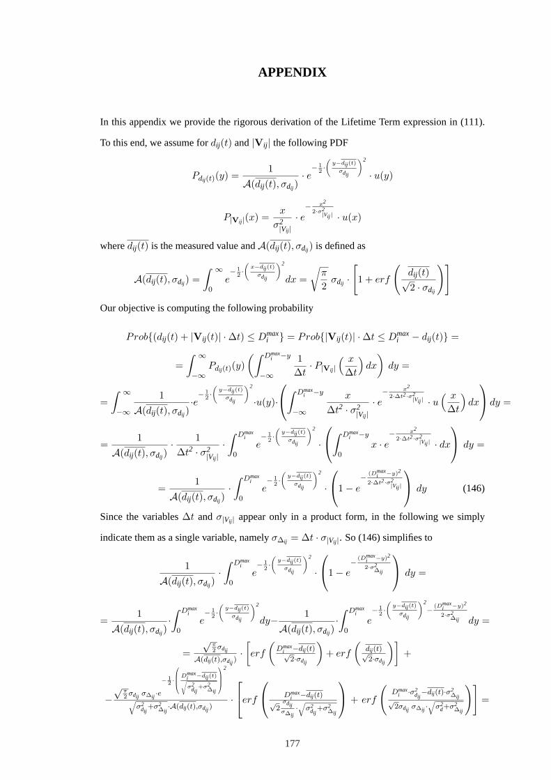
APPENDIX
In this appendix we provide the rigorous derivation of the Lifetime Term expression in (111).
To this end, we assume fordij (t) and|Vij | the following PDF
Pdij (t)(y) =1
A(dij (t), σdij )· e− 1
2·(
y−dij (t)
σdij
)2
· u(y)
P|Vij |(x) =x
σ2|Vij |
· e− x2
2·σ2|Vij | · u(x)
wheredij (t) is the measured value andA(dij (t), σdij ) is defined as
A(dij (t), σdij ) =∫ ∞
0e− 1
2·(
x−dij (t)
σdij
)2
dx =√
π
2σdij ·
[1 + erf
(dij (t)√2 · σdij
)]
Our objective is computing the following probability
Prob(dij (t) + |Vij (t)| ·∆t) ≤ Dmaxi = Prob|Vij (t)| ·∆t ≤ Dmax
i − dij (t) =
=∫ ∞
−∞Pdij (t)(y)
(∫ Dmaxi −y
−∞
1∆t
· P|Vij |( x
∆t
)dx
)dy =
=∫ ∞
−∞
1A(dij (t), σdij )
·e− 1
2·(
y−dij (t)
σdij
)2
·u(y)·
∫ Dmaxi −y
−∞
x
∆t2 · σ2|Vij |
· e− x2
2·∆t2·σ2|Vij | · u
( x
∆t
)dx
dy =
=1
A(dij (t), σdij )· 1∆t2 · σ2
|Vij |·∫ Dmax
i
0e− 1
2·(
y−dij (t)
σdij
)2
·
∫ Dmaxi −y
0x · e
− x2
2·∆t2·σ2|Vij | · dx
dy =
=1
A(dij (t), σdij )·∫ Dmax
i
0e− 1
2·(
y−dij (t)
σdij
)2
·1− e
− (Dmaxi −y)2
2·∆t2·σ2|Vij |
dy (146)
Since the variables∆t andσ|Vij | appear only in a product form, in the following we simply
indicate them as a single variable, namelyσ∆ij = ∆t · σ|Vij |. So (146) simplifies to
1A(dij (t), σdij )
·∫ Dmax
i
0e− 1
2·(
y−dij (t)
σdij
)2
·1− e
− (Dmaxi −y)2
2·σ2∆ij
dy =
=1
A(dij (t), σdij )·∫ Dmax
i
0e− 1
2·(
y−dij (t)
σdij
)2
dy− 1A(dij (t), σdij )
·∫ Dmax
i
0e− 1
2·(
y−dij (t)
σdij
)2
− (Dmaxi −y)2
2·σ2∆ij dy =
=√
π2σdij
A(dij (t),σdij )·[erf
(Dmax
i −dij (t)√2·σdij
)+ erf
(dij (t)√2·σdij
)]+
−√
π2σdij σ∆ij ·e
− 12 ·
Dmaxi −dij (t)√σ2
dij+σ2
∆ij
2
√σ2
dij+σ2
∆ij·A(dij (t),σdij )
·erf
Dmax
i −dij (t)√2
σdijσ∆ij
·√
σ2dij
+σ2∆ij
+ erf
(Dmax
i ·σ2dij−dij (t)·σ2
∆ij√2σdij σ∆ij ·
√σ2
d+σ2∆ij
)]=
177

=erf
(Dmax
i −dij (t)√2·σdij
)+erf
(dij (t)√2·σdij
)
1+erf
(dij (t)√2·σdij
) − σ∆ij ·e− 1
2 ·
Dmaxi −dij (t)√σ2
dij+σ2
∆ij
2
√σ2
dij+σ2
∆ij·[1+erf
(dij (t)√2·σdij
)] ·
·[erf
((Dmax
i −dij (t))·σ∆ij√2σdij ·
√σ2
dij+σ2
∆ij
)+ erf
(Dmax
i ·σ2dij−dij (t)·σ2
∆ij√2σdij σ∆ij ·
√σ2
dij+σ2
∆ij
)](147)
Eq. (147) is the final expression of the Lifetime Term, the same it appears in (111).
178

LIST OF ACRONYMS
4G Fourth Generation
AF Assured Forwarding
AODV Ad hoc On-demand Distance Vector
BFS Breadth First Search procedure
BS Base Station
CAC Connection Admission Control
CBT Core Based Protocol
CDF Cumulative Distribution Function
CL Controlled Load
DAMA Demand Assigned Multiple Access
DiffServ Differentiated Service
DIMRO DiffServ-Integrated Multicast algorithm for Internet Resource Optimization
DIMRO-GS DiffServ-Integrated Multicast algorithm for Internet Resource Optimization in
Group Shared applications
DREAM Distance Routing Effect Algorithm for Mobility
DSDV Destination Sequenced Distance Vector
DSR Dynamic Source Routing
DVB Digital Video Broadcast
DVB-RCS DVB Return Channel via Satellite
ECR Exponential Correlated Random
EDF Earliest Deadline First
179

EF Expedited Forwarding
E-RWM Extended-Random Walk Model
ETSI European Telecommunications Standards Institute
FIFO First Input First Output
FLC Fuzzy Logic Control
FTM Feasible solutions using adapted TM
FTP File Transfer Protocol
GEO Geostationary Earth Orbit
GPRS General Packet Radio Service
GPS Global Positioning System
GS Guaranteed Service
GSM Global System for Mobile Communications
HLR Home Location Register
HS Hub Station
ID IDentification number
IEEE Institute of Electrical and Electronics Engineers
IETF Internet Engineering Task Force
ILP Integer Linear Programming
INTMOD International Mobility Model
IP Internet Protocol
ISDN Integrated Service Digital Network
IST Information Society and Technology
ITAMAR Independent-Tree Ad hoc Multicast Routing
180

ITU International Telecommunications Union
KR Topology Knowledge Range
LAN Local Area Network
LAR Location-Aided Routing
MAC Medium Access Control
MANET Mobile Ad Hoc Network
METMOD Metropolitan Mobility Model
MMPP Markov Modulated Poisson Process
MN Mobile Node
MSC Mobile Switching Center
NATMOD National Mobility Model
NCC Network Control Center
OSTP Optimal solution of the Steiner Tree Problem
PAST-DM Progressively Adapted Sub-Tree in Dynamic Mesh
PDF Probability Density Function
PID Proportional-Integral-Derivative
PLL Phase-Locked Loop
PPMA Probabilistic Predictive Multicast Algorithm
PRADA PRobe-bAsed Distributed protocol for knowledge rAnge adjustment
PSTN Public Switched Telephone Network
PTKF Partial Topology Knowledge Forwarding
QoS Quality of Service
RDM Random Direction Model
181

RPGM Reference Point Group Mobility
RVGM Reference Velocity Group Mobility
RWP Random Waypoint Mobility Model
SATIP6 SATellite broadband multimedia system for IPv6
SPN Steiner tree Problem in Networks
ST Satellite Terminal
TCP Transmission Control Protocol
TM Takahashi-Matsuyama approximation for the Steiner problem in graphs
UDP User Datagram Protocol
UMTS Universal Mobile Telecommunication System
UT User Terminal
VCO Voltage Controlled Oscillator
VLR Visitor Location Register
WLAN Wireless Local Area Network
WRP Wireless Routing Protocol
xDSL Digital Subscriber Line
ZRP Zone Routing Protocol
182

REFERENCES
[1] OPNET, http://www.opnet.com/.
[2] CPLEX, http://www.cplex.com/.
[3] “SATIP6 project, Information Society and Technology programme, IST-2001-34344.”
[4] “Digital Video Broadcasting (DVB): interaction channel for satellite distribution sys-tems,” tech. rep., ETSI EN 301 790 v1.2.2, December 2000.
[5] “TIPHON: Definition of QoS classes,” tech. rep., ETSI TS 101 329-2, July 2000.
[6] A. BAR-NOY, I. K. and SIDI , M., “Mobile users: To update or not to update?,”ACM/Baltzer Wireless Networks, vol. 1, no. 2, pp. 175–185, 1995.
[7] ACAR, G. andROSENBERG, C., “Algorithms for bandwidth on demand,” inProc. of 5thKa band Utilization Conference, (Taormina, Italy), October 1999.
[8] ACAR, G. and ROSENBERG, C., “Weighted fair bandwidth-on-demand (WFBoD) forgeostationary satellite networks with on-board processing,”Comput. Networks, vol. 39,no. 1, pp. 5–20, 2002.
[9] AHUJA, R. K., MAGNANTI , T. L., andORLIN , J. B., Network Flows: Theory, Algo-rithms, and Applications. Prentice Hall, 1993.
[10] AKYILDIZ , I. F., HO, S. M., andL IN , Y. B., “Movement-based location update andselective paging for PCS networks,”IEEE/ACM Trans. on Networking, vol. 4, pp. 629–639, August 1996.
[11] AKYILDIZ , I. F., L IN , Y. B., LAI , W. R., andCHEN, R. J., “A new random walk modelfor PCS networks,”IEEE Journal on Selected Areas in Communications, vol. 18, no. 7,pp. 1254–1260, 2000.
[12] AKYILDIZ , I. F., SU, W., SANKARASUBRAMANIAM , Y., and CAYIRCI , E., “Wire-less Sensor Networks: A Survey,”Computer Networks (Elsevier) Journal, pp. 393–422,March 2002.
[13] ALMQUIST, P., “Type of Service in the Internet Protocol Suite,” tech. rep., IETF RFC1349, July 1992.
[14] ALPCAN, T. and BASAR, T., “A Variable Rate model with QoS Guarantees for Real-Time Internet Traffic,” inProc. SPIE Internat. Symp. on Information Technologies,vol. 2411, (Boston, MA), November 2000.
[15] ALTMAN , E.andBASAR, T., “Multi-User Rate-Based Flow Control,”IEEE/ACM Trans-actions on Communications, vol. 47, pp. 940–949, July 1998.
[16] ARON, I. D. and GUPTA, S., “Analytical Comparison of Local and End-to-End ErrorRecovery in Reactive Routing Protocols for Mobile Ad Hoc Networks,”Proc. ACMWorkshop Modeling, Analysis, and Simulation of Wireless and Mobile Systems (MSWiM),2000.
183

[17] ASTROM, K. J.andHAGGLUND, T., Automatic Tuning of PID controllers. North Caro-line: Instrument Society of America, 1988.
[18] ASTROM, K. J. and HAGGLUND, T., PID Controllers: Theory, Design and Tuning.North Caroline: Instrument Society of America, 1995.
[19] BAJI’ C, V. B., “Simple rule-based and fuzzy controllers,” tech. rep., TR95-07, ControlLaboratory, Technikon Natal, RSA, 1995.
[20] BALLARDIE , T., “Core Based Trees (CBT version 2) Multicast Routing,” tech. rep., IETFRFC 2189, September 1997.
[21] BALLARDIE , T., FRANCIS, P., andCROWCROFT, J., “Core Based Trees (CBT): An Ar-chitecture for Scalable Inter-Domain Multicast Routing,”Comp. Commun. Rev., vol. 23,pp. 85–95, October 1993.
[22] BALLARDIE , T., FRANCIS, P., and CROWCROFT, J., “Core Based Trees (CBT) andArchitecture for Scalable Inter-domain Multicast Routing,” inProceedings of ACM SIG-COMM’93, (San Francisco, USA), September 1993.
[23] BASAGNI, S., CHLAMTAC , I., SYROTIUK , V. R., andWOODWARD, B. A., “A distancerouting effect algorithm for mobility (DREAM),”In ACM/IEEE International Confer-ence on Mobile Computing and Networking (Mobicom98), pp. 76–84, 1998.
[24] BASAR, T. andSRIKANT, R., “Revenue-Maximizing Pricing and Capacity Expansion ina Many-Users Regime,” inProc. of IEEE INFOCOM’02, (New York, USA), pp. 1556–1563, June 2002.
[25] BECCHETTI, L., DELLI PRISCOLI, F., MAHONEN, P., MUNOZ, L., and INZERILLI ,T., “Enhancing IP Service Provision over Heterogeneous Wireless Networks: a Path To-wards 4G,”IEEE Communications Magazine, Special Issue on “Life after Third Gener-ation Mobile Communications”, vol. 39, pp. 74–81, August 2001.
[26] BERGAMO, M., “System design specification for mobile multimedia wireless network(MMWN),” Technical report, DARPA project DAAB07-95-C-D156, October 1996.
[27] BETTSTETTER, C., “Mobility Modeling in Wireless Networks: Categorization, SmoothMovement, and Border Effects,”ACM Mobile Comp. and Comm. Rev., vol. 2, no. 3, 2001.
[28] BETTSTETTER, C., “On the Minimum Node Degree and Connectivity of a Wireless Mul-tihop Network,”Proceedings of ACM Int. Symp. Mobile Ad Hoc Netw. and Comp. (Mo-biHoc), June 2002.
[29] BETTSTETTER, C. andKRAUSE, O., “On Border Effects in Modeling and Simulation ofWireless Ad Hoc Networks,”Proceedings of IEEE Int. Conf. Mobile and Wireless Comm.Networking (MWCN), 2001.
[30] BETTSTETTER, C., RESTA, G., andSANTI , P., “The Node Distribution of the RandomWaypoint Mobility Model for Wireless Ad Hoc Networks,”IEEE TRANSACTIONS ONMOBILE COMPUTING, vol. 2, July-September 2003.
[31] BETTSTETTER, C. and WAGNER, C., “The Spatial Node Distribution of the RandomWaypoint Model,” Proceedings of First German Workshop Mobile Ad Hoc Networks(WMAN), 2002.
[32] BHATTACHARYYA , S., KUROSE, J., andTOWSLEY, D., “Efficient Multicast Flow Con-trol using Multiple Multicast Groups,” tech. rep., CMPSCI, TR 97-15, March 1997.
184

[33] BIRK , Y. andCRUPNICOFF, D., “A Multicast Transmission Schedule for Scalable Multi-Rate Distribution of Bulk Data using Non-Scalable Erasure-correcting Codes,” inPro-ceedings of INFOCOM’03, (San Francisco, USA), July 2003.
[34] BLAKE , N. K., BAKER, S., andBLACK , D., “Definition of the Differentiated ServicesField (DS Field) in the IPv4 and IPv6 Headers,” tech. rep., IETF RFC 2474, December1998.
[35] BLAKE , N. K., BLACK , D., CARLSON, D., DAVIES, M., WANG, E., andWEISS, W.,“An Architecture for Differentiated Services,” tech. rep., IETF RFC 2475, December1998.
[36] BLOUGH, D. M., RESTA, G., andSANTI , P., “A Statistical Analysis of the Long-RunNode Spatial Distribution in Mobile Ad Hoc Networks,”Proceedings of ACM Int. Work-shop Modeling, Analysis, and Simulations of Wireless and Mobile Systems (MSWiM),2002.
[37] BOCHE, H. andJUGL, E., “Extension of ETSI’s mobility models for UMTS in order toget more realistic results,”In Proc. UMTS Workshop, Gtinzburg, Germany, November1998.
[38] BRADEN, R., CLARK , D., andSHENKER, S., “Integrated Services in the Internet Archi-tecture: An Overview,” tech. rep., IETF RFC 1633, July 1994.
[39] BROCH, J., MALTZ , D. A., JOHNSON, D. B., HU, Y. C., andJETCHEVA, J., “A perfor-mance comparison of multi-hop wireless ad hoc network routing protocols,”In Proceed-ings of ACM Intern. Conf. on Mobile Computing and Networking (MobiCom), October1998.
[40] CALVERT, K., DOAR, M., andZEGURA, E., “Modeling Internet Topology,”IEEE Com-munications Magazine, vol. 35, pp. 160–163, June 1997.
[41] CHANG, J. andTASSIULAS, L., “Energy Conserving Routing in Wireless Ad-hoc Net-works,” in Proceedings of IEEE INFOCOM’00, (Tel Aviv, Israel), pp. 22–31, 2000.
[42] CHENG, C., RILEY, R., KUMAR , S. P. R., and GARCIA-LUNA-ACEVES, J. J., “Aloop-free Bellman-Ford routing protocol without bouncing effect,” inin Proceedings ofACM SIGMETRICS’89, (Oakland, California, USA), pp. 224–237, ACM Press, Septem-ber 1989.
[43] CHIANG , C., “Wireless Network Multicasting,”Ph.D. dissertation, University of Cali-fornia, Los Angeles, Department of Computer Science, May 1998.
[44] CLAUS, A. andMACULAN , N., “Une nouvelle formulation du Probleme de Steiner surun graphe,” tech. rep., Centre de Recerche sur les Transports, Universite de Montreal,1983.
[45] COCK, K. D. andGESTEL, T. V., “Identification of the Circulant Modulated Poisson,”in Proceedings of the Mathematics Theory of Networks and Systems, Symposium NTNS,pp. 742–779, December 1998.
[46] COCK, K. D., GESTEL, T. V., andMOOR, B. D., “Stochastic System Identification forATM Network Traffic Models: a Time Domain Approach,” tech. rep., Internal Report K.U., (Leven-Belgium), July 1997.
185
[47] COLOMBO, G., “Mobility models for mobile system design and dimensioning,”In Proc.ITC Specialists Seminar: Teletraffic Modelling and Measurement in Broadband and Mo-bile Communications, Leidschendam, Netherlands, November 1995.
[48] DAS, S., CASTANEDA, R., YAN , J., andSENGUPTA, R., “Comparative performanceevaluation of routing protocols for mobile, ad hoc networks,”In 7th Int. Conf. on Com-puter Communications and Networks (IC3N), p. 153161, October 1998.
[49] DAS, S. R., PERKINS, C. E., and ROYER, E. M., “Performance comparison of twoon-demand routing protocols for ad hoc networks,”Proceedings of IEEE INFOCOM, TelAviv, Israel, 2000.
[50] DAS, S. R., PERKINS, C. E., ROYER, E. M., and MARINA , M. K., “Performancecomparison of two on-demand routing protocols for ad hoc networks,”IEEE PersonalCommunications, February 2001.
[51] DEBRAY, A., “SATIP6 project Scenarios,” inProceedings of IST 2003, (Aveiro, Portu-gal), June 2003.
[52] DELLI PRISCOLI, F., “Design and Implementation of a Simple and Efficient MediumAccess Control for High Speed Wireless Local Area Networks,”IEEE Journal on Se-lected Areas in Communications (JSAC), vol. 17, pp. 2052–2064, November 1999.
[53] DELLI PRISCOLI, F.andISIDORI, A., “A Control-Engineering Approach to Traffic Con-trol in Wireless Networks,” inProc. of the Conference on Decision and Control (DCD),(Las Vegas, USA), December 2002.
[54] DELLI PRISCOLI, F. andPIETRABISSA, A., “Control-theoretic Band-on-Demand Pro-tocol for Satellite Networks,” inProc. of Conference on Control Applications (CCA),(Glasgow (UK)), September 2002.
[55] DELLI PRISCOLI, F. and PIETRABISSA, A., “Resource Management for ATM BasedGeostationary Satellite Networks with On-Board Processing,”Computer Networks, Else-vier Science Pub., vol. 39, no. 1, pp. 43–60, 2002.
[56] DELLI PRISCOLI, F., POMPILI , D., andSETTE, G., “A Control Theory based MediumAccess Control for the downstream satellite uplink of SATIP6 project,” inProceedingsof ECC 2003, (Cambridge, United Kindom), September 2003.
[57] DELLI PRISCOLI, F., POMPILI , D., andSANTORO, G., “A QoS-aware Bandwidth onDemand Assignment Mechanism in a GEO Satellite System,” inProceedings of IST 2004,(Lyon, France), June 2004.
[58] EBERSPACHER, J., VOGEL, H. J., andBETTSTETTER, C., GSM - Switching, Servicesand Protocols. John Wiley&Sons, 2nd edition, March 2001.
[59] ESTRIN, D., GOVINDAN , R., HEIDEMANN , J., andKUMAR , S., “Next Century Chal-lenges: Scalable Coordination in Sensor Networks,” inProceedings of IEEE/ACM Mobi-com, (Seattle, USA), pp. 263–270, 1999.
[60] ETSI, “Selection procedures for the choice of radio transmission technologies of theUMTS (UMTS 30.03, version 3.2.0),”Technical report, European TelecommunicationStandards Institute, April 1998.
[61] FANG, Y., CHLAMTAC , I., andL IN , Y. B., “Portable movement modeling for PCS net-works,” IEEE Trans. on Vehicular Technology, vol. 49, July 2000.
186

[62] FANG, Y., CHLAMTAC , I., andL IN , Y., “Channel occupancy times and handoff rate formobile computing and PCS networks,”IEEE Trans. on Computers, vol. 47, June 1998.
[63] FINN , G. G., “Routing and Addressing Problems in Large Metropolitan-Scale Internet-works,” tech. rep., ISI res. rep ISU/RR- 87-180, March 1987.
[64] FOURER, R., GAY, D. M., andKERNIGHAN, B. W., AMPL: A Modeling Language forMathematical Programming. Duxbury Press, Cole Publishing Co., 2002.
[65] FRANCIOSA, P. G., FRIGIONI, D., and GIACCIO, R., “Semi-dynamic shortest pathsand breadth-first search on digraphs,” inin Symp. on Theoretical Aspects of ComputerScience, Comp. Sc. 1200, pp. 33–46, 1997.
[66] GAREY, M. R. andJOHNSON, D. S., Computer and Intractability. W. H. Freeman andCo., 1979.
[67] GERAKOULIS, D., “Demand assignment control in a satellite switched CDMA network,”Int. J. Netw. Manag., vol. 10, no. 4, pp. 175–189, 2000.
[68] GOLDSMITH, A. J., “Variable-Rate Variable-Power MQAM for Fading Channels,” inProceedings of IEEE Vehicular Technology Conference, (Atlanta, GA, USA), pp. 815–819, April 1996.
[69] GOLDSMITH, A. J. andCHUA , S.-G., “Variable-Rate Variable-Power MQAM for Fad-ing Channels,”IEEE Transactions on Communications, vol. 45, pp. 1218–1230, October1997.
[70] GROSS, J. L.andYELLEN, J., “Handbook of Graph Theory,”Discrete Mathematics andIts Applications, CRC Press, vol. 25, 2003.
[71] GROSSGLAUSER, M. andTSE, D., “Mobility Increases the Capacity of Ad Hoc WirelessNetworks,”Proc. IEEE INFOCOM’01, April 2001.
[72] GUI , C. and MOHAPATRA, P., “Efficient Overlay Multicast for Mobile Ad Hoc Net-works,” in Proceedings of IEEE WCNC’03, (New Orleans, Luoisiana, USA), March2003.
[73] GUI , C. andMOHAPATRA, P., “Scalable Multicasting in Mobile Ad Hoc Networks,” inProceedings of IEEE INFOCOM’04, (Hong Kong S.A.R., PRC), March 2004.
[74] GUPTA, P. andKUMAR , P. R., “The Capacity of Wireless Networks,”IEEE Trans. In-formation Theory, vol. 46, March 2000.
[75] GUPTA, P.andKUMAR , P., “Critical power for asymptotic connectivity in wireless net-works,” Stochastic Analysis, Control, Optimization, and Applications, 1998.
[76] GUTRIN, R. A., “Channel occupancy time distribution in a cellular radio system,”IEEETrans. on Vehicular Technology, vol. 36, pp. 89–99, August 1987.
[77] HAAS, Z. J., “A new routing protocol for the reconfigurable wireless networks,”InProc. of IEEE 6th International Conference on Universal Personal Communications(ICUPC97), p. 562566, 1997.
[78] HAAS, Z. J., “Design Methodologies for Adaptive and Multimedia Networks,”IEEECommunications Magazine, vol. 39, pp. 106–107, November 2001.
187

[79] HAAS, Z. J.andL IANG , B., “Predictive Distance-Based Mobility Management for PCSNetworks,” IEEE Conference on Computer Communications (INFOCOM99), March1999.
[80] HAAS, Z. J. andPEARLMAN , M. R., “The performance of query control schemes forthe Zone Routing Protocol,”In Proceedings of ACM SIGCOMM, Vancouver, Canada,September 1998.
[81] HEINANEN, J., BAKER, F., WEISS, W., andWROCLAWSKI, J., “Assured ForwardingPHB Group,” tech. rep., IETF RFC 2597, June 1999.
[82] HEINZELMAN , W., Application-Specific Protocol Architectures for Wireless Networks.Ph.d. thesis, Massachusetts Institute of Technology, 2000.
[83] HEINZELMAN , W. B., CHANDRAKASAN , A., and BALAKRISHNAN , H., “AnApplication-Specific Protocol Architecture for Wireless Microsensor Networks,”IEEETransactions on Wireless Communications, vol. 1, pp. 660–670, October 2002.
[84] HIGHTOWER, J. andBORRIELLO, G., “Location Systems for Ubiquitous Computing,”IEEE Computers, pp. 14–25, August 2001.
[85] HONG, D. andRAPPAPORT, S. S., “Traffic model and performance analysis for cellularmobile radio telephone systems with prioritized and nonprioritized handoff procedures,”IEEE Trans. on Vehicular Technology, vol. 35, pp. 77–92, August 1986.
[86] HONG, X., GERLA, M., PEI, G., andCHIANG , C., “A Group Mobility Model for AdHoc Wireless Networks,”ACM International Workshop on Modeling and Simulation ofWireless and Mobile Systems (MSWiM99), August 1999.
[87] HOU, T. C. andL I , V. O. K., “Transmission Range Control in multihop packet radionetworks,”IEEE Transactions on Communications, vol. 34, pp. 38–44, January 1986.
[88] HU, R. Q. andPETR, D. W., “A predictive self-tuning fuzzy-logic feedback rate con-troller,” IEEE/ACM Trans. Netw., vol. 8, no. 6, pp. 697–709, 2000.
[89] INZERILLI , T. andPOMPILI , D., “Towards a new generation of IP-based satellites,” inProceedings of IST 2002, (Copenhagen, Denmark), November 2002.
[90] JACOBSON, V., NICHOLS, K., andPODURI, K., “An Expedited Forwarding PHB,” tech.rep., IETF RFC 2598, June 1998.
[91] JAIN , R., PURI, A., andSENGUPTA, R., “Geographical Routing Using Partial Infor-mation for Wireless Ad Hoc Networks,”IEEE Personal Communications, pp. 48–57,February 2001.
[92] JIANG , T., AMMAR , M. H., and ZEGURA, E. W., “Inter-receiver fairness: A novelperformance measure for multicast ABR sessions,” inin Proceedings of ACM SIGMET-RICS’98, (Madison, Wisconsin, USA), June 1998.
[93] JIANG , Z., L I , Y., and LEUNG, V. C. M., “A predictive demand assignment multi-ple access protocol for broadband satellite networks supporting Internet applications,” inProceedings of IEEE ICC, vol. 5, (New York, USA), pp. 2973–2977, May 2002.
[94] JOHANSSON, R., LARSSON, T., HEDMAN , N., M IELCZAREK, B., andDEGERMARK,M., “Scenario-based performance analysis of routing protocols for mobile ad-hoc net-works,” In Proceedings of ACM Intern. Conf on Mobile Computing and Networking (Mo-biCom), Seattle, USA, August 1999.
188

[95] JOHNSON, D. B. and MALTZ , D. A., “Dynamic Source Routing in ad hoc wirelessnetworks,”Kluwer Academic Publishers, 1996.
[96] K IM , T. S., KWON, J. K., andSUNG, D. K., “Mobility and traffic analysis in three-dimensional high rise building environments,”IEEE Trans. on Vehicular Technology,vol. 49, pp. 1633–1640, May 2000.
[97] KO, Y. B. and VAIDYA , N. H., “Location-aided routing(LAR) in mobile ad hoc net-works,” In ACM/IEEE International Conference on Mobile Computing and Networking(Mobicom98), 1998.
[98] KRANAKIS , E., SINGH, H., and URRUTIA, J., “Compass routing on geometric net-works,” in Proceedings of the 11-th Canadian Conference on Computational Geometry,(Vancouver, Canada), August 1999.
[99] LAM , D., COX, D. C., andWIDOM , J., “Teletraffic modeling for personal communica-tion services,”IEEE Communications Magazine, vol. 35, pp. 79–87, October 1997.
[100] LAWSON, C. andHANSON, R., “Solving least square problem,”Classic Applied Mathe-matics Series, vol. 15, 1995.
[101] LEUNG, K., MASSEY, W., andWHITT, W., “Traffic Models for Wireless Communica-tion Networks,”Journal on Selected Areas in Communications, pp. 1353–1364, October1994.
[102] L I , J., JANNOTTI , J., COUTO, D. D., KARGER, D., andMORRIS, R., “A Scalable Lo-cation Service for Geographic Ad Hoc Routing,” inProceedings of IEEE/ACM Mobicom,pp. 120–130, 2000.
[103] L ICHTENSTEIN, D., “Planar Formuale and their use,”SIAM Journal on Computing,vol. 11, pp. 329–343, May 1982.
[104] L IN , D. and AKUJOBI, F., “Differentiated Service Router Architecture-Classification,Metering and Policing,” tech. rep., WFQ, July 2000.
[105] L IN , Y. B., “Performance modeling for mobile telephone networks,”IEEE Network,pp. 63–67, November 1997.
[106] L IN , Y. B., “Reducing location update cost in PCS network,”IEEE/ACM Trans. on Net-working, vol. 5, pp. 25–33, February 1997.
[107] LOW, C. P.andWANG, N., “On Finding Feasible solutions to Group Multicast RoutingProblem,” IEICE Transactions on Communications, vol. E85-B, pp. 268–277, January2002.
[108] LU, C., STANKOVIC , J. A., TAO, G., andSON, S. H., “Design and Evaluation of aFeedback Control EDF Scheduling Algorithm,” inProceedings of the 20th IEEE Real-Time Systems Symposium, p. 56, IEEE Computer Society, 1999.
[109] MARKOULIDAKIS , J. G., LYBEROPOULOS, G. L., TSIRKAS, D. E., andSYKAS , E. D.,“Mobility modeling in third-generation mobile telecommunication systems,”IEEE Per-sonal Communications, pp. 41–56, August 1997.
[110] MCDONALD , A. B. andZNATI , T. F., “A Path Availability Model for Wireless Ad-HocNetworks,” inProceedings of IEEE Wireless Communications and Networking Confer-ence (WCNC), (New Orleans, Luoisiana, USA), September 1999.
189

[111] MCDONALD , A. B. andZNATI , T. F., “Predicting node proximity in ad-hoc networks:a least overhead adaptive model for selecting stable routes,” inProceedings of the 1stACM international symposium on Mobile ad hoc networking & computing, (Boston, Mas-sachusetts, USA), pp. 29–33, IEEE Press, 2000.
[112] MELODIA , T., POMPILI , D., andAKYILDIZ , I. F., “Optimal Local Topology Knowledgefor Energy Efficient Geographical Routing in Sensor Networks,” inProceedings of IEEEINFOCOM 2004, (Hong Kong S.A.R., PRC), March 2004.
[113] M ITCHELL , P. D., Effective Medium Access Control for Geostationary Satellite Systems.Phd thesis, University of York, UK, 2003.
[114] MO, J. and WALRAND , J., “Fair End-to-End Window-Based Congestion Control,”IEEE/ACM Transactions on Networking, vol. 8, pp. 556–567, October 2000.
[115] MORALES-ANDREAS, G. andV ILLEN -ALTAMIRANO , M., “An approach to modelingsubscriber mobility in cellular networks,” inProceedings of 5th Worm Telecommunica-tion Forum, November 1987.
[116] NASIPURI, A., CASTANEDA, R., andDAS, S., “Performance of Multipath Routing forOn-Demand Protocols in Mobile Ad Hoc Networks,”ACM/Kluwer Mobile Networks andApplications, vol. 6, pp. 339–349, 2001.
[117] NELSON, R. andKLEINROCK, L., “The spatial capacity of a slotted ALOHA multihoppacket radio network with capture,”IEEE Transactions on Communications, vol. 32,no. 6, pp. 684–694, 1984.
[118] NICHOLS, K., JACOBSON, V., and ZHANG, L., “A Two Bit Differentiated ServicesArchitecture for the Internet,” tech. rep., IETF RFC 2638, November 1997.
[119] OFLIK , P.andRAPPAPORT, S., “A model for teletraffic performance and channel hold-ing time characterization in wireless cellular communication,” inProceedings of IEEEInternational Conference Universal Personal Communications (ICUPC), 1997.
[120] PAUL , P.andRAGHAVAN , S., “Survey of multicast routing algorithms and protocols,” inProceedings of the 15th International Conference on Computer Communication (ICCC2002), 2002.
[121] PEARLMAN , M. R., SHOLANDER, Z. J. H. E., andTABRIZI , S. S., “On the impactof alternate path routing for load balancing in mobile ad hoc networks,”In Proc. Intern.Workshop on Mobile Ad Hoc Networking and Computing (MobiHOC), August 2000.
[122] PERKINS, C. andROYER, E., “Ad hoc on-demand distance vector routing,”In Proceed-ings of the 2nd IEEE Workshop on Mobile Computing Systems and Applications, 1999.
[123] POMPILI , D., DELLI PRISCOLI, F., andSANTORO, G., “Enhanced IP-based satellitearchitecture compatible with many satellite platforms,” inProc. of the Conference ofInformation Society Technologies (IST), (The Hague), November 2004.
[124] POMPILI , D., LOPEZ, L., andSCOGLIO, C., “DIMRO, a DiffServ-Integrated Multicastalgorithm for Internet Resource Optimization in source specific multicast applications,”in Proceedings of ICC 2004, (Paris, France), June 2004.
[125] POSTEL, J., “Internet Control Message Protocol (ICMP),” tech. rep., IETF RFC 792,September 1981.
190

[126] QI , H. D., QI , L., andSUN, D., “Solving Karush-Kuhn-Tucker Systems via the TrustRegion and the Conjugate Gradient Methods,”SIAM Journal on Optimization, vol. 14,no. 2, pp. 439–463, 2003.
[127] RAMANATHAN , R. andROSALES-HAIN , R., “Topology Control of Multihop WirelessNetworks using Transmit Power Adjustement,” inProceedings of IEEE INFOCOM’00,(Tel Aviv, Israel), 2000.
[128] REXFORD, J., BONOMI, F., GREENBERG, A. G., and WONG, A., “A Scalable Ar-chitecture for Fair Leaky-Bucket Shaping,” inProc. of INFOCOM’97, pp. 1054–1062,1997.
[129] RODOPLU, V. and MENG, T., “Minimum Energy Mobile Wireless Networks,”IEEEJournal of Selected Aresas In Communications, vol. 17, pp. 1333–1344, August 1999.
[130] ROSENBERG, C., “Broadband satellite systems: a network perspective,” inProc. of IEEEGLOBECOM’00, (San Francisco, USA), November 2000.
[131] ROYER, E., MELLIAR -SMITH , P., andMOSER, L., “An Analysis of the Optimum NodeDensity for Ad hoc Mobile Networks,”In Proc. IEEE Infocom, Tel Aviv, Israel, 2000.
[132] ROYER, E. M. andPERKINS, C. E., “Multicast Operation of the Ad-Hoc On-DemandDistance Vector Routing Protocol,” inMobile Computing and Networking (MOBICOM),pp. 207–218, August 1999.
[133] RUBIN , I. andCHOI, C., “Impact of the Location Area Structure on the Performance ofSignaling Channels in Wireless Cellular Networks,”IEEE Communications Magazine,pp. 108–115, 1997.
[134] RYD , T., “An EM algorithm for estimation in Markov-Modulated Poisson Processes,”Comput. Stat. Data Anal., Elsevier Science Pub., vol. 21, no. 4, pp. 431–447, 1996.
[135] SAHASRABUDDHE, L. H. and MUKHERJEE, B., “Multicast Routing Algorithms andProtocols: A Tutorial,”IEEE Network, vol. 14, pp. 90–102, January/February 2000.
[136] SAJAMA andHAAS, Z. J., “Independent-tree ad hoc multicast routing (ITAMAR),”Mob.Netw. Appl., vol. 8, no. 5, pp. 551–566, 2003.
[137] SAKAMOTO , T., KAMAGATA , E., andSERIZAWA , M., “Location registration and pagingfor in-building personal multi-media communication systems,” inProceedings of IEEEVehicular Technology Conf., 1996.
[138] SANCHEZ, M., “Mobility Models,” http://www.disca.upv.es/misan/mobmodel.htm,November 2000.
[139] SANCHEZ, M. and MANZONI , P., “A Java-Based Ad Hoc Networks Simulator,”SCSWestern Multiconference Web-based Simulation Track, San Francisco, January 1999.
[140] SANTI , P. andBLOUGH, D. M., “The Critical Transmitting Range for Connectivity inSparse Wireless Ad Hoc Networks,”IEEE Trans. Mobile Computing, vol. 2, pp. 25 – 39,Jan.-Mar. 2003.
[141] SCHOPP, M., “User modeling and performance evaluation of distributed location man-agement for personal communications services,”In Proc. Intern. Teletraffic Congress,Washington, USA, June 1997.
191

[142] SCOURIAS, J. andKUNZ, T., “An activity-based mobility model and location manage-ment simulation framework,”In Proc. ACM Intern. Workshop on Modeling, Analysis, andSimulation of Wireless and Mobile Systems (MSWiM), Seattle, August 1999.
[143] SHAKHASHIRI , B., “Random Walk,”http://scifun.chem.wisc.edu/WOP/RandomWalk.html,November 2000.
[144] STOJMENOVIC, I., “Position-Based Routing in Ad Hoc Networks,”IEEE Communica-tions Magazine, vol. 40, pp. 128–134, July 2002.
[145] SUGENO, M., An Introductory Survey of Fuzzy Control. Information Science, 1985.
[146] TAKAGI , H. and KLEINROCK, L., “Optimal Transmission Ranges for Randomly Dis-tributed Packet Radio Terminals,”IEEE Transactions on Communications, vol. 32, no. 3,pp. 246–57, 1984.
[147] TAKAHASHI , H. andMATSUYAMA , A., “An approximate solution for the Steiner prob-lem in graphs,”Math. Japonica, vol. 6, pp. 573–577, 1980.
[148] THOMAS, R., GILBERT, H., andMAZZIOTTO, G., “Influence of the moving of the mo-bile stations on the performance of a radio mobile cellular network,”In Proc. Nordic Sem-inar on Digital Land Mobile Radio Communications, Copenhagen, Denmark, September1988.
[149] TOBAGI, F. A. andKLEINROCK, L., “Packet switching in radio channels: part II - Thehidden terminal problem in carrier multiple-access and the busy-tone solution,”IEEETransactions on Communications, vol. COM-23, pp. 1417–1433, December 1975.
[150] WANG, K. H. andL I , B., “Group Mobility and Partition Prediction in Wireless Ad-HocNetworks,”IEEE, 2002.
[151] WANG, N. andLOW, C. P., “On Finding Feasible solutions to Group Multicast RoutingProblem,” inProceedings of IFIP International Conference of NETWORKING’00, (Paris,France), May 2000.
[152] WAXMAN , B. M., “Routing of multipoint connections,”IEEE Journal on Selected Areasin Communications, vol. 6, pp. 1617–1622, December 1988.
[153] WEISSTEIN, E., “Polya’s Random Walk Constants,” Wolfram Research,http://mathworld.wolfram.com/PolyasRandomWalkConstants.html, May 2000.
[154] WONG, R. T., “A dual ascent approach for Steiner tree problems on a directed graph,”Mathematical Programming, vol. 28, pp. 271–287, 1984.
[155] WOO, S. M., SINGH, S., andRAGHAVENDRA , C. S., “Power-Aware Routing in MobileAd Hoc Networks,” inProceedings of IEEE/ACM Mobicom, pp. 513–529, 1998.
[156] YAICHE, H., MAZUMDAR , R. R., andROSENBERG, C., “A Game Theoretic Frameworkfor Bandwidth Allocation and Pricing in Broadband Networks,”IEEE/ACM Transactionson Networking, vol. 8, pp. 667–678, October 2000.
[157] ZADEH, L. A., “A rationale for fuzzy control,”J. Dynamic Syst. Meas. Control, vol. 94,pp. 3–4, 1972.
[158] ZADEH, L. A., “Outline of a new approach to the analysis of complex systems anddecision processes,”IEEE Trans. Syst., Man., Cyber., vol. SMC-3, no. 1, pp. 28–44,1973.
192

[159] ZADEH, L. A., “Fuzzy logic,” IEEE Computer Mag., vol. SMC-3, pp. 83–93, April 1988.
[160] ZONOZZI, M. M. andDASSANAYAKE , P., “Mobility modeling and channel holding timedistribution in cellular mobile communication systems,” inProceedings of IEEE Globe-com, 1995.
[161] ZONOZZI, M. M. andDASSANAYAKE , P., “User mobility modeling and characterizationof mobility patterns,”IEEE Journal on Sel. Areas in Communications, vol. 15, pp. 1239–1252, September 1997.
193

VITA
Dario Pompili was born in Rome, Italy, in 1977. He received the “Laurea” degree in Telecom-
munications Engineering in 2001, magna cum laude, from the University of Rome “La Sapienza”,
Italy, with a thesis titled “Quality of Service in a broad band satellite network for Internet ac-
cess”. The thesis, developed within the BRAHMS (BRoadband Access for High speed Multime-
dia via Satellite) Project, promoted by IST (Information Society of Technologies) and financed
by EU, focused on the study and development of an IP Traffic Control to integrate IntServ
(Inegrated Service) and DiffServ (Differentiated Service) Quality of Service (QoS) different
approaches, introduction of hard states in RSVP (ReSerVation Protocol) to limit the amount
of RSVP protocol signaling packets in transit along the satellite path and TCP (Transmission
Control Protocol) enhancements for the satellite path.
From June 2001 he has been working at the same university on the European Union IST
BRAHMS and SATIP6 (SATellite broadband multimedia system for IPv6) projects aiming at
identifying, designing and demonstrating a new set of services and functionalities upon an inte-
grated Terrestrial and Satellite broadband network.
In 2003 he worked on Sensor Networks at the Broadband and Wireless Networking Labo-
ratory (BWN-Lab), Georgia Institute of Technology, Atlanta, as a visiting researcher. His main
research interests are in Wireless Sensor Networks, Underwater Acoustic Sensor Networks and
Quality of Service in Broadband Satellite Networks.
He attended several technical stages: i) One month at the Advanced School in Mobile Com-
puting at “Scuola Normale Superiore”, Pisa, September 2003; ii) A week in July 2002 at the
“VI National School CIRA - Centro Interuniversitario per le Ricerche in Automatica”, Bertinoro
(Italy), attending lectures on Linear Systems and Mobile Robotics; iii) Two weeks in September
2000 at “G. Reiss Romoli High School”, L’Aquila (Italy), for a technical stage organized by
Telecom Italia S.p.A., dealing with a development of a Business Plan of a tlc operator who has
to decide whether is worth entering in a new foreign market.
The following is a list of his publications, as of this writing:
• D. Pompili and M. Vittucci, “PPMA, a Probabilistic Predictive Multicast Algorithm in Ad
194

Hoc Networks”, submitted for publication, December 2004
• T. Melodia, D. Pompili, and I. F. Akyildiz, “On the Interdependence of Distributed Topol-
ogy Control and Geographical Routing in Ad Hoc and Sensor Networks”, accepted for
publication on JSAC Special Issue on Wireless Ad Hoc Networks, 2005
• I. F. Akyildiz, D. Pompili, and T. Melodia, “Challenges for Efficient Communication in
Underwater Acoustic Sensor Networks”, ACM Sigbed Review, July 2004
• D. Pompili, L. Lopez, C. Scoglio, and F. Delli Priscoli, “DiffServ-Integrated Algorithms
for Resource Optimization in Source Specific and Group Shared Multicast Applications
in Internet”, submitted for publication, May 2004
• F. Delli Priscoli and D. Pompili, “A Control-Predictive Approach to Demand-Assignment
Mechanism with QoS Guarantees in a GEO Satellite System”, submitted for publication,
November 2003
• F. Delli Priscoli, D. Pompili, and G. Sette, “A Control based Traffic Controller providing
QoS guarantees”, submitted for publication, November 2003
• D. Pompili and M. Vittucci, “A Probabilistic Predictive Multicast Algorithm in Ad Hoc
Networks (PPMA)”, proceedings of Med-Hoc-Net 2004
• D. Pompili and T. Melodia, “An architecture for ocean bottom UnderWater Acoustic Sen-
sor Networks”, proceedings of Med-Hoc-Net 2004
• D. Pompili, F. Delli Priscoli, and G. Santoro, “Enhanced IP-based satellite architecture
compatible with many satellite platforms”, proceedings of IST 2004
• F. Delli Priscoli, D. Pompili, and G. Santoro, “A QoS-aware Bandwidth on Demand As-
signment Mechanism in a GEO Satellite System”, proceedings of IST 2004
• D. Pompili, L. Lopez, and C. Scoglio, “DIMRO, a DiffServ-Integrated Multicast algo-
rithm for Internet Resource Optimization in source specific multicast applications”, pro-
ceedings of ICC 2004
• T. Melodia, D. Pompili, and I. F. Akyildiz, “Optimal Local Topology Knowledge for
Energy Efficient Geographical Routing in Sensor Networks”, proceedings of INFOCOM
2004
195

• P. Dini, G. Fraietta, and D. Pompili, “Fair per-flow multi-step scheduler in a new Internet
DiffServ node architecture”, proceedings of SoftCom 2003
• F. Delli Priscoli, D. Pompili, and G. Sette, “A control based Traffic Controller in wireless
and satellite downlink channels”, proceedings of ECC 2003
• F. Delli Priscoli, D. Pompili, and G. Sette, “A Control Theory based Medium Access
Control for the downstream satellite uplink of SATIP6 project”, proceedings of IST 2003
• T. Inzerilli and D. Pompili, “Towards a New Generation of IP-based Satellites”, proceed-
ings of IST 2002
• F. Del Sorbo, G. Lombardi, and D. Pompili, “SIP based services and Virtual Home UMTS
environment in the IST research project FUTURE”, proceedings of GLOBECOM 2002
• F. Del Sorbo, G. Lombardi, and D. Pompili, “UMTS access network architecture for
multimedia services”, proceedings of IWDC 2002
• G. Fraietta, T. Inzerilli, V. Morsella, and D. Pompili, “A DiffServIntServ Integrated QoS
Provision Approach in BRAHMS Satellite System”, proceedings of IST 2001
• Dario Pompili, “Quality of Service in a broad band satellite network for Internet access”,
Laurea Thesis (MS Thesis), University of Rome, “La Sapienza”, May 2001, (in English
with an introduction in Italian)
196
Top Related