


Languages
Pages
Legal

Dominant Retailers’ Incentives for Product Quality
Feb 18, 2010
Anthony Dukes
Marshall School of Business University of Southern California
Los Angeles CA [email protected]
Tansev Geylani Katz Graduate School of Business
University of Pittsburgh Pittsburgh PA
Yunchuan Liu College of Business
University of Illinois at Urbana-Champaign Champaign IL
Dominant Retailers’ Incentives for Product Quality
ABSTRACT
This paper investigates the diverging incentives for product quality in a channel with two asymmetric retailers and a common supplier. When retailers differ in terms of service provision and channel power, changes in manufactured quality cause channel conflicts. In particular, our results show that if the low service retailer becomes dominant in the channel, it may induce a low level of quality that is detrimental for the other members of the channel. The low service retailer benefits from quality reduction first by improving its competitive standing against its rival retailer by lessening the importance of quality for consumer choice and second by strengthening its relative bargaining position vis-à-vis its supplier. Our results also show that consumer surplus may increase as a result of quality reduction. Keywords: Product Quality; Channels of Distribution; Retailing; Dominant Retailer

1
1. Introduction
One of the controversial issues surrounding large-scale discount retailers is a concern over
product quality.1 Critics of Wal-Mart, in particular, complain not only that it sells low quality
products but, perhaps more importantly, that its size and influence may actually have detrimental
effects on quality, which go beyond the products sold within its stores.2 This paper examines the
connection between the influence on quality by certain retailers and the quality of products sold
elsewhere.
Traditionally, quality was determined exclusively by consumer product manufacturers.
Such a determination was based on market needs and manufacturer profitability. Now, however,
as has been well-documented, several large-scale retailers have acquired significant influence
over their suppliers. This influence may even extend to product specifications (Dobson and
Waterson 1999, Luo et al. 2007).3 For example, Wal-Mart is known for its influence with
manufacturers to lower product quality.4 A fundamental question this paper addresses is: why
and under what conditions does a powerful retailer try to reduce manufactured quality?
An important aspect of our research is the fact that manufacturers sell their products
through multiple retailers. Lower quality, as induced by a single powerful retailer, may therefore
1 A Consumer Reports (2002) survey of shoppers found that Wal-Mart was among the lowest in perceived quality among major retailers in the US. See also The Mirror (October 15, 2005) for criticisms of Tesco’s quality standards. 2 See anecdotal discussions of Wal-Mart’s influence on manufactured quality and the impact of this influence on its suppliers and rival retailers in Charles Fishman’s (2006) book: “The Wal-Mart Effect”. See also The Scotsman (August 26, 2005) for concerns that Tesco’s use of foreign sourced, low quality beef, which is labeled to appear locally sourced, adversely affects consumer’s general perceptions of British produced beef. 3 Fishman (2006) reports the CEO of an instantly recognizable consumer products company in an interview saying, “You know they (Wal-Mart) have a tremendous impact on innovation, on the development of new products. You know they are enormously damaging in that arena.” For instance, according his interviews with an ex-design engineer electronics manufacturer, Philips, faced with pressure from Wal-Mart, made its TV cabinets thinner and took away extra features Wal-Mart did not want (Fishman 2006). 4 According to Business Week, Wal-Mart heavily influences product specifications and is criticized by suppliers that it forces down quality standards (Bianco 2003). For example, Snapper Lawn Mowers were sold in both Wal-Mart and in specialty lawn care retailers. According to an interview with its CEO, continuing to supply Wal-Mart meant gradual but irresistible corrosion of the very qualities for which Snapper was known (Fishman 2006).

2
have an impact at other retailers supplied by the same manufacturer. If reduced quality benefits
the powerful retailer then how does it affect the other members of the channel, the manufacturer
and competing retailers? This is a second question we ask in this paper. A third and final
question asked in this research is: What are the implications for consumers when a powerful
retailer exerts its influence on quality? This question is particularly important since large
discounters are often criticized on reducing manufacturers’ quality which may become
detrimental to consumers (Fishman 2006).
The motivating premise behind our inquiry is the fact that manufacturers of nationally
branded goods typically distribute their products through competing retailers which may differ
in, among other things, the level of their service or their ability to accentuate quality features of
products. For instance, the department store chain, Sears, sells many of the same products as
Wal-Mart, yet has emphasized better product quality and better customer service than Wal-Mart
(Journal Record 1991). Similarly, retailers in the grocery industry, such as H-E-B and Wegmans,
are acclaimed for introducing lavish displays in order to highlight quality attributes of many
national brands, which are also sold at large discounters.5 Furthermore, while discounters are
subject to complaints about customer service,6 these smaller, regional retailers emphasize their
commitment to customer service.7
It is perhaps not surprising that smaller retailers are differentiated from their larger rivals.
What is not so obvious is the implication of these differences for the channel relationships vis-à-
vis their common suppliers. The examples above illustrate the asymmetric nature of retail
competition, which is crucial for understanding the diverging incentives for product quality.
5 See, for example HBS Case, H-E-B Own Brands and Fortune article “The Wegmans Way” (Boyle et al. 2005). 6 See, for example, consumeraffairs.com (http://www.consumeraffairs.com/retail/walmart.htm). 7 See, again, HBS Case, H-E-B Own Brands and Fortune article “The Wegmans Way (Boyle et al. 2005).
3
And, depending on the power structure of the channel, these differences have implications for the
level of quality produced, prices paid, and the corresponding welfare of consumers.
Our analysis is based on a game-theoretical model in which two asymmetric retailers
compete for the sale of a single product supplied by a common manufacturer. Under the premise
that the retailers differ with respect to their channel power and level of service, we first show that
if the low service retailer (e.g. a discounter) has more channel power over the manufacturer
(dominant) than the high service retailer (weak), then the dominant retailer benefits from a
reduction in manufactured quality.
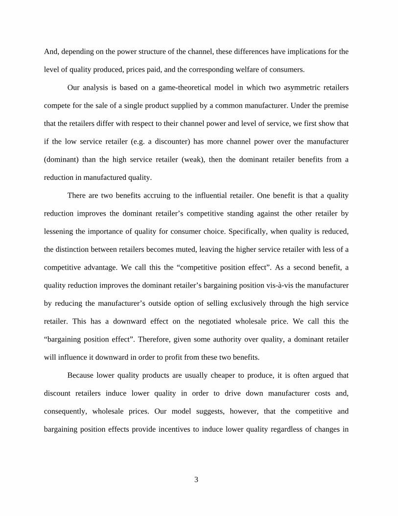
There are two benefits accruing to the influential retailer. One benefit is that a quality
reduction improves the dominant retailer’s competitive standing against the other retailer by
lessening the importance of quality for consumer choice. Specifically, when quality is reduced,
the distinction between retailers becomes muted, leaving the higher service retailer with less of a
competitive advantage. We call this the “competitive position effect”. As a second benefit, a
quality reduction improves the dominant retailer’s bargaining position vis-à-vis the manufacturer
by reducing the manufacturer’s outside option of selling exclusively through the high service
retailer. This has a downward effect on the negotiated wholesale price. We call this the
“bargaining position effect”. Therefore, given some authority over quality, a dominant retailer
will influence it downward in order to profit from these two benefits.
Because lower quality products are usually cheaper to produce, it is often argued that
discount retailers induce lower quality in order to drive down manufacturer costs and,
consequently, wholesale prices. Our model suggests, however, that the competitive and
bargaining position effects provide incentives to induce lower quality regardless of changes in

4
production costs. Our theory, therefore, identifies new motivations for certain retailers to
influence quality downward.
These motivations exist whenever a manufacturer sells the same product to competing
retailers. Some manufacturers, however, may develop channel specific products. For example, a
manufacturer can sell the lower quality version of its product to discount retailers and its higher
quality version to other retailers. In an extension of the basic model, we show that even when the
manufacturer has retailer-specific quality levels,8 the dominant retailer can still have a strategic
incentive for quality reduction. This can occur if a manufacturer’s overall brand equity depends
on the quality of each the products it sells (Randall et al. 1998). If this dependence is significant,
our results indicate that the dominant, low service retailer profits by exerting its influence to
lower the quality of the low-end version.
Our results also show that the dominant retailer’s benefit from lower quality comes at the
loss of the manufacturer and the competing retailer in the form of lower profits. This implies that
the manufacturer and weak retailer have a joint incentive to improve quality attributes that are
specific to the weak retailer. For example, investments in retail sales staff training, exclusive
warrantees, or in-store product displays that improve consumers’ appreciation of quality at the
weaker retailer may work to restore the manufacturer’s bargaining position vis-à-vis the
dominant retailer.
Lastly, our model permits an assessment of the impact of lower quality on consumer
welfare. Lower quality has a direct effect on consumer utility, but it also means a release of
upstream market power and therefore more competitive retail prices. The results indicate that for
quality intensive products, quality reduction by a dominant retailer decreases consumer surplus.
8 For instance, Levi’s developed its Signature series of clothing specifically for sale through Wal-Mart, making its original Red Tab line available only at selected retailers (Cuneo 2003).
5
This result is consistent with claims of some critics that suggest Wal-Mart’s influence on quality
is detrimental to consumers.9 Our analysis also suggests, however, that when the quality
component of a product is low, quality reduction may actually benefit consumers. It is possible,
therefore, that the reduction of manufacturers’ market power outweighs the direct impact of
lower quality.10
Jueland and Shugan (1983) is perhaps the first work to point out that members of the
distribution channel can have different preferences for quality. Jueland and Shugan (1983),
however, deal with a single retailer, and thus do not assess the competitive role that quality plays
across retailers in the same market. More importantly, in Jueland and Shugan (1983) as well as in
many subsequent studies (e.g., McGuire and Staelin 1983; Moorthy 1987; Lal 1990; Choi 1991;
Gerstner and Hess 1995; Ingene and Parry 1995; Purohit 1997; Trivedi 1998; Desai et al 2004),
the focus is on channel coordination. In contrast, channel coordination are intentionally absent in
our study, which lets us isolate changes in the distribution of economic rents across channel
members and consumers due to changes in quality.
While the literature cited above focused on the manufacturer or overall channel
objectives, recent attention has been placed on understanding retailers’ objectives and their
increased power within the channel. For example, Chen (2003), Dobson and Waterson (1997),
Dukes et al. (2006) evaluate prices, consumer surplus, and the distribution of profits, as implied
by retailers’ increased buying power. Raju and Zhang (2005) examine the impact of pricing
9 See, for example, www.walmartwatch.com/consumer_rights 10 It is noteworthy that gains in consumer surplus are purely a result of a shift in rents away from the manufacturer and weak retailer rather than from efficiency gains due to, for example, market expansion.

6
contracts on channel efficiencies in the presence of a dominant retailer. Dukes et al. (2009) and
Geylani et al. (2007) investigate the implication of retailer dominance on the decisions of
upstream manufacturer who supplies a competing retailer. In addition, Jerath et al. (2008) study
how a retailer pursues its dominance. None of the above mentioned studies, however, examines
the impact of this buying power on the incentives for quality.
The rest of the paper is organized as follows. In the next section, we set up the model in
which a manufacturer sells through two asymmetric retailers, which we use to investigate the
diverging preferences for quality across channel members. In Section 3, we evaluate the
implications of the quality decision on consumer surplus. In Section 4, we examine the setting
when the manufacturer uses retailer-specific qualities. Finally, in Section 5, we summarize the
results, discuss their managerial implications, and suggest directions for further research. In an
Appendix at the end of the paper, we provide the omitted technical details of our analysis.
2. The Channel Model
Consider a manufacturer selling a common product to end-consumers through two independent
retailers – a dominant retailer (1) and a weak retailer (2). The dominant retailer, unlike the
weaker one, possesses some degree of influence with the manufacturer’s decisions. Retailers are
differentiated both horizontally and vertically. Horizontal differentiation is represented spatially
using a Hotelling (1929) line with a retailer located at each end. Consumers, located uniformly
along the line, incur transportation costs when traveling from their locations to a retailer at a cost
of 0>t times distance traveled. Each consumer enjoys a base utility from product consumption,
denoted by v , plus a retailer specific component, 0≥iQ , 2,1=i , which we interpret as the
product’s “delivered” quality when purchased from retailer i.
7
The product’s delivered quality 0≥iQ affects consumer’s utility positively, but not
uniformly, across retailers, thus capturing vertical differentiation between retailers. Specifically,
we assume that consumers’ appreciation of the product’s quality at retailer i is qhsQ iii +=
where q represents the product’s inherent, or manufactured, quality as produced by the
manufacturer. Parameters is and ih are exogenous and represent retailers i’s contribution to the
delivered quality. We assume that one retailer is more “service” oriented with 21 ss < and
21 hh < . The costs of providing is and ih are assumed to be zero without changing the main
results qualitatively.
This service orientation is two dimensional and includes not only the ability of the retailer
to contribute to delivered quality through better customer service, but also in its ability to
highlight the product’s quality attributes. In particular, we interpret this formulation as follows.
The parameter is represents the ability of the retailer to supplement manufactured quality by,
among other things, providing product repairs, guarantees, and a more enjoyable shopping
experience. The other parameter, ih , captures a retailer’s ability to highlight the product’s quality
attributes through, for example, better displays, lighting, design, ambiance, or through its sales
staff’s ability to describe the product’s manufactured quality, q. In this sense, ih is retailer i’s
ability to accentuate manufacturer’s quality, while is is its “extras”. 11
11 Note that our formulation of qhsQ iii += is not limited to interpretations of service that are either is or ih . Rather,
iQ permits general notions of retail service, which are combinations of is and ih . To illustrate, suppose store lighting can make the quality of the product more salient (an h part) and can also make the purchase experience better (an s part). Then store i’s lighting is represented by the vector ),( ii hs .

8
In this one-product model, we normalize the service parameters by defining
012 =>≡ sss and 012 =>≡ hhh .12 Under this normalization, we specify the utility of a
consumer, located at x and facing retail prices 1p and 2p , when purchasing the product from
retailer i by:
⎪⎩
⎪⎨
⎧==
−−−++−−
=otherwise.
;2 if;1 if
0)1()( 2
1
ii
pxthqsvptxv
xUi (1)
Given any pair of retail prices, consumers maximize their utility in (1). To ensure
meaningful results, we require that v is sufficiently high so that all consumers make a purchase
in equilibrium and that retailer 2’s service advantage is not too large that it attracts all the
consumers in the market. Formally we impose the following:
ASSUMPTION 1: )5(36
)(1621107)(15 22
sqhtqhsttqhsv
−−+−++
> and tqhs 5<+ ,
which is maintained throughout the analyses of the one-product model and guarantees that, in
equilibrium, both retailers are in bona fida competition with each other. Under Assumption 1,
the market shares for two retailers implied by (1) are given by:
t
ppthqsD
2221 12
1−
++
−= and t
ppthqsD
2221 12
2−
−+
+= . (2)
Given this consumer choice framework, we first analyze a two-stage pricing game in
which quality q is an exogenous parameter. Later, in section 2.2 we discuss the decision of
quality. In the first stage, wholesale prices are simultaneously determined. We assume that the
wholesale price 1w is determined through bilateral negotiations between the manufacturer and
12 This comes without loss of generality when there is only one product. If the market is fully covered, then only the differences 12 ss − and 12 hh − drive consumer choice. Later, in section 4, we depart from this normalization to investigate the situation when the manufacturer sells two products of differing quality.

9
retailer 1. This reflects the notion that certain retailers use their influence with their suppliers
regarding the wholesale price they pay.13 Concurrent with negotiations, the manufacturer offers a
take-it-or-leave-it price 2w to retailer 2.14 In the second stage, after observing 1w and 2w
retailers choose their prices 1p and 2p .
Figure 1: The Channel Structure with Asymmetric Retailers
To summarize, retailer 1 represents a low service dominant retailer, which uses its
channel power with manufacturers to bargain over wholesale prices. Retailer 2, on the other
13Influential retailers are known for insisting on price concessions from their supplier. For instance, according to Fortune Wal-Mart is famous for its hard negotiations on wholesale price (Useem et al. 2003). 14 The assumption that retailer 2 is not able to negotiate wholesale terms reflects that retailer 1 has some degree of dominance in the channel relative to retailer 2. This is consistent with previous literature (Chen 2003) which also assumes dominant retailer has more influence on the manufacturer through negotiations, but other retailers get take-it-or leave-it offers.
Manufacturer
Retailer 1 Retailer 2
Consumers
1w 2w
1p 2p

10
hand, is a high service but weaker retailer and is subject to a take-it-or- leave-it offer from the
manufacturer. The relationships between the manufacturer and retailers are illustrated in Figure
1.
To solve for the equilibrium, we start at the second stage in which given the wholesale
prices 1w and 2w , the retailers choose their prices simultaneously to maximize their profits:
iiii Dwp )( −=Π ; 2,1=i (3)
where iD is given in (2). In the first stage, the wholesale prices 1w and 2w are simultaneously
determined by taking into account the pricing reactions (given in the Appendix). Now, consider
the negotiation between retailer 1 and the manufacturer, which we model as Nash bargaining. If
the negotiation results in agreement, retailer 1 and the manufacturer earn
1111 )( Dwp −=Π (4)
)(2211 qKDwDwM −+=Π (5)
where )(qK is cost of quality and is an increasing function of q. While we assume that higher
quality imparts higher fixed costs for the manufacturer, marginal costs are always zero. The
assumption on zero marginal cost is made to demonstrate the strategic role of quality in the
channel. Including a marginal cost component of quality would not qualitatively change the
results.
To determine the negotiated wholesale price 1w , we compute disagreement payoffs to
the negotiating parties:
01 =Π−M (6)
)(122
1 qKDwM −=Π −− (7)

11
where 12−D denotes sales through retailer 2 when retailer 1 does not sell M’s product because of
this breakdown. The marginal contributions of each negotiating party are:
11111 )( DwpM −=Π−Π − ; (8)
)( 122211
1 −− −+=Π−Π DDwDwMM . (9)
Using the model described above, we are able to decompose the motive for quality
reduction in to two parts. A competitive position effect, illustrated in the next section, shows how
a reduction in quality improves the dominant retailer’s competitive standing against its retail
rival. This effect is demonstrated by restricting the manufacturer’s disagreement point in the
bargaining solution. The restriction removes issues related to channel bargaining positions and
pinpoints the impact of quality changes on retailers’ competitive rivalry. Next, we relax this
restriction to demonstrate a second motive for quality reduction: a bargaining position effect,
which shows how quality reduction improves the dominant retailer’s relative bargaining position
vis-à-vis the manufacturer.
2.1 Competitive Position and Bargaining Position Effects
To decompose the incentives for quality reduction by the dominant retailer, we first impose the
restriction that, in the event negotiations between the dominant retailer and the manufacturer
break down, the manufacturer experiences no gain in sales through the other retail channel. This
directly implies that changes in quality do not affect the relative bargaining positions of either
the manufacturer or the dominant retailer. Mathematically, this restriction takes the form
21
2 DD =− . The Nash bargaining solution defines a wholesale price, 1w , which maximizes the
product:
))(( 111
−− Π−ΠΠ−Π= MMMF . (10)

12
The maximization of (10) determines the negotiated wholesale price 1w′ and the maximization of
(5) determines the manufacturer’s optimal take-it-or-leave-it price 2w′ to retailer 2. The
following lemma characterizes the equilibrium in this restricted case.
LEMMA 1: If retailer 2 experiences no additional sales as a result of a breakdown in
negotiations between retailer 1 and the manufacturer ( 21
2 DD =− ) then the equilibrium is
characterized as follows.
1) Wholesale prices: 6
91
qhstw −−=′ and
39
2qhstw ++
=′
2) Retail prices: 3
91
qhstp −−=′ and
27
2qhstp ++
=′
3) Retailer and manufacturer profits: 2
1(9 )
72t s qh
t− −′Π = ,
2
2( 3 )
72s qh t
t+ +′Π = ,
and )(24
45)(22 2222
qKt
ttsqhsthqsM −
+++++=Π′ .
Given the results in Lemma 1, we can easily investigate the effect of quality on the
channel members. If the manufacturer has full control of the quality decision, then it invests in q
up to the optimality condition: 0/)( =∂Π′∂ qqM .
However, for all levels of 0>q retailer 1 would prefer lower quality ( 0/)(1 <∂Π′∂ qq ).
With full control of quality it would dictate 0=′q . Retailer 1’s desire, in this case, is to offset
its rival’s competitive advantage. As long as 0>+ qhs , consumers have a preference for retailer
2, gross of price. By lowering q, the distinction between retailer 1 and retailer 2 is reduced. Thus,

13
retailer 1 can improve its competitive standing against retailer 2 by lessening the importance of
quality for consumer choice. We call this the “competitive position effect”.
It is also interesting to point out how wholesale prices are affected by the quality change.
A reduction in quality causes retailer 1 to pay higher wholesale prices ( 0/1 <∂′∂ qw ). This is due
to the fact that, as retailer 2’s quality advantage is reduced (as q becomes lower), retailer 1 gains
sales from retailer 2. In the bargaining relationship, the manufacturer negotiates a portion of the
surplus acquired from these added sales via a higher wholesale price 1w′ . Conversely, 2w′
decreases with decreasing quality q ( 0/2 >∂′∂ qw ) as it loses sales from shrinking quality
advantage.
By ignoring any potential gain in manufacturer sales through the retailer during
negotiation breakdown, we identified a strategic motivation for quality reduction vis-à-vis retail
competition. However, ignoring this possibility implies that quality does not affect relative
bargaining positions in the low-service channel. Next, we illustrate how quality reduction by the
dominant retailer has a second benefit beyond the competitive effect. We will show, that quality
reduction improves its relative bargaining position vis-à-vis the manufacturer and thereby
induces lower wholesale prices.
Suppose now that, in the event of breakdown in negotiations between the manufacturer
and retailer 1, the sales of retailer 2 increase ( 21
2 DD >− ). Specifically, suppose that some
consumers, who would have bought from retailer 1, switch to retailer 2 in the event that the
product is not available at retailer 1. The demand at retailer 2 is determined by using (1) without
the option of buying at retailer 1:
tphqsvD
121
2
−− −++= . (11)
14
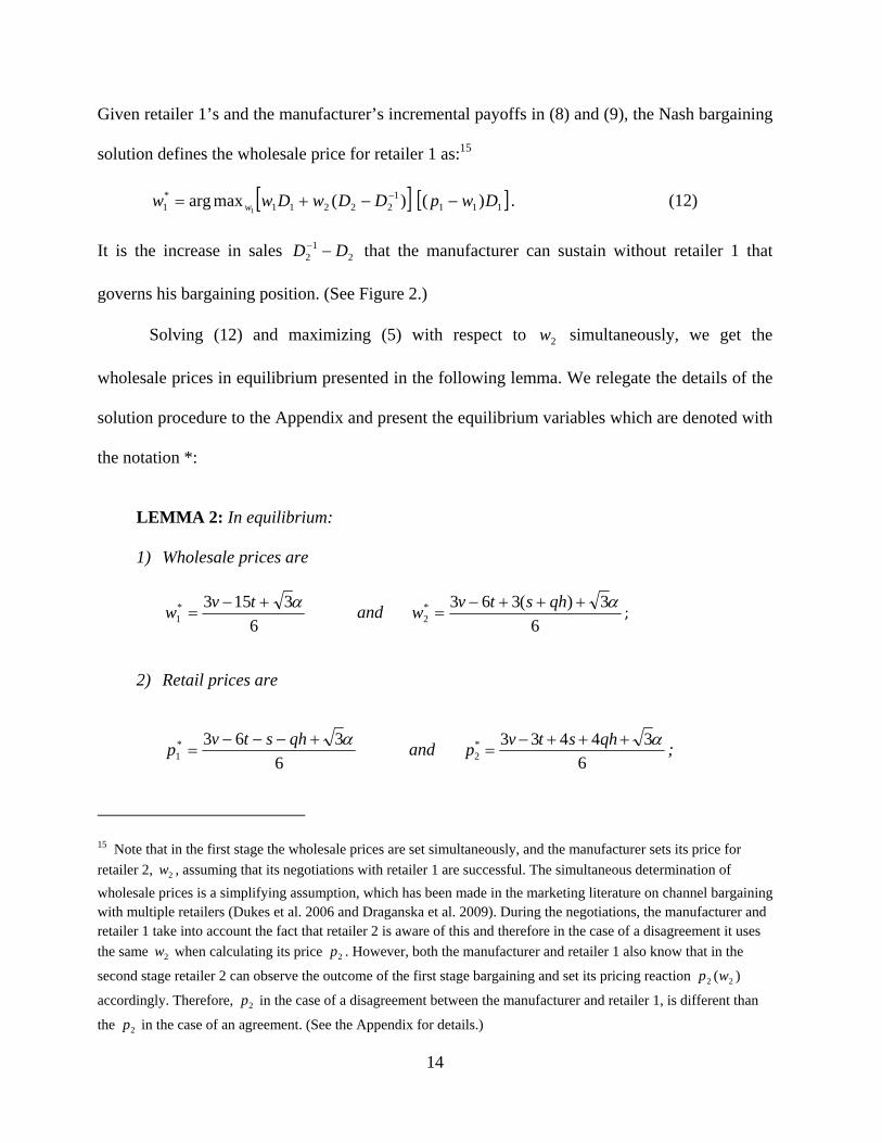
Given retailer 1’s and the manufacturer’s incremental payoffs in (8) and (9), the Nash bargaining
solution defines the wholesale price for retailer 1 as:15
[ ] [ ]1111
22211*1 )()(maxarg
1DwpDDwDww w −−+= − . (12)
It is the increase in sales 21
2 DD −− that the manufacturer can sustain without retailer 1 that
governs his bargaining position. (See Figure 2.)
Solving (12) and maximizing (5) with respect to 2w simultaneously, we get the
wholesale prices in equilibrium presented in the following lemma. We relegate the details of the
solution procedure to the Appendix and present the equilibrium variables which are denoted with
the notation *:
LEMMA 2: In equilibrium:
1) Wholesale prices are
6
3153*1
α+−=
tvw and 6
3)(363*2
α+++−=
qhstvw ;
2) Retail prices are
6
363*1
α+−−−=
qhstvp and 6
34433*2
α+++−=
qhstvp ;
15 Note that in the first stage the wholesale prices are set simultaneously, and the manufacturer sets its price for retailer 2, 2w , assuming that its negotiations with retailer 1 are successful. The simultaneous determination of wholesale prices is a simplifying assumption, which has been made in the marketing literature on channel bargaining with multiple retailers (Dukes et al. 2006 and Draganska et al. 2009). During the negotiations, the manufacturer and retailer 1 take into account the fact that retailer 2 is aware of this and therefore in the case of a disagreement it uses the same 2w when calculating its price 2p . However, both the manufacturer and retailer 1 also know that in the
second stage retailer 2 can observe the outcome of the first stage bargaining and set its pricing reaction )( 22 wp
accordingly. Therefore, 2p in the case of a disagreement between the manufacturer and retailer 1, is different than
the 2p in the case of an agreement. (See the Appendix for details.)

15
3) Retailer and manufacturer profits are:
tqhst
72)9( 2
*1
−−=Π ,
tqhst
72)3( 2
*2
++=Π and
)(24
3451)3(2612 2222* qK
ttttsqhsthqstv
M −+−+++++
=Πα
where )431(3)623(2)2(622 22222 vtvttsvqhtvsshq +−+−++−++≡α .
Figure 2: The Bargaining Position of the Manufacturer when Negotiating with Retailer 1
12−D 2D
12−−++ phqsv
2phqsv −++
Retailer 2
1pv −
Retailer 1
16
Comparing the wholesale prices for retailer 1 in Lemmas 1 and 2, we decompose the
wholesale price paid by retailer 1 into two parts.
PROPOSITION 1: The equilibrium wholesale price can be decomposed as follows:
Δ+′= 1*1 ww , 0>Δ for tv 8> ; and 0/ >∂Δ∂ q .
Proposition 1 decomposes the wholesale price *1w where Δ represents a premium accruing to the
manufacturer because of retailer 2’s gains in sales when, due to disagreement, retailer 1 is
foreclosed from the sale of the manufacturer’s product. These gains ( 021
2 >−− DD ) provide the
manufacturer a better disagreement point when negotiating with retailer 1. Therefore, relative to
the case when 21
2 DD =− the manufacturer can negotiate a higher wholesale price ( 1*1 ww ′> ).
Moreover, the premium Δ increases with quality q because the manufacturer can extract more
surplus from the consumers the higher the quality of the product is ( 0/*2 >∂∂ qw ). Conversely, a
quality reduction improves retailer 1’s relative bargaining position vis-à-vis the manufacturer,
which has a downward effect on the negotiated wholesale price. We call this the “bargaining
position effect” of quality reduction.
2.2 Firms’ Profits and the Quality Decision
Next we examine the effect of product quality on firms’ profits and evaluate the impact of the
distribution of decision rights for quality. We first establish the opposing preferences for quality
through the channel as implied by the equilibrium results of Lemma 2 in the following
proposition.
17
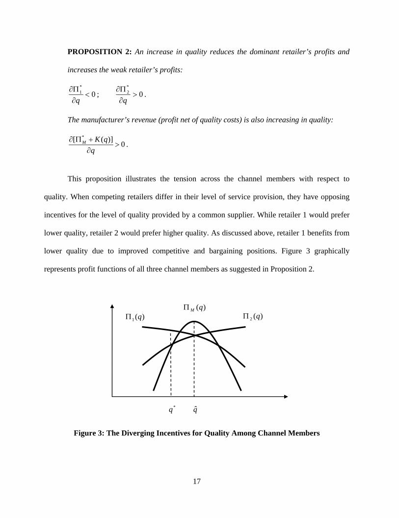
PROPOSITION 2: An increase in quality reduces the dominant retailer’s profits and
increases the weak retailer’s profits:
0*1 <
∂Π∂q
; 0*2 >
∂Π∂q
.
The manufacturer’s revenue (profit net of quality costs) is also increasing in quality:
*[ ( )] 0M K qq
∂ Π +>
∂.
This proposition illustrates the tension across the channel members with respect to
quality. When competing retailers differ in their level of service provision, they have opposing
incentives for the level of quality provided by a common supplier. While retailer 1 would prefer
lower quality, retailer 2 would prefer higher quality. As discussed above, retailer 1 benefits from
lower quality due to improved competitive and bargaining positions. Figure 3 graphically
represents profit functions of all three channel members as suggested in Proposition 2.
q̂
)(1 qΠ )(2 qΠ )(qMΠ
*q
Figure 3: The Diverging Incentives for Quality Among Channel Members

18
The equilibrium level of quality in this asymmetric channel depends on who controls this
decision. If the manufacturer has full control of quality, it will invest in q up to the optimality
condition:16 0/* =∂Π∂ qM . Denote this level of quality as q̂ . However, if retailer 1 has influence
over the level of quality, then it would always induce lower quality qq ˆ< .
To illustrate suppose that the manufacturer and retailer 1 negotiate on the level of quality
before the wholesale prices are set. In this case, the Nash bargaining solution defines a level of
quality q which maximizes the product )~( **1 MM Π−ΠΠ , where MΠ~ is the manufacturer’s profit
in the case of a breakdown in the quality negotiations.17 Denote this negotiated level of quality as
*q . Proposition 3 demonstrates the relationship between *q and q̂ .
PROPOSITION 3: Let the manufacturer’s cost of quality be )(qK be sufficiently
convex to guarantee a unique (finite) level of quality q̂ that maximizes manufacturer’s
profit *MΠ . If *q is the jointly decided level of quality determined through negotiations
between the manufacturer and retailer 1, then *q < q̂ .
The proposition guarantees that any negotiated level of quality will be less than the
manufacturer prefers. In light of shifting channel power, a discount retailer will exert influence
on the quality decision in the direction it prefers, which is downward (Proposition 2). Proposition
16 An interior q̂ that maximizes *MΠ is finite if )(qK is sufficiently convex.
17 We assume that the disagreement payoff to retailer 1 is zero and that the manufacturer can still sell its product through the weak retailer and make a positive profit. For example, with the specification 2)( cqqK = , c sufficiently
large, the manufacturer sets )8/()(~ 2hctvshq −+= , yielding the optimal profit )8/()(~ 22 hctvscM −+=Π .

19
3 confirms that retailer 1 would exert its influence toward lower quality. Furthermore, the
dominant retailer’s influence is to the annoyance of the manufacturer and the rival retailer.18
The model, however, also points to strategies for the weak retailer and the manufacturer
to react against this influence. We interpret these strategies as investments in a service
advantage, which is exclusive to the weak retailer. Specifically, the retailer and manufacturer
may want to engage in joint programs that simultaneously help restore the manufacturer’s
bargaining position and the weak retailer’s competitive advantage.
The model parameters s and h represent the service advantage of retailer 2. As its service
advantage increases, retailer 2 becomes more competitive while this hurts retailer 1
(hshs ∂Π∂
∂Π∂
<<∂Π∂
∂Π∂ *
2*2
*1
*1 ,0, ). However, it is instructive to discuss the effect of these service
parameters on the manufacturer profits. It is clear from the discussion in the previous section that
the manufacturer benefits from strengthening its bargaining position in its negotiations with
retailer 1.
A means by which the manufacturer strengthens its bargaining position is by helping the
rival retailer so that it can provide better service to its customers (Note that 0/,/ ** >∂Π∂∂Π∂ hs MM ).
For example, the manufacturer can offer in-store fixturing and training of the store personnel so
that they know how to position and sell the products.19 Improving store service and design can
18 One can evaluate the impact of the manufacturer’s disagreement payoff MΠ~ on the negotiated level of quality. All
else equal, an increase in MΠ~ gives the manufacturer a stronger say in negotiations over quality and leads to higher
*q . (Formally, qq ˆ* → as *~MM Π↑Π .)
19 An illustration of this practice can be found in the cookware industry, in which manufacturers seek out exclusive partnerships with independent specialty retailers (Gorman 2001).

20
increase the manufacturer’s profits through retailer 2, and therefore, strengthen its bargaining
position vis-à-vis the dominant retailer.
The manufacturer gains because she can negotiate a higher wholesale price 1w . This
bestows an indirect benefit to the weak retailer by relaxing the competitive pressure in retail
prices. The manufacturer gets some additional benefit of relaxed price competition via a higher
wholesale price 2w . Although this raises retailer 2’s costs, the increased demand due to its
service advantage more than compensates its loss due to the higher wholesale price.
3. Implications for Consumers
In this section we investigate the impact of quality reduction on consumer surplus. As mentioned
in the introduction, there are expressed concerns that dominant retailers’ influence on quality
may have detrimental effects on consumers. But our model suggests that the implications of this
influence are not obvious. On one hand, as the quality level of the products sold decreases, the
direct utility that consumers derive from these products should decrease. On the other hand,
prices may fall with lower quality, giving consumers potentially more value. Determining the net
consequence of these two opposing effects is the objective of this section.
Note that one reason prices can fall with lower quality is that lower quality is cheaper to
produce. Benefits to consumers, net of lower utility from quality in this case, would come from
market expansion facilitated by lower prices. However, by construction, in our model marginal
costs and market size are fixed. This permits us to isolate changes to consumer surplus stemming
solely from shifts in rents, rather than from efficiency gains or lower production costs. This is an
important distinction because we are thus able to pinpoint the role that quality plays in the
distribution of market power.

21
Consumer surplus is computed, as a function of quality q and the other variables
associated with quality, s and h, as
∫∫ −−−+++−−=1
20 11
1 ))1(()(D
DdxpxthqsvdxptxvCS . (13)
To assess the impact of quality changes on consumer surplus, we evaluate the sign of the partial
derivatives of equilibrium CS* in the following proposition.
PROPOSITION 4: Let v be as defined in the Appendix.
1) If vv < , then consumer surplus is increasing in q, 0/* >∂∂ qCS ;
2) If vv > , then consumer surplus is decreasing in q, 0/* <∂∂ qCS .
To understand the results of Proposition 4, recall that quality reduction has two opposing
effects on consumer surplus. There is a direct negative effect on consumer utility (See (1)). But
there is also an indirect positive effect through its effect on negotiations and subsequent retail
prices.
To assess which of these two effects is stronger, it is helpful to interpret the conditions
for v that distinguish the two cases. When vv < , quality is an important factor in consumers’
utility. The direct effect on utility from a quality change is stronger than the indirect effect on
paid prices. Therefore, any reduction in manufactured quality q lowers consumer surplus overall.
When v is large, on the other hand, the direct role that quality plays in a consumer’s
utility from consumption is relatively small. Therefore, it is the indirect effect of quality on
prices that is the most important for consumer surplus. Specifically, when quality is reduced, the
manufacturers’ bargaining position is weakened, ensuring a lower wholesale price for retailer 1
and causing a downward effect on both retail prices. Since product quality is less important for
consumers, reducing the quality increases consumer surplus.

22
The above result is noteworthy in light of the popular discussion on retail dominance. It
says that when a discount retailer, retailer 1 in our model, has influence on quality, it may
actually benefit consumers in some cases. Consider products with relatively large v, which one
might interpret as ordinary commodity goods, for example. Retailers who exert their influence
on manufacturer’s production quality serve to reduce retail differentiation and lower the
manufacturer’s market power. This process benefits consumers. We emphasize, however, that
this is not always the case. Indeed, for products with small v, our model suggests the opposite
impact: retailer influence on quality is harmful to consumers.
4. Two Products
While manufacturers often sell the same product to all retailers, there are many instances in
which this is not the case. A manufacturer’s high quality product may be found only at high
service retailers while its lower quality product only at discounters or low service retailers. In
this section we show that the dominant retailer may have an incentive to reduce quality even if
the manufacturer uses a two product strategy.
To see this suppose that products L and H are sold to the end consumers through retailers
1 and 2, respectively. Let LH qq > denote the qualities of the two products offered by the
manufacturer. Accordingly, we modify the consumers’ utility function (1) to:
⎪⎩
⎪⎨
⎧==
−−−++−−++
=otherwise.
;2 if;1 if
0)1()( 222
111
ii
pxtqhsvptxqhsv
xU H
L
i (14)
In order to guarantee that, in the equilibrium of this two product model, the entire market
is covered and each retailer’s demand is positive, we require the following assumption, which is
the two-product analog of Assumption 1.

23
ASSUMPTION 2: vv ˆ> ( v̂ defined in the Appendix) and tqhsqhs LH 5)()( 1122 <+−+ .
We now identify a sufficient condition for which the dominant retailer has the incentive
to exert its influence for lower quality even if the manufacturer has the ability to separate its
products by selling different qualities through the different retailers. The condition requires that
two different quality products manufactured under the same brand are not entirely independent.
Such dependence is implied by the notion that a manufacturer’s brand equity may be negatively
affected if it extends its product line with a lower quality product while retaining the brand name
(Randall et al. 1998). Assuming that brand equity plays a role in consumer’s perception of
product quality, then the perceived quality of the high-end product at the high service retailer
may be adversely affected by the declining quality of the product at the low-service retailer.
To make this precise, suppose that these qualities are represented by an objective quality
component HLjqoj ,, = and a common brand quality component bq , so that bo
jj qqq += . The
objective component represents all aspects of the product that can be measured, such as
durability, product dimensions, or quantifiable performance measures. The brand component
captures the non-objective aspects of quality associated with the brand, such as reputation or
image. Further, assume that this brand component depends on the objective qualities of the two
products: ),( oH
oL
b qqq with 0/),( >∂∂ oj
oH
oL
b qqqq , for j = L,H. The derivative indicates the degree
to which objective quality affects the brand quality. For instance, if this derivative is large, it
means that reducing the quality of the “low end” of the product line can hurt the “high end”.
Under this scenario, a low-service retailer pursuing quality reduction of the product sold in its
store creates a spillover reduction across the remainder of the product line. This opens up the
possibility of restoring the incentive of quality reduction by a low-service retailer even with

24
retailer-specific products. The following proposition states exactly how large this spillover must
be for retailer 1 to benefit from quality reduction.
PROPOSITION 5: If 12
1
hhh
oL
b
−>
∂∂
, then incentive for quality reduction exists, ;0**
1 <∂Π∂
oLq
otherwise 0**
1 ≥∂Π∂
oLq
.
According to the proposition, if retailer 1’s relative ability in highlighting of
quality, )/( 121 hhh − , is low, it benefits from sacrificing its own quality oLq . With inferior
highlighting skills, quality does not help retailer 1 much in extracting surplus from the
consumers. Therefore, a reduction in its quality through its effect on brand reputation helps
retailer 1 by reducing retailer 2’s competitive advantage over retailer 1 (i.e. competitive position
effect) and by improving its relative bargaining position vis-à-vis the manufacturer (i.e.
bargaining position effect).
5. Summary & Conclusion
An important trend in the retailing industry and distribution channel management is the
emergence of dominant retailers such as Wal-Mart. These retailers use their channel power to
influence not only the manufacturers’ wholesale pricing decision but also their choice of product
quality. As a reaction to the growth of the dominant retailers, other retailers try to remain
competitive by improving the design of their stores to highlight their products’ quality attributes
and by their attention to customers.
In this paper we use a model that captures these aspects of the current retailing
environment. Specifically, in our model there are two asymmetric retailers that compete for the
sale of a single product supplied by a common manufacturer. The retailers are asymmetric with

25
respect to the level of their service and their influence on the manufacturer’s choice of quality
and price.
Using such a model, we are able to identify two benefits that accrue to the low service
retailer from a reduction in product quality. First, a quality reduction improves the dominant
retailer’s competitive standing against the other retailer by lessening the importance of quality
for consumer choice. Second, it weakens the manufacturer’s outside option, and therefore
improves the low service retailer’s relative bargaining position.
These benefits come at the expense of the other channel members however. Quality
reduction hurts the high service retailer because it loses demand to the rival retailer. It hurts the
manufacturer because it not only weakens the manufacturer’s relative bargaining position vis-à-
vis the low service retailer but also with a low quality product the manufacturer extracts less
surplus from the consumers. Thus, the channel members have diverging incentives for product
quality. If the low service retailer becomes dominant it may induce a level of quality that is
detrimental for the other members of the channel.
There are also concerns that the dominant retailers’ influence in lowering product quality
is detrimental to consumers. However, we show that this is not necessarily the case because the
price that consumers pay decreases when the manufacturer is weakened in negotiations. As
emphasized, prices will decline with lower quality even though the marginal cost and market size
are constant in quality. Thus, our results show the possibility of a surplus transfer from the firms
to the consumers as a result of a quality reduction.
But what can a manufacturer do when faced with a dominant retailer that uses its channel
power to influence product quality? We show that when faced with such a threat, the
manufacturer can improve its position in the negotiations by helping the rival retailer to improve
26
its service to the customers. With a better outside option, the manufacturer can charge a higher
wholesale price to the dominant retailer.
In addition, the manufacturer may develop channel specific products to mitigate the
spillover effects of quality, for example by selling its lower quality product at the low service
retailer and the high quality product at the high service retailer. Our results show that despite
having retailer specific products, a dominant low-service retailer may still benefit from lower
quality whenever there is a strong common brand component across the manufacturer’s product
line.
Our results may suggest long term product and distribution strategies for manufacturers
which are not modeled here. For example, if manufacturers see quality eroding due to dominant
retailers, then they can consider producing private labels of high quality for traditional retailers.
The advantage of these private labels is that the dominant retailers cannot influence their quality.
Alternatively, the manufacturers may consider withdrawing their high quality brands from the
dominant retailers and distribute only through high service retailers.
The effects of dominant retailers on product specifications and quality are important in
current retailing practices. Further research can study related issues such as how dominant
retailers affect the product line decisions by manufacturers and the implications of supplier
competition on the incentives identified in this paper. We hope our research inspires further
interest in this topic.

27
Appendix
This Appendix contains the proofs of Lemmas 1-2 and Propositions 1-5.
Proof of Lemma 1: Pricing reactions in the second stage, derived from the first order conditions
of the maximization in (3), are given by:
)23(),( 2131
211 qhswwtwwp −−++= (A1)
)23(),( 2131
212 qhswwtwwp ++++= .
The second order conditions for the maximizations of (3) are satisfied because
01)( 2
2
<−=∂
Π∂tpi
i , 2,1=i
Pricing reactions in (A1) are used in the maximizations of (5) and (10) given the demands
in (2) and our assumption that .21
2 DD =− The first order conditions for the maximizations of (5)
and (10) are:
0)(23 21 =−+++ wwtsqh (A2)
0)34()3( 122
21 =−−+−−+−+ sqhtwwwwtsqh (A3)
respectively. Simultaneous solution of (A2) and (A3) provides 1w′ and 2w′ in the lemma. The
second order condition for the maximization of (5) is satisfied since 031
)( 22
2
<−=∂Π∂
twM . The
second order condition for the maximization of the Nash bargaining product (10) evaluated at 1w′
and 2w′ tqhst
wF
108)9(
)(
2
21
2 −−−=
′∂∂ is negative as well.
28
Note that equilibrium retail prices are found by using ),( 21 ww ′′ in (A1) and the optimal
profits by using ),( 21 pp ′′ and ),( 21 ww ′′ in (3) and (5) and that the market is covered since for the
threshold customer )](64512[2)( 61
2111 qhstvppshqvDU ++−=′−′−−+=′
is positive if 4/15tv > , which holds under Assumption 1. Q.E.D.
Proof of Lemma 2: Note that in the maximization (12), the retailers reactions in (A1) are used in
1D and 2D . However, since both the manufacturer and retailer 1 take into account the fact that
once the negotiations are over, retailer 2 knows whether or not they are successful, the 2p used
in 12−D is different. In the case of a disagreement between the manufacturer and retailer 1,
retailer 2 maximizes its profits 12
12
12
−−− =Π pD . This maximization implies
221
2whqsvp +++
=− . (A4)
Using (A4) in (12) implies the following first order condition
02)63(]8)3(5[
4)3()3(
22221
21
2
12 =⎪⎭
⎪⎬⎫
⎪⎩
⎪⎨⎧
−++++−−++
+−+−+−−
wvtqhswwtqhsw
wtqswwsqht
(A5)
Solving (A2) and (A5) simultaneously we get the wholesale prices given in the proposition.20 As
mentioned above, second order condition for the maximization of (5) is satisfied
since: .031
)( 22
2
<−=∂Π∂
twM Denoting the Nash product in (12) by F , we also verify the second
order condition for the maximization at ),( *2
*1 ww : 0
216)3636243()(
)( 2
2
21
2
<−−++
−=∂∂
ttqhstqhs
wF .
20 Notice that the α used in *1w and *
2w is real since >+−+−++−++ )431(3)623(2)2(622 22222 vtvttsvqhtvsshq
0)3()3()3( 222 >−+−+− tvtstqh .

29
Equilibrium retail prices are found by using ),( *2
*1 ww in (A1) and the optimal profits by using
),( *2
*1 pp and ),( *
2*1 ww in (3) and (5).
Note that the market is covered when the negotiations are successful since under
Assumption 1: 0)323336()2()( 121
1221
11 >−+++=−−−++= αtqhsvtppqhsvDU . And
retailer 2 does not sell to the entire market in the case of a breakdown in negotiations since for
the consumer at 0=x under Assumption1: tpqhsvU −−++= −− 12
12 )0(
0)36333(121 <−−++= αtqhsv . This justifies our demand specifications in (2) and (11).
Q.E.D.
Proof of Proposition 1: Using *1w from Lemma 2 and 1w′ from Lemma 1 we get
Δ=+−++=′− )3243(61
1*1 αtqhsvww . (A6)
Thus, Δ is positive for tv 8> .
Taking the derivative of (A6) with respect to q we get
0)6223(3>
−+++=
∂Δ∂
αtqhsvhh
q. (A7)
The derivative in (A7) is positive if tv 2> , which holds under the threshold given for v in
Assumption 1. Q.E.D.
Proof of Proposition 2: Using the equilibrium values in Lemma 2: 036
)9(*1 <
−−−=
∂Π∂
tqhsth
q,
036
)9(*2 >
++=
∂Π∂
tqhsth
q and [ ] 0)3(36)3(34
12)]([ *
>++++−+=∂+Π∂
tqhstvtqhstth
qqKM α
α
for tv 2> , which is implied by the threshold given for v in Assumption 1. Q.E.D.

30
Proof of Proposition 3: Let *q be a maximizer of )~()( **1 MMqG Π−ΠΠ≡ , which uniquely exists
for )(qK sufficiently convex. Then *q must satisfy the first order condition of this maximization:
[ ] ( ) 0~
)(~)(***
***
1**
*1 =
∂Π−Π∂
Π+Π−Π∂Π∂
=∂∂
MMMM
qqqq qqq
qqG .
By Proposition 2 and the fact that 0~)( ** >Π−Π MM q , the first additive term above is negative.
Therefore, the second term is positive. Also observe that
( )⎪⎭
⎪⎬⎫
⎪⎩
⎪⎨⎧
∂Π−Π∂
Π=⎪⎭
⎪⎬⎫
⎪⎩
⎪⎨⎧
∂Π∂
== **
~)(sgnsgn
***
1
*
MM
M
q
since 0)( **1 >Π q and MΠ~ does not depend on q. Hence, )(* qMΠ is increasing in q at *q .
Finally, since 0/ 2*2 <∂Π∂ qM for )(qK sufficiently convex, we can conclude that M’s optimal
quality q̂ must exceed the negotiated quality *q . Q.E.D.
Proof of Proposition 4: Computing the consumer surplus in equilibrium as defined in (13) gives
the expression:t
ttsqhtthqstvCS144
324)15(2813072 2222* α−++++++= . Thus,
hzq
CS=
∂∂ *
, zs
CS=
∂∂ *
, and qzh
CS=
∂∂ *
(A8)
where )72/()]15(336)3(324[ αα ttsqhtvtqhstz +++−−+−= .
Note that hyqv
CS=
∂∂∂ *2
, ysv
CS=
∂∂∂ *2
, and qyhv
CS=
∂∂∂ *2
with )2/(])2(812(3[ 32 αsvvtqhtsty −−+−=
and that 0<y if ,2tv > which holds under Assumption 1. Therefore, the partial derivatives in

31
(A8) are monotonic and decreasing in v. Solving 0=z for v we get
)]}699563(3)283(3642620978433[))]1215720452(2)12015(6)152(2867512430
72030()15[(3{))15(2301071(3
1
2222322333
5.0322322223343
22344422222
tstsqhtshqtsttsshqtsttssqhtstshqtshqtst
tstsshqtsqhtsqhstshqt
v
−+++++−+++
−−++−+++++−
−+++++−−−−
=
Hence, the expressed signs of the derivatives in the proposition depend on the relative order of v
and v . To see that v is real observe that the term within the square root in v
)]1215720452(2)12015(6)152(286751243072030[)15(
322322223343
2234442
tsttssqhtstshqtshqtsttstsshqtsqhm
−−++−+++++−
−++++≡
is positive when 0=t (i.e., 0)( 50 >+== sqhmt ). Notice also that 0)(60 2
0 >+=∂∂
= sqhtm
t
and 0))(405)(4028917(36/)/( 22 >+−+−=∂∂∂∂ qhstsqhtttm under Assumption 1. Therefore
0/ >∂∂ tm for all 0≥t . This implies that 0>m and ensures that ℜ∈v . Furthermore, if
thqs 3<+ then 0>v . Q.E.D.
Proof of Proposition 5: Given any pair of retail prices, consumers maximize their utility in (14),
from which we get the following demand functions:
tpp
tqhsqhsD LH
22)()(
21 121122
1−
++−+
−= ,t
ppt
qhsqhsD HL
22)()(
21 122211
2−
−+−+
−= . (A9)
In the second stage, the maximization of (3) yields the pricing reactions:
))()(23(),( 11222131
211 LH qhsqhswwtwwp +++−++= (A10)
)).()(23(),( 11222131
212 LH qhsqhswwtwwp +−++++=
Second order conditions for this maximization are satisfied because: .01)( 2
2
<−=∂
Π∂tpi
i
In the first stage, using agreement demands (A9), pricing reactions (A10), and
disagreement demand

32
tpqhsv
D H1
22212
−− −++= (A11)
where 2
22212
wqhsvp H +++=− , maximization of (5) with respect to 2w and maximization of
(12) with respect to 1w yield the following equilibrium wholesale prices:
6
3)5(3 11**1
σ+−++=
tshqvw L and
63)2(3 22**
2σ+−++
=tshqvw H (A12)
.)623(2)(222612231293 1221221222122
21
22
221
222 tssvhqsshqhqsssvstsshqhqvtvt HHLHL −+++−+++++−−+−+−≡σ
Note that σ is real since the term within the square root is greater than 22
22
2 )6()6()2( thqtstv H −+−+− ,
which is positive.
Second order condition for the maximization of (5) is satisfied since:
.031
)( 22
2
<−=∂
Π∂tw
M Denoting the Nash product in (12) by F, we verify the second order condition
for the maximization of (12) at the solution at ( **1w , **
2w ):
0216
)])}()[({36)]()[()( 2
11224272
11222
1
2<
+−+−++−+−=
∂∂
tqhsqhsttqhsqhs
wF LHLH
Note that the market is covered if:
012
32)2(3)2(
21)( 2121
12112211 >−+++++
=−−−++++=σthqhqssv
tppqhsqhsvDU HLLH
which implies:
)]()[(5)275(2)73(252547657369ˆ
1122
122122122212
211
22
221
22
LH
HHLHL
qhsqhsttsshqstshqhqssstsstshqhqtvv
+−+−−++−−++++−−−+−
≡>
And retailer 2 does not sell to the entire market in the case of a breakdown in negotiations since
for the consumer at 0=x : 012
36333)0( 221222
12 <
−−++=−−++= −− σthqsvtphqsvU H
H .
33
This justifies the demand specifications (A9) and (A11).
Equilibrium retail prices are found by using (A12) in (A10) and the optimal profits by
using ),( **2
**1 pp and ),( **
2**
1 ww in (3) and (5) with demands defined as in (A9) which yield:
.72
)9( 21122**
1 tqhsqhst LH ++−−
=Π
Using HLjqqq bojj ,, =+= in **
1Π we get:
.72
))(9( 2212211**
1 tsshqhhqhqt o
Hbo
L −+−−++=Π
Then:
⎥⎥⎦
⎤
⎢⎢⎣
⎡
∂
∂−+
−+−−++=
∂
Π∂oL
boH
boL
o qq
hhht
sshqhhqhqtq
)(36
)(9211
212211
1
**1
Notice that 212211 )(9 sshqhhqhqt oH
boL −+−−++ is positive under Assumption 2,
which implies if 12
1
1 hhh
o
b
−>
∂∂
then 0**
1 <∂
Π∂oLq
otherwise .0**
1 ≥∂
Π∂oLq
Q.E.D.
34
References Bianco, A., W. Zellner, B. Diane, M. France, T. Lowry, N. Byrnes, S. Zegel, M. Arndt, R.
Berner, A. Therese. 2003. Is Wal-Mart too powerful? Bus. Week (October 6) 100-110. Boyle, M., E. F. Kratz. 2005. The Wegmans way. Fortune 151(2) 62-68. Chen, Z. 2003. Dominant retailers and the countervailing-power hypothesis. RAND J. Econom.
34(4) 612-625. Choi, C. S. 1991. Price competition in a channel structure with a common retailer. Marketing
Sci. 10(4) 271-296. Consumer Reports. 2002. Where to buy lawn equipment, appliances electronics, hardware,
kitchenware…67(2) 11. Cuneo, A. Z. 2003. Levi’s adds signature. Advertising Age 74(40) 24. Desai, P., O. Koenigsberg, D. Purohit. 2004. Strategic Decentralization and Channel
Coordination. Quantitative Marketing and Economics. 2(1) 5-22. Dobson, P., M. Waterson. 1997. Countervailing power and consumer prices. Economic J.
107(441) 418-430. Dobson, P., M. Waterson. 1999. Retailer power: Recent developments and policy implications.
Economic Policy April 135-156. Draganska, M., S. Villas-Boas, D. Klapper. 2009. A larger slice or a larger pie? An empirical
investigation of bargaining power in the distribution channel. Marketing Sci. forthcoming.
Dukes, A., E. Gal-Or, K. Srinivasan. 2006. Channel bargaining with retailer asymmetry. J.
Marketing Res. 43(1) 84-97. Dukes, A. T. Geylani, K. Srinivasan. 2009. Strategic assortment reduction by a dominant retailer
Marketing Sci. 28(2) 309-319. Fishman, C. 2006. The Wal-Mart Effect. Penguin Press, New York. Gerstner, E., J. D. Hess. 1995. Pull promotions and channel coordination. Marketing Sci. 14(1)
43-60. Geylani, T., A. Dukes, K. Srinivasan. 2007. Strategic manufacturer response to a dominant
retailer. Marketing Sci. 26(2) 164-178. Gorman, L. 2001. Defining your cookware niche. Gourmet Retailer 22(5) 126-130.
35
Hotelling, H. 1929. Stability in competition. Economic J. 39(153) 41-57. Ingene, C., M. Parry. 1995. Channel coordination when retailers compete. Marketing Sci. 14(4)
360-377. Jerath, K., S. Hoch, Z. J. Zhang. 2008. The pursuit of retailing dominance: Market dominance,
channel dominance, or both? Working paper, Tepper School of Business, Carnegie Mellon University, Pittsburgh.
Jeuland, A., S. Shugan. 1983. Managing channel profits. Marketing Sci. 2(3) 239-272. Journal Record. 1991. Customers like Sears service, Wal-Mart prices. (January 15). Lal, R. 1990. Improving channel coordination through franchising. Marketing Sci. 9(4) 299-318. Luo, L., P. Kannan, B. Ratchford. 2007. New product development under channel acceptance.
Marketing Sci 26(2) 149-163. McGuire, T., R. Staelin. 1983. An industry equilibrium analysis of downstream vertical
integration. Marketing Sci. 2(2) 161-190. Moorthy, S. 1987. Managing channel profits: Comment. Marketing Sci. 6(4) 375-379. Purohit, D. 1997. Dual Distribution Channels: Competition between Rental Agencies and
Dealers. Marketing Sci. 16(3) 228-245. Raju, J. S., Z. J. Zhang. 2005. Channel coordination in the presence of a dominant retailer.
Marketing Sci. 24(2) 254-262. Randall, T., K. Ulrich, D. Reibstein. 1998. Brand equity and vertical product line extent.
Marketing Sci. 17(4) 356-379. Trivedi, M. 1998. Distribution channels: An extension of exclusive retailership. Management
Sci. 44(7) 896-909.
Useem, J., J. Schlosser, H. Kim. 2003. One nation under Wal-Mart. Fortune 147(4) 65-78.
Top Related