


Languages
Pages
Legal

AD-768 969
COMPUTATIONAL METHODS FOR ANTENNA PATTERN SYNTHESIS
Joseph R. Mautz, et al
Syracuse University
Prepared for:
Air Force Cambridge Research Laboratories
August 1973
DISTRIBUTED BY:
KTDl National Technical Information Swvict U. S. DEPARTMENT OF COMMERCE 5285 Port Royal Road, Springfield Va. 22151

UNCLASSIFIED
Steurtt» CU««tflc»llon Oh IM flfcg DOCUMENT CONTROL DATA -R&D
(tnurllr tlnttlltult» »I nil; boar «< «HIMCI mt Intntoi mnmlmili) mumi k* mitnd mhjm Wi« tmmll rnttl If tlmttllltäi
Syracuse University Department of Electrical and Computer Engineering Svracu.e. New York TMIO
a«, »tpenj SICUHITV Ck*Miric*TiOM UNCLASSIFIED
I «OaMT TITkC
COMPUTATIONAL METHODS FOR ANTENNA PATTERN SYNTHESIS
ISCniPTIVK NOTC9 (Tfß* *t rmpmt mn4 Intlutln tfaf««) Scientific, Interim
»■ *WTM»J>HI (rim SSm, mi*um iniiiml, JSilmSj
Joseph R. Nautz Roger F. Harrington
• ■ NtPONT OATC
August 1973 7m. TOTAL NO. OF PAGCS
47 Ji. NO. OF RCFI
12 M. CONTN4CT OK 6AANT NO-
F19628-73-C-0047 * PROJtCT. TASK, AND WORK UNIT NO.
5635-06-01 c, 300 ELEMENT
61102F A OOOSUiEUEMENTggj^Qj
M. OniOINATON'S RCFORT NUMRCNIt)
Scientific Report No. 2
•ft. OTHER «roRT HOW (Any olhtl numbmn Oiml mmr ft« •••Ijn»« Ml/a impmtl) r m-
AFCRL-TR-73-0500
10. OKTRISUTION tTATIMCNT
A - Approved for public release; distribution unlimited
M. IUPFLCMCNTANV NOTES
TECH, OTHER
11. »RONSORtNa MILITANT ACTIVITY
Air Force Cambridge Research Laboratories L.G. Hanscom Field (LZ) Bedford, Massachusetts 01730
Some general numerical methods for antenna pattern synthesis, with and without constraints, are developed in this report. Particular cases considered are (1) field pattern specified in amplitude and phase, (2) field pattern specified in amplitude only, (3) these two cases with a constraint on the source norm, and (4) the first two cases with a constraint on the source quality factor. Both the source and the field are discretized at the beginning, and the methods of finite dimensional vector spaces are used for the computations. The theory is general, but is applied only to point sources arbitrarily distributed in a plane, and to pattern synthetsls in this plane. Some numerical examples are given for ten sources approximately equispaced on one-half of an ellipse, with the desired field pattern chosen to be the cosecant $ pattern in the first quadrant.
Ätproduo.'J hy
NATIONAL TECHNICAL INFORMATION SERVICE
U S CJepori- ci t of Commet«, Sunna'...:.! VA 22151
Jl DD ,^.1473 UNCLASSIFIED
Sacurity ClauincftUon*

trcCLASSlFIED itcurtly ClHddcatl cation
KKV «0*01
Antenna synthesis
Constrained source norm
Constrained quality factor
Field magnitude synthesis
Numerical methods
Pattern synthesis
UNCLASSIFIED Stcurlly CUuirication

ABSTRACT
Some general numerical methods for antenna pattern synthesis, with
and without constraints, are developed In this report. Particular cases
considered are (1) field pattern specified In amplitude and phase, (2) field
pattern specified In amplitude only, (3) these two cases with a constraint
on the sourc«! norm, and (4) the first two cases with a constraint on the
source quality factor. Both the source and the field are discretlzed at
the beginning, and the methods of finite dimensional vector spaces are used
for the computations. The theory is general, but is applied only to point
sources arbitrarily distributed in a plane, and to pattern synthesis in this
plane. Some numerical examples are given for ten sources approximately
equispaced on one-half of an ellipse, with the desired field pattern chosen
to be the cosecant ^ pattern in the first quadrant.
in

COMPUTATIONAL METHODS FOR ANTENNA PATTERN SYNTHESIS
ABSTRACT 11
I. INTRODUCTION 1
II. ANTENNA SYSTEMS AND VECTOR SPACES 2
III. PATTERN SYNTHESIS WITH PHASE SPECIFIED 6
IV. FIELD MAGNITUDE PATTERN SYNTHESIS 16
V. PATTERN SYNTHESIS WITH CONSTRAINED SOURCE NORM 23
VI. PATTERN SYNTHESIS WITH CONSTRAINED QUALITY FACTOR 30
VII. DISCUSSION 36
APPENDIX - ALTERNATIVE METHOD FOR FIELD liAGNITUDE PATTERN SYNTHESIS 41
REFERENCES 42
Preceding page biafik
I. IMTRODUCTION
The purpose of this report Is to develop some general numerical methods
for the problem of antenna pattern synthesis, with and without constraints.
The principles of pattern synthesis are well known, and many specific problems
have been considered [1]. A good discussion of the general theory and of the
difficulties encountered has been given by Deschamps and Cabayan [2]. To over-
come problems concerning the stability and sensitivity of the solution, they
propose to use regularlzation methods [3], In Hilbert space, this method Is
equivalent to obtaining a least-equares solution with a constraint on the
source norm [4,5]. It Is closely related to obtaining a least-squares solution
with a constraint on the quality factor, as considered in Section VI of this
report.
Most of the methods developed for pattern synthesis assume that the
radiation field is specified in both magnitude and phase. In many cases only
the magnitude is of interest, and the phase is left unspecified. This is a
special case of the so-called mixed problems of antenna synthesis, considered
by Bakhrakh and Troytskiy [6]. An application of field magnitude pattern
[1] For example, see R. E. Collin and F. J. Zucker, "Antenna Theory," Part 1, McGraw-Hill Book Co., New York, 1969, Chap. 7.
[2] G. A. Deschamps and H. S. Cabayan, "Antenna Synthesis and Solution of Inverse Problems by Regularlzation Methods," IEEE Trans., vol. AP-20, No. 3, May 1972, pp. 268-274.
[3] A. N. Tihonov, "Solution of Incorrectly Formulated Problems and the Regularlzation Method," Soviet Mathematics, vol. 4, July-December 1963, pp. 1035-1038.
[4] V. I. Popovkln and V. I. Yelumeyev, "Optimization and Systematization of Solutions to Antenna Synthesis Problems," Radio Engineering and Electronic Physics, vol. 13, No. 5, 1968, pp. 682-686.
[5] V. I. Popovkln, G. I. Shcherbakov, V. I. Yelumeyev, "Optimum Solutions of Problems in Antenna Synthesis Theory," Radio Engineering and Electronic Physics, vol. 14, No. 7, 1969, pp. 1025-1030.
[6] L. D. Bakhrakh and V. I. Troytskiy, "Mixed Problems of Antenna Synthesis," Radio Engineering and Electronic Physics, vol. 12, No. 3, Karch 1967, pp. 404-414.

synthesis to s specific problem hss been published by Chonl [7]. In Section IV
we give a discussion of field magnitude pattern synthesis In terms of numerical
methods.
The procedures developed In this report are general, being applicable to
any antenna system which can be accurately analyzed. However, to keep the
examples and computer programs simple, the theory Is applied explicitly only
to point sources arbitrarily distributed In a plane, and to pattern synthesis
in this plane. The extension to arbitrary N-port systems In three-dimensional
space, and to pattern synthesis over r.he entire radiation sphere, is straight-
forward but tedious In detail. A special case of three-dimensional field magni-
tude pattern synthesis applied to wire scatterers is given in reference [8].
II. ANTENNA SYSTEMS AND VECTOR SPACES
The general relationship between the source f of a radiating system and
the field g it produces on the radiation sphere can be symbolized by
Tf ■ g (1)
where T is a linear operator. In general, both f and g may be infinite
dimensional and T may not be bounded. The pattern synthesis problem can be
summarized as follows: Given a desired field g (specified completely or
partially), we wish to determine a source f (constrained or unconstrained)
whose field g approximates g in some acceptable manner. The approach taken
by Deschamps and Cabayan [2] is to treat the problem In general in function
spaces, and then numerically evaluate the final formulas for specific appli-
cations. Our approach is to discretize the problem at the beginning, and then
treat the problem in finite-dimensional vector spaces.
[7] Y. I. Chonl, "Synthesis of an Antenna According to a Given Amplitude Radiation Pattern," Radio Engineering and Electronic Physics, vol. 16, No. 5, May 1971, pp. 770-778.
[8] R, F. Harrington and J. R. Mautz, "Synthesis of Loaded N-port Scatterers," AFCRL-72-0665, Scientific Report No. 17 on Contract No. F19628-68-C-0180 between Syracuse University and Air Force Cambridge Research Laboratories, October 1972.
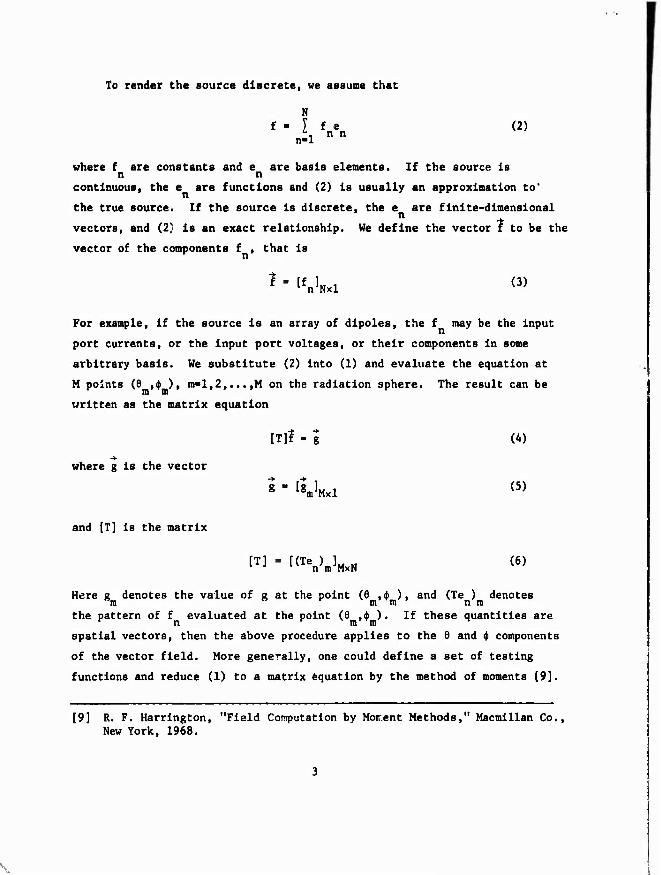
To render the source discrete, we assume that
N f " I fnen (2)
n-1 nn
where f are constants and e are basis elements. If the source Is n n
continuous, the e are functions and (2) Is usually an approximation to' n
the true source. If the source Is discrete, the e are flnlte-dlmenslonal n ^
vectors, and (2) Is an exact relationship. We define the vector f to be the
vector of the components f , that Is
? " IfnW <3>
For example, If the source Is an array of dlpoles, the f may be the Input
port currents, or the Input port voltages, or their components In some
arbitrary basis. We substitute (2) Into (1) and evaluate the equation at
M points (6 ,$ ), m>l,2,...,M on the radiation sphere. The result can be
written as the matrix equation
[T]l - g (4)
where g Is the vector
and [T] Is the matrix
* ■ I*mW (5)
™ • f(Ten)m]MxN (6)
Here g denotes the value of g at the point (6 ,6 ), and (Te ) denotes m m m n m the pattern of f evaluated at the point (6 ,$ ). If these quantities are n mm spatial vectors, then the above procedure applies to the 6 and $ components
of the vector field. More generally, one could define a set of testing
functions and reduce (1) to a matrix equation by the method of moments [9].
[9] R. F. Harrington, "Field Computation by Moment Methods," Macmlllan Co., New York, 1968.

The synthesis problem can now be represented by
ml«g0 (7)
where g is the specified pattern vector. Equation (7) Is a matrix equa-
tion, and the well-known methods of matrix algebra can now be brought to
bear on the problem. If [T] is square and nonslngular, the solution is
given by the inverse to (7). This solution will give the correct value of
field at the M points (6 ,$ ) on the radiation sphere, but no control of m m the field is obtained between these points. If [T] is of rank less than N,
the problem is underdetermlned and more than one solution to (7) exists. In
this case additional constraints can be applied to either the source or the
field to obtain the most desirable solution. If [T] is of rank greater than
N, then usually no exact solution to (7) exists, but there will be a uniaue
least-squares solution. Again additional constraints can hz applied to ob-
tain more desirable solutions.
Let us next define the Euclidean spaces involved more precisely. For
source quantities, the inner product is defined as
<f*, fj* - f^Vjlj (8)
where the tilde denotes transpose, the asterisk denotes complex conjugate,
and [V] is a weight matrix. [V] must be positive definite, and for this
report we consider it to be the diagonal matrix
W • fdla* Vn]NxN (9)
with all v > 0. In the source space the norm induced by the Inner pro-
duct is
||?|| - <f*.f>1/2 - ( f vn|fn|2)1/2 (10) n"l
where f are the components of f. The metric induced by the norm is
d(t. ,t ) ■ llfj - ?. || • For field quantities we define the inner pro-
duct as

<g1.gj> - ^[Wlgj (11)
where [W] Is a weight matrix. It must be positive definite and for this
report we take it to be the diagonal matrix
[W] - [diag wj^ (12)
with all w > 0. In the field space the torm Induced by the inner pro- m duct is
||g|| - <g*.g>1/2 - (f wjgj2)1/2 (13) m"l
whftre g, -re the components of g. The metric Induced by the norm is
dCg^g.) - llgj-gj.
To compare various pattern synthesis procedures, we define two
figures of merit. The first is the normalized synthesis error
M
\t.t II 2 ^ Wn.l8ra-8„m|2
E ^--^ (14) l|g0ll I w |g |2
'', m ' om1 m-l
where g is the synthesized pattern and g is the desired pattern. The
second is the quality factor [10]
N I v |f |2
Q.MJJL2.M4L_UL_ (15) llgll2 fw|g|2
m-l
The multiplier M is introduced Into (15) to make the Q relatively in-
sensitive to the number of field points chosen.
[10] Y. T. Lo, S. W. Lee, and Q. H. Lee, "Optimization of Directivity and Signal-to-Noise Ratio of an Arbitrary Antenna Array, " Proc. IEEE, vol. 54. AuRuat 1966, pp. 1033-1045.
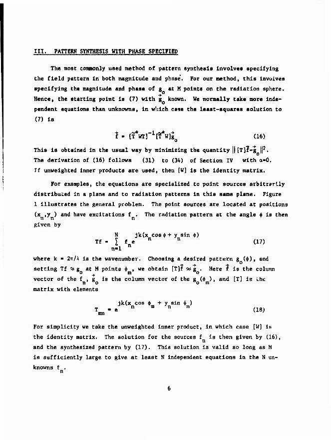
III. PATTERN SYNTHESIS WITH PHASE SPECIFIED
The most commonly used method of pattern synthesis Involves specifying
the field pattern In both magnitude and phase. For our method, this Involves
specifying the magnitude and phase of g at N points on the radiation sphere.
Hence, the starting point is (7) with g known. We normally take more inde-
pendent equations than unknowns, in which case the least-squares solution to
(7) is
I - [TVT]"1^]^ (16)
This is obtained in the usual way by minimizing the quantity || [T]f-g |P.
The derivation of (16) follows (31) to (34) of Section IV with o-O.
Tf unweighted inner products are used, then [W] is the Identity matrix.
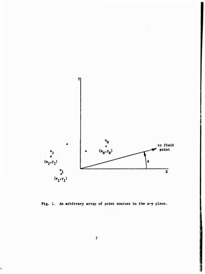
For examples, the equations are specialized to point sources arbitrarily
distributed In a plane and to radiation patterns in this same plane. Figure
1 Illustrates the general problem. The point sources are located at positions
(x ,y ) and have excitations f . The radiation pattern at the angle $ is then
given by
N Jk(x cos ♦ + y sin $) Tf - I f e n n (17)
n-1 n
where k » 2ir/X is the wavenumber. Choosing a desired pattern g ($), and
setting Tf % g at M points <j> , we obtain [T]f *« g . Here f is the column
vector of the f , g is the column vector of the g (^ ), and [T] is the no o m matrix with elements
Jk(x cos $ + y sin $ ) T - e n "' n m (18) mn
For simplicity we take the unweighted inner product, in which case [W] Is
the identity matrix. The solution for the sources f is then given by (16),
and the synthesized pattern by (17). This solution Is valid so long as M
is sufficiently large to give at least N Independent equations in the N un-
knowns t .
(Xj»^
to field point
Cxj^yp
Fig. 1. An arbitrary array of point sources In the x-y plane.

For some numerical results, consider 10 sources approximately
equispaced on one-half of a 2:1 ellipse, as shown in Fig. 2a. For the
radiation pattern, take a rectangle in the first quadrant of the polar
pattern. (This is the so-called cosecant ^ pattern.) 36 field points
i are chosen every 10s in ^, starting at $ •• 5s. These are shown by m crosses on Fig. 2b. For the synthesis we take four cases: (a) origit)
at the center of the ellipse and the field real, (b) origin one-half
the distance from the center to the end point of the semlmajor axis and
the field real, (c) origin at the end point of the semlmajor axis and the
field real, and (d) origin at the center of the ellipse and the field phase
alternating from 0 to 180s between adjacent field points. (This last case
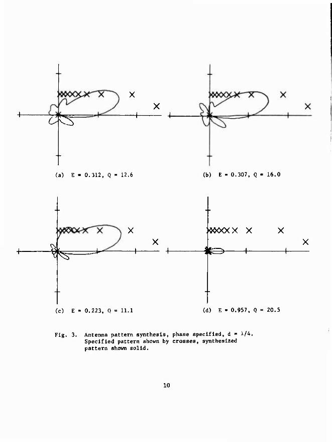
represents the worst choice that can be made.) Figure 3 shows the results
when the sources are separated d - X/A, Fig. 4 when d • X/2, and Fig. 5 when
d =» A, The corresponding normalized synthesis errors E and quality factors 0
associated with each synthesis result are given below each pattern. The
source excitations are listed by magnitude and phase (in degrees) in Tables 1
to 3, normalized so that the maximum excitation is unity.
Some general observations are as follows: When the field Is chosen to
have alternating phase between adjacent points (cases d), the pattern syn-
thesis is poor In each case. When the field Is chosen to he in phase at all
points, with respect to a coordinate origin in the vicinity of the sources,
the synthesis is good when the sources are separated by d » X/4 and A/2, and
poor when separated by d - A. The Q is low when the sources are separated by
d - A/2 and A, but relatively high when d - A/4. These properties are in agree-
ment with what we would expect based on past experience with antenna synthesis
problems.

(a) Source distribution
0<VX)< K—*-
(b) Dealred pattern
Fig. 2. Source distribution and desired pattern for numerical example.
X
c^
(a) E - 0.312, Q - 12.6
X
(b) E - 0.307, Q - 16.0
% ■^r-
X
(c) E » 0.223, Q = 11.1
X «XXXX X
\%=}—h-
(d) E - 0,957, Q - 20.5
Fig. 3. Antenna pattern synthesis, phase specified, d » \lk. Specified pattern shown by crosses, synthesized pattern shown solid.
10

«00O< X X
(a) E - 0.494, Q - 1.86
X X X
^fr3
(b) E - 0.495, Q - 1.70
:s§^<xx
^3^-^
(c) E - 0.438, Q - 1.06
X ;«oo<x x x
(d) E - 0.956, Q - 1.40
Fig. 4. Antenna pattern synthesis, phase specified, d - X/2. Specified pattern shown by crosses, synthesized pattern shown solid.
11

X X
H f
(a) E - 0.748, Q - 1.49 (b) E - 0.691, Q - 1.58
«XXXX X
(c) E • 0.681, Q - 1.27
X «CXXX X X
(d) E - 0.872, Q - 0.889
Flg. S. Antenna pattern synthesis, phase specified, d - X. Specified pattern shown by crosses, synthesized pattern „shown solid.
12
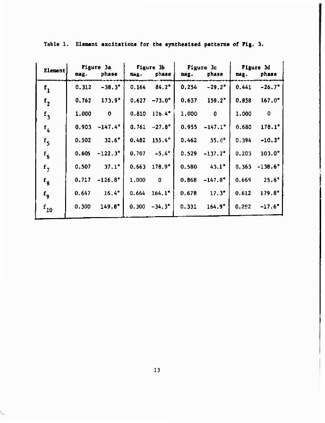
Table 1. Element excitations for the synthesized patterns of Fig. 3.
Element mag. re 3a
phase Flgu
«u.g. re 3b
phase Figure 3c
mag. phase Figure 3d 1
mag. phase
fl 0.312 -38.3, 0.164 84.2° 0.254 -29.2° 0.441 -26.7° |
f2 0.762 173.9° 0.627 -73.0° 0.657 159.2° 0.858 167.0°
f3 1.000 0 0.810 126.4° 1.000 0 1.000 0
fA 0.903 -U7.A0 0.761 -27.8° 0.955 -147.1° 0.680 178.1°
1 f5 0.502 32.6° 0.482 155.4° 0.462 55.0° 0.394 -10.3°
1 f6 0.605 -122.3° 0.707 -5.4° 0.529 -137.2° 0.203 103.0°
f7 0.507 37.1° 0.663 178.9° 0.580 43.1° 0.363 -138.6°
1 f8 0.717 -126.8° 1.000 0 0.868 -147.8° 0.669 25.6°
f9 0.647 16.4° 0.664 164.1° 0.678 17.3' 0.612 179.8°
1 fio 1 0.300 149.8° 0.300 -34.3° 0.331 164.9° 0.292 -17.6"
13
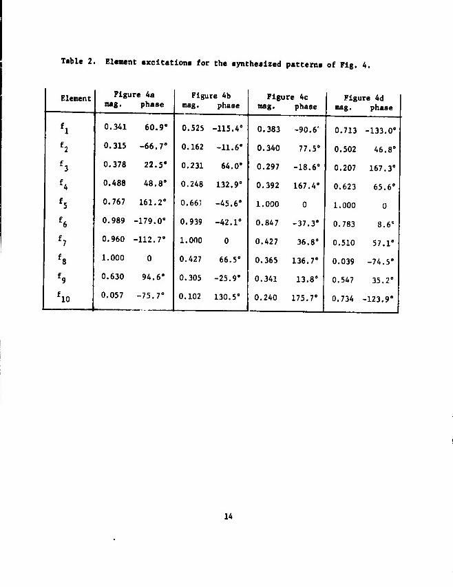
Table 2. Element excitations for the synthesized patterns of Pig. 4.
Element Figure 4a mag. phase
l10
0,341 60.9°
0.315 -66.7°
0.378 22.5*
0.488 48.8°
0.767 161.2°
0.989 -179.0°
0.960 -112.7°
1.000 0
0.630 94.6°
0.057 -75.7°
Figure 4b mag. phase
0.525 -115.4°
0.162 -11.6°
0.231 64.0°
0.248 132.9°
0.66.1 -45.6°
0.939 -42.1°
1.000 0
0.427 66.5°
0.305 -25.9°
0.102 130.5°
Figure 4c mag. phase
0.383 -90.6'
0.340 77.5°
0.297 -18.6°
0.392 167.4°
1.000 0
0.847 -37.3°
0.427 36.8°
0.365 136.7°
0.341 13.8°
0.240 175.7°
Figure 4(1 mag. phase
0.713 -133.0°
0.502 46.8°
0.207 167.3°
0.623 65.6°
1.000 0
0.783 8.6°
0.510 57.1°
0.039 -74.5°
0.547 35.2°
0.734 -123.9°
14
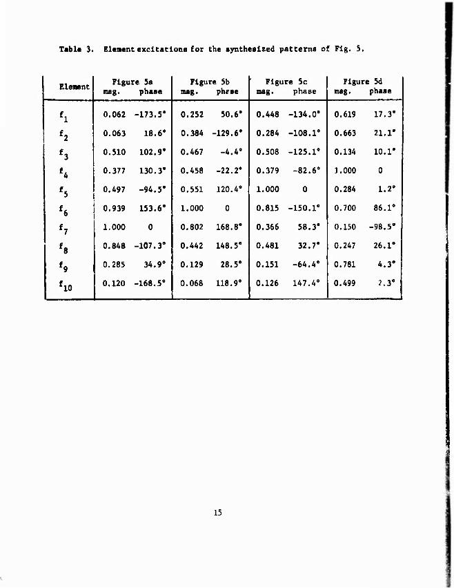
Table 3. Element excitations for the synthesized patterns of Fig. 5.
Element Figure 5a
mag. phase Figure 5b
mag. phese Figure 5c
mag. phase Figure 5d 1
mag. phase 1
0.062 -173.5° 0.252 50.6° 0.448 -134.0° 0.619 17.3°
0.063 18.6, 0.384 -129.6° 0.284 -108.1° 0.663 21.1°
0.510 102.9° 0.467 -4.4° 0.508 -125.1° 0.134 10.1°
0.377 130.3° 0.458 -22.2° 0.379 -82.6° 1.000 0 |
0.497 -94.5° 0.551 120.4° 1.000 0 0.284 1.2°
0.939 153.6° 1.000 o 0.815 -150.1° 0.700 86.1°
1,000 0 0.802 168.8° 0.366 58.3° 0.150 -98.5°
0.848 -107.3° 0.442 148.5° 0.481 32.7° 0.247 26.1°
0.285 34.9° 0.129 28.5° 0.151 -64.4° 0.781 4.3°
f10 0.120 -168.5° 0.068 118.9° 0.126 147.4° 0.499 2.3°
15

IV. FIELD MAGNITUDE PATTERN SYNTHESIS
We next consider the problem of synthesizing a pattern in magnitude
only. Let h <■ |g | be a desired field magnitude, and form the vector h by
specifying its value h at M points on the radiation sphere. Again we con- m *
aider the source to be discretized and represented by the vector f. It is
desired to find the source f for which the pattern error
e - || |[T]I| -S|P (19)
is minimum. In terms of components, (19) becomes
M , N ,2 E "I will f T J -hi (20)
, ml, n mn ml m-1 n-1
where the w are weight factors. To circumvent the troublesome inner m magnitude operation In (20), we first consider the more general function
M . N jß ,2
'$& " ^ wm I I Vmn " V 1 <21) m"l n-1
This Is the error function used when the pattern is specified in both magnitude
h and In phase 0 . Hence, for 6 fixed, the f for minimum e are given by m r M ' m n o / (16). For f fixed, the minimum c Is obtained when both terms within the mag-
nitude signs of (21) are in phase, that is, when
N
Jßn, n-1 fnTlnn
e »--JL-i (22)
I I f T | n-l nmn
Because (21) is more general that (20), Its minimum is less than or equal to
that of (20). But under condition (22), the e of (21) is equal to that of
(20). Therefore (20) and (21) have the same minimum.
16

An iterative procedure for minimizing (21) proceeds as follows:
1. Assume starting values for $., &.,..., ß...
2. Keep the 8 fixed and calculate the f which minimize e using (16). m n
3. Keep the f fixed and calculate the 8 which minimize e using (22). n m
4. Go to step 2.
This procedure eventually converges because steps 2 and 3 cannot increase e.
While the procedure obtains absolute minima in the f space and in the ß space,
it does not necessarily obtain the absolute minimum in the catenated space
(r,ß). Hence, the procedure converges to a stationary point, usually a local
minimum, which may or may not be the global minimum. An alternative procedure
for minimizing (21) is given in the Appendix.
For numerical results, we consider the same example as used in the pre-
ceding section. Hence, the array is illustrated by Fig. 2a, and the radiation
pattern by Fig. 2b. The same three cases of element separation, d - X/4, X/2,
and A, are used. Two starting points were chosen for the iterative procedure:
(a) origin at the end point of the semimajor axis and the field real, and (b)
origin at the center of the ellipse and the field phase alternating between 0
and 180° between adjacent field points. These starting points correspond to
cases (c) and (d) of the previous section. The final results of the magnitude
synthesis procedure are shown in Fig. 6 for d « X/4, Fig. 7 for d » X/2, and
Fig. 8 for d « X, The normalized synthesis errors E and quality factors Q for
each result are given below each pattern. The source excitations are listed
by magnitude and phase in Table 4, normalized so that the maximum excitation
is unity.
17
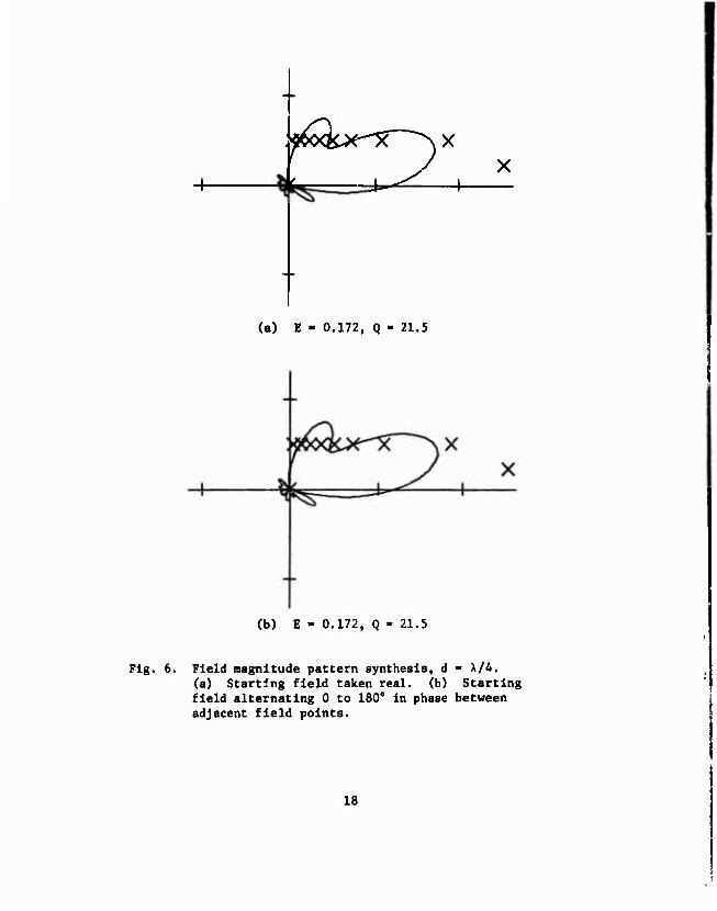
.^OQCX^X "NX
(a) E - 0.172, Q - 21.5
(b) E - 0.172, Q - 21.5
Fig. 6. Field magnitude pattern synthesis, d - X/4. (a) Starting field taken real, (b) Starting field alternating 0 to 180° in phase between adjacent field points.
18
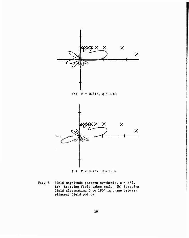
^
ö^X^X X X
(a) E » 0.416, Q « 1.63
EX X X
—4^ 1
(b) E - 0.425, Q = 1.09
Fig. 7, #leld magnitude pattern synthesis, d - A/2. (a) Starting field taken real, (b) Starting field alternating 0 to 180° in phase between adjacent field points.
19
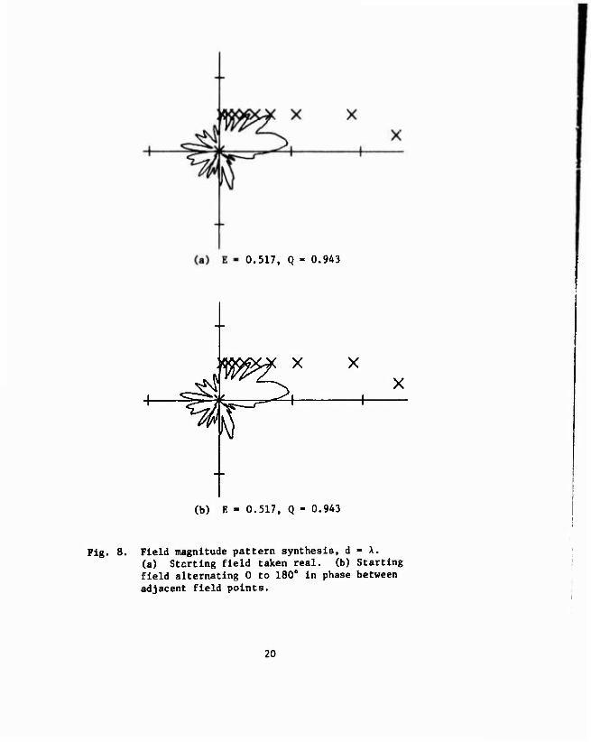
0.517, Q - 0.943
J^ X X
^r" X
(b) E - 0.517, Q - 0.943
Fig. 8. Field magnitude pattern synthesis, d - X. (a) Starting field taken real, (b) Starting field alternating 0 to ISO" in phase between adjacent field points.
20

Table 4. Element excitations for the synthesized patterns of Figs. 6, 7, 8.
1 Ele- ment
Figure 6a mag. phase
Figure 6b mag. phase
Figure 7a mag. phase
Figure 7b mag. phase
Figure 8a mag. phase
Figure 8b j mag. phase
fl 0.264 125.0 0.264 125.0 0.299 -89.5 0.178 -62.0 0.461 -118.7 0.462 -118.8
r 0.626 -40.5 0.626 -40.5 0.362 75.4 0.337 71.2 0.552 -313.2 0.552 -113.1
e 0.985 153.2 0.985 153.2 0.334 -22.9 0.473 -76.9 0.680 -92.7 0.680 -92.8
£4 1.000 0.0 1.000 0.0 0.285 -177,4 0.440 -78.5 0.970 -66.3 0.969 -66.2
f5 0.636 -159.1 0.636 -159.2 1.000 0.0 1.000 0.0 1.000 0.0 1.000 0.0
£6 0.553 24.7 0.553 24.7 0.827 -34.7 0.621 8.0 0.370 -66.4 0.366 -66.4
f7 0.570 -160.3 0.570 -160.3 0.365 51.2 0.832 113.8 0.208 152.2 0.204 152.3
f8 0.664 10.3 0.664 10.3 0.364 151.9 0.698 -154.1 0.371 75.3 0.368 75.3
f9 0.527 172.9 0.528 172.9 0.378 12.0 0.639 -15.2 0.334 -74.7 0.334 -75.2
f10 0.234 -42.8 0.235 -42.8 0.360 161.5 0.643 136.4 0.406 150.0 0.407 150.3
21
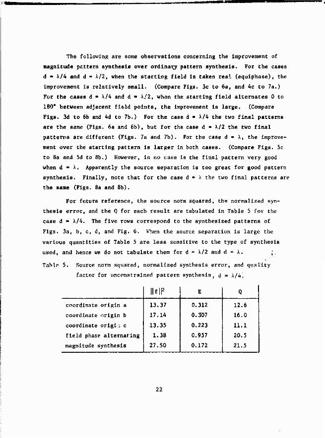
The following are some observations concerning the improvement of
magnitude pcttern synthesis over ordinary pattern synthesis. For the cases
d - A/4 and d ■ X/2, when the starting field is taken real (equiphase), the
Improvement is relatively small. (Compare Figs. 3c to 6a, and Ac to 7a.)
For the cases d - X/4 and d • A/2, when the starting field alternates 0 to
180° between adjacent field points, the Improvement is large. (Compare
Figs. 3d to 6b and 4d to 7b.) For the case d - A/4 the two final patterns
are the same (Figs. 6a and 6b), but for the case d - A/2 the two final
patterns are different (Figs. 7a and 7b). For the case d - A, the improve-
ment over the starting pattern is larger in both cases. (Compare Figs. 5c
to 8a and 5d to 8b.) However, in no case is the final pattern very good
when d = A, Apparently the source separation Is too great for good pattern
synthesis. Finally, note that for the case d = A the two final patterns are
the same (Figs, 8a and 8b).
For future reference, the source norm squared, the normalized syn-
thesis error, and the Q for each result are tabulated In Table 5 for the
case d ■ A/4. The five rows correspond to the synthesized patterns of
Figs. 3a, b, c, d, and Fig, 6. When the source separation is large the
various quantities of Table 5 are less sensitive to the type of synthesis
used, and hence we do not tabulate them for d = A/2 and d «= A. ;.
Tablo 5. Source norm squared, normalized synthesis error, and quslity
factor for unconstrained pattern synthesis, d = A/4.
llfll2 E Q
coordinate origin a 13.37 0.312 12.6
coordinate origin b 17.14 0.307 16.0
coordinate origi : c 13.35 0.223 11.1
field phase alternating 1.38 0.957 20.5
magnitude synthesis 27.50 0.172 21.5
22

V. PATTERN SYNTHESIS WITH CONSTRAINED SOURCE NORM
The source norm is closely related to near-field quantities,
such as power losses in an antenna structure or energy storage. For this
reason It Is often desirable to limit the source norm, especially when the
sources are close together or continuously distributed. Hence, we consider
the problem of minimizing
llm?-gj2 (23) o
subject to the constraint
< C (24)
where C Is a positive constant to be chosen. This constrained minimi-
zation can be accomplished by forming the Lagrangian
J - II [T]l -ijl2 + a ||l||2 (25)
where a is a Lagrange multiplier. If we can obtain the source function f
which minimizes .1 vilh respect to f and are able to find a > 0 such t'iat
l|fi|2=C (26)
then any other source function which satisfies the constraint (2A) gives
at least as large a J and thus at least as large an e as that provided
by f. Hence r minimizes e subjec to the constraint (24).
However, it is not always possible to find a > 0 such that the
f which minimizes J satisfies (26). This warrants an investigation into
the behavior of ||f||2and e attained by the minimizing function f versus
a. If f is the minimizing function when a = a. and f„ is the minimizing
function when a = a., then
23
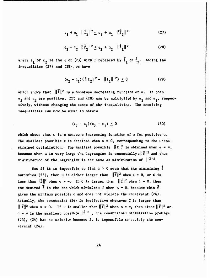
e, + \ ll^ll2ie2 + a1 ||12r (27) 1 ' "l " 'I11 - '2
e2 + a2 ||t2P<e1 + a2 H^P (28)
where e. or e„ is the e of (23) with f replaced by f. or t.. Adding the
inequalities (27) and (28), we have
(a2-al)(||£2li2- HfJI 2) < 0 (29)
which shows that ||f IP is a monotone decreasing function of a. If both
a^ and o. are positive, (27) and (28) can be multiplied by a« and a , respec-
tively, without changing the sense of the inequalities. The resulting
inequalities can now be added to obtain
(a2 " al)(E2 - £l) -0 <30)
which shows that e is a monotone Increasing function of a for positive a.
The smallest possible e is obtained when a = 0, corresponding to the uncon-
strained optimization. The smallest possible ||f|[2 Is obtained when a = «>,
because when u Is very large the Lagranglan is essentially a {{f{|2 and thus
minimization of the Lagranglan is the same as minimization of ||f ||2.
Now if it is Impossible to find a > 0 such that the minimizing f
satisfies (26), then C Is either larger than ||f ||2 when a = 0, or C is
less than ||f ||2 when o » ">. If C is larger than ||f||2 when 0 = 0, then
the desired f is the one which minimizes J when a • 0, because this f
gives the minimum possible c and does not violate the constraint (24).
Actually, the constraint (2A) is ineffective whenever C is larger than
|| f ||2 when a = 0. If C is smaller than ||?||2 when a ■ °», then since ||1||2 at
a ° <» is the smallest possible ||r||2 , the constrained minimization problem
(23), (24) has no solution because it is impossible to satisfy the con-
straint (24).
24
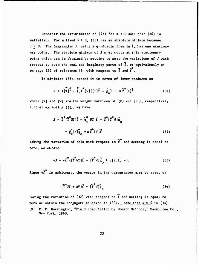
Consider Che minimization of (25) for a > 0 such that (26) is
satisfied. For a fixed a > 0, (25) has an absolute minimum because
J ^ 0. The Lagrangian J, being a qr.adratic form in t, has one station-
ary point. The absolute minimum of J tkiist occur at this stationary
point which can be obtained by setting to zero the variations of J with
respect to both the real and imaginary parts of f, or equivalently as
on page 192 of reference [9j with respect to f and f ,
To minimize (25), expand It in terms of inner products as
J - ("Sr-'g „MWluTll - g ) + at ml (31)
where [V] and [W] are the weight matrices of (8) and (11), respectively.
Further expanding (31), we have
J = f [T WT]f - g fWT]f - f [T W]g
+ g*IW]go +af*[V]f (32)
»V* Taking the variation of this with respect to f and setting it equal to
zero, we obtain
6J - 6f*([T*WT]l - [T*W]g + a[V]f) - 0 (33)
Since 6f Is arbitrary, the vector in the parentheses muse be zero, or
[T WT + aV]f - [T W]g (34)
Taking the variation of (32) with respect to f and setting it equal to
zero we obtain the conjugate equation to (33). Note that a " 0 in (34)
[9] R. F. Harrington, "Field Computation by Moment Methods," Macmlllan Co., New York, 1968.
25
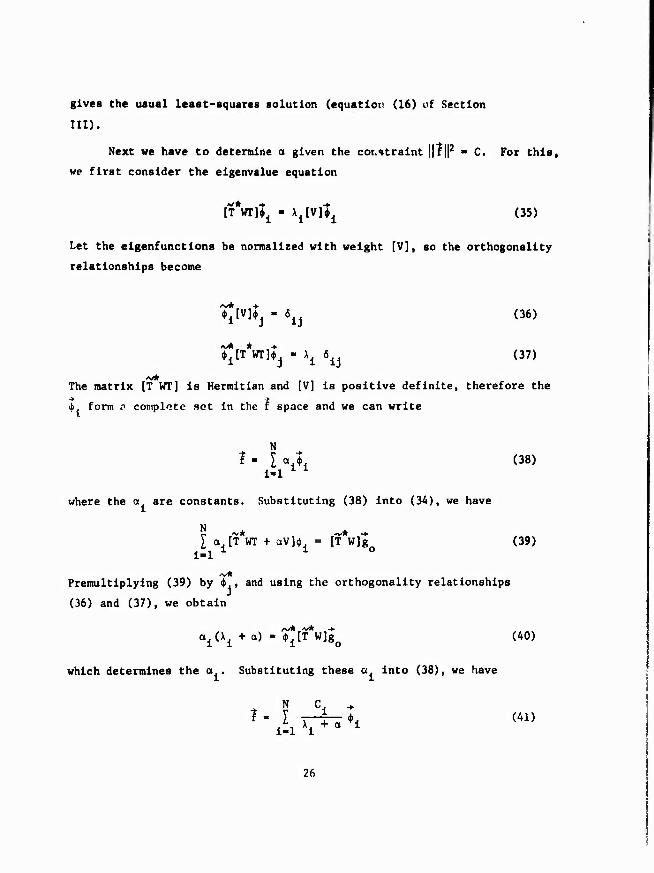
gives the usual least-squares solution (equation (16) of Section
III).
Next we have to determine a given the constraint ||t||2 - C. For this,
we first consider the eigenvalue equation
[T OTjIj - ^[V]^ (35)
Let the eigenfunctions be normalized with weight [V], so the orthogonality
relationships become
♦JlVllj - 6 (36)
^lT*WTl| - X1 6^ (37)
AM The matrix [T WT] is Hermitian and [V] is positive definite, therefore the
4 form <-> complete set in the f space and we can write
I ■ I CLI (38) 1-1
where the a are constants. Substituting (38) into (34), we have
N ~* * + I a [1 WI + aVh - [T W]g (39)
i-1 x 1
Premultiplying (39) by $ , and using the orthogonality relationships
(36) and (37), we obtain
ai(\i + a) - T*[T*W]|o (40)
which determines the a . Substituting these a into (38), we have
ilh^ ** (A1)
26

where the constants C are
♦jfT W]go (42)
Next, substitute (41) Into (23), again use orthogonality of the $ , and
obtain
e ■ rg0
||2\L<^W^F)|ci|2 (43)
Also, from (41) and orthogonality, we obtain
N |C.|2 111112" ii K^7 (4A)
Now [V] Is positive definite and f¥ WT] Is at least positive Indefinite,
therefore all X >^ 0. Hence, as expected, the error (43) Is a monotone
increasing function of a for a >_ 0 and source norm squared (44) Is a mono-
tone decreasing function of a for a ^ 0.
Because of the monotone decreasing nature of (44), there Is pre-
cisely one a > 0, say a , which satisfies
N |CP C " ill K^2 ' ^^ = 0 (A5)
This a can be computed using Newton's method.
The solution f which minimizes (25) for a > 0 such that (26) is
satisfied Is unique and is given by (41) with a = a . If C is neither
too large nor too small, this I minimizes e subject to the constraint (24).
As mentioned before, if C is larger than the norm squared of the t which
minimizes c when there is no constraint, then this f minimizes e subject to
the ineffective constraint (24). If C is smaller than ||f ||2 at a « ", then
it is Impossible to satisfy the constraint (24) .
For examples, the previously synthesized patterns for the case d = X/4
were rerun with a constraint on thp source norm. The resulting synthesized
27

•»opoc-x-x X
(c) E - 0.235, Q - 3.55 (d) E = 0.191, Q - 6.82
Fig. 9. Pattern synthesis with constrained source norm, d • X/4. Field phase is specified In (a), (b), and (c). Field is specified only in magnitude in (d).
28

patterns are shown in Fig. 9. The first three cases are for the field real
with coordinate origin at the points (a), (b), and (c) of Fig. 2a. In each
case the constraint was ||t||2 ■ 4. The corresponding patterns for uncon-
strained synthesis are those of Figs. 3(a), (b), and (c). Note that the final
synthesized patterns are not greatly different from the unconstrained results,
yet ||t||z has been reduced from the order of 15 to 4 (see Taöle 5). The choice
of coordinate origin (a) and the field phase alternating between adjacent field
points was also run with the constraint ||?||2 - 1, and the resulting pattern
war essentially the same as Fig. 3(d). Finally, field magnitude pattern syn-
thesis with the constraint ||f|{2 - 8 was run using each of the above mentioned
four starting points. The final synthesized pattern was the same regardless
of the starting point, and the result is shown in Fig. 9(d). Again the syn-
thesized pattern is not greatly different from the unconstrained result, Fig.
3, even though ||f{|2 has been reduced from 27.5 to 8.
Table 6 lists ||f||2 E, and Q for the constrained synthesis results. It
should be compared to Table 5 for the corresponding unconstrained results.
Note that the errors for the constrained patterns are always as high or higher
than those for the unconstrained patterns, as they must be. Note also that
the Q's of the constrained patterns are always as low or lower than those for
the unconstrained patterns. We show in the next section that this is generally
true.
Table 6. Source norm squared, normalized pattern error, and quality factor
for pattern synthesis with constrained source norm.
llfll2 E Q |
coordinate origin a 4.00 0.324 4.05
coordinate origin b 4.00 0.326 4.09
coordinate origin c 4.00 0.235 3.55
field phase alternating 1.00 0.957 16.15
magnitude synthesis 8.00 0.191 6.82
29

VI. PATTERN SYNTHESIS WITH CONSTRAINED QUALITY FACTOR
It Is sometimes desirable to constrain the quality factor Q defined
by (IS). According to the genaral Lagrange multiplier theory In section V,
the pattern synthesis error e can be minimized subject to the constraint
Q < Qo (46)
by minimizing a Lagranglan
J - e + oQ (47)
with respect to the source function t and choosing a > 0 such that
Q - Q0 (48)
at least If Q Is neither too large nor too small.
With (23) and (15), the Lagranglan (47) Is given In terms of I by
J -||[T]f - gJP + aM—— (49) II mill2
Similar to (32), we have
J - f IT WT]f - g [WT]?-f [T W]g +g fWk + aM^n3 Z ^50)
Taking the variation of (50) with respect to f and setting It equal to
zero, we have
6J - <Sf*((l 22 )[T*wr]l + -^ [V]? - [T*W]|>0 (51) ||[T]I||2 ||[T]f ||2
Jo
Since 6f Is arbitrary, the vector In the parenthesis must be zero, or
30
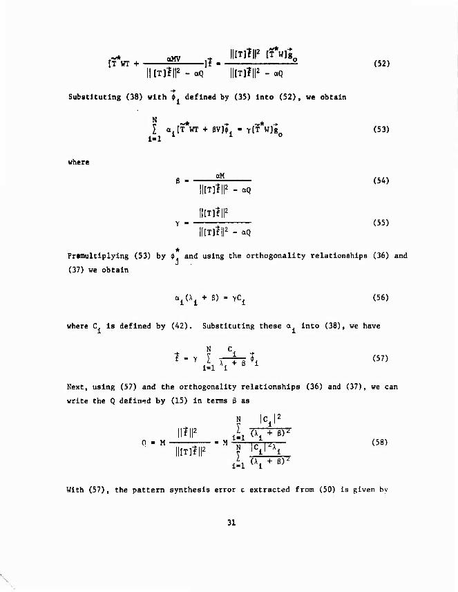
[T VfT + SSi jl . £ (52) 18,
l|[T]1|I2-aQ'" ||[T]I||2 - aq"
Substituting (38) with $ defined by (35) Into (52), we obtain
N * *
where
I a [T WT + ßVl|. - Y[T Wlgn (53) 1-1 0
aM (54) UtTlUP - aQ
l|[T]f||2
l|[T]f ||2 - aQ
(55)
Premultlplylng (53) by $ and using the orthogonality relationships (36) and
(37) we obtain
a1(A1 + B) - YC1 (56)
where C Is defined by (42). Substituting these a Into (38), we have
N C
^ " Y 1=1 V^ ^ ^^
Next, using (57) and the orthogonality relationships (36) and (37), we can
write the q defined by (15) In terms B as
? |Ci|2 , ll?ll2 ^ ÖTTTF
0 - M M L rfjr- (58) ||[T]?||2 ? ^l1 Xl
With (57), the pattern synthesis error e extracted from (50) is given by
31

Ä N \C\\ N |C P S IcJ2
12 (59)
Manipulation with (54), (55), and (58) results In
! |c'12
ill <xi + ß)'
Equation (60) is more easily obtained by setting to zero the partial
derivative of (59) with respect to Y . SubstitutlnR (60) Into (59),
we finally have
Li (*4+ ß))
r ' 1 1
It is desired to find a > 0 such that (48) is satisfied. Since (58)
expresses Q not in terms of a but in terms of ß, a relation between u and
S must be found. Solving (54) for a, replacing Q by expression (58), and
recalling that ||Tf|{ is proportional to Y given by (60), we obtain
0 M /, XTTB I j ' i1 (62)
1-1 Xl
The derivative of (62) given by
j 1 N |C.|2X.
d8 M1i1(X1 + S)^ (63)
indicates that the right hand side of (62) Is a monotone increasing func-
tion of ß except at ß - - X. for 1-1,2,,..N where it Jumps suddenly from
32
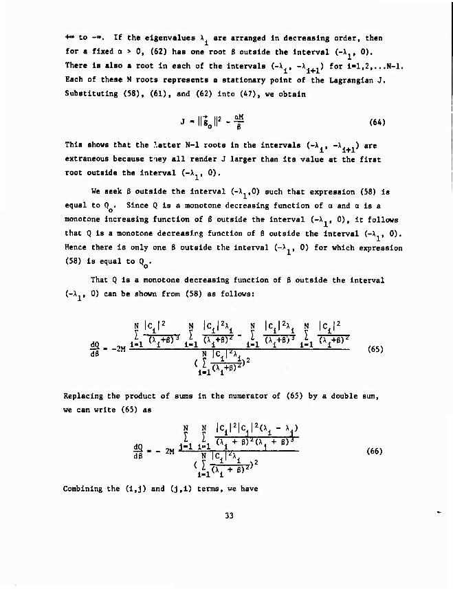
+" to -«. If the eigenvalues X are arranged In decreasing order, then
for a fixed a > 0, (62) has one root 8 outside the interval (-X., 0).
There Is also a root In each of the intervals (-X , -X. ,) for 1-1,2,...N-l.
Each of these N roots represents a stationary point of the Lagranglan J.
Substituting (58), (61), and (62) Into (47), we obtain
J-|li0ll2-y (64)
This shows that the .latter N-l roots in the intervals (-X , -X..,) are
extraneous because t ley all render J larger than its value at the first
root outside the interval (-X , 0).
We seek ß outside the Interval (-X ,0) such that expression (58) is
equal to Q . Since Q is a monotone decreasing function of a and a is a
monotone increasing function of 6 outside the Interval (-X., 0), it follows
that Q is a monotone decreasing function of ß outside the interval (-X , 0).
Hence there is only one ß outside the interval (-*•■» 0) for which expression
(58) is equal to Q .
That Q is a monotone decreasing function of ß outside the interval
(-X., 0) can be shown from (58) as follows:
N IcJ* N IcJ^ N |C1|2X1 N \C±\*
f. .m kMi i-i y^; k v^ ii ^vg! (65)
Replacing the product of sums in the numerator of (65) by a double sum,
we can write (65) as
? v |ci|2lci|2(xi~ V HO i-i ill ^i+ t^K+ &y i--2"11^1!^—j ™
Combining the (l,j) and (J,l) terms, we have
33
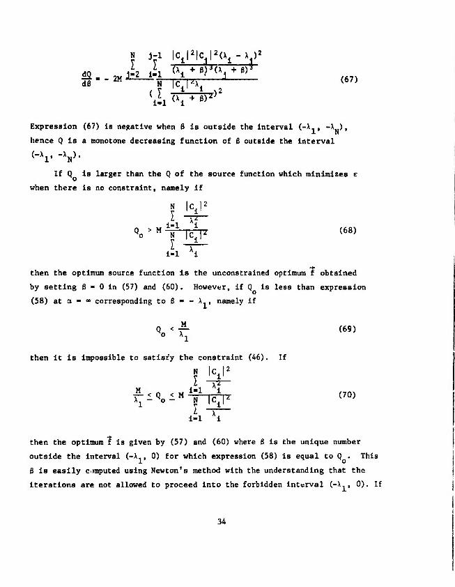
d<? - .tIw ill (xl + 0)'(*1 + a)' dB (67)
Expression (67) Is negative when ß Is outside the Interval (-X, , -X„), 1 N
hence Q Is a monotone decreasing function of ß outside the Interval
("Ai' "V- If Q Is larger than the Q of the source function which minimizes e
when there Is no constraint, namely if
I -T2—
% > M ir-ic7F (68)
i-i Ai
then the optimum source function is the unconstrained optimum f obtained
by setting ß » 0 in (57) and (60). However, If Q Is less than expression
(58) at a - <» corresponding to ß - - X., namely if
Qo < £■ (69) o X1
then it is impossible to satisfy the constraint (46). If
L -T2- flQolMij^V (70)
I - 1-1 Ai
1 - y ^i; L x.
then the optimum f is given by (57) and (60) where ß is the unique number
outside the interval (-X., 0) for which expression (58) is equal to Q . This
ß is easily computed using Newton's method with the understanding that the
iterations are not allowed to proceed into the forbidden interval (-X.., 0). If
34
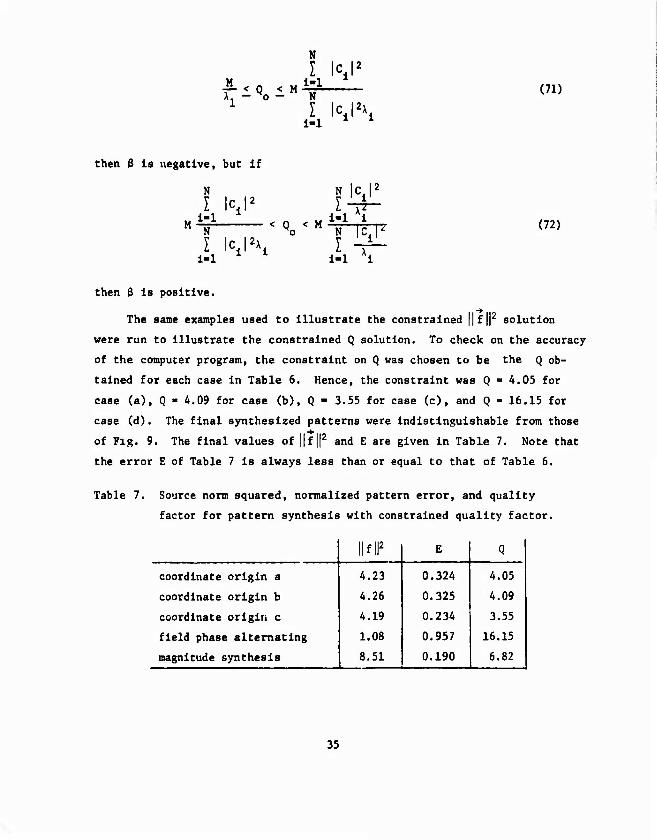
H
(71)
then 8 Is negative, but if
N
.. 1-1 N I \c±\\
1-1
< Q < M o
?lCi 1-1 Al
N
I 1-1
fc^F (72)
then S Is positive.
The sane examples used to illustrate the constrained ||f|p solution
were run to illustrate the constrained Q solution. To check on the accuracy
of the computer program, the constraint on Q was chosen to be the Q ob-
tained for each case in Table 6. Hence, the constraint was Q - 4.05 for
case (a), Q - 4.09 for case (b), Q - 3.55 for case (c), and Q « 16.15 for
case (d) . The final synthesized patterns were indistinguishable from those
of Fig. 9. The final values of ||f ||2 and E are given in Table 7. Note that
the error E of Table 7 Is always less than or equal to that of Table 6.
Table 7. Source norm squared, normalized pattern error, and quality
factor for pattern synthesis with constrained quality factor.
llfll2 E Q |
coordinate origin a 4.23 0.324 4.05
coordinate origin b 4.26 0.325 4.09
coordinate origin c 4.19 0,234 3.55
field phase alternating 1.08 0.957 16.15
magnitude synthesis 8.51 0.190 6.82
35
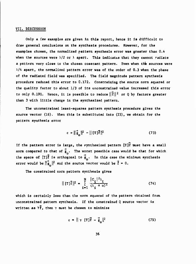
VII. DISCUSSION
Only a few examples are given In this report, hence It la difficult to
draw general conclusions on the synthesis procedures. However, for the
examples chosen, the normalized pattern synthesis error was greater than 0.4
when the sources were Ml or \ apart. This indicates that they cannot radiate
a pattern very close to the chosen cosecant pattern. Even when this sources were
X/A apart, the normalized pattern error was of the order of 0.3 when the phase
of the radiated field was specified. The field magnitude pattern synthesis
procedure reduced this error to 0.172. Constraining the source norm squared or
the quality factor to about 1/3 of its unconstrained value increased this error
to only 0.191. Hence, it is possible to reduce {|f |{2 or Q by factors greater
than 3 with little change in the synthesized pattern.
The unconstrained least-squares pattern synthesis procedure gives the
source vector (16). When this is substituted into (23), we obtain for the
pattern synthesis error
e-||g0ll2-||[T)?||2 (73)
If the pattern error is large, the synthesized pattern [T]f must have a small
norm compared to that of g . The worst possible case would be that for which
the space of [Tjf is orthogonal to g . In this case the minimum synthesis
error would be ||g ||2 and the source vector would be f ■ 0.
o mal to L,
. ,l2 and the source
The constrained norm pattern synthesis gives
N IcJ2^
which is certainly less than the norm squared of the pattern obtained from
unconstrained pattern synthesis. If the constrained Q source vector is
written as Yr, then y must be chosen to minimize
e - II Y IT]I - go||2 (75)
36
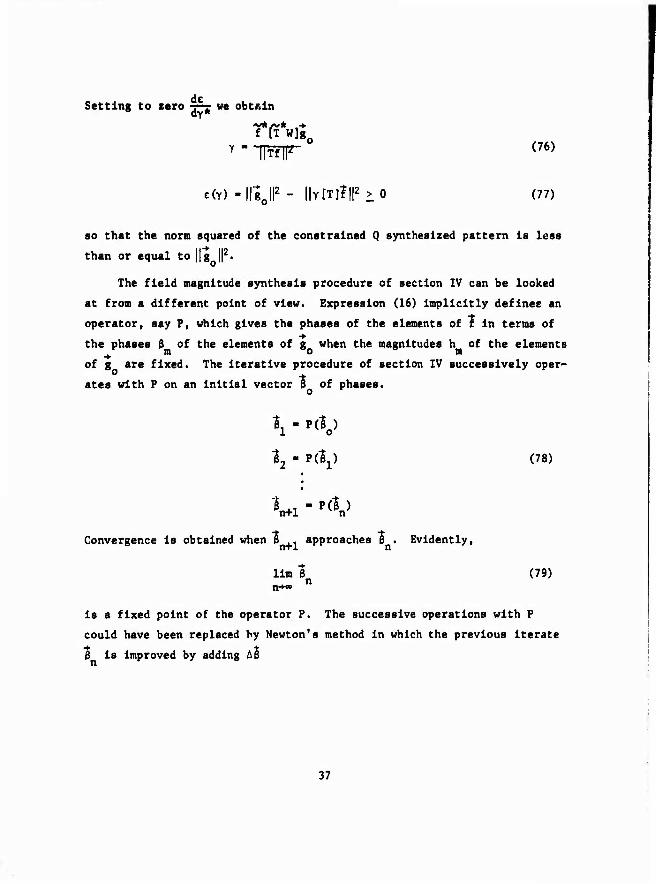
Setting to sero -j—j- we obtain •NM/V* f [T W]
Y - 1W- 0 (76)
E(Y) -llgjl2 - ||Y[T]I||2 > 0 (77)
so that the norm squared of the constrained Q synthesized pattern Is less
than or equal to ||g ||2.
The field magnitude synthesis procedure of section IV can be looked
at from a different point of view. Expression (16) Implicitly defines an
operator, say P, which gives the phases of the elements of f in terms of
the phases 3 of the elements of g when the magnitudes h of the elements m o m of g are fixed. The iterative procedure of section IV successively oper-
ates with F on an initial vector 0 of phases. o r
1 - P(1 ) i o
12 - P^) (78)
\+l " P(V Convergence is obtained when ß .- approaches 8 . Evidently,
lim I (79) n~ n
is a fixed point of the operator P. The successive operations with P
could have been replaced by Newton's method In which the previous Iterate
ß is Improved by adding AS
37
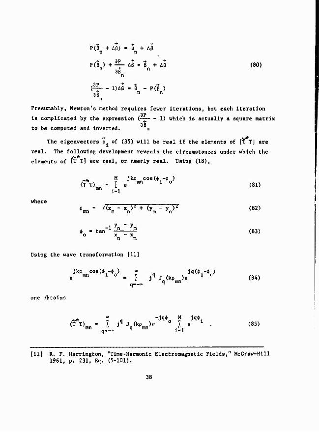
P(l + AS) -I + Aß n n
P(8 ) +i£- Aß - I + Aß (80) n 3ß n
n
(~- - DAß - I - P(ß ) 3ß n n n
Presumably, Newton's method requires fewer iterations, but each Iteration 3P
Is complicated by the expression (— 1) which Is actually a square matrix 3ß to be computed and inverted. n
The eigenvectors $ of (35) will be real If the elements of [TT] are
real. The following development reveals the circumstances under which the
elements of fr T] are real, or nearly real. Using (18),
(T T) - I e ** 1 0 (81) m 1-1
where P, = /(xm - *)' + (y - y )^ (82) mn m n m n
^ - tan 1 -2 E (83) o x - X
n m
Using the wave transformation [11]
ä mn i 0 - E Jq J (kp^)« 1 0 (84) q mn q—-a» ^
one obtains
(TV - I J^JOcP^r 0 I e"1 . (85) mn q mn . ^ n
[11] R. F. Harrington, "Time-Harmonic Electromagnetic Fields," McGraw-Hill 1961, p. 231, Eq. (5-101).
38

Since the $. are equally spaced and because 4. can be absorbed Into $ ,
we are at liberty to take
*1 " (1'1) T (86)
in which case
M Jq*. r.
i-1
M q - an integer multiple of M I e 1 -• (87)
0 otherwise
whence
or
«* r Ma ";,Mq*o (T T) - M [ jMq JM (kp )e 0 (88)
/v* (TT) - M[J (kp ) + 2 I JMqJM (kpnm)cos(Mq4 )] (89) mn o mn , nq mn o
q-1
Hence (T T) is real whenever M is even. If M is odd, then (T T) is mn mn
nearly real whenever M >> kp because from the table on page 407 of [12]
J (x) is very small when n >> x. n
Newton's method was used to find the root a of (45) and the root 6 of
(48) where Q is given by (58). However, if the starting value is far from
the root, the first few Iterates of Newton's method are probably not very
well directed because the change In the variable a or ß from one iteration
to the next is not a good indicator. In the beginning, an Interval halving
procedure would probably give as much improvement per iteration and take a
lot less time per iteration because the derivative need not be calculated.
However, the interval halving procedure requires a negative and a positive
value of the function in order to start. Also, it would be difficult to
decide when to change from interval halving to Newton's method. Newton's
[12] M. Abramowltz and I. A. Stegun, "Handbook of Mathematical Functions with Formulas, Graphs, and Mafbematlcal Tables," National Bureau of Standards, 1964, pp. 355-433.
39

method may be modified by replacing Che derivative by a finite difference
approximation, but then It Is feared that the time saved per Iteration may
be offset by slower convergence.
The computer programs, with operating Instructions and sample input-
output data, for all the examples of this report will be given in Scientific
Report No. 3 of this contract. It is hoped that further examples wlyll be run
in the future to better assess the capabilities of these synthesis programs.
40

APPENDIX
ALTERNATIVE METHOD FOR FIELD MAGNITUDE PATTERN SYNTHESIS
An alternativ« method for field magnitude synthesis Is as follows.
Expression (21) can be rewritten as
e(f,S) - - 2 Real(e w^ £ fj ) n"l
w h + w. N
'", n In n"l
2 M + y w mil * mfll
I f T - h e m
''. n mn m n-1
(A-l)
The minimum of expression (A-l) with respect to ß. occurs when 6. Is the
tigle of l fnT n*l n In
Thus It Is possible to minimize (21) with respect
to 0. for 1 ■ 1,2,...M. The proposed alternative method for field magnitude
synthesis consists of minimizing (21) successively with respect to
B,, B.I...BU> 6,t Bol.<.Bul etc. Hence, one angle Is changed at a time In i z n L i n
this method, compared to all angles being changed at once In the method used
In the text. It Is not known which method converges faster, since tests were
not made.
41

REFERENCES
[1] For example, see R. E. Collln and F. J. Zucker, "Antenna Theory," Part 1, McGraw-Hill Book Co., New York, 1969, Chap. 7.
[2] G. A. Deschamps and H. S. Cabayan, "Antenna Synthesis and Solution of Inverse Problems by Regularlzatlon Methods," IEEE Trans., vol. AP-20, No. 3, May 1972, pp. 268-274.
[3] A. N. Tlhonov, "Solution of Incorrectly Formulated Problems and the Regularlzatlon Method," Soviet Mathematics, vol. 4, July-December 1963, pp. 1035-1038.
[4] V. I. Popovkln and V. I. Yelumeyev, "Optimization and Systematlzatlon of Solutions to Antenna Synthesis Problems," Radio Engineering and Electronic Physics, vol. 13, No. 5, 1968, pp. 682-686.
[5] V. I. Popovkln, G. I. Shcherbakov, V. I. Yelumeyev, "Optimum Solutions of Problems in Antenna Synthesis Theory," Radio Engineering and Electronic Physics, vol. 14, No. 7, 1969, pp. 1025-1030.
[6] L. D. Bakhrakh and V. I. Troytskly, "Mixed Problems of Antenna Synthesis," Radio Engineering ana Electronic Physics, vol. 12, No. 3, March 1967, pp. 404-414. "w"~
[7] Y. I. Choni, "Synthesis of an Antenna According to a Given Amplitude Radiation Pattern," Radio Engineering and Electronic Physics, vol. 16, No. 5, May 1971, pp. 770-778. ~ ™-™.— ,-,-._
[8] R. F. Harrington and J. R. Mautz, "Synthesis of Loaded N-port Scatterers," AFCRL-72-0665, Scientific Report No. 17 on Contract No. F19628-68-C-0180 between Syracuse University and Air Force Cambridge Research Laboratories, October 1972.
[9] R. F. Harrington, "Field Computation by Moment Methods," Macmlllan Co., New York, 1968.
[10] Y. T. Lo, S. W. Lee, and Q. H. Lee, "Optimization of Directivity and Signal-to-Nolse Ratio of an Arbitrary Antenna Array," Proc. IEEE, vol. 54, August 1966, pp. 1033-1045.
[11] R. F. Harrington, "Tlme-Harmonlc Electromagnetic Fields," McGraw-Hill, 1961, p. 231, Eq. (5-101).
[12] M. Abramowitz and I. A. Stegun, "Handbook of Mathematical Functions with Formulas, Graphs, and Mathematical Tables," National Bureau of Standards, 1964, pp. 355-433.
42
Top Related