


Languages
Pages
Legal


DISCUSSION PAPER SERIES
ABCD
www.cepr.org
Available online at: www.cepr.org/pubs/dps/DP9533.asp www.ssrn.com/xxx/xxx/xxx
No. 9533
CORPORATE SOCIAL RESPONSIBILITY AND FIRM RISK:
THEORY AND EMPIRICAL EVIDENCE
Rui Albuquerque, Artyom Durnev and Yrjö Koskinen
FINANCIAL ECONOMICS and INDUSTRIAL ORGANIZATION

ISSN 0265-8003
CORPORATE SOCIAL RESPONSIBILITY AND FIRM RISK: THEORY AND EMPIRICAL EVIDENCE
Rui Albuquerque, Boston University Católica-Lisboa School of Business and Economics, ECGI and CEPR
Artyom Durnev, University of Iowa Yrjö Koskinen, Boston University and CEPR
Discussion Paper No. 9533 July 2013
Centre for Economic Policy Research 77 Bastwick Street, London EC1V 3PZ, UK
Tel: (44 20) 7183 8801, Fax: (44 20) 7183 8820 Email: [email protected], Website: www.cepr.org
This Discussion Paper is issued under the auspices of the Centre’s research programme in FINANCIAL ECONOMICS and INDUSTRIAL ORGANIZATION. Any opinions expressed here are those of the author(s) and not those of the Centre for Economic Policy Research. Research disseminated by CEPR may include views on policy, but the Centre itself takes no institutional policy positions.
The Centre for Economic Policy Research was established in 1983 as an educational charity, to promote independent analysis and public discussion of open economies and the relations among them. It is pluralist and non-partisan, bringing economic research to bear on the analysis of medium- and long-run policy questions.
These Discussion Papers often represent preliminary or incomplete work, circulated to encourage discussion and comment. Citation and use of such a paper should take account of its provisional character.
Copyright: Rui Albuquerque, Artyom Durnev and Yrjö Koskinen

CEPR Discussion Paper No. 9533
July 2013
ABSTRACT
Corporate Social Responsibility and Firm Risk: Theory and Empirical Evidence*
This paper presents an industry equilibrium model where firms can choose to engage in corporate social responsibility (CSR) activities. We model CSR activities as an investment in customer loyalty and show that CSR decreases systematic risk and increases firm value. These effects are stronger for firms producing differentiated goods and when consumers' expenditure share on CSR goods is small. We find supporting evidence for our predictions. In our empirical tests, we address a potential endogeneity problem by instrumenting CSR using data on the political affiliation of the firm's home state, and data on environmental and engineering disasters and product recalls.
JEL Classification: D43, G12, G32, L13 and M14 Keywords: corporate social responsibility, corporate valuation, customer loyalty, industry equilibrium and systematic risk
Rui Albuquerque School of Management Boston University 595 Commonwealth Avenue Boston, MA 02215 USA Email: [email protected] For further Discussion Papers by this author see: www.cepr.org/pubs/new-dps/dplist.asp?authorid=147792
Artyom Durnev Tippie College of Business University of Iowa 108 John Pappajohn Building Iowa City, IA 52242 USA Email: [email protected] For further Discussion Papers by this author see: www.cepr.org/pubs/new-dps/dplist.asp?authorid=156806
Yrjö Koskinen School of Management Boston University 595 Commonwealth Avenue Boston, MA 02215 USA Email: [email protected] For further Discussion Papers by this author see: www.cepr.org/pubs/new-dps/dplist.asp?authorid=146686
*We thank C. B. Bhattacharya, Ruslan Goyenko, Jonathan Karpoff, Anders Loflund, Robert Marquez, Laura Starks, Chen Xue, Chendi Zhang and seminar participants at the BSI Gamma Foundation Conference in Venice, the CalPERS and UC Davis Sustainability & Finance Symposium, the 2012 FIRS conference, 2nd Helsinki Finance Summit, Geneva Summit on Sustainable Finance, Imperial College Business School, Boston University, University of Iowa and Warwick Business School for their comments. We also thank the BSI Gamma Foundation for a research grant and the Geneva Summit on Sustainable Finance for the Best Paper Prize. Albuquerque gratefully acknowledges the financial support from a grant from the Fundação para a Ciência e Tecnologia. The research leading to these results has received funding from the European Union Seventh Framework Programme (FP7/2007-2013) under grant agreement PCOFUND-GA-2009-246542 and from the Foundation for Science and Technology of Portugal.
Submitted 24 June 2013

1 Introduction
Corporate social responsibility (CSR) represents a growing strategic concern for corpora-
tions around the world, many of which are adopting CSR as a core management or board-
level function. The Global Reporting Initiative (GRI) founded in the late 1990’s, taken on
by the United Nations Environment Program, has provided corporations with a reporting
framework on their economic, environmental, and social sustainability. The success of this
initiative is visible in the widespread integration of its reporting framework within regular
company annual reports.1 Arguably, CSR’s increased popularity inside boardrooms has
outpaced the research needed to justify it.2 No longer necessarily viewed outside the profit
maximizing framework, many questions still remain on how CSR policies a§ect the risks
firms are facing and the stock market implications of those policies (Bénabou and Tirole,
2010, and Starks, 2009).3 In this paper, we aim to address these issues by proposing a
theory of how CSR a§ects firms’ systematic risk and market value. We follow then by
providing empirical evidence supporting our proposed mechanism.
We develop an industry equilibrium model where firms make production and CSR invest-
ment decisions and embed this model within a standard asset pricing framework. Following
an extensive marketing literature (see e.g. Luo and Bhattacharya, 2006, 2009), we model an
investment in CSR as a mechanism to acquire customer loyalty. Greater customer loyalty
takes the form of a less price elastic demand, which the firm uses to smooth out the e§ect
of aggregate economic fluctuations. With this assumption, the model captures the widely
held view in the marketing literature that a firm with a more loyal demand has profits that
1 Intel Corporation provides a good example of the GRI reporting framework. CSR forms a part of Intel’sintegrated value approach with quantitative metrics for its CSR policies. Intel’s Corporate ResponsibilityReport for 2012 can be found at http://csrreportbuilder.intel.com/PDFFiles/CSR_2012._Full-Report.pdf
2 In 2008, the Economist wrote to attest to the popularity of CSR that “The CSR industry, as we haveseen, is in rude health. Company after company has been shaken into adopting a CSR policy: it is almostunthinkable today for a big global corporation to be without one.”
3For example, Bénabou and Tirole (2010, p. 9) argue that: “Corporate social responsibility (CSR) issomewhat of a ‘catch-all’ phrase for an array of di§erent concepts. An analysis of CSR must therefore clarifyits exact meaning, and in particular the presumed impact of CSR on the cost of capital.”
1

are relatively less sensitive to aggregate economic conditions than a firm with a less loyal
demand. From the perspective of a risk averse investor, a firm facing a more loyal demand
exhibits lower systematic risk and is valued more highly.
The benefit from CSR adoption as a risk management tool is a partial equilibrium e§ect
that contrasts with an industry-equilibrium feedback e§ect. Greater customer loyalty gives
CSR adopters higher operating profits per unit of revenue. This in turn leads more firms to
adopt CSR policies and firms with higher adoption costs implement CSR policies as well.
These higher adoption costs increase operating leverage and lead to increasing systematic
risk for the marginal firm.
We show that the relative strength of these two e§ects, and thus the relative riskiness
of CSR firms, depends on the representative consumer’s expenditure share on CSR goods.
A su¢ciently small expenditure share on CSR limits the proportion of CSR firms and
implies that the marginal CSR firm has a lower systematic risk and a higher valuation
than non-CSR firms. Therefore, the two main model predictions are that high-CSR firms
have lower systematic risk and higher firm values. Moreover, since lower systematic risk is
associated with lower co-movement of net profits with aggregate economic conditions, the
model predicts that the ratio of net profits of CSR firms relative to that of non-CSR firms
decreases in economic expansions.
The industry equilibrium of the model also allows us to study the e§ects of CSR adoption
across industries. These additional predictions are important indirect tests of the model’s
hypothesis that CSR helps build customer loyalty. The model predicts that industries with
greater product di§erentiation have a stronger CSR-risk relation, and that industries with
a larger consumer’s expenditure share on CSR goods have a weaker CSR-risk relation.
This second prediction is somewhat surprising and is explained by the fact that increased
spending in CSR results in the marginal CSR firm having higher adoption costs, higher
operating leverage and systematic risk. The opposite occurs for non-CSR firms at the same
2

time: fewer firms produce with non-CSR technologies and with less competition these firms
obtain higher profit margins, lowering their operating leverage and systematic risk.
We test the model predictions using a comprehensive dataset on firm-level CSR from
MSCI’s Environmental, Social and Governance (ESG) database. The sample consists of
a panel of U.S. firms spanning the years from 2003 to 2011 with a total 23,803 firm-year
observations. From ESG we obtain a firm-level CSR score that aggregates six di§erent
ratings attributes: community, diversity, employee relations, environment, product, and
human rights. ESG also includes a governance attribute. To separate our analysis from
studies that focus on governance related topics, our main results exclude the governance
attribute from the firm’s aggregate CSR score, but we also show the result of including the
governance attribute with all other CSR attributes. We estimate firm systematic risk using
a three factor model of returns and, following our model, take firm beta to be the coe¢cient
on the market return. We run panel regressions with firm and year fixed e§ects, and with
and without control variables that are known to a§ect systematic risk.
We first document that the level of systematic risk is statistically and economically
significantly lower for firms with a higher CSR score. One standard deviation increase in
firm CSR score reduces firm beta on average by 0.036, which represents a 4% decline in
systematic risk relative to the sample mean 0.914. This e§ect does not appear to be caused
by any single CSR attribute though the attributes diversity and environment have the
largest economic impact whereas the attributes product and governance have a statistically
insignificant impact. We then estimate the e§ect of CSR on systematic risk year by year and
show that CSR exhibits a significantly negative impact on firm beta every year except for
the years 2003 and 2009, when the impact of CSR is negative but insignificantly di§erent
from zero. Consistent with the risk mechanism in our model and the customer loyalty
assumption, we also provide evidence that the ratio of CSR firms’ profits to non-CSR firms’
profits is negatively related to GDP growth.
3

Next, we find evidence supportive of the prediction that the e§ect of CSR on firm beta is
stronger in industries with greater product di§erentiation. We use two measures of product
di§erentiation. One measure is a dummy variable that takes the value of one if the firm
operates in a di§erentiated goods industry as defined by Giannetti et al. (2011). Another
measure is the continuous, firm-level product similarity variable developed in Hoberg and
Phillips (2010). We find that the economic magnitude of the e§ect of CSR on firm beta
is 34% higher in di§erentiated goods industries and 46% higher in firms with zero product
similarity as compared to the sample mean of product similarity. We also find evidence
supportive of the prediction that industries with a larger expenditure share on CSR goods
have a weaker CSR-risk relation. In our model, increased consumer spending in CSR
translates into a relatively larger number of firms that adopt CSR policies in an industry
and increases the relative valuation of these firms. We therefore test whether the stock
market capitalization of the higher-rated CSR firms is associated with a smaller di§erence
in firm betas across CSR and non-CSR firms within an industry. We find that in industries
where the top CSR firms have a higher relative market capitalization, the impact of CSR
on beta is reduced, consistent with the model.
We find that higher CSR score has a positive impact on Tobin’s Q. A one standard
deviation increase in CSR score increases firm value by 0.136, equivalent to 7.07% of the
sample mean of Tobin’s Q of 1.927. Consistent with the model, this e§ect is larger for firms
that produce di§erentiated goods. In addition, the impact of CSR on firm value is lower
when top CSR firms have higher market capitalization.
Endogeneity is a major concern in the existing CSR literature, because it may be that
a firm’s financial performance is a determinant in its CSR decisions. Alternatively, more in
the spirit of our story, firms that build customer loyalty through branding, and thus have
lower systematic risk, might also do more CSR. In order to address these concerns, we run
our tests with a comprehensive set of control variables. In addition, we address endogeneity
4

concerns by employing two novel sets of instruments for CSR. The first instrument is based
on political a¢liation of the state where the company is headquartered. As shown by Di
Giuli and Kostovetsky (2012), firms headquartered in Democratic-leaning states are more
likely to spend more resources on CSR. However, the political a¢liation of a state should
be unrelated to systematic risk and firm value.
The second instrument is based on a sample of product recalls, and environmental and
engineering disasters. We argue that these are good instruments because MSCI’s construc-
tion of the CSR score relies on some of the same information. In addition, the perception of
CSR is likely to decrease following a disaster and, while the likelihood of disasters may lead
to increases in idiosyncratic risk and lower firm value, for example due to the risk of law
suits, it is unlikely that firm beta is related to these exogenous incidents. In our tests, we
cannot reject that both of these sets of instruments are exogenous. We find that when we
use the political a¢liation of the firm’s state of headquarter as the instrument, the instru-
mented CSR is negatively related to systematic risk and positively related to firm value,
as predicted. When we use product recalls and environmental and engineering disasters as
the instrument, the instrumented CSR is negatively related to beta. The results from the
instrumental variables approach yield higher economic significance e§ects than the results
using ordinary least squares and provide strong support that CSR leads to lower systematic
risk and higher valuations, not the other way around. We deem these results to be one of
our main contributions.
We organize the rest of the paper as follows. Section 2 reviews the existing literature.
Section 3 presents the model and derives its equilibrium. Section 4 analyzes the equilibrium
properties regarding risk and firm value. Section 5 presents the data used in our empirical
tests and Section 6 presents the results. Section 7 concludes the paper. Proofs are relegated
to the appendix as is an extension of the model to an infinite horizon setting.
5

2 Related Literature
A growing literature asserts that firms engage in profit maximizing CSR (e.g., Baron, 2001,
and McWilliams and Siegel, 2001). According to the profit maximizing view, firms un-
dertake CSR activities because they expect a net benefit from them.4 Our paper fits into
a line of research whereby profit maximizing CSR is a product di§erentiation strategy to
gain competitive advantage over one’s rivals (see Navarro, 1988, Webb, 1996, Bagnoli and
Watts, 2003, and Siegel and Vitalino, 2007).5 There is empirical evidence supporting the
conjecture that CSR policies a§ect consumer behavior. Creyer (1997) shows that corporate
ethical behavior a§ects positively consumers’ purchase intentions. Auger et al. (2003) and
Pelsmacker et al. (2005) document consumer willingness to pay for ethical product features.
Ailawadi et al. (2011) provide evidence that in a retail setting, consumers are willing to
pay for product and employee related intrinsic CSR activities, but not for extrinsic CSR
activities such as environmental and social programs. Elfenbein and McManus (2010) and
Elfenbein et al. (2012) show using data from eBay auctions that customers pay more for
products sold through charity auctions, than those in non-charity auctions, and have fewer
complaints among charity-intensive sellers.
CSR has received scant attention in theoretical finance literature. A notable exception
is Heinkel et al. (2001), who assume that some investors choose not to invest in non-CSR
stocks. This market segmentation leads to higher expected returns for non-CSR stocks,
which must be held by only a fraction of the investors (as in Errunza and Losq, 1985, and
Merton, 1987). In addition, Barnea et al. (2009) derive a model where ethical investors
increase the value for CSR stocks and firms respond by choosing endogenously their level
4According to Bénabou and Tirole (2010), the other motivations for CSR policies are delegated philan-thropy and agency costs. In delegated philanthropy stakeholders delegate social activities they would like todo themselves to corporations. With agency costs, managers engage in CSR activities because they receiveprivate benefits from them.
5 In an international survey of CEOs, Hopkins and Cowe (2004) report that 79% of respondents say thatCSR is necessary to maintain a competitive advantage.
6

of CSR spending. Gollier and Pouget (2012) build a model where socially responsible
investors can take over non-CSR companies and create value by turning those into CSR
companies. All these papers assume that there is a class of investors who prefer to invest in
CSR stocks. However, as pointed out by Starks (2009), investors seem to care more about
corporate governance than CSR. In contrast, our paper does not assume that investors care
about CSR and instead focuses on the role of consumers and their actions, based on their
perceptions of corporate responsible policies.
There is some recent empirical literature that documents a link between CSR, system-
atic risk and cost of equity capital. Sharfman and Fernando (2008) show that firm-level
environmental performance is negatively associated with systematic risk resulting in lower
cost of equity capital. Their sample size is small (270 firms) and is only cross-sectional.
Using a panel data set of S&P 500 firms, Oikonomou et al. (2012) confirm that CSR is neg-
atively related to systematic risk, in particular that social irresponsibility (CSR concerns)
is associated with higher systematic risk. El Ghoul et al. (2011), calculating an ex-ante
measure for cost of equity that utilizes analysts estimates, find that firms with higher CSR
scores exhibit lower cost of capital.
Our paper is also related to the empirical literature on the association of CSR and firm
value or shareholder wealth. Margolis et al. (2009) review the older empirical evidence
and show that there is on average a small positive e§ect. Galema et al. (2008) provide
evidence that CSR stocks have lower book-to-market ratios, i.e. that CSR stocks exhibit
higher valuations. Gillan et al. (2010) show that environmental and governance scores are
positively related to firm value, measured by Tobin’s Q. CSR firms have also higher return
on assets, due to lower operating expenses. Servaes and Tamayo (2012) provide evidence
of positive association with CSR and firm value, but only for firms with high advertising
expenditures. Using an event-studies approach, Fisher-Vanden and Thorburn (2011) find
that when firms announce their membership in the Environmental Protection Agency’s
7
Climate Leaders, a program intended to reduce greenhouse gas emissions, the announcement
is met with negative abnormal returns. Like Fisher-Vanden and Thorburn, Krüger (2012)
shows, in a larger sample of CSR events, that unconditionally both negative and positive
CSR news lead to a stock price decline. However, in Krüger’s study, the wealth e§ect of
positive CSR news depends on the motivation of the management: there is a negative e§ect
on stock prices if management is likely to receive private benefits from CSR adoption, but a
positive e§ect if CSR policies are adopted to improve relations with stakeholders.6 Dimson
et al. (2012) analyze CSR activism conducted by a large institutional investor and show
that, consistent with Krüger’s study, positive engagements that lead to changes in firms’
CSR policies are followed by positive abnormal returns.
Some papers study the stock market performance of CSR stocks. The evidence is mixed.
Brammer et al. (2006) and Hong and Kacperczyk (2009) find that least socially desirable
stocks have higher expected returns after controlling for risk. Becchetti and Ciciretti (2009)
provide evidence that for CSR stocks there is no di§erence in buy-and-hold risk adjusted
returns relative to the control sample. In contrast, Derwall et al. (2005) show that the most
ecologically e¢cient firms experience higher expected returns that cannot be accounted for
by risk factors and Kempf and Ostho§ (2007) show that a strategy whereby they invest in
the most socially responsible stocks and short sell the least socially responsible ones leads
to positive abnormal returns.7
We contribute significantly and provide novel insights to the existing literature on CSR.
First, our paper builds a model based on customer loyalty and employs a standard con-
sumption based asset pricing model embedded in an industry equilibrium model. Thus,
6Cheng et al. (2013) provide evidence that increase in after-tax e§ective managerial ownership leads todecrease in CSR activities. This is a marginal e§ect and does not show that on average CSR activities aredue to agency costs.
7There is also a literature examining the performance of socially reponsible mutual funds. Geczy et al.(2003) show the cost of restricting investments to socially responsible funds is small, but that this cost issignificant when size, value and momentum factors are controlled for. Renneboog et al. (2008) show thatsocially responsible mutual funds underperform their benchmarks, though by not more than conventionalmutual funds, except for a small number of countries.
8
we provide a novel theoretical justification for the existing empirical findings. Second, we
derive new testable implications (namely, that the e§ect of CSR on systematic risk is larger
for firms producing di§erentiated goods, that the e§ect is weaker when consumers’ expen-
diture share on CSR goods is higher, and that the ratio of CSR profits to non-CSR profits
is countercyclical) and find empirical support for these implications. Third, we utilize a
larger data set than previous studies and control for other possible e§ects carefully. Fourth,
we consider the possibility of reverse causality and construct instruments for CSR that can
help us mitigate the endogeneity concern.
Lastly, our paper is related to the work on brand assets and firm risk, since both branding
and CSR a§ect consumer behavior. Rego et al. (2009) find a negative relation between a
firm’s brand equity, measured by consumers brand beliefs that a§ect purchase behavior,
and firm risk. Brand equity has a negative impact especially on idiosyncratic risk, but
also protects shareholders from systematic risk. Belo et al. (2011) find that firms with
higher investments in brand capital, measured by advertising expenditures, exhibit lower
stock returns compared to firms with lower investments in brand capital. The reason is
that firms that invest more in brand capital are also the most productive firms with low
systematic risk. In our empirical tests, we show that the e§ect of CSR on systematic risk
is robust to controlling for advertising expenditures. Thus, we can conclude that CSR has
an independent role in a§ecting firm risk.
3 The Model
3.1 The model setup
Consider an economy where production, asset allocation, and consumption decisions are
made over two dates, 1 and 2. There is a representative investor and a continuum of firms
with unit mass. For generality, we present an extension to infinite horizon in the Appendix.
9

Household sector: The representative investor has preferences defined over lifetime con-
sumption
U (C1, C2) =C11
1 + E
"C12
1
#. (1)
The relative risk aversion coe¢cient is > 0 and the parameter < 1 is the rate of time
preference. The expectations operator is denoted by E [.].
There are two types of goods in the economy. Low elasticity of substitution goods,
which we associate with goods produced by socially responsible firms (CSR goods), and high
elasticity of substitution goods, which we associate with other firms (non-CSR goods).8 We
label these using the subscripts G and P , respectively, for green and polluting. A convenient
analytical way to model di§erences in the elasticity of substitution across goods is to use
the Dixit-Stiglitz aggregator,
C2 =
Z µ
0cGi di
G
Z 1
µcPi di
1P
.
Accordingly, 0 < j < 1 is the elasticity of substitution within cj = cG, cP goods. A
lower elasticity of substitution implies lower price elasticity of demand and a more “loyal”
demand. We therefore are interested in the case G < P . This mathematical formulation
of demand loyalty captures two important dimensions of consumer behavior: consumers
that actively seek out firms they see as being good at CSR and consumers that respond
negatively to businesses that fall below expected ethical standards (e.g. Creyer, 1997). The
parameter is the share of expenditure allocated to CSR goods in the industry and is
exogenous. In the context of our representative agent model, captures the size of the
market for CSR goods. The variable µ measures the fraction of CSR firms in the economy
and will be determined in equilibrium.
Investor optimization is subject to two single-period budget constraints. At date 1, the
8The marketing literature provides evidence supportive of a positive association between customer loyaltyand CSR (Creyer 1997, Auger et al., 2003, Pelsmacker et al., 2005, among others). See also Luo andBhattacharya (2006, 2009).
10

investor is endowed with stocks and with cash W1 > 0 expressed in units of the aggregate
good, which can be used for consumption and investment. The investor decides on the date
1 consumption, C1, stock holdings, Di, and the total amount of lending to firms, B, subject
to the date 1 budget constraint,
Z 1
0Qidi+W1 C1 +
Z 1
0QiDidi+B, (2)
and given the stock prices Qi and the interest rate r. The presence ofR 10 Qidi on the left
hand side of the budget constraint (2) indicates, as is usual in models with a representative
investor, that the representative investor is both the seller and the buyer of stocks.
The investor decides on the date 2 consumption of the various goods ci, subject to the
date 2 budget constraint:
W2 ZDi (i Bi (1 + r)) di+ wL+B (1 + r)
Zpicidi. (3)
In the budget constraint, i is the operating profit generated by firm i and Bi (1 + r) is the
debt repayment by firm i so that i Bi (1 + r) is the net profit, and in this two-period
model it is also a liquidating dividend. W2 denotes the consumer’s wealth at the beginning
of date 2, w is the wage rate, L is the amount of labor inelastically supplied and pi is the
price of good i. The investor behaves competitively and takes prices as given.
Production sector: At date 1, firms choose which production technology to invest in.
The decision is based on expected operating profitability and fixed adoption costs. Each
firm is endowed with a technology-adoption cost. Firm i faces a cost of fGi if it chooses to
invest in the CSR technology or a cost fP > 0 if it chooses the non-CSR technology. The
distribution of costs fGi across firms is a uniform that takes values between 0 and 1. Firm
i finances fi by raising debt Bi and therefore has zero cash flow at date 1.
Note that a higher cost fGi does not translate into a higher benefit for CSR firms.
Instead, all CSR firms have access to the same elasticity of substitution, G, independently
11
of their fixed cost of investment. This assumption captures the idea that CSR adoption is
not equally costly to all firms.9 Technically, it introduces decreasing returns to CSR at the
industry level, which helps in the derivation of equilibria with interior values for µ.
At date 2, firm i chooses how much to produce of xi in order to maximize operating
profits. Firms act as monopolistic competitors solving:
i = maxxi{pi (xi)xi wli} , (4)
subject to the equilibrium inverse demand function pi (xi) as well as the constant returns
to scale production technology,
li = Aiixi. (5)
Production of one unit of output requires Aii units of labor input. i measures the sen-
sitivity of firm i’s labor to the productivity shock A and i measures the resource intensity
of each technology. We make no assumption regarding the relative magnitudes of G and
P and of G and P , though some views of CSR might be associated with the assumptions
that CSR firms foster employee loyalty, i.e., G < P , or are more resource intensive, i.e.,
G > P .
The economy is subject to an aggregate productivity shock, A, realized at date 2 before
production takes place. The productivity shock changes the number of labor units needed
to produce consumption goods. High aggregate productivity is characterized by low values
of A. The productivity shock A is assumed to have bounded support in the positive real
numbers.9There are several reasons why fixed costs of adopting CSR technologies may di§er between firms. For
example, costs of converting to organic farming may depend on past chemical use; younger firms, using newerand cleaner technologies, may have lower costs of adopting additional green measures and targets relativeto older firms that may be more likely to use older and more polluting legacy technologies; governmentsubsidies may help promote the use of alternative energies and firms with stronger R&D teams may bebetter positioned to take advantage of these subsidies; and firms with higher quality corporate governancemay have better organizational capabilities of adopting green technologies (Amore and Bennedsen, 2013).
12

Market clearing: In equilibrium, at date 1, asset markets clear, Di = 1, for all i, and
B =RBidi. At date 2, goods markets clear, xi = ci, for all i, and the labor market clears,
Rlidi = L.
3.2 Equilibrium
We start by solving the equilibrium at date 2.
Date-2 equilibrium: Let µ 2 (0, 1) denote the fraction of CSR firms. The outcome of
the date-2 equilibrium is given as a function of the value of µ which is solved for in the
date-1 equilibrium.
Consider the consumer’s problem. Let denote the Lagrange multiplier associated with
the date-2 budget constraint (3). The first order condition for each CSR good cl is
C2
Z µ
0cGi di
G1Z 1
µcPi di
1P
cG1l = pl. (6)
There is a similar condition for each non-CSR good. Multiplying both sides of each first
order condition by the respective cj and integrating over the relevant range gives
C12 =
Z µ
0picidi, (7)
and
(1 )C12 =
Z 1
µpjcjdj. (8)
By taking the ratio of these two conditions, it is straightforward to see that the parameter
gives the expenditure share of CSR goods. The appendix provides the remaining steps
that allow us to solve for the demand functions,
cl = p
1G1l
R µ0 p
GG1i di
W2, (9)
ck = (1 )p
1P1k
R 1µ p
PP1i di
W2, (10)
13
for CSR and non-CSR goods, respectively. Firm j’s demand elasticity equals 11j . Thus,
a lower elasticity of substitution (lower j) is associated with a demand that is less sensitive
to price fluctuations and is therefore more loyal.
It remains to find the value of as a function of goods prices and date 2 wealth.
Adding up (7) and (8) gives C12 = W2. Finally, replacing the demand functions into the
consumption aggregator gives the value of .
We now turn to the firms’ problem. Each firm acts as a monopolistic competitor and
chooses xi according to equation (4). The first order conditions are:
Gpl = wAll,
P pk = wAkk.
The second order condition for each firm is met because 0 < j < 1. Using these first order
conditions, we get the optimal value of operating profits,
j = (1 j) pjxj . (11)
Goods with lower elasticity of substitution j , i.e. goods with more loyal demand, allow
producers to extract higher profits per unit of revenue, all else equal.
To solve for the equilibrium, Walras’ law requires that a price normalization be imposed.
We impose that the price of the aggregate consumption good is time invariant, so its price
at date 2 equals the price at date 1, which is 1. This normalization imposes the following
implicit constraint on prices pl:
1 = minci2{ci:C2=1}
Z 1
0picidi.
The price normalization implies that W2 =Rplcldl = C2, from which we obtain the usual
condition for the marginal utility of date-2 wealth with constant relative risk aversion pref-
erences, = C2 . The next proposition describes the date-2 equilibrium as a function of
µ. The proof is relegated to the Appendix.
14

Proposition 1 For any interior value of µ and any aggregate shock A, a symmetric date-2
equilibrium exists and is unique with goods prices,
pG = pA(1)(GP )PG
GP,
pP = pA(GP ),
consumption,
cG =PP
GGx
µAG ,
cP = x1 1 µ
AP ,
wage rate,
w = pAPP,
operating profits,
G = px (1 G)
µA,
P = px (1 P )1 1 µ
A,
and marginal utility of wealth,
= [px] A,
where p, x > 0 are functions of exogenous parameters given in the Appendix, and =
(1 ) P + G.
In equilibrium, a higher productivity shock (lower A) increases the demand for labor
and thus also increases the wage rate. The sensitivity of the wage rate to the productivity
shock is given by the weighted average of the sensitivities, , where the weights are the
expenditure shares. Prices of goods increase or decrease in response to a productivity shock
depending on which types of goods are more sensitive to the productivity shock, as given
by G P . When G P < 0, the production of non-CSR goods increases in expansions
15

as unit labor costs decrease more for those firms, leading to an increase in the relative price
of CSR goods. The opposite occurs if G P > 0. While the relative price of CSR goods
depends on the sign of G P , operating profits for both firm types, i, and the marginal
utility of date-2 wealth, , depend only upon the weighted average of the sensitivities, .
Date-1 equilibrium: To solve for the date-1 equilibrium, we need to determine the rate
used by the representative investor to discount future profits. Imposing the equilibrium
conditions, the date-1 budget constraint gives C1 = W1 B, so that the intertemporal
marginal rate of substitution, or stochastic discount factor, becomes:
m
C2C1
= m [px] A, (12)
where m = (W1 B) . States of the world with low productivity (high A), and therefore
low aggregate consumption, have higher marginal utility of consumption and higher discount
factor.
The date-1 equilibrium respects the familiar pricing conditions for bonds,
1 = E [m (1 + r)] , (13)
and stocks,
Qi = E [mi] fi. (14)
In equilibrium, if there is an interior solution for µ, then Qj 0 and the price of the
marginal CSR firm, QG, obeys
QP = QG.
This equality determines the cut-o§ fG by imposing that the marginal firm be indi§erent
between investing or not investing in CSR:
E [mG] fG = E [mP ] fP . (15)
16

At an interior solution for µ, because G is equal for all CSR firms, infra-marginal CSR
firms, with fGi < fG, have prices higher than QG. At a corner solution with µ = 1,
QP QG, for all fG. At a corner solution with µ = 0, QP QG, for all fG. Given an
equilibrium threshold level fG, the equilibrium mass of CSR firms is µ =R fG0 di = fG.
Existence of date-1 equilibrium for µ cannot be proved analytically.10 However, the
following proposition o§ers a characterization of the solution when an equilibrium exists.
The proposition states that the proportion of CSR firms, µ, is related to the expenditure
share of CSR goods.
Proposition 2 At an interior equilibrium for µ, the proportion of CSR firms in the indus-
try µ < fP if, and only if, < , where
=(1 P ) fP
1 G fP (P G).
Moreover, the constant is increasing in G and < fP if, and only if, P > G.
The constant is the expenditure share at which µ = fP . Any expenditure share <
leads to a proportion µ < fP . A more loyal demand for CSR firms, P > G, implies that
the threshold expenditure share < fP . Intuitively, when P > G, then CSR firms are
able to extract higher rents for the same expenditure share and the proportion of CSR
firms grows. To cap the fraction of firms at less than fP , a su¢ciently smaller expenditure
share is required in equilibrium.
4 CSR and Risk in Equilibrium
In this section, we analyze the properties of CSR firms’ risk and of the proportion of CSR
firms in the industry. For simplicity, in what follows, we use the notation j = if j = G,
and j = 1 if j = P . Likewise, µj = µ if j = G, and µj = 1 µ if j = P .10We have verified existence of an interior equilibrium for µ in numerical examples. That the mass of firms
is bounded by 1 implies the possibility of an equilibrium with µ = 0 and QP > QG > 0. The constraintµ 1 can be motivated by the existence of a fixed factor of production, e.g., land. However, the results arenot sensitive to this assumption.
17
4.1 Profitability and aggregate shocks
We start by describing the properties of net profits in response to aggregate shocks. Consider
the elasticity of net profits to the aggregate shock for a generic firm j,
d ln (j fj (1 + r))d lnA1
=px (1 j)
jµjA
px (1 j)jµjA fj (1 + r)
.
This is a measure of a firm’s operating leverage. Note that we compute the elasticity with
respect to A1 so that a high value of A1 is associated with upturns and operating leverage
is positive.
The sensitivity of firms’ profits to aggregate shocks depends on the degree of customer
loyalty. To see this, consider the partial equilibrium e§ect that increased customer loyalty
(lower j) has on operating leverage holding µ constant. The partial derivative of operating
leverage with respect to j is positive, implying that a firm with a more loyal demand (lower
j) has profits that are less sensitive to aggregate shocks. The intuition for the result is that
a more loyal demand generates greater profit margins for the firm, which dilute the e§ect
of the fixed adoption costs and lower the firm’s operating leverage. This partial equilibrium
result captures the widely held view that a less price elastic demand gives the firm the
ability to smooth out aggregate fluctuations better.
The next proposition extends this partial equilibrium result by considering the equilib-
rium implications of productivity shocks on the net profits of CSR and non-CSR firms.
Proposition 3 Define the ratio of net profits evaluated at the marginal CSR firm:
R G fG (1 + r)P fP (1 + r)
.
R is increasing with A if, and only if, < .
For a su¢ciently small expenditure share in CSR, < , or as shown in Proposition 2,
for a su¢ciently small size of the CSR market, µ < fP , the profits of CSR firms are less
18
sensitive to productivity shocks than those of non-CSR firms. That is, net profits of CSR
firms decrease in recessions (high A) but by less than the profits of non-CSR firms, and as
a result R increases.
4.2 CSR and systematic risk
To see how the results on profits translate to systematic risk, define the gross return to
firm j as its net profits, or liquidating dividend, divided by the stock price, 1 + rj
(j fj (1 + r)) /Qj . Using equations (13) and (14), we obtain the usual pricing condition
in a consumption-CAPM model:
E (rj r) = E (m)1Cov (m, rj)
= E (m)1Q1j Cov (m, j) .
In this model, the expected excess return is a measure of systematic risk that is determined
by the covariance of the stock return with the intertemporal marginal rate of substitution,
Cov (m, rj). This covariance depends on how aggregate productivity a§ects both variables.
In the Appendix, we prove that:
Proposition 4 Firm j’s equilibrium expected stock return in excess of the risk free rate is:
E (rj r) =px (1 j)
jµj
m [px]1 (1 j)jµjEA(1)
fj
Cov (A, A)E (A)
. (16)
The expected excess return is increasing in j. Furthermore, at an interior solution for µ,
the marginal CSR firm has
E (rP r) > E (rG r) if, and only if, > .
The proposition gives an expression for firm j’s expected excess return. The first term
in the expression is an operating leverage e§ect. It amplifies the term Cov (A, A) that
19

captures how profits co-vary with the stochastic discount factor. This covariance is negative
for any risk aversion parameter > 0 and thus E (rj r) > 0.11
The partial derivative of expected excess returns with respect to j describes the impact
of changes in demand loyalty. Holding µ constant, E (rj r) increases with j . Intuitively,
increased loyalty (lower j) reduces the sensitivity of the firm’s net profits to aggregate
shocks. Such a firm pays a relatively higher dividend in states of lower consumption and
high marginal utility and is therefore less risky to a risk averse investor and worth more.
Thus, the model translates the view regarding how net profits change over the business
cycle for firms with more loyal demand to a statement about systematic risk.
The more loyal demand, by increasing firm profits and stock prices, produces a feedback
equilibrium e§ect via an increase in the proportion of CSR firms, µ. The proposition gives a
stark result regarding the equilibrium riskiness of CSR versus non-CSR firms. We show that
the proportion of CSR firms determines the relative riskiness of CSR versus non-CSR firms:
if µ fP (or ) then the marginal CSR firm has E (rG r) E (rP r). In this case,
infra-marginal CSR firms also have higher prices and lower expected returns than non-CSR
firms. Therefore, if µ fP , then on average CSR firms have lower expected excess returns.
When µ > fP (or > ), then E (rP r) < E (rG r) and the marginal CSR firm has
higher fixed adoption costs, operating leverage and systematic risk than non-CSR firms. By
continuity, infra-marginal firms with fixed costs close to fG = µ also have higher expected
returns, but there may be firms with low enough fGi such that E (rP r) > E (rGi r).
Systematic risk can also be measured with respect to the market return. Define the
value-weighted market return as 1 + rM R(i fi (1 + r)) di/
RQidi.
Proposition 5 Consider firm j’s market j = Cov (rj , rM ) /V ar (rM ). We have,
j =(1 j)j
(1 G)+ (1 P ) (1 )
RQidi
µjQj.
11 If investors are risk neutral, i.e., = 0, then E (rj r) = 0, that is, there is no priced risk.
20

At an interior solution for µ, P > G if, and only if, > .
This proposition compares the level of systematic risk between CSR and non-CSR firms.
Consider an equilibrium where the fraction of CSR firms is not too large, i.e., µ fP (or
). In such an equilibrium, the marginal CSR firm has lower than a non-CSR firm. In
addition, because Qj QG for any infra-marginal CSR firm j, then j G. Therefore, if
µ fP , then the average CSR firm has lower market than the average non-CSR firm. Now
consider an equilibrium where the fraction of CSR firms is su¢ciently large, i.e., µ > fP .
When µ > fP (or > ), the marginal CSR firm has higher market than non-CSR firms.
The reason is that when the proportion of CSR firms is larger, the marginal CSR firm has
high fixed adoption costs and high operating leverage. Hence, high systematic risk.12
The next proposition indicates the determinants of changes in systematic risk for CSR
and non-CSR firms. We are not able to derive general analytical results for firm-level betas
but only for average betas. We therefore construct the weighted average market of CSR
firms, G R µ0 j
QjRQidi
dj,
G =(1 G)
(1 G)+ (1 P ) (1 ). (17)
The weighted average market of non-CSR firms is P = 1 G. Clearly, if a determinant
leads to lower betas for CSR firms, it must lead to higher betas for non-CSR firms. Alter-
natively, if G < P and if a determinant leads to lower betas for CSR firms, then the gap
between G and P widens.
Straightforward di§erentiation of expression (17) yields:
Proposition 6 The weighted average market of CSR firms decreases with:
1) lower elasticity of substitution in the industry (decrease in G and P , keeping PG
constant); and,
12 Idiosyncratic volatility is zero in the model because we allow for only one source of uncertainty, whichis aggregate in nature.
21

2) lower expenditure share for CSR goods (decrease in ).
Together, Propositions 5 and 6 imply that if firm-level beta for CSR firms is lower than
for non-CSR firms in two industries, then that di§erence is larger in the industry with lower
elasticity of substitution across goods, and in the industry with a lower expenditure share
for CSR goods.
4.3 Testable Predictions
In this subsection, we collect the model predictions discussed above. The first main model
prediction is obtained from Proposition 5.
Prediction 1 Firm-level CSR is associated with lower firm-level systematic risk.
We test this prediction using the sign and the significance of the slope coe¢cient on
a regression of firm-level systematic risk on the firm’s CSR attributes. In this regression,
we control for known determinants of systematic risk. In addition, we control for measures
of customer loyalty that relate to advertising to emphasize that our e§ect is not driven by
CSR proxying for that.
In next prediction, we emphasize the aspect of the model that relates to the degree of
substitutability across goods, which is used to construct our model of customer loyalty. The
prediction arises directly from Proposition 6. We use measures of product and industry
di§erentiation and assume that greater di§erentiation is a proxy for lower elasticity of
substitution.
Prediction 2 Firm-level CSR is associated with lower firm-level systematic risk, particu-
larly with greater product di§erentiation.
While our model predictions build on the notion of customer loyalty, we do not dif-
ferentiate between consumer industries and business-to-business industries in testing our
22

model. The main reason is that consumers are aware of firms’ supply chains, which creates
an incentive for firms in other industries to also engage in CSR. That is, consumers demand
better CSR policies from the firms they buy from, from the firms that supply to these
firms, and so on. For example, Fortune magazine recently quoted Ma Jun, a noted Chinese
environmental activist, about Apple’s turnaround in their sustainability policies and their
e§orts motivating key suppliers (“Apple does a 180 with suppliers in China”, June 2013).
This distinguishing feature of CSR is likely to be critical to identify its e§ects vis-à-vis other
ways that firms use to acquire customer loyalty, such as advertising.
The third main model prediction is also obtained from Proposition 6. Strictly speaking,
the proposition says that the CSR-risk relation is weaker in industries where the expenditure
share of CSR goods is higher. Intuitively, when consumers spend more on CSR goods, then
CSR firms capture a greater share of the market and have higher profit margins. This in
turn leads more firms to adopt CSR policies, attracting firms with higher adoption costs.
These higher adoption costs increase operating leverage and systematic risk. This prediction
captures the idea of decreasing returns to CSR. In the absence of an industry panel of data
on CSR expenditure shares, we restate the result in Proposition 6 in terms of the stock
market capitalization of the higher-rated CSR firms. In the model, industries with higher
CSR expenditure shares have higher relative market capitalization for CSR firms. Thus,
Prediction 3 Firm-level CSR is associated with lower firm-level systematic risk, but the
e§ect is weaker in industries with higher relative market capitalization of CSR firms.
The next prediction is obtained from Proposition 3. This proposition describes how the
ratio of CSR profits to non-CSR profits co-moves with aggregate productivity shocks, which
are the sole driver of business cycle fluctuations in the model. If CSR firms are less risky
than non-CSR firms, then the model predicts that their net profits do not increase as much
as those of non-CSR firms in economic upturns. Formally:
23

Prediction 4 The ratio of CSR firm profits relative to non-CSR firm profits decreases in
business cycle expansions.
It is interesting to contrast this prediction with the prediction from the alternative view
that CSR goods are superior goods. Under this alternative view, CSR firms’ profits should
co-move more with the business cycle, increasing at a faster pace with improving economic
conditions than non-CSR firms’ profits. This would also make CSR firms riskier.
The last prediction is about the valuations of CSR versus non-CSR firms. In equilibrium
QP = QG, so that firm values are equal for the marginal CSR firm and all non-CSR firms.
Recall that the firm value for the marginal CSR firm is QG = E (mG) fG. Because
infra-marginal CSR firms have lower fixed costs of adopting the CSR technology, the net
benefits of CSR adoption are higher for those firms. Thus the firm values have to be higher
for the infra-marginal firms, i.e. QGi = E (mG) fGi QG = QP . Therefore,
Prediction 5 Firm-level CSR is associated with higher firm value.
5 Data Description
We obtain firm-level CSR data from 2003 to 2011 from the MSCI’s ESG (Environmental,
Social and Governance) database, formerly known as KLD Research & Analytics.13 ESG
ratings aim to identify social and environmental risk factors that may a§ect a firm’s financial
performance and its management of risk. A detailed description of the data is provided in
Table A.I in the Appendix. Firms are rated on a variety of strengths and weaknesses on
seven attributes: community, diversity, employee relations, environment, product, human
rights, and governance. For every attribute, we compute a firm-level score as the di§erence
between its strengths and weaknesses and define seven corresponding variables: community,
diversity, employee, environment, product, human, and governance. We construct a measure
13MSCI ESG coverage for years prior to 2003 is reduced to about 1,100 firms in 2001 and 2002, and to650 firms before 2001.
24

of aggregate corporate social responsibility (CSR) by adding the scores of the first six
attributes. In our main results, we exclude governance from the aggregate CSR score to
focus on non-governance aspects of CSR. Our results remain robust if governance is included
as part of the aggregate CSR score.
Panel A of Table I reports summary statistics for each of the CSR attributes and also
for the aggregate CSR score. The aggregate CSR score ranges from -9 to 18 and displays
greater variance than the sum of the variances of the individual attributes, because the
individual attributes are positively correlated. Panel B of Table I reports the distribution
of companies covered by the ESG score over time and a breakdown by year of the mean value
of the scores in each attribute. For every year, the data contain about 2,600 publicly listed
U.S. companies. In total, the sample has 23,803 firm-year observations from 4,462 distinct
companies.14 There is some time series variation even in mean values that we explore in
some of our tests.
In addition to rating firms on the various CSR attributes, MSCI identifies six “sin”
concerns, or controversial business issues: firearms, gambling, military, nuclear, tobacco,
and alcohol. The sin dummy variable takes the value of one if a firm has one of the sin
concerns and 0 otherwise. We will use it as a control variable to account for the e§ect of
“sin” stocks on firm risk (Hong and Kacperczyk, 2009).
[Insert Table I here]
We match social responsibility data with Compustat using CUSIPs as firm identifiers.
We manually check stock ticker and company name for every data point to confirm that
the matching is correct. Panel C of Table I reports the number of firms and average CSR
score per industry. To conserve on space, we report in the table the statistics by one-digit
14The sample we obtain from MSCI has 26,559 firm-year observations from 4,577 distinct companies from2003 to 2011. After matching this sample with Compustat and CRSP and constructing our main variables,we end up with 23,803 firm-year observations.
25

SIC code and report here the top and bottom CSR industries by two-digit SIC code. The
industries with highest CSR score are Hotels (SIC = 70) with an aggregate CSR score of
0.981, Credit Institutions (SIC = 61) with an aggregate CSR score of 0.804, and Printing
and Publishing (SIC = 27) with a score of 0.489. The industries with lowest CSR scores
are Coal Mining (SIC = 12) with a CSR score of -3.309, Petroleum Refining (SIC = 29)
with a score of -2.413, and Agricultural Production Crops (SIC = 1) with a score of -1.897.
Table II reports pairwise correlation coe¢cients between the aggregate CSR score, its
various attributes, and the sin dummy variable. Most CSR attributes are positively corre-
lated with other attributes except for the product and human attributes that are negatively
correlated with the attributes community and diversity. The product score covers such
things as antitrust and access to capital and the human score covers concerns about busi-
ness dealings in countries with poor human rights records. We interpret these negative
correlations as reflecting the many facets of CSR. The sin dummy is negatively correlated
with the aggregate CSR score and with each of the CSR attributes, except for diversity.
This is somewhat surprising as we expected that these firms would compensate for their
controversial business issues by building up other aspects of CSR.
[Insert Table II here]
We match these data with stock return data from CRSP in order to obtain an estimate
of systematic risk. To construct an estimate of systematic risk that better proxies for
our model’s main variable, we run a market model regression that accounts for known
empirical asset pricing regularities: the Fama-French factors and a correction for short-run
autocorrelation in market returns (e.g., Scholes and Williams, 1977).15 Our estimate of
systematic risk, it, is obtained by running the following time-series regression for every
15Our main results are largely una§ected if we estimate using a one factor market model.
26

stock i in year t using weekly data:
ri,s rs = hi + 1i (rM,s rs) + 2i (rM,s1 rs1) + h
1iSMBs + h
2iHMLs + "i,s, (18)
where ri,s is the weekly return for stock i at week s, rs is the one-month T-Bill rate at
time s transformed into a weekly rate, rM,s is the return on the CRSP value-weighted index
at time s, and SMBs and HMLs are the Fama-French factors at time s. We adjust the
estimate of for autocorrelation in market returns by including both current and lagged
excess market returns in the regression. The value of systematic risk for stock i at year t
used in subsequent analysis is,
it =1
2
1
i + 2
i
.
Finally, we match our data with Compustat. We calculate a measure of firm value,
Tobin’s Q, as the ratio of the market value of equity (fiscal year-end price times number of
shares outstanding) plus book value of debt (total assets less book value of equity) to total
assets. Table A.I in the Appendix provides a detailed description of the remaining variables
used in the analysis and Table III provides summary statistics for these variables. To deal
with outliers, all of the variables (except for the CSR score) are winsorized at the 1% and
99% levels. The results are robust if alternative outlier detection methods are used, such as
Cook’s D statistic.
[Insert Table III here]
In addition to these variables, we use the following variables in our tests. Di§erenti-
ated goods industries dummy (24% of the sample) is taken from Giannetti et al. (2011).
This dummy takes the value of 1 if the firm is in any of the following industries: furni-
ture and fixture; printing and publishing; rubber and plastic products; stone, glass, and
clay products; fabricated metal products; machinery; electrical equipment; transportation
27

equipment; instruments; and miscellaneous products. Hoberg and Phillips product similar-
ity is a firm-level variable that is inversely related to product di§erentiation (Hoberg and
Phillips, 2010). Industry top-CSR market cap is defined at the two-digit SIC industry as
the market capitalization share of the top-third CSR firms relative to the industry’s market
capitalization. Profit ratio is defined at the two-digit SIC industry as the ratio of the mean
net income of the firms in the top-third CSR score to the mean net income of the firms in
the bottom-third CSR score.
6 Empirical Results
6.1 Empirical Strategy
To test the model predictions, we run a variety of regressions using yearly data of firm-
level and Tobin’s Q. In these regressions, we control for factors that drive variation in
the explained variable, including firm and year fixed e§ects, besides controlling for the
main variable of interest, firm CSR. In firm-level regressions, we do not include industry
fixed e§ects as these are likely to be absorbed by the firm fixed e§ects due to limited
switching of firms between industries. We report two-dimensional clustered standard errors
(see Petersen, 2009) in all cross-sectional tests, clustered by firms and years to adjust for
arbitrary heteroskedasticity, cross-sectional, and time-series correlation.
The firm characteristics used as control variables in the systematic risk regressions are:
Operating leverage; R&D expenditures; Advertising expenditures; financial leverage (Lever-
age); CAPEX ; Cash; Sales growth; market equity-to-book (ME ); Size; Dividend yield ;
Earnings variability ; log of firm age (Age); and, Diversification. Leverage, sales growth,
size, earnings variability, and the dividend yield have been shown to a§ect systematic risk
by Beaver et al. (1970). McAlister et al. (2007) show that R&D expenditures and firm age
have an impact on systematic risk. Melicher and Rush (1973) show that conglomerate firms
have higher s than stand-alone firms. Palazzo (2011) shows that firms with higher levels
28
of cash holdings display higher systematic risk. Novy-Marx (2011) shows that operating
leverage predicts cross-sectional returns. A subset of these variables is used in the valua-
tion regressions (see e.g. Durnev and Kim, 2005). They include Operating leverage, R&D
expenditures, Advertising expenditures, Leverage, CAPEX, Sales growth, Size, Age, and
Diversification. Our results are robust to inclusion of other control variables, for example
governance factors such as institutional ownership.
6.2 Results
To test Prediction 1, we examine how CSR and its attributes are related to firm systematic
risk. First, we run regressions with firm and year fixed e§ects but without firm-specific
control variables. Table IV presents the results. Specification 1 shows that the level of
systematic risk is statistically significantly lower for firms with higher aggregate CSR scores
(coe¢cient of 0.0168 with t-statistic of 6.14). Economically, this e§ect is significant as
well: an increase in CSR of one standard deviation of the sample CSR (equal to 2.162 from
Table III) reduces by 0.01682.162 = 0.036, which is a 4% decrease relative to the sample
mean of systematic risk of 0.914 (from Table III).
Community, diversity, employee, environment and human attributes of CSR, when en-
tered separately, also are negatively and statistically significantly linked to firm . While the
e§ect of CSR appears to not be driven by a single attribute, among the various attributes,
diversity and environment have the strongest impact on firm systematic risk. A one stan-
dard deviation increase in each of these attributes decreases by 0.0199 1.377 = 0.027
and 0.0312 0.715 = 0.022, respectively. The governance attribute of CSR in MSCI’s ESG
is not related to (specification 8), and the significance of CSR is preserved if the aggre-
gate CSR score incorporates the governance component (specification 9).16 By itself, the
16These results on the governance attribute are provided for completeness and do not necessarily con-tribute to the general literature on governance, because ESG’s governance attribute di§ers from traditionalgovernance metrics. For example, it does not contain information on the firm’s anti-takeover provisions. Italso contains information on activities that are not typically included in governance metrics, such as equity
29

sin dummy has no significant e§ect on firm systematic risk (specification 10) and firm CSR
remains significant if the sin dummy is controlled for (specification 11).
Table V reports similar panel regressions where we control for several firm-level variables,
besides the firm and year fixed e§ects already present in Table IV. Of the various controls,
we highlight the inclusion of Advertising expenditures that also increase customer loyalty.
If customer loyalty originated only through advertising, then we would not expect CSR
to be related to risk. Likewise, if customer loyalty arises because of loyalty to the firm’s
technology (e.g., Apple or Microsoft), then controlling for R&D, CAPEX and Sales growth
should help capture this additional channel. Specification 1 shows the results with control
variables only. The control variables mostly display the expected signs: Leverage, Cash,
ME, Dividend yield, and Diversification are positively related to systematic risk, whereas
R&D is associated with lower systematic risk. The other controls, including Advertising
expenditures and Operating leverage, are not significant across specifications.
In the remaining specifications of Table V, we include both a CSR proxy and the various
controls. The presence of controls does not a§ect the level and significance of CSR and its
attributes. Specifically, all of the CSR attributes, except for product, are significantly
related to firm systematic risk again suggesting that the e§ect of CSR is not concentrated
in a single attribute. Economically, improving CSR by one standard deviation decreases
by 3.7% relative to the mean sample value of (obtained from 0.01582.162/0.914). The
R2 of the regressions does not change noticeably from one specification to another and from
Table IV to Table V because firm fixed e§ects absorb most of variation in .17 Note that in
the model CSR has an e§ect on firm beta through the firm’s operating leverage. Therefore,
the inclusion of both variables, CSR and operating leverage, in the regression would be
stakes in other firms having social concerns, or information about the firm’s transparency record concerningits political involvement.17We have also conducted the regressions in Table V with CSR strengths and CSR weaknesses entering
separately as independent variables. We find that the coe¢cient on CSR strengths is estimated to be negativeand significant, as expected. The coe¢cient on CSR weaknesses is positive, as expected, but not statisticallydi§erent from zero.
30

misspecified under the null of the model if CSR were the only empirical determinant of
operating leverage. However, CSR is probably not the only nor even the main determinant
of operating leverage. Consistent with the model, we find that higher CSR firms have
lower operating leverage (univariate correlation coe¢cient of 0.054 with p-value of 0.0,
untabulated),18 but the multivariate results in Table V suggest that operating leverage
does not subsume the e§ect of CSR. Our interpretation is that changes in CSR are likely to
lead to changes in operating leverage, but because many other variables also a§ect operating
leverage, using CSR directly is a better approach to evaluating its impact in firm risk.
[Insert Tables IV and V here]
One potential alternative explanation for our finding is that firms spend more in CSR
in economic expansions (as in the agency view of CSR) when risk tends to be lower. While
we note that the e§ect of economic expansions on should be captured by the year fixed
e§ects, we further examine how the relation between firm systematic risk and CSR changes
through time to alleviate this concern. We repeat the analysis by year, without controls as
in Table IV and with controls as in Table V. The results are displayed in Table VI, panels
A and B, respectively. We find that firms with higher CSR have significantly lower s in
most years in the sample, with uniformly high t-statistics, implying that our results are not
unique to economic expansions. On the contrary, the years 2003 and especially 2009, where
the model performs poorly, coincide with strong stock market recoveries.
[Insert Table VI here]
The results of testing Predictions 2 and 3 are displayed in Table VII. Prediction 2
states that firm-level CSR is associated with lower firm-level systematic risk, particularly
18 In the model µ = fG. Therefore, when µ fP and CSR firms have lower , fG fP and CSR firmsalso have lower operating leverage.
31

for di§erentiated goods. To test this prediction, we interact firm CSR with the Di§erentiated
goods industry dummy and the Hoberg-Phillips product similarity variable (specifications
1 and 2 of Table VII, respectively). In specification 1, we drop firm fixed e§ects because
they sum up to the industry dummy variable. In both specifications, the coe¢cients on
the interaction terms have the predicted signs and are statistically significant. The impact
(in absolute value) of CSR on firm risk goes up from 0.0181 when the Di§erentiated goods
industries dummy is zero to 0.0242 when the firm belongs to a di§erentiated goods industry,
an increase in economic significance of 34%. Likewise, the impact (in absolute value) of CSR
on firm risk goes up from 0.0167 (equal to 0.0243 0.0981 0.0773) for a firm with mean
product similarity of 0.0773 (see Table III) to 0.0243 for a firm with zero product similarity,
an increase in economic significance of 46%.
Prediction 3 states that firm-level CSR is associated with lower firm-level systematic
risk, but the e§ect is weaker in industries with higher Industry top-CSR market cap. We
find that firm CSR remains negative and significant with the coe¢cient of 0.0198 and
t-statistic of 4.60 and that the coe¢cient of the interaction between Industry top-CSR
market cap and firm CSR score is positive and significant, as expected. This evidence is
consistent with the idea of decreasing returns to CSR.
Prediction 4 states that the ratio of CSR firm profits relative to non-CSR firm profits
is counter-cyclical, decreasing (increasing) in economic expansions (contractions), that is,
CSR net profits do not increase as much as those of non-CSR firms in economic upturns. To
test this prediction, we construct, for each industry and for each year, the mean net income
of the firms in the top-third CSR score divided by the mean net income of the firms in the
bottom-third CSR score, called Profit ratio. Specification 4 in Table VII shows that the
relation of Profit ratio and GDP growth expressed in 2003 dollars (as a proxy for economic
cycles) is negative (coe¢cient of 0.122) and statistically significant.19 Therefore, the ratio19The regressions include industry fixed e§ects. Using median net income produces similar result. Further,
32

of profits decreases during the periods of relatively higher GDP growth.
[Insert Table VII here]
Finally, we test Prediction 5 that firm-level CSR is associated with higher firm valua-
tion as measured by Tobin’s Q. In Table VIII, we present the results of regressing Tobin’s
Q on: CSR (specification 1); CSR and its interaction with the Di§erentiated goods industry
dummy (specification 2); CSR and its interaction with the Hoberg-Phillips product similarity
variable (specification 3); and, CSR and its interaction with Industry top-CSR market cap
(specification 4). We find that the e§ect of CSR score on Tobin’s Q is positive and highly
significant (coe¢cient of 0.0630 and t-statistic of 9.17) in the baseline specification, consis-
tent with Prediction 5. A one standard deviation increase in CSR is associated with a 7.07%
(equal to 0.0630 2.162/1.927) increase in Tobin’s Q relative to its sample average value of
1.927 (see Table III). We also find in specifications 2-4 that CSR is more strongly related to
Tobin’s Q with di§erentiated goods, consistent with the model (coe¢cient of CSR interacted
with Di§erentiated goods industry dummy is 0.0253 with t-statistic of 3.25 and coe¢cient of
CSR interacted with Hoberg-Phillips product similarity variable is 0.0801 with t-statistic
of 2.22). In terms of economic significance, the impact of CSR on firm value goes up from
0.0487 when the Di§erentiated goods industries dummy is zero to 0.074 when the firm be-
longs to a di§erentiated goods industry, an increase in economic significance of 52%. The
impact of CSR on firm value goes up from 0.0419 (equal to 0.0481 0.0801 0.0773) for
a firm with mean product similarity of 0.0773 to 0.0481 for a firm with zero product simi-
larity, an increase in economic significance of 15%.20 Specification 5 shows that firm CSR
increases Tobin’s Q by less if a firm belongs to an industry with a larger share of top-CSR
the results are not changed if we de-trend growth in GDP.20We find that the coe¢cient on the Di§erentiated goods industries dummy is negative. Di§erentiated
goods industries spend more money on advertising and R&D and those have a positive e§ect on valuation,so while the marginal e§ect of di§erentiation might be negative, the total e§ect of di§erentiation may stillbe positive.
33
market capitalization also consistent with the model (coe¢cient on the interaction term is
0.0092 with t-statistic of 1.70).
[Insert Table VIII here]
6.3 Endogeneity in the CSR-Risk and CSR-Valuation Relations
One concern with our analysis and in fact with most other studies of CSR is that of endo-
geneity, particularly for tests of Predictions 1 and 5. One cause of endogeneity, as stated by
Waddock and Graves (1997), is the slack hypothesis. Hong et al. (2011) present evidence
showing that financially constrained firms are less likely to spend resources on CSR and
that when these firms’ financial constraints are relaxed, spending on CSR also increases.
Thus (exogenous) firm characteristics may lead to CSR, not the other way around. In our
case, it could be that firms with low levels of systematic risk or firms with higher valuation
have more resources to spend on CSR or have less growth options, so that they can a§ord
to dedicate more resources to CSR. More in the spirit of our story, it may be that firms that
traditionally build customer loyalty through advertising or other means, and have lower sys-
tematic risk, also do more CSR. In addition, firms with low level of systematic risk or higher
valuation may even have certain management styles, or cater to certain groups of investors,
or be in industries that are more prone to developing more aggressive CSR policies.
To alleviate these important concerns, we proceed in two ways. First, we control for a
long list of lagged variables that capture some of the above mentioned e§ects. For example,
when we control for Cash, CAPEX and R&D we (partly) control for the slack hypothesis.
When we control for Advertising and R&D, we control for the other types of investment
in customer loyalty. In addition, firm fixed e§ects capture a great deal of unobserved firm
characteristics that can be correlated with the error term and result in endogeneity.
Second, we deal with endogeneity by creating two novel sets of instruments for CSR.
The first set of instruments follows Di Giuli and Kostovetsky (2012) who find that firms
34

headquartered in Democratic party-leaning states are more likely to spend resources on
CSR.21 At the same time, we expect that the political inclination of a state is unrelated
to systematic risk and firm valuation. We use this set of instruments for systematic risk
and valuation regressions. Note that political inclination of a state could be related to the
geographic clustering of industries (see Almazan et al., 2010), and thus indirectly to firm
systematic risk. However, since we include firm fixed-e§ects in our first-stage regression, and
industry e§ects are captured by the firm fixed-e§ects, geographic clustering of industries
should not be a concern.
The second set of instruments is based on an hand-collected sample of product recalls
and environmental and engineering disasters. We argue that these are good instruments
for firm because (i) MSCI’s construction of the CSR index relies on some of the same
information, (ii) the perception of CSR is likely to decrease following a natural disaster,
such as, an oil spill, or a product recall, and (iii) because the likelihood of these events may
increase idiosyncratic risk and lower firm value, while it is unlikely that firm is related to
these exogenous incidents. Consequently, we use the disasters instrument only in the firm
beta regressions.
We apply the Di Giuli and Kostovetsky’s (2012) methodology to measure time-varying
state-level political leaning toward the Democratic party. Accordingly, we expect that
companies headquartered in more Democratic states are more likely to practice CSR.22 We
construct three variables using data from the Stateline database (http://www.stateline.org)
and the CQ Electronic Library (http://library.cqpress.com). The first variable, President
vote, democrats is the proportion of votes in the state received by the Democratic candidate
21 In addition, Gromet et al. (2012) demonstrate that more politically conservative individuals are less infavor of investment in energy e¢cient technology than are those who are more politically liberal. See alsoCosta and Kahn (2010).22We use Compustat data for the location of firms’ headquarters (or actual firm 10K reports when infor-
mation is missing). It can be argued that firms may change their headquarter location in response to changesin a state’s political attitude. In our sample, we did not find a significant number of companies that changedthe location of their headquarters. Our results are also robust if we keep only companies headquartered inthe state for more than 20 years.
35

for president. The second variable Congress, democrat is measured as 0.5 x proportion of
Senators who are Democrats + 0.5 x proportion of Congressmen who are Democrats from
a particular state. The third variable, State government, democrats is 0.5 x dummy if a
governor is Democrat + 0.25 x dummy if upper Chamber is controlled by Democrats + 0.25
x dummy if lower Chamber is controlled by Democrats.
Table IX reports the results of the first-stage and second-stage Instrumental Variables
estimation using these political variables. Specification 1 displays the first stage, and speci-
fications 3 and 5 display the second stages for the and Tobin’s Q regressions, respectively.
The list of variables includes the above instrumental variables and all control variables.
In the first stage, we regress the firm CSR score on the instruments and all the control
variables. As expected, firms headquartered in more Democratic-leaning states have higher
CSR scores (the first and the third instruments are positive and significant). In the second
stage, we use the fitted values of CSR as an independent regressor to explain firm sys-
tematic risk and Tobin’s Q. In specification 3 when firm is the dependent variable, the
regression coe¢cient on the instrumented CSR variable remains negative and significant.
The magnitude of the coe¢cient (0.1474) implies a reduction of of 0.096 for an increase
in instrumented CSR of one standard deviation equal to 0.648 (untabulated), which is more
than double the e§ect in the OLS regression in Table V. In specification 5, the coe¢cient on
instrumented firm CSR (0.3910) implies an increase in firm value of 0.2534 for an increase
in instrumented CSR of one standard deviation equal to 0.648, which is almost double the
e§ect in the OLS regressions in Table VIII.
[Insert Table IX here]
We run a series of specification tests reported in the last three rows of Table IX. First,
we run the Hausman (1978) test of endogeneity. The null hypothesis in this test is that
OLS and IV estimation produce similar coe¢cients. The alternative hypothesis is that IV
36

coe¢cients are di§erent from OLS coe¢cients and IV is preferable to OLS. The test is
conducted by regressing the CSR score on the instruments and other exogenous variables
and then using the residuals from this regression in the second-stage regression. If the
residuals are significant, endogeneity is a concern. We find that the test’s F -statistic is
3.056 with a p-value of 0.08 for the risk regression and 3.662 with a p-value of 0.05 for
the value regression, suggesting the presence of endogeneity. The second test we run is on
the joint significance of the instruments. The first-stage regression of CSR on the political
instruments and other exogenous variables produces an F -statistic of joint significance of
58.922 with a p-value of 0.0, indicating that the instruments are significant. The third test
we run is Hansen’s (1982) test of overidentifying restrictions that tests for the exogeneity of
the instruments. To perform the test, we first collect IV regression residuals and then use
them as dependent variables in regressions with the instruments and control variables. The
independent variables are jointly insignificant (2 statistic of 2.056 with p-value of 0.15 in
the regression and 2-statistic of 2.148 with p-value of 0.12 in the Tobin’s Q regression)
rejecting the null that the political instruments are endogenous. Overall, while there is some
evidence of endogeneity in the CSR-risk and CSR-valuation relations, our tests suggest that
instrumented CSR is significantly related in a negative way with firm systematic risk and
positively to firm value and that the political instruments are exogenous.
The second set of instruments is based on two variables. The first variable, Industry
disasters, contains information on environmental and engineering disasters. The second
variable, Product recalls, contains information on company product recalls. Disasters are
largely unexpected and we adjust them for how important they are based on the number
of deaths caused. Product recalls are also often unexpected. We weight them by the
media coverage during the five days subsequent to the announcement of the recall. These
adjustments guarantee that disasters and product recalls that are more important receive a
larger weight. We obtain data on environmental and engineering disasters using information
37

from the Center for Research on the Epidemiology of Disasters and newspaper articles from
the Lexis-Nexis database. Except for the oil and nuclear leakages, we include only those
disasters that resulted in at least 1 death to increase the significance of the event. There
are a total of 53 disasters in our sample years. The type of disasters we consider include oil
spills (26), nuclear leakages (6), mine accidents (3), air carrier crashes (3), train (and other
transportation) accidents (4), shipwrecks (2), structural failures (3), industrial explosions
(2), fires (3), and building collapses (1). The total number of deaths is 423. We weight
each disaster by the number of deaths. Because there were no deaths in the oil and nuclear
accidents, we assign a conservative weight of one death to each of the accidents.23 We assign
each disaster to a two-digit SIC industry and use this industry variable as an instrument for
firm CSR under the assumption that these events change consumers’ perceptions regarding
the whole industry. To give an example, Comair Flight 5191 (Delta Airlines) crash on
August 27, 2006, resulted in 47 deaths. Therefore, 32 companies that belong to the two-
digit SIC industry 45 (Transportation by air) in 2006 are assigned a weight of 47/423 = 0.11.
We obtain data on product recalls from the U.S. Consumer Product Safety Commission.
The advantage of this instrument over Industry disasters is that it is constructed at the
firm-level, potentially increasing the power of our tests. We identify those recalls that
were covered in at least one newspaper article. For the entire sample of 4,462 companies
we identify 922 product recalls for 726 companies. To assign a greater weight to more
important recalls, we weight each recall by the newspaper coverage over the five days after
the event. Media coverage is based on hand-collected data on the number of newspaper
articles from Lexis-Nexis. If more than one disaster occurs in an industry, or recall in a
firm, in one year, we add the weights from each incident, respectively.
The results are reported in Table IX in specifications 2 and 4. From the first-stage
regression (specification 2), firms in industries with more disasters and product recalls score
23Our results are robust if do not apply any weighting scheme for the accidents.
38

lower on CSR (both instruments are negative and statistically significant). The second-
stage regression for firm risk is presented in specification 4. The regression coe¢cient on
the instrumented CSR variable remains negative and significant (0.1676 with t-statistic of
2.37). This coe¢cient leads to a decrease in of 0.127 for an increase in instrumented CSR
of one standard deviation of 0.760 (untabulated), an e§ect that is over three times larger
than the OLS estimate in Table V. The specification tests reported in Table IX indicate
that the industry disaster and product recall instruments are relevant (F -statistic of 10.021
with a p-value of 0.0) and can be treated as exogenous (2-statistic of 1.029 with p-value
of 0.30).
7 Conclusion
This paper studies a mechanism through which CSR policies a§ect a firm’s systematic risk
and valuation based on the premise that CSR is an investment in customer loyalty. Our
theory and evidence point to consumers as important agents in influencing firm policies
and their risk profiles. This is very di§erent from other asset pricing as well as corporate
finance theories that deal with the e§ects of corporate social responsibility. We view this
di§erence as a strength, since our approach is in line with survey evidence that consumers,
not investors, are more concerned about firms’ CSR policies, in contrast to the corporate
governance choices, where investor preferences appear to matter more. This paper thus
fills a gap in the literature by formalizing a channel through which CSR policies a§ect firm
systematic risk. The paper also contributes to the literature by o§ering an instrumental
variables estimation that tries to deal with potential endogeneity concerns on the relations
between CSR and firm systematic risk and CSR and valuation.
There are several potential avenues to enrich the model. For example, it might be
interesting to model heterogenous consumers that di§er in their level of wealth and where
CSR goods are superior goods. We believe that such a model would o§er similar predictions
39
to our current model, if wealthy consumers, who buy the superior CSR goods, have also
more stable demand profiles across the business cycle. Also, not all CSR activities are
geared towards customer loyalty. In a richer model, it may be interesting to study the link
between CSR, employee loyalty and other firm variables.
Our results have important practical capital budgeting, portfolio selection and policy
implications. Beta is the major parameter used in estimating the cost of equity. Given our
results, we expect CSR companies to have lower cost of equity than non-CSR firms. Also,
the choice of securities to include in a portfolio relies partly on the degree to which the
securities co-move with the market. Including CSR stocks would have the e§ect of lowering
the overall riskiness of the portfolio. In addition, projects that increase firms’ reputation for
CSR should be discounted with lower cost of equity, compared to otherwise similar projects.
40

Appendix
The Appendix contains proofs of the propositions in the paper and also an infinite
horizon extension of the model.
A Proofs
Proof of Proposition 1. Consider the date-2 investor optimization problem:
maxcl
C12
1 ,
subject to the budget constraint,
W2 =
Z 1
0picidi. (A.1)
Letting 2 be the Lagrange multiplier associated with equation (A.1). The first order
su¢cient and necessary conditions for an interior solution are equations (A.1) and
C2
Z µ
0cGi di
G1Z 1
µcPi di
1P
cG1l = 2pl, all 0 l µ,
(1 )C2
Z µ
0cGi di
G
Z 1
µcPj dj
1P
1
cP1k = 2pk, all µ k 1.
Multiplying both sides of the equations above by the respective consumption level and
integrating over the relevant range gives
C12 = 2
Z µ
0picidi,
(1 )C12 = 2
Z 1
µpjcjdj.
Eliminating 2 we see that is the expenditure share of CSR goods:
Z µ
0picidi =
1
Z 1
µpjcjdj.
Also, C12 = 2W2. Take the ratio of two conditions for 0 i, l µ to get
ci =
pipl
1G1
cl, (A.2)
41

and the ratio of two conditions for µ j, k 1 to get
cj =
pjpk
1P1
ck. (A.3)
Replacing (A.2) and (A.3) back in the first order conditions
C2
Z µ
0p
GG1i di
G1Z 1
µp
PP1i
1P
p1G1l c1l p
1P1
k c1k = 2
(1 )C2
Z µ
0p
GG1i
G
Z 1
µp
PP1j dj
1PP
p G1
l cl p
P1k ck = 2.
The ratio of these two equations yields:
R 1µ p
PP1i
(1 )R µ
0 pG
G1i
p1
G1l
p1
P1k
ck = cl.
Replacing all in the budget constraint:
W2 =
Zpici
=
Z µ
0pi
pipl
1G1
cldi+
Z 1
µpj
pjpk
1P1
ckdj
=1
1
Z 1
µp
PP1i
ck
p1
P1k
,
from which we get the demand functions:
ck = (1 )p
1P1k
R 1µ p
PP1i di
W2,
and
cl = p
1G1l
R µ0 p
GG1i di
W2.
Turn now to the firms’ problems. Using the demand functions from the investor’s
problem, the first order necessary and su¢cient conditions for firms are:
Gpjxj = wAGGxj
P pkxk = wAP Pxk,
42

so that profits are
j = (1 j) pjxj .
By Walras’ law, the equilibrium requires a price normalization. We normalize prices
such that the price level of the aggregate consumption good equals 1. Define
P = mincl2{cl:C2=1}
Z 1
0plcldl.
It can be shown that the solution yields
P = (1 )(1)Z µ
0p
GG1i di
1GG
Z 1
µp
PP1k dk
(1) 1PP
.
If P = 1, and setting pk = pP for all k 2 [µ, 1] and pl = pG for all l 2 [0, µ], then
pP =
µ
1GG
(1 ) (1 µ)
1PP
(1)pGpP
.
From the firms’ problem
pPpG
=GP
AP PAGG
,
and we arrive at
pP = pA(GP ),
pG =PG
GPpA(1)(GP ),
where
p =
µ
1GG
(1 ) (1 µ)
1PP
(1)PG
GP
.
By construction this solution obeys P = 1.
Now we solve the labor market clearing condition. From the investor’s problem:
cG = (1 µ)(1 )µ
pPpGcP
= (1 µ)(1 )µ
GP
AP PAGG
cP . (A.4)
43
Replacing these expressions in the labor market clearing condition,R 10 lidi = L, gives
µAGGcG + (1 µ)AP P cP = L.
Using equation (A.4) again:
cP = x1 1 µ
AP (A.5)
cG = xGP
PµG
AG , (A.6)
where
x =LP /P
G + (1 )P.
We then use one of the first order conditions from the firms’ problem to get the wage rate,
w = pPPA,
where = (1 ) P + G. Profits are
G = px (1 G)
µA,
for CSR firms and
P = px (1 P )1 1 µ
A,
for non-CSR firms. Finally, under our price normalization, C2 =W2, and
2 = C2 = [px] A.
Proof of Proposition 2. This proposition discusses conditions under which µ < fP , in
terms of exogenous model parameters. Before we show the main result in the proposition,
we show that the sign, but not the magnitude of µfP is independent of any heterogeneity
in j and j . To show this, note that the expenditure shares of CSR and non-CSR goods
are and 1 , respectively, so that
µpGcG =
1 (1 µ) pP cP .
44

Because operating profits are j = (1 j) pjcj , the di§erence in profits G P is pro-
portional to
(1 G)
µ (1 P )
1 1 µ
. (A.7)
Inserting this result into the equilibrium condition (15) proves that the sign of µ fP
is given only by the sign of , which is independent of any heterogeneity in j and j .
This is surprising because j describes the sensitivity of firm j’s labor demand to the
aggregate shock (i.e., employee loyalty) and yet heterogeneity in j does not a§ect the
relative proportion of CSR firms in the industry or their relative riskiness. The main reason
is that with fixed expenditure shares and homogeneity of operating profits to sales revenue,
the sensitivity of revenues to the productivity shock must in equilibrium be equal across
types of consumption goods, i.e., it responds to . This result is helpful in isolating the
e§ect of demand loyalty on systematic risk studied in this paper.
To show the main result in the proposition note that > 0 if, and only if,
(1 G)1 P + (P G)
> µ.
The left hand side of the inequality is strictly increasing in varying between 0 and 1.
Define implicitly as
(1 G) 1 P + (P G)
= fP .
We can solve for to get the expression in the proposition. Let < and assume by way
of contradiction that µ > fP . Then, by definition of ,
fP >(1 G)
1 P + (P G).
But, µ > fP , or equivalently, > 0, implies that the right hand side of this inequality is
larger than µ, which is a contradiction. Now, let µ < fP . Then,
(1 G)1 P + (P G)
< µ < fP =(1 G)
1 P + (P G) .
45

The inequalities imply < .
Proof of Proposition 3. Write R using the equilibrium values of j and noting that
µ = fG:
R =(1 G) µ pxA
µ (1 + r)
(1 P ) 11µ pxA fP (1 + r)
.
Before continuing, note that stock prices are
Qj = E [mj ] fj
= m [px]1 (1 j)jµjEhA(1)
i fj . (A.8)
Define
(1 G)
µ (1 P )
1 1 µ
.
At an interior solution, the price of the marginal CSR firm obeys QG = QP , which can be
written as
m [px]1 EhA(1)
i = fG fP . (A.9)
Now take the derivative of R with respect to A :
dRdA
= (1 + r) px (1 G) µfP + µ (1 P )
11µh
(1 P ) 11µ pxA fP (1 + r)
i2
/ (1 G)
µfP + µ (1 P )
1 1 µ
= (1 G)
µ(µ fP ) µ
=
(1 G)
µm [px]1 E
hA(1)
i µ
= QG.
The third line uses the definition of and combines the terms with (1 G) µ . The fourth
line uses equation (A.9) to eliminate µ fP and the last line uses the equilibrium value of
QG in equation (A.8). It follows thatdRdA
R 0 if, and only if, R 0. From (A.9), and
46

noting that µ = fG in equilibrium, then R 0 if and only if fP µ S 0. From Proposition
2, fP µ S 0 if and only if S .
Proof of Proposition 4. The investor’s stochastic discount factor is,
m = m [px] A.
Then, we have
Cov (m, j) = Cov
m [px] A, px (1 j)
jµjA
= m [px]1 (1 j)jµjCov
A, A
.
Using equation (A.9), and substituting in the various terms, expected stock excess returns
for firm j are
E (rj r) =px (1 j)
jµj
m [px]1 (1 j)jµjEA(1)
fj
Cov (A, A)E (A)
.
For any CSR firm, the ratio of expected excess returns to that of a non-CSR firm is:
E (rG r)E (rP r)
=(1 G) µ(1 P ) 11µ
QPQG
.
The the marginal CSR firm:
E (rG r)E (rP r)
= 1 +
(1 P ) 11µ.
Therefore,
E (rP r) R E (rG r) if, and only if, fP µ R 0.
From Proposition 2, fP µ S 0 if and only if S .
Proof of Proposition 5. Recall that the gross return on firm i is defined as 1 + ri
(i fi (1 + r)) /Qi and that the value-weighted market return is 1+rM R(i fi (1 + r)) di/
RQjdj.
47

We wish to solve for j = Cov (rj , rM ) /V ar (rM ). Consider first solving for Cov (rj , rM ).
Because fi and r are constants
Cov (rj , rM ) = Cov
jQj,
ZiQi
QiRQldl
di
.
Taking QjRQldl out of the covariance operator and substituting in for the value of i gives:
Cov (rj , rM ) =
px (1 j)
jµj
Rpx (1 i) iµi di
QjRQjdj
V arA
.
Consider now solving for V ar (rM ). Following similar steps as above
V ar (rM ) =
Rpx (1 i) iµi di
2
RQjdj
2 V arA
.
Thus,
j =px (1 j)
jµj
Qj
"Rpx (1 i) iµi diR
Qidi
#1
or solving the integral,
j =(1 j)j
(1 G)G + (1 P )P
RQidi
µjQj.
For completeness, calculate total stock market value:
ZQidi =
Z µ
0Qidi+ (1 µ)QP
=
Z µ
0(E (mG) fGi) di+ (1 µ)QP .
Note thatR µ0 fGidi =
12µ
2 and E (mG) = QG + fG = Q
G + µ. Therefore,
ZQidi = Q
G +
1
2µ2.
48

B Infinite Horizon Model
Consider an infinite horizon version of the model where investors choose a consumption
path to
maxE
"1X
t=0
tC1t
1
#,
subject to the period budget constraints,
Ct +
ZDt+1iQtidi
ZDit (Qti + ti i) di+
Zidi+ wtL,
for all t. We use the same notation as before except for i which is the coupon paid on a
console bond issued by firm i at time 0 to cover the initial fixed investment. We assume for
simplicity that the growth rate of productivity shocks is an i.i.d. lognormal variable with
E [ln (At+1/At)] = g and V ar [ln (At+1/At)] = v.
With a representative investor, equilibrium stock holdings are Dit = 1 for all i and t.
From the budget constraint we get,
Ct =
Ztidi+ wtL.
Because Wt = Ct, the static production problem faced by firms and the static problem of
allocating consumption across all cj goods is as before and the solution given in Proposition
1. Hence,
Ct = pxAt .
The Euler equation pricing the stock of a generic firm j is,
Qtj = E
"Ct+1Ct
(Qt+1j + t+1j j)
#
= E
At+1At
Qt+1j + px (1 j)
jµjAt+1 j
.
Iterating forward and imposing a no bubbles solution obtains,
Qtj = px (1 j)jµjAt Et
"1X
s=1
sA(1)t+s
# j t,
49

where
t = Et
"1X
s=1
sAt+sAt
#.
Using the lognormality assumption and letting = g + 12v:
t = exp
1 exp,
where we have assumed that exp < 1 so bond prices are bounded. Without loss, we
drop the time subscript from . Furthermore,
Qtj = px (1 j)jµjAt
exp(1)(12v)
1 exp(1)(12v)
j .
The assumption that exp < 1 guarantees that equity prices (and life-time utility) are
bounded.
The initial proceeds from issuing the console cover the fixed investment. With a console
that is fairly priced we have:
fj = jE0
"1X
s=1
sAsA0
#= j .
Thus, j = fj/ .
Firm adoption decisions are assumed to take place at time 0. An interior solution for
µ is such that QG = QP at time 0. Having solved for the equilibrium fraction µ, we can
calculate the realized return to firm j at any time t+ 1:
rt+1,j =Qt+1j + t+1j j
Qtj 1
=
px(1j)jµjAt
1 exp(1)(12 v)
At+1At
exp(1)(
12v) j
Qtj.
Taking expectations on both sides, firm j’s expected return is,
Et [rt+1,j ] =px (1 j)
jµjAt j
Qt,
50

where is a term that collects the impact of assumptions regarding the distribution of
productivity shocks on expected returns and is a function of , , , g and v. The model
of expected returns is similar to the static model in the main text and similar qualitative
results arise from comparative statics on l at the time of the decision to adopt CSR.
C Variable Definitions
[Insert Table A.I here]
51

References
[1] Ailawadi, K. L., Luan, Y. J., Neslin, S. A., and Taylor, G. A., 2011, Does Retailer CSREnhance Behavioral Loyalty: A Case for Benefit Segmentation, working paper, TuckSchool at Dartmouth.
[2] Almazan, A., De Motta, A., Titman, S., and Uysal, V., 2010, Financial Structure,Acquisition Opportunities, and Firm Locations, Journal of Finance 65, 529-563.
[3] Amore, M. D., and Bennedsen, M., 2013, Corporate Governance and the Environment:Evidence from Green Innovations, working paper, INSEAD.
[4] Auger, P., Burke, P., Devinney, T. M., and Louviere, J. J., 2003, What Will ConsumersPay for Social Product Features?, Journal of Business Ethics 42, 281-304.
[5] Bagnoli, M., and Watts, S.G., 2003, Selling to Socially Responsible Consumers: Com-petition and the Private Provision of Public Goods, Journal of Economics and Man-agement Strategy 12, 419-445.
[6] Baron, D.P., 2001, Private Politics, Corporate Social Responsibility, and IntegratedStrategy, Journal of Economics and Management Strategy 10, 7—45.
[7] Barnea, A., Heinkel, R., and Kraus, A., 2009, Corporate Social Responsibility, StocksPrices and Tax Policy, working paper, University of British Columbia.
[8] Beaver, W., Kettler, P., and Scholes, M., 1970, The Association Between Market De-termined and Accounting Determined Risk Measures, Accounting Review, October,654-682.
[9] Becchetti, L., and Ciciretti, R., 2009, Corporate Social Responsibility and Stock MarketPerformance, Applied Financial Economics 19, 1283-1293.
[10] Belo, F., Lin, X., and Vitorino, M. A., 2011, Brand Capital, Firm Value and AssetReturns, working paper, Carlson School of Management.
[11] Bénabou, R., and Tirole, J., 2010, Individual and Corporate Social Responsibility,Economica 77, 1-19.
[12] Brammer, S., Brooks, C., and Pavelin, S., 2006, Corporate Social Performance andStock Returns: UK Evidence from Disaggregate Measures, Financial Management 35,97-116.
[13] Cheng, I-H, Hong, H., and Shue, K., 2013, Do Managers Do Good With Other People’sMoney?, working paper, University of Chicago.
[14] Costa, D. L., and Kahn, M. E., 2010, Energy Conservation “Nudges” and Environmen-talist Ideology: Evidence from a Randomized Residential Electricity Field Experiment,NBER Working Paper No. 15939.
52

[15] Creyer, E. H., 1997, The Influence of Firm Behavior on Purchase Intention: Do Con-sumers Really Care About Business Ethics?, Journal of Consumer Marketing 14, 412-432.
[16] Derwall, J., Guenster, N., Bauer, R., and Koedjik, K., 2005, The Eco-E¢ciency Pre-mium Puzzle, Financial Analysts Journal March/April, 51-63.
[17] Di Giuli, A. and Kostovetsky, L., 2012, Are Red or Blue Companies More Likely to GoGreen? Politics and Corporate Social Responsibility, working paper.
[18] Dimson, E., Karakas, O., and Li, X., 2012, Active Ownership, working paper, LondonBusiness School.
[19] Durnev, A., and Kim, E. H., 2005, To Steal or Not to Steal: Firm Attributes, LegalEnvironment, and Valuation, Journal of Finance 60, 1461-1493.
[20] El Ghoul, S., Guedhami, O., Kwok, C. C. Y., and Misra, D., 2012, Does CorporateSocial Responsibility a§ect the Cost of Capital?, Journal of Banking and Finance 35,2388-2406.
[21] Elfenbein, D.W., Fisman, R., and McManus, B., 2012, Charity as a Substitute forReputation: Evidence from an Online Marketplace, Review of Economic Studies 79,1441-1468.
[22] Elfenbein, D.W. and McManus, B., 2010, A Greater Price for a Greater Good? Ev-idence that Consumers Pay More for Charity-Linked Products, American EconomicJournal: Economic Policy 2, 28-60.
[23] Errunza, V., and Losq, E., 1985, International Asset Pricing under Mild Segmentation:Theory and Test, Journal of Finance 40, 105-124.
[24] Fisher-Vanden, K., and Thorburn, K. S., 2011, Voluntary Corporate EnvironmentalInitiatives and Shareholder Wealth, Journal of Environmental Economics and Man-agement 62, 430-445.
[25] Galema, R., Plantinga, A., and Scholtens, B., 2008, The Stocks at Stake: Return andRisk in Socially Responsible Investment, Journal of Banking and Finance 32, 2646-2654.
[26] Geczy,C., Stambaugh, R., and Levin, D., 2003, Investing in Socially Responsible Mu-tual Funds, working Paper, University of Pennsylvania, Wharton.
[27] Giannetti, M., Burkart, M., and Ellingsen, T., 2011, What You Sell Is What You Lend?Explaining Trade Credit Contracts, Review of Financial Studies 24, 1261-1298.
[28] Gillan, S. L., Hartzell, J. C., Koch, A., and Starks, L. T., 2010, Firm’s Environmen-tal, Social and Governance (ESG) Choices, Performance and Managerial Motivation,working paper, University of Texas at Austin.
[29] Gollier, C., and Pouget, S., 2012, Asset Prices and Corporate Behavior with SociallyResponsible Investors, working paper, Toulouse School of Economics.
53
[30] Gromet, D.M., Kunreuther, H., and Larrick, R,P.,2013, Political Ideology A§ectsEnergy-E¢ciency Attitudes and Choices, Proceedings of the National Academy of Sci-ences, forthcoming.
[31] Hausman, J. A., 1978, Specification Tests in Econometrics, Econometrica 46, 1251—1271.
[32] Hansen, L., 1982, Large Sample Properties of Generalized Method of Moments Esti-mators, Econometrica 50, 1029-1054.
[33] Heinkel, R., Kraus, A. , and Zechner, J., 2001, The E§ect of Green Investment onCorporate Behavior, Journal of Financial and Quantitative Analysis 35, 431-449.
[34] Hoberg, G., and Phillips, G., 2010, Text-Based Network Industries and EndogenousProduct Di§erentiation, working paper, University of Maryland.
[35] Hong, H., Kubik, J.D., and Scheinkman, J.A., 2011, Financial Constraints on Corpo-rate Goodness, working paper, Princeton University.
[36] Hong, H., and M. Kacperczyk, 2009, The Price of Sin: The E§ects of Social Norms onMarkets, Journal of Financial Economics 93, 15-36.
[37] Hopkins, M., and Cowe, R., 2004, Corporate Social Responsibility: Is There a BusinessCase?, working paper, Association of Certified Chartered Accountants.
[38] Kahl, M., Lunn, J., and Nilsson, M., 2012, Operating Leverage and Corporate FinancialPolicies, working paper, University of Colorado.
[39] Kempf, A., and Ostho§, P., 2007, The E§ect of Socially Responsible Investing onPortfolio Performance, European Financial Management 13, 908-922.
[40] Krüger, P., 2012, Corporate Goodness and Shareholder Wealth, working paper, GenevaFinance Research Institute.
[41] Luo, X., and Bhattacharya, C.B., 2006, Corporate Social Responsibility, CustomerSatisfaction, and Market Value, Journal of Marketing 70, 1-18.
[42] Luo, X., and Bhattacharya, C. B., 2009, The Debate over Doing Good: CorporateSocial Performance, Strategic Marketing Levers, and Firm-Idiosyncratic Risk, Journalof Marketing 73, 198—213.
[43] Margolis, J. D., Elfenbein, H. A., and Walsh, J. P., 2009, Does it Pay to be Good?A Meta-Analysis and Redirection of Research on the Relationship Between CorporateSocial and Financial Performance, working paper, Harvard University.
[44] McAlister, L., Srinivasan, R., and Kim, M., 2007, Advertising, Research and Develop-ment, and Systematic Risk of the Firm, Journal of Marketing 71, 35-48.
[45] McWilliams, A., and Siegel, D., 2001, Corporate Social Responsibility: A Theory ofthe Firm Perspective, Academy of Management Review 26, 117-127.
54
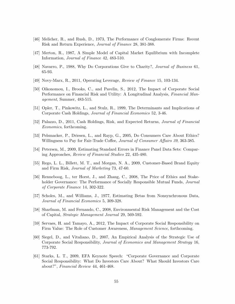
[46] Melicher, R., and Rush, D., 1973, The Performance of Conglomerate Firms: RecentRisk and Return Experience, Journal of Finance 28, 381-388.
[47] Merton, R., 1987, A Simple Model of Capital Market Equilibrium with IncompleteInformation, Journal of Finance 42, 483-510.
[48] Navarro, P., 1988, Why Do Corporations Give to Charity?, Journal of Business 61,65-93.
[49] Novy-Marx, R., 2011, Operating Leverage, Review of Finance 15, 103-134.
[50] Oikonomou, I., Brooks, C., and Pavelin, S., 2012, The Impact of Corporate SocialPerformance on Financial Risk and Utility: A Longitudinal Analysis, Financial Man-agement, Summer, 483-515.
[51] Opler, T., Pinkowitz, L., and Stulz, R., 1999, The Determinants and Implications ofCorporate Cash Holdings, Journal of Financial Economics 52, 3-46.
[52] Palazzo, D., 2011, Cash Holdings, Risk, and Expected Returns, Journal of FinancialEconomics, forthcoming.
[53] Pelsmacker, P., Driesen, L., and Rayp, G., 2005, Do Consumers Care About Ethics?Willingness to Pay for Fair-Trade Co§ee, Journal of Consumer A§airs 39, 363-385.
[54] Petersen, M., 2009, Estimating Standard Errors in Finance Panel Data Sets: Compar-ing Approaches, Review of Financial Studies 22, 435-480.
[55] Rego, L. L., Billett, M. T., and Morgan, N. A., 2009, Customer-Based Brand Equityand Firm Risk, Journal of Marketing 73, 47-60.
[56] Renneboog, L., ter Horst, J., and Zhang, C., 2008, The Price of Ethics and Stake-holder Governance: The Performance of Socially Responsible Mutual Funds, Journalof Corporate Finance 14, 302-322.
[57] Scholes, M., and Williams, J., 1977, Estimating Betas from Nonsynchronous Data,Journal of Financial Economics 5, 309-328.
[58] Sharfman, M. and Fernando, C., 2008, Environmental Risk Management and the Costof Capital, Strategic Management Journal 29, 569-592.
[59] Servaes, H. and Tamayo, A., 2012, The Impact of Corporate Social Responsibility onFirm Value: The Role of Customer Awareness, Management Science, forthcoming.
[60] Siegel, D., and Vitaliano, D., 2007, An Empirical Analysis of the Strategic Use ofCorporate Social Responsibility, Journal of Economics and Management Strategy 16,773-792.
[61] Starks, L. T., 2009, EFA Keynote Speech: “Corporate Governance and CorporateSocial Responsibility: What Do Investors Care About? What Should Investors Careabout?”, Financial Review 44, 461-468.
55

[62] Webb, N. J., 1996, Corporate Profits and Social Responsibility: “Subsidization” of Cor-porate Income Under Charitable Giving Tax Laws, Journal of Economics and Business48, 401-421.
56

!57!
Table A.I. Variables, definitions, and sources. This table presents the variable definitions and sources of data. Compustat and CRSP items are in brackets.
Variable
Definition Source
Corporate Social Responsibility
MSCI’s ESG ratings
Aggregate CSR
It is the sum of the following CSR attributes: community, diversity, employee, environment, product, and human, all defined below. It is measured annually from 2003 through 2011.
Community
It is the difference between community strengths and weaknesses. Community lists 3 concerns (investment, economic impact, and tax disputes) and 7 strengths (charitable giving, innovative giving, support for housing, support for education, non-US charitable giving, volunteer programs, and community engagement). It is measured annually from 2003 through 2011.
Diversity
It is the difference between diversity strengths and weaknesses. Diversity has 3 concerns (controversies, non-representation, and board diversity) and 8 strengths (CEO quality, promotion, board of directors, work-life benefits, women and minority contracting, employment of disabled, gay and lesbian policies, and underrepresented groups). It is measured annually from 2003 through 2011.
Employee
It is the difference between employee relations strengths and weaknesses. Employee relations has 5 concerns (union relations, health concerns, workforce reductions, retirement benefits, and supply chain) and 7 strengths (union relations, no-layoff policy, profits sharing, employee involvement, retirement benefits, health and safety, and supply chain policies). It is measured annually from 2003 through 2011.
Environment
It is the difference between environment strengths and weaknesses. Environment lists 9 concerns (waste, regulatory problems, ozone issues, emissions, agriculture chemicals, climate change, negative impact of product, biodiversity, and non-carbon releases) and 6 strengths (beneficial product, pollution prevention, recycling, clean energy, impact of property, and management system). It is measured annually from 2003 through 2011.
Product
It is the difference between product strengths and weaknesses. Product has 3 concerns (product safety, marketing concerns, and antitrust) and 4 strengths (quality, innovation, benefits to economically disadvantaged, and access to capital). It is measured annually from 2003 through 2011.
Human
It is the difference between human relations strengths and weaknesses. Human rights has 7 concerns (South Africa, Northern Ireland, Burma, Mexico, Sudan, labor rights, and indigenous people relations) and 3 strengths (South Africa, indigenous people relations, and labor rights strength). It is measured annually from 2003 through 2011.
Governance
It is the difference between governance strengths and weaknesses. Governance lists 7 concerns (high compensation, ownership, accounting, transparency, political accountability, public policy, and governance structure) and 5 strengths (limited compensation, ownership structure, transparency, political accountability, and public policy). It is measured annually from 2003 through 2011.
Sin dummy
This is a dummy variable that takes the value of one if a firm is involved in a controlversial business issue, and zero otherwise. Controlversial business issues are: firearms, gambling, military, nuclear, tobacco, and alcohol. Firearms concerns include producer of civilian arms, forearms retailer or distributor, ownership of a firearms company, ownership by a firearms company. Gambling concerns include operations, support, licensor, ownership of a gambling company, ownership by a gambling company. Military concerns include weapon systems, support systems, ownership of a military company, ownership by a military company. Nuclear concerns include builders and designers, suppliers, consulting, uranium mining, distributors, repairs. Tobacco concerns include licensor, producer, distributor, retailer, supplier, ownership of a tobacco company, ownership by a tobacco company. Alcohol concerns include producer, distributor, retailer, licensor, supplier, ownership of an alcohol company, ownership by an alcohol company. It is measured annually from 2003 through 2011.
Firm and Industry Variables Firm β
It is defined as the average value of estimation coefficients on market return and lagged market return in the regression of firm weekly excess return on market excess return, lagged market excess return, and the SMB and HML Fama-French factors. Each regression contains 52 observations. It is measured annually from 2004 through 2012.
CRSP
Tobin’s Q
It is measured as the ratio of the market value of equity (fiscal year-end price [PRCC_F] times number of shares outstanding [CSHO]) plus book value of debt (total assets [AT] less book value of equity [CEQ]) to total assets [AT]. It is measured annually from 2004 through 2012.
Compustat
Ratio of CSR firm profits to non-CSR firm profits
It is measured at the two-digit SIC industry level as mean net income [IB] of the firms in the top-third CSR score divided by the mean net income of the firms in the bottom-third CSR score. It is measured annually from 2004 through 2012.
R&D It is defined as R&D expenditure [XRD] over total assets [AT]. It is measured annually from 2003 through 2011. Advertising It is defined as advertising expenditures [XAD] over total assets [AT]. It is measured annually from 2003 through 2011.
Leverage It is defined as long-term debt [DLTT] over total assets [AT]. It is measured annually from 2003 through 2011. CAPEX It is defined as capital expenditures [CAPX] over total assets [AT]. It is measured annually from 2003 through 2011.
Cash
It is defined as the ratio of cash and marketable securities [CHE] to total assets [AT] net of cash and marketable securities (Opler et al., 1999). It is measured annually from 2003 through 2011.

!58!
Sales growth It is defined as annual growth in sales [SALE]. It is measured annually from 2003 through 2011. Compustat
ME It is the sum of the market value of equity ([PRCC_F] ×[CSHO]) over total assets [AT]. It is measured annually from 2003 through 2011. Size It is defined as the log of total assets [AT]. It is measured annually from 2003 through 2011.
Dividend yield It is defined as the dividend [DVC] per share [CSHO] over fiscal year-end price [PRCC_F]. It is measured annually from 2003 through 2011. Age It is measured as the log of the number of years since IPO. It is measured annually from 2003 through 2011.
Earnings variability It is defined as the standard deviation of earnings [IB] per share [CSHO] using a five-year rolling window. It is measured annually from 2003 through 2011.
Diversification It is measured as the number of three-digit SIC industries a firm operates in. It is measured annually from 2003 through 2011. Operating leverage
We follow Kahl et al. (2012) in measuring operating leverage. Operating leverage is measured as the sensitivity of growth in total operating costs to growth in sales. To calculate the measure, for every firm and year, we calculate ex-ante expectations of operating costs [XOPR] and sales [SALE] based on the geometric growth rate over the previous two years. Then, we generate the innovations to the growth rates. Operating leverage is -1 multiplied by the regression coefficient of the time-series regression of innovations in growth rates of operating costs on innovations in growth rates of sales. It is measured annually from 2003 through 2011.
Hoberg&Phillips product similarity
For every firm, Hoberg and Phillips (2010) perform a textual analysis of parts of 10K where companies describe their products. For every possible pair of firms i and j in Compustat, they form a vector of words describing the products and derive their similarity index. This measure is then aggregated for every firm across all other possible competitors. Larger values of this index indicate greater product similarity. The original index is divided by 10,000. It is measured annually from 2003 through 2008.
Hoberg and Phillips data website, http://www.rhsmith.umd.edu/industrydata.htm. See Hoberg and Phillips (2010) for more details.
Differentiated good industry
This dummy takes the value of 1 if the firm is in industries defined in Giannetti et al. (2011) as differentiated-product industries, and zero otherwise. The differentiated-product industries are: furniture and fixture; printing and publishing; rubber and plastic products; stone, glass, and clay products; fabricated metal products; machinery; electrical equipment; transportation equipment; instruments; miscellaneous products.
Giannetti et al. (2011)
Industry top-CSR market capitalization
Industry top-CSR market capitalization is defined at the two-digit SIC industry as market share [PRC×SHROUT] of top-third CSR firms relative to industry total market share. It is measured annually from 2003 through 2011. CRSP
GDP growth rate
It is measures as GDP growth expressed in 2003 dollars. It is measured annually from 2003 through 2011. World Bank’s World Development Indicators
Instrumental Variables President vote, democrats
This variable is the proportion of votes in the state received by the Democratic candidate for president. It is measured annually from 2003 through 2011. Stateline database
(http://www.stateline.org) and the CQ Electronic Library (http://library.cqpress.com).
Congress, democrat
It is equal to 0.5 x proportion of Senators who are Democrats + 0.5 x proportion of Congressmen who are Democrats from a particular state. It is measured annually from 2003 through 2011.
State government, democrat
It is equal to 0.5 x dummy if a governor is Democrat + 0.25 x dummy if upper Chamber is controlled by Democrats + 0.25 x dummy if lower Chamber is controlled by Democrats. It is measured annually from 2003 through 2011.
Disasters
This variable takes the value of one for a two-digit SIC industry that experienced a disaster in a given year, and zero otherwise. We obtain data on environmental and engineering disasters. Except for the oil and nuclear leakages, we include only those disasters that resulted in at least 1 death. There is a total of 53 disasters in our sample years. The type of disasters we consider include oil spills (26), nuclear leakages (6), mine accidents (3), air carrier crashes (3), train (and other transportation) accidents (4), shipwrecks (2), structural failures (3), industrial explosions (2), fires (3), and building collapses (1). The total number of deaths is 423. To differentiate events by their impact, we weight each disaster by the number of deaths. Because there were no deaths in the oil and nuclear accidents, we conservatively assign the death toll in each of these events to equal one death. It is measured annually from 2002 through 2010.
Center for Research on the Epidemiology of Disasters and newspaper articles from the Lexis-Nexis Database.
Product recalls
This variable takes the value of one for companies whose product was recalled in a given year, and zero otherwise. We consider those recalls that were covered in at least one newspaper article. For the entire sample of 4,462 companies we identify 922 product recalls for 726 companies. To assign a greater weight to more important recalls, we weight each recall by the number of newspaper articles coverage during the five days subsequent to each event. If more than one disaster occurs in an industry, or recall in a firm, in one year, we add the weights from each incident, respectively. It is measured annually from 2002 through 2010.
U.S. Consumer Product Safety Commission and newspaper articles from the Lexis-Nexis Database.
!

!
59!
Table I. Summary Statistics for Corporate Social Responsibility This table presents summary statistics for social responsibility data obtained from MSCI ESG (environment, social, governance), formerly KLD Research & Analytics. The sample years are from 2003 through 2011. The aggregate corporate social responsibility (CSR) score is the sum of six attributes: community, diversity, employee relations, environment, product, and human rights. We exclude governance from the aggregate score calculation. Appendix C provides details on the attributes and aggregate CSR score. Panel A reports summary statistics for CSR attributes and aggregate CSR score. Panel B reports the means for aggregate CSR score and its attributes by year. Panel C reports summary statistics for aggregate CSR score by one-digit SIC codes.
Panel A: Corporate Social Responsibility and its attributes !
Variable(Firm+years(((2003+2011)( Mean( Std.(dev.( Min( 25%( Median( 75%( Max(
CSR! 23,803! ,0.362! 2.162! ,9! ,2! ,1! 0! 18!Community! 23,803! !0.051! 0.486! ,2! 0! 0! 0! 5!
Diversity! 23,803! ,0.038! 1.377! ,3! ,1! 0! 1! 7!Employee! 23,803! ,0.193! 0.792! ,4! ,1! 0! 0! 5!
Environment! 23,803! 0.009! 0.715! ,5! 0! 0! 0! 5!Product! 23,803! ,0.151! 0.560! ,4! 0! 0! 0! 2!Human! 23,803! ,0.039! 0.228! ,3! 0! 0! 0! 1!
Governance! 23,803! ,0.261! 0.747! ,4! ,1! 0! 1! 2!!Panel B: Distribution by years
Year( Firm+years(( CSR( Community( Diversity( Employee(Environ+ment( Product( Human(
Gover+nance(
2003! 2,565! ,0.181! 0.043! 0.206! ,0.163! ,0.071! ,0.138! ,0.059! ,0.005!2004! 2,583! ,0.362! 0.053! 0.170! ,0.241! ,0.110! ,0.142! ,0.092! ,0.119!2005! 2,599! ,0.339! 0.036! 0.190! ,0.271! ,0.091! ,0.164! ,0.040! ,0.160!2006! 2,588! ,0.362! 0.039! 0.181! ,0.281! ,0.086! ,0.176! ,0.039! ,0.240!2007! 2,560! ,0.338! 0.017! 0.198! ,0.241! ,0.077! ,0.192! ,0.043! ,0.257!2008! 2,673! ,0.332! 0.006! 0.176! ,0.230! ,0.056! ,0.187! ,0.041! ,0.248!2009! 2,712! ,0.357! 0.001! 0.173! ,0.246! ,0.057! ,0.189! ,0.038! ,0.233!2010! 2,803! ,0.616! 0.120! ,0.797! ,0.068! 0.278! ,0.142! ,0.006! ,0.220!2011! 2,720! ,0.347! 0.135! ,0.752! ,0.014! 0.312! ,0.033! 0.006! ,0.842!Total! 23,803!
! ! ! ! ! ! ! !!Panel C: Distribution by industries
SIC(code( Industry(Firm+years((
%(of(sample(
CSR(mean(
CSR(std.(dev.(
CSR(min(
CSR(max(
100,900! Agriculture!and!Fishing! 63! 0.26%! ,1.651! 2.178! ,8! 3!1000,1700! Mining!and!Construction! 1,278! 5.37%! ,1.409! 1.768! ,9! 5!2000,2900! Manufacturing!I! 3,418! 14.36%! ,0.235! 2.636! ,8! 16!3000,3900! Manufacturing!II! 5,658! 23.77%! ,0.309! 2.269! ,8! 18!4000,4900! Transportation!and!Utilities! 2,223! 9.34%! ,0.695! 2.085! ,9! 9!5000,5900! Wholesale!Trade!and!Retail!Trade! 2,201! 9.25%! ,0.396! 2.088! ,7! 12!6000,6700! Finance,!Insurance,!and!Real!Estate! 5,294! 22.24%! ,0.162! 1.822! ,6! 14!7000,7900! Services!I! 2,748! 11.54%! ,0.107! 2.139! ,5! 14!8000,8900! Services!II! 883! 3.71%! ,0.639! 1.533! ,5! 9!9000,9900! Public!Administration! 37! 0.16%! ,0.405! 3.227! ,6! 6!
Total(!
23,803! 100.00%!! ! ! !

!
60!
Table II. Correlation Coefficients Between CSR Attributes !This table presents correlation coefficients between aggregate CSR score, its attributes, and the sin dummy variable. The attributes are community, diversity, employee relations, environment, product, and human rights. We also include the attribute governance, which is not part of the aggregate CSR score. The sample years are from 2003 through 2011. The sin dummy variable takes the value of one if a firm has one of the sin concerns and 0 otherwise. The concern categories are: firearms, gambling, military, nuclear, tobacco, and alcohol. Appendix C provides details on the attributes, aggregate CSR score and sin dummy. The numbers in parentheses are probability levels at which the hypothesis of a zero correlation can be rejected. The superscripts *, **, *** indicate significance at the 10%, 5%, and 1% levels, respectively.
!
!Sin( Community( Diversity( Employee(
Environ+ment( Product( Human(
Gover+nance(
Community( ,0.026***! ! ! ! ! ! ! !( (0.00)! ! ! ! ! ! ! !
Diversity( 0.064***! 0.287***!! ! ! ! ! !
((0.00)! (0.00)!
! ! ! ! ! !Employee( ,0.028***! 0.113***! 0.082***!! ! ! ! !
((0.00)! (0.00)! (0.00)!
! ! ! ! !Environment( ,0.120***! 0.274***! 0.146***! 0.100***!! ! ! !
((0.00)! (0.00)! (0.00)! (0.00)!
! ! ! !Product( ,0.120***! ,0.068***! ,0.211***! 0.067***! 0.082***!! ! !
((0.00)! (0.00)! (0.00)! (0.00)! (0.00)!
! ! !Human( ,0.087***! ,0.004! ,0.109***! 0.056***! 0.144***! 0.155***!! !
((0.00)! (0.50)! (0.00)! (0.00)! (0.00)! (0.00)!
! !Governance( ,0.019***! ,0.003! ,0.0220***! ,0.002! 0.075***! 0.153***! 0.082***!!
((0.00)! (0.63)! (0.00)! (0.79)! (0.00)! (0.00)! (0.00)!
!CSR( ,0.055***! 0.521***! 0.713***! 0.500***! 0.558***! 0.177***! 0.143***! 0.058***!
((0.00)! (0.00)! (0.00)! (0.00)! (0.00)! (0.00)! (0.00)! (0.00)!
!!!! !

!
61!
Table III. Summary Statistics of Main Variables This table presents summary statistics (mean, standard deviation, minimum, 25th, 50th (median) and 75th percentiles and maximum) for the main variables. The sample is the merged set between COMPUSTAT, CRSP, and MSCI ESG (environment, social, governance) formerly KLD Research & Analytics. Appendix C provides details on the definition of the variables. The sample years are from 2004 through 2012 for Firm β and Tobin’s Q, and from 2003 through 2011 for all other variables (independent variables are lagged with respect to the dependent variables). All variables, except for aggregate CSR score, are winsorized at the 1% and 99% levels.
Variable(
Firm+years( Mean( Std.(dev.( Min( 25%( Median( 75%( Max(
Firm!β! 23,803! 0.914! 0.409! 0.168! 0.572! 0.917! 1.212! 2.205!Tobin’s!Q! 23,803! 1.927! 1.419! 0.524! 1.114! 1.442! 2.215! 10.020!
CSR! 23,803! ,0.362! 2.162! ,9! ,2! ,1! 0! 18!R&D! 23,803! 0.035! 0.076! 0.000! 0.000! 0.000! 0.031! 0.455!
Advertising! 23,803! 0.009! 0.027! 0.000! 0.000! 0.000! 0.004! 0.175!Leverage! 23,803! 0.189! 0.202! 0.000! 0.010! 0.132! 0.301! 0.899!
CAPEX! 23,803! 0.041! 0.054! 0.000! 0.008! 0.024! 0.053! 0.307!Cash! 23,803! 0.482! 1.625! 0.000! 0.031! 0.100! 0.335! 5.474!
Sales!growth! 23,803! 0.158! 0.483! ,0.734! ,0.006! 0.086! 0.209! 5.462!ME! 23,803! 1.293! 1.310! 0.037! 0.430! 0.895! 1.655! 7.111!Size! 23,803! 7.232! 1.703! 3.676! 5.996! 7.117! 8.286! 11.964!
Dividend!yield,!%! 23,803! 1.416! 2.500! 0.000! 0.000! 0.000! 1.994! 15.270!Age! 23,803! 2.303! 0.884! 0.000! 1.609! 2.302! 2.639! 3.912!
Earnings!variability! 23,803! 2.302! 0.347! 0.332! 0.447! 2.412! 7.816! 37.559!Diversification! 23,803! 4.260! 0.450! 1.000! 2.000! 4.000! 5.000! 16.000!
Operating!leverage! 23,803! -0.986! 3.694! ,6.440! ,0.690! ,0.990! ,0.280! 4.290!Hoberg&Phillips!product!similarity! 15,001! 0.0773! 0.143! 0.010! 0.128! 0.216! 0.501! 10.001!

!
62!
Table IV. Panel Regressions of Firm β on CSR and Its Attributes with Firm Fixed Effects and Year Fixed Effects! This table reports the results of panel regressions of Firm β on aggregate CSR score (governance excluded) and its attributes (community, diversity, employee relations, environment, product, and human rights). Specification 9 includes governance in the CSR score calculation. Specification 11 controls for the sin dummy. The regressions are run using the panel of firm-year observations from 2003 through 2012. All independent variables are lagged by one year. Every regression includes firm and year fixed effects. Standard errors are clustered by firms and years to adjust for arbitrary heteroskedasticity, cross-sectional, and time-series correlation. The numbers in parentheses are t-statistics. The superscripts *, **, *** indicate significance at the 10%, 5%, and 1% levels, respectively. All variables except for CSR are winsorized at the 1% and 99% levels. Appendix C contains a detailed description of all the variables.
Specification+ 1+ 2+ 3+ 4+ 5+ 6+ 7+ 8+ 9+ 10+ 11+
Dependent+variable+ Firm%β%
lagged!CSR! )0.0168***!
! ! ! ! ! ! ! ! !)0.0152***!
!()6.14)!
! ! ! ! ! ! ! ! !()5.71)!
lagged!Community!!
)0.0321***!! ! ! ! ! ! ! ! !
! !()3.15)!
! ! ! ! ! ! ! ! !lagged!Diversity!! !
)0.0199***!! ! ! ! ! ! ! !
! ! !()3.41)!
! ! ! ! ! ! ! !lagged!Employee!! ! !
)0.0155**!! ! ! ! ! ! !
! ! ! !()2.32)!
! ! ! ! ! ! !lagged!Environment!! ! ! !
)0.0312***!! ! ! ! ! !
! ! ! ! !()6.92)!
! ! ! ! ! !lagged+Product!! ! ! ! !
0.0020!! ! ! ! !
! ! ! ! ! !(0.24)!
! ! ! ! !lagged!Human!! ! ! ! ! !
)0.0842***!! ! ! !
! ! ! ! ! ! !()4.42)!
! ! ! !lagged!Governance!! ! ! ! ! ! !
0.0036!! ! !
! ! ! ! ! ! ! !(0.63)!
! ! !lagged!CSR+(with+Gov.)!! ! ! ! ! ! ! !
)0.0115***!! !
! ! ! ! ! ! ! ! !()5.09)!
! !lagged!Sin+dummy!! ! ! ! ! ! ! ! !
0.0350! 0.0212!
! ! ! ! ! ! ! ! ! !(1.48)! (0.93)!
Number!of!firm)years! 23,803! 23,803! 23,803! 23,803! 23,803! 23,803! 23,803! 23,803! 23,803! 23,803! 23,803!
R2! 0.537! 0.537! 0.537! 0.537! 0.537! 0.536! 0.537! 0.536! 0.538! 0.536! 0.537!!

!
63!
Table V. Panel Regressions of Firm β on CSR and Its Attributes with Control Variables, Firm Fixed Effects and Year Fixed Effects!
This table reports the results of panel regressions of Firm β on aggregate CSR score (governance excluded), its attributes (community, diversity, employee relations, environment, product, and human rights) and other controls. Specification 10 includes governance in the CSR score calculation. Specification 11 controls for the sin dummy. The regressions are run using the panel of firm-year observations from 2003 through 2012. All independent variables are lagged by one year. Every regression includes firm and year fixed effects. Standard errors are clustered by firms and years to adjust for arbitrary heteroskedasticity, cross-sectional, and time-series correlation. The numbers in parentheses are t-statistics. The superscripts *, **, *** indicate significance at the 10%, 5%, and 1% levels, respectively. All variables except for CSR are winsorized at the 1% and 99% levels. Appendix C contains a detailed description of all the variables.

!
64!
Specification+ 1+ 2+ 3+ 4+ 5+ 6+ 7+ 8+ 9+ 10+ 11+
Dependent+variable++ Firm%β%CSR!variable!included!in!the!
regression!! ! CSR! Community! Diversity! Employee! Environment! Product! Human! Governance!CSR+(with+Gov.)! CSR!
lagged!CSR+variable!!
70.0158***! 70.0312***! 70.0271***! 70.0129**! 70.0317***! 0.0027! 70.0769***! 0.0032! 70.0114***! 70.0150***!
! !(76.47)! (73.35)! (73.94)! (72.38)! (75.84)! (0.20)! (74.33)! (0.59)! (75.47)! (76.32)!
lagged!Sin+dummy!! ! ! ! ! ! ! ! ! !
0.0282!
! ! ! ! ! ! ! ! ! ! !(1.20)!
lagged+Operating+leverage+ 0.0063! 0.0045! 0.0050! 0.0055! 0.0049! 0.0045! 0.0051! 0.049! 0.0054! 0.0049! 0.0045!
! (0.92)! (0.69)! (0.77)! (0.84)! (0.75)! (0.69)! (0.78)! (0.75)! (0.82)! (0.74)! (0.77)!
lagged!R&D! 70.4990***! 70.4554***! 70.4621***! 70.4628***! 70.4672***! 70.4737***! 70.4620***! 70.4685***! 70.4667***! 70.4730***! 70.4742***!
!(73.62)! (73.58)! (73.50)! (73.47)! (73.42)! (73.45)! (73.52)! (73.57)! (73.60)! (73.54)! (73.46)!
lagged!Advertising! 70.0402! 70.0120! 70.0234! 70.0308! 70.0326! 70.0217! 70.0282! 70.0284! 70.0219! 70.0192! 70.0176!
!(70.30)! (70.12)! (70.14)! (70.16)! (70.12)! (70.19)! (70.14)! (70.13)! (70.18)! (70.15)! (70.10)!
lagged!Leverage! 0.2717***! 0.2386***! 0.2312***! 0.2440***! 0.2380***! 0.2428***! 0.2375***! 0.2329***! 0.2314***! 0.2289***! 0.2620***!
!(4.39)! (4.35)! (4.37)! (4.21)! (4.24)! (4.25)! (4.32)! (4.36)! (4.17)! (4.29)! (4.20)!
lagged!CAPEX! 70.0714! 70.0913! 70.0920! 70.0968! 70.1000! 70.1014! 70.1021! 70.1117! 70.1102! 70.1152! 70.1019!
!(70.48)! (70.58)! (70.60)! (70.62)! (70.58)! (70.77)! (70.73)! (70.70)! (70.62)! (70.62)! (70.67)!
lagged!Cash! 0.2214***! 0.1915***! 0.1988***! 0.2014***! 0.2157***! 0.2072***! 0.1929***! 0.1921***! 0.1968***! 0.2081***! 0.2005***!
!(3.85)! (3.20)! (3.27)! (3.20)! (4.14)! (3.97)! (3.94)! (3.59)! (3.62)! (3.65)! (3.90)!
lagged!Sales+growth! 0.0071! 0.0082! 0.0070! 0.0089! 0.0162! 0.0150! 0.0155! 0.0094! 0.0092! 0.0088! 0.0099!
!(1.26)! (1.31)! (1.30)! (1.42)! (1.20)! (1.26)! (1.24)! (1.21)! (1.15)! (1.20)! (1.14)!
lagged!ME! 0.0513***! 0.0451***! 0.0482***! 0.0416***! 0.0421***! 0.0390***! 0.0422***! 0.0488***! 0.0484***! 0.0479***! 0.0522***!
!(7.62)! (7.44)! (7.41)! (7.40)! (7.34)! (7.30)! (7.27)! (7.21)! (7.16)! (8.02)! (7.20)!
lagged!Size! 0.0087! 0.0096! 0.0065! 0.0069! 0.0108! 0.0136! 0.0182! 0.0146! 0.0146! 0.0139! 0.0171!
!(0.65)! (0.47)! (0.49)! (0.42)! (0.48)! (0.651! (0.57)! (0.52)! (0.55)! (0.64)! (0.57)!
lagged!Dividend+yield! 0.2940**! 0.244**! 0.2939**! 0.2937**! 0.2942**! 0.2944**! 0.2817**! 0.2851**! 0.2903**! 0.3014**! 0.2848**!
!(2.37)! (2.48)! (2.43)! (2.40)! (2.28)! (2.39)! (2.47)! (2.41)! (2.32)! (2.43)! (2.30)!
lagged!Age!! 0.0084! 0.0130! 0.0054! 0.0007! 0.0050! 0.0040! 0.0069! 0.0078! 0.0074! 0.0139! 0.0214!
!(0.68)! (0.69)! (0.65)! (0.53)! (0.59)! (0.52)! (0.42)! (0.44)! (0.64)! (0.67)! (0.53)!
lagged!Earnings+variability! 0.0121! 0.0202! 0.0186! 0.0107! 0.0185! 0.0141! 0.0216! 0.0249! 0.0163! 0.0249! 0.0283!
!(0.21)! (0.17)! (0.19)! (0.19)! (0.18)! (0.17)! (0.18)! (0.20)! (0.20)! (0.21)! (0.22)!
lagged!Diversification! 0.0076***! 0.0072***! 0.0064***! 0.0049***! 0.0052***! 0.0054***! 0.0058***! 0.0079***! 0.0070***! 0.0014***! 0.0122***!
!(3.12)! (3.16)! (3.12)! (3.07)! (3.12)! (3.17)! (3.05)! (3.17)! (3.21)! (3.07)! (3.19)!
Number!of!firm7years! 23,803! 23,803! 23,803! 23,803! 23,803! 23,803! 23,803! 23,803! 23,803! 23,803! 23,803!
R2! 0.544! 0.545! 0.544! 0.544! 0.544! 0.544! 0.544! 0.544! 0.544! 0.544! 0.545!

!
65!
Table VI. Regressions of Firm β on CSR by Year! This table reports the coefficient on aggregate CSR score in the regressions of Firm β on aggregate CSR score as in specification 1 of Table IV (in Panel A) and aggregate CSR score and controls as in specification 2 of Table V (shown in Panel B). Standard errors are adjusted for heteroskedasticity. The numbers in parentheses are t-statistics. The superscripts *, **, *** indicate significance at the 10%, 5%, and 1% levels, respectively. !
!
Panel&A:&Specification&without&controls&
Panel&B:&Specification&with&controls&
Year& CSR& t9stat& N.Obs.& CSR& t9stat& N.Obs.&2011& !!!!$0.0208***! ($5.90)! 2,720! !!!!$0.0195***! ($4.14)! 2,720!2010& !!!!$0.0239***! ($5.22)! 2,803! !!!!$0.0198***! ($4.62)! 2,803!2009& !!!!$0.0065! ($1.18)! 2,712! !!!!!0.0023! (0.38)! 2,712!2008& !!!!$0.0212***! ($4.59)! 2,673! !!!!$0.0139***! ($3.17)! 2,673!2007& !!!!$0.0172***! ($3.70)! 2,560! !!!!$0.0166***! ($3.42)! 2,560!2006& !!!!$0.0450***! ($8.14)! 2,588! !!!!$0.0314***! ($6.58)! 2,588!2005& !!!!$0.0391***! ($6.97)! 2,599! !!!!$0.0322***! ($6.13)! 2,599!2004& !!!!$0.0362***! ($5.89)! 2,583! !!!!$0.0318***! ($5.21)! 2,583!2003& !!!!$0.0042! ($0.69)! 2,565! !!!!$0.0191**! ($2.25)! 2,565!

!
66!
Table VII. Panel Regressions of Firm β on CSR Conditional on Differentiated Goods Industry, Product Similarity, and Industry top-CSR Market Capitalization!
In specifications 1-3 we report the results of panel regressions of Firm β on aggregate CSR score (governance excluded) and interactions of CSR with Differentiated goods industry dummy variable (specification 1), Hoberg and Phillips product similarity, (specification 2), and Industry Top-CSR market capitalization (specification 3). Specification 4 reports regression of Profit ratio on GDP per capita growth and two-digit SIC industry dummies. The sample years are from 2003 through 2012 (independent variables in specifications 1-4 are lagged with respect to the dependent variables). Regressions in specifications 1-3 include all control variables as in Table V. Differentiated goods industries (24% of the sample) are taken from Giannetti, et al. (2011): furniture and fixture; printing and publishing; rubber and plastic products; stone, glass, and clay products; fabricated metal products; machinery; electrical equipment; transportation equipment; instruments; miscellaneous products. Industry top-CSR market capitalization is defined at the two-digit SIC industry as market share of top-third CSR firms relative to industry total market share. Profit ratio is defined at the two-digit SIC industry as the mean net income of the firms in the top-third CSR score divided by the mean net income of the firms in the bottom-third CSR score. Appendix C provides details on the definition of the variables. Except in specification (4), standard errors are clustered by firms and years to adjust for arbitrary heteroskedasticity, cross-sectional, and time-series correlation. The numbers in parentheses are t-statistics. Superscripts *, **, *** indicate significance at the 10%, 5%, and 1% levels, respectively. All firm variables, except for CSR, are winsorized at the 1% and 99% levels.
Specification+ 1+ 2+ 3++ 4+
Dependent+variable+ Firm%β% Profit+ratio+
lagged!CSR! (0.0181**! (0.0243***! (0.0198***! !
!((6.78)! ((5.19)! ((4.60)! !
GDP+growth+ ! ! ! (0.122***!+ ! ! ! ((6.15)!
Differentiated+goods+industry!dummy! 0.1950***! ! ! !
!(22.74)! ! ! !
Differentiated+goods+×!lagged!CSR! (0.0061***! ! ! !
!((3.08)! ! ! !
Hoberg&Phillips+similar+goods+ ! (0.2132*! ! !
!! ((1.63)! ! !
Hoberg&Phillips+similar+goods×lagged+CSR! ! 0.0981***! ! !
!! (5.14)! ! !
Industry+topDCSR+market+cap+ ! ! (0.0098**! !
!! ! ((1.75)! !
Industry+topDCSR+market+cap×lagged+CSR! ! ! !!0.0079***! !
!! ! (3.20)! !
All!control!variables!included! yes! yes! yes! no!Firm!fixed!effects! no! yes! yes! no!
Industry!fixed!effects! no! no! no! yes!Year!fixed!effects! yes! yes! yes! no!Number!of!obs.! 23,803! 15,001! 23,803! 442!
R2! 0.185! 0.594! 0.546! 0.277!!
!
67!
Table VIII. Panel Regressions of Tobin’s Q!
This table reports the results of panel regressions of Tobin’s Q on aggregate CSR score (specification 1) and interactions of firm CSR with Differentiated goods industry dummy variable (specification 2), Hoberg-Phillips product similarity (specification 3), and Industry top-CSR market capitalization (specification 4). The regressions are run using the panel of firm-year observations from 2003 through 2012. Independent variables are lagged by one year. Appendix C provides details on the definition of the variables. Specifications 1, 3, and 4 include firm and year fixed effects. Standard errors are clustered by firms and years to adjust for arbitrary heteroskedasticity, cross-sectional, and time-series correlation. The numbers in parentheses are t-statistics. The upper scripts *, **, *** indicate significance at the 10%, 5%, and 1% levels, respectively. All variables except for CSR are winsorized at the 1% and 99% levels. !
Specification+ 1+ 2+ 3+ 4+
Dependent+variable+ Tobin’s(Q+lagged!CSR! 0.0630***! 0.0487***! 0.0481***! 0.0523***!
!(9.17)! !!(8.68)! !!(5.66)! (6.39)!
Differentiated+goods+industry!dummy! ! =0.0794**! ! !
! ! (=2.03)! ! !
Differentiated+goods+×!lagged!CSR! ! 0.0253***! ! !
! ! (3.25)! ! !
Hoberg&Phillips+similar+goods! ! ! 0.2192***! !
! ! ! (6.12)! !
Hoberg&Phillips+similar+goods×lagged!CSR! ! ! =0.0801**! !
! ! ! (2.22)! !
Industry+topBCSR+market+cap.+ ! ! ! 0.0239!
! ! ! ! (0.54)!
Industry+topBCSR+mark+cap.+×lagged!CSR! ! ! ! =0.0092*!
! ! ! ! (=1.70)!
lagged!Operating+leverage! 0.0042! 0.0062! 0.0068! 0.0060!! (1.16)! (1.60)! (1.57)! (1.58)!
lagged!R&D! !!1.9040***! 4.1330***! 4.0203***! 4.1774***!! (4.07)!! (11.75)! (11.69)! (11.20)!
lagged!Advertising! 1.3536! 2.9044***! 2.7839***! 2.8023***!
!(1.32)! (3.20)! (3.29)! (3.10)!
lagged!Leverage! =0.2041**! =0.1288! =0.1142! =0.1158!
!(=1.69)! (=0.90)! (=0.88)! (=0.68)!
lagged!CAPEX! 1.3037***! 1.8227***! 1.9839***! 1.7482***!
!(4.63)! !(8.02)! (8.27)! (7.22)!
lagged!Sales+growth! 0.2178***! 0.3049***! 0.3016***! 0.3329***!
!(8.08)! !!(9.30)! (9.03)! (10.11)!
lagged!Size! =0.5663! =0.1888! =0.1839***! =0.1663***!
!(=13.13)! (=14.54)! (=14.37)! (=13.90)!
lagged!Age!! =0.1219***! =0.2709***! =0.2840***! =0.2472***!
!(4.34)! (6.21)! (6.21)! (6.42)!
lagged!Diversification! =0.0324! =0.0164! =0.03240! =0.0281!
!(=1.21)! (=1.00)! (=1.10)! (=1.29)!
Firm!fixed!effects! yes! no! yes! yes!Year!fixed!effects! yes! yes! no! yes!
Number!of!firm=years! 23,803! 23,803! 15,001! 23,803!R2! 0.581! 0.272! 0.584! 0.583!
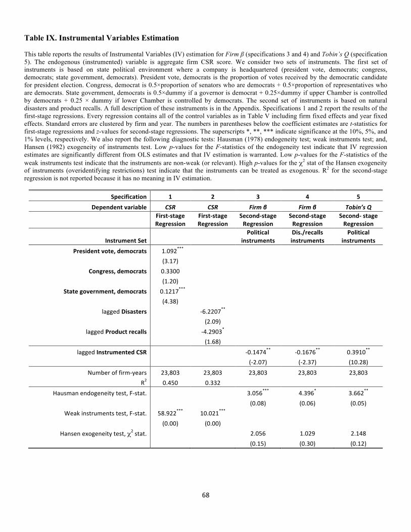
!
68!
Table IX. Instrumental Variables Estimation!
This table reports the results of Instrumental Variables (IV) estimation for Firm β (specifications 3 and 4) and Tobin’s Q (specification 5). The endogenous (instrumented) variable is aggregate firm CSR score. We consider two sets of instruments. The first set of instruments is based on state political environment where a company is headquartered (president vote, democrats; congress, democrats; state government, democrats). President vote, democrats is the proportion of votes received by the democratic candidate for president election. Congress, democrat is 0.5×proportion of senators who are democrats + 0.5×proportion of representatives who are democrats. State government, democrats is 0.5×dummy if a governor is democrat + 0.25×dummy if upper Chamber is controlled by democrats + 0.25 × dummy if lower Chamber is controlled by democrats. The second set of instruments is based on natural disasters and product recalls. A full description of these instruments is in the Appendix. Specifications 1 and 2 report the results of the first-stage regressions. Every regression contains all of the control variables as in Table V including firm fixed effects and year fixed effects. Standard errors are clustered by firm and year. The numbers in parentheses below the coefficient estimates are t-statistics for first-stage regressions and z-values for second-stage regressions. The superscripts *, **, *** indicate significance at the 10%, 5%, and 1% levels, respectively. We also report the following diagnostic tests: Hausman (1978) endogeneity test; weak instruments test; and, Hansen (1982) exogeneity of instruments test. Low p-values for the F-statistics of the endogeneity test indicate that IV regression estimates are significantly different from OLS estimates and that IV estimation is warranted. Low p-values for the F-statistics of the weak instruments test indicate that the instruments are non-weak (or relevant). High p-values for the χ2 stat of the Hansen exogeneity of instruments (overidentifying restrictions) test indicate that the instruments can be treated as exogenous. R2 for the second-stage regression is not reported because it has no meaning in IV estimation.
Specification+ 1+ 2+ 3+ 4+ 5+Dependent+variable+ CSR$ CSR$ Firm$β+ Firm$β+ Tobin’s$Q$
+First9stage+Regression+
First9stage+Regression+
Second9stage+Regression+
Second9stage+Regression+
Second9+stage+Regression+
Instrument+Set+ + +Political+
instruments+Dis./recalls+instruments+
Political+instruments+
President+vote,+democrats+ !!!1.092***! ! ! ! !! (3.17)! ! ! ! !
Congress,+democrats+ 0.3300! ! ! ! !! (1.20)! ! ! ! !
State+government,+democrats+ !!!0.1217***! ! ! ! !! (4.38)! ! ! ! !
lagged!Disasters! ! 46.2207**! ! ! !! ! (2.09)! ! ! !
lagged!Product+recalls! ! 44.2903*! ! ! !! ! (1.68)! ! ! !
lagged!Instrumented+CSR! ! ! 40.1474**! 40.1676**! 0.3910**!! ! ! (42.07)! (42.37)! (10.28)!
Number!of!firm4years! 23,803! 23,803! 23,803! 23,803! 23,803!R2! 0.450! 0.332! ! ! !
Hausman!endogeneity!test,!F4stat.! ! ! 3.056***! 4.396*! 3.662**!
! ! ! (0.08)! (0.06)! (0.05)!Weak!instruments!test,!F4stat.! 58.922***! 10.021***! ! ! !
! (0.00)! (0.00)! ! ! !Hansen!exogeneity!test,!χ2!stat.! ! ! 2.056! 1.029! 2.148!
! ! ! (0.15)! (0.30)! (0.12)!!
!
Top Related