


Languages
Pages
Legal

DIGITAL SWITCHING IN THE QUANTUM
DOMAIN
Riccardo RICCI, Francesco VITULO
A.A. 2002/03
Corso di Nanotecnologie 1

R. Ricci, F. Vitulo 2
QUANTUM STATE• Each particle has its own quantum state.
• It can be represented as a linear combination of two eigenstates: |0 and |1.
• |0 and |1 can be used to simulate the classical binary logic, so the particle is called qubit.
• A particle usually is in condition of superposition, and has a part |0 and a part |1.
• When a particle is measured, it is projected to one of its states, |0 or |1.
R. Ricci, F. Vitulo 3
QUANTUM STATE
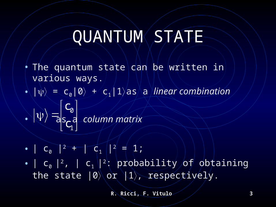
• The quantum state can be written in various ways.
• | = c0|0 + c1|1 as a linear combination
• as a column matrix
• | c0 |2 + | c1 |2 = 1;
• | c0 |2, | c1 |2: probability of obtaining the state |0 or |1, respectively.
R. Ricci, F. Vitulo 4
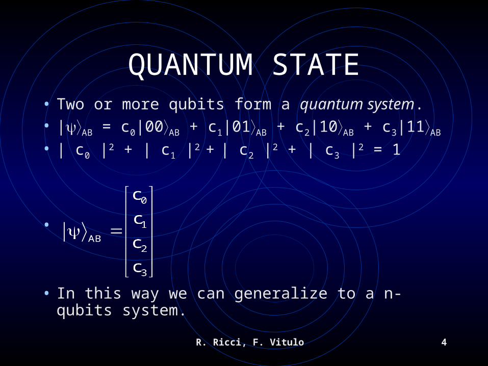
QUANTUM STATE• Two or more qubits form a quantum system.• |AB = c0|00AB + c1|01AB + c2|10AB + c3|11AB
• | c0 |2 + | c1 |2 + | c2 |2 + | c3 |2 = 1
•
• In this way we can generalize to a n-qubits system.

R. Ricci, F. Vitulo 5
QUANTUM GATE• A quantum gate manipulates a quantum system.
• It can be represented in form of a matrix operation.
• Example 1: NOT gate
• It changes the state from |0 to |1 and vice-versa.

R. Ricci, F. Vitulo 6
QUANTUM GATE• Example 2: Control-NOT (CN) gate.
• It has one control qubit and one target qubit.• Target qubit changes his state if control qubit state = |1.
R. Ricci, F. Vitulo 7
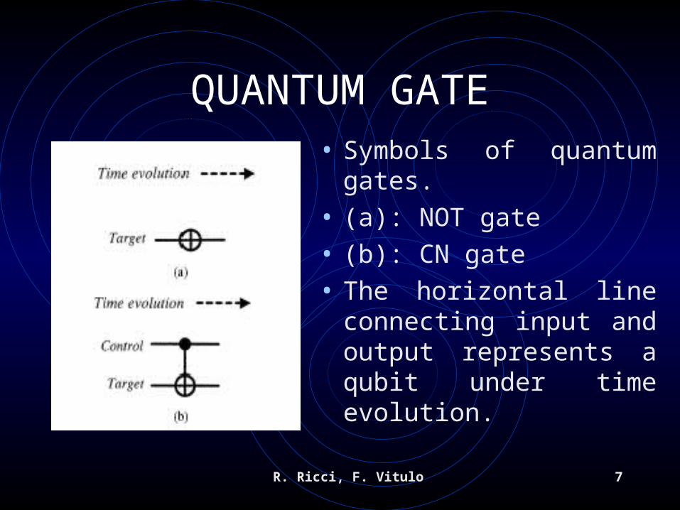
QUANTUM GATE• Symbols of quantum gates.
• (a): NOT gate
• (b): CN gate
• The horizontal line connecting input and output represents a qubit under time evolution.
R. Ricci, F. Vitulo 8
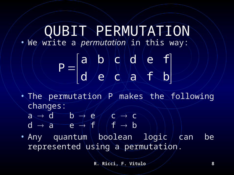
QUBIT PERMUTATION• We write a permutation in this way:
• The permutation P makes the following changes:a d b e c cd a e f f b
• Any quantum boolean logic can be represented using a permutation.
R. Ricci, F. Vitulo 9
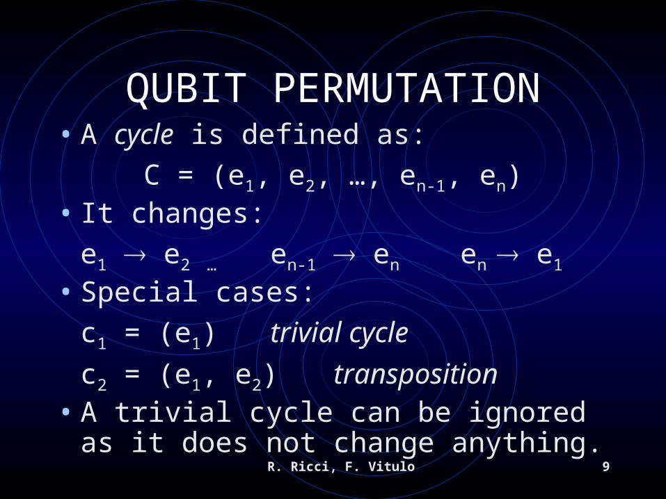
QUBIT PERMUTATION• A cycle is defined as:
C = (e1, e2, …, en-1, en)• It changes:
e1 e2 … en-1 en en e1
• Special cases:
c1 = (e1) trivial cycle
c2 = (e1, e2)transposition• A trivial cycle can be ignored as it does not
change anything.

R. Ricci, F. Vitulo 10
QUBIT PERMUTATION• A permutation can be expressed as disjoint cycles:
• P is equivalent to:
P = (a, d) (c) (b, e, f) = (a, d) (b, e, f)
• The implementation consists of executing cycles of various lenghts in parallel.

R. Ricci, F. Vitulo 11
QUBIT PERMUTATION• The transposition of two qubits can be done using
three CN gates, as shown in the picture below:
• The proof is in [1].

R. Ricci, F. Vitulo 12
IMPLEMENTATION OF CYCLES
• A n-qubit cycle C can be done by six layers of CN gates.
C = (q0, q1, …, qn-1)
• Case 1: if n is even (n = 2m), we define:
X = (qm-1, qm+1) … (q2, qn-2) (q1, qn-1)
Y = (qm, qm+1) … (q2, qn-1) (q1, q0)
• The cycle is implemented as:
U = YX

R. Ricci, F. Vitulo 13
IMPLEMENTATION OF CYCLES
• Case 2: if n is odd (n = 2m + 1), we define:
X = (qm, qm+1) … (q2, qn-2) (q1, qn-1)
Y = (qm, qm+2) … (q2, qn-1) (q1, q0)• The cycle is implemented as:
U = YX
Case 1 Case 2
R. Ricci, F. Vitulo 14
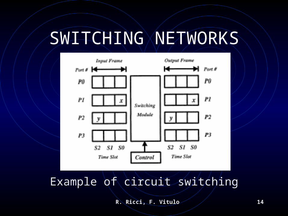
SWITCHING NETWORKS
Example of circuit switching
R. Ricci, F. Vitulo 15
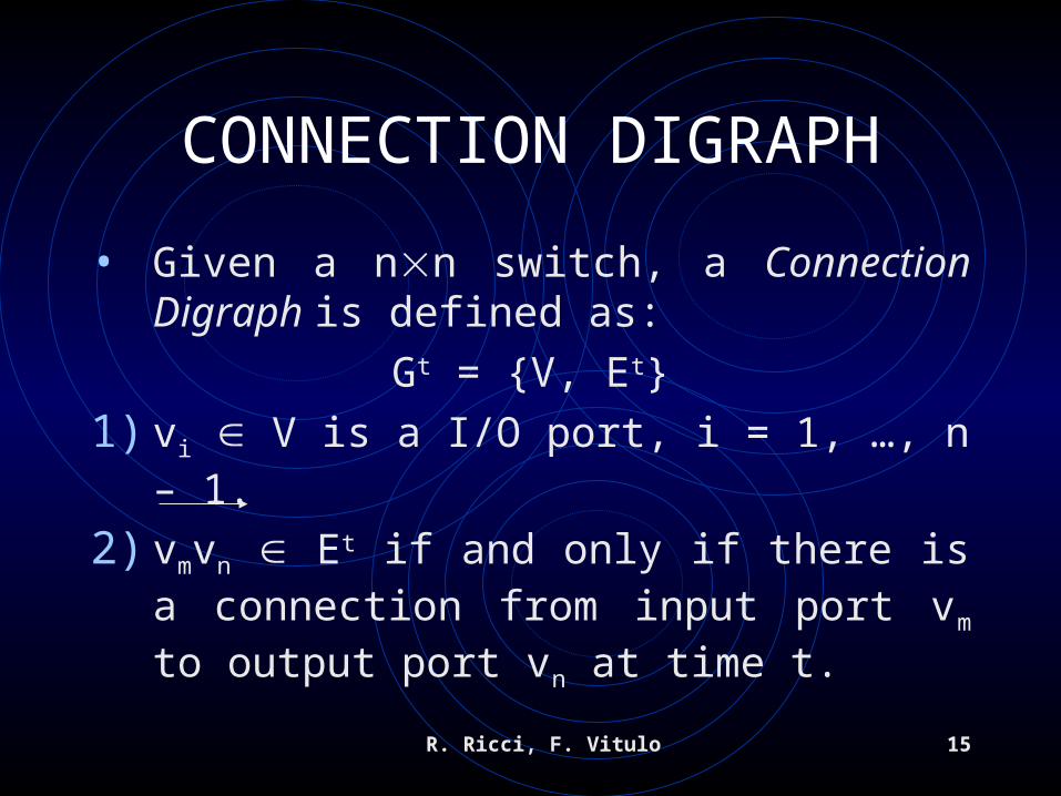
CONNECTION DIGRAPH
• Given a nn switch, a Connection Digraph is defined as:
Gt = {V, Et}
1) vi V is a I/O port, i = 1, …, n – 1.
2) vmvn Et if and only if there is a connection from input port vm to output port vn at time t.
R. Ricci, F. Vitulo 16
CONNECTION DIGRAPH
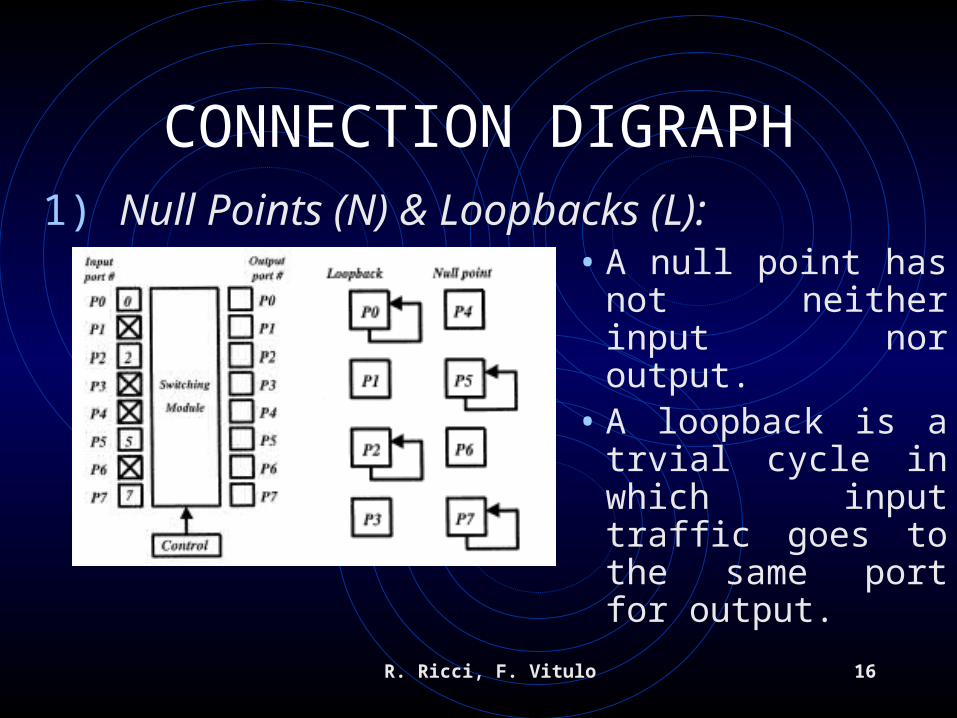
• A null point has not neither input nor output.
• A loopback is a trvial cycle in which input traffic goes to the same port for output.
1) Null Points (N) & Loopbacks (L):
R. Ricci, F. Vitulo 17
CONNECTION DIGRAPH
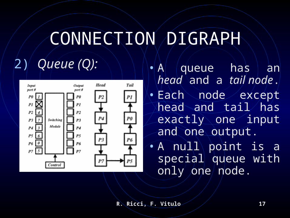
• A queue has an head and a tail node.
• Each node except head and tail has exactly one input and one output.
• A null point is a special queue with only one node.
2) Queue (Q):
R. Ricci, F. Vitulo 18
CONNECTION DIGRAPH
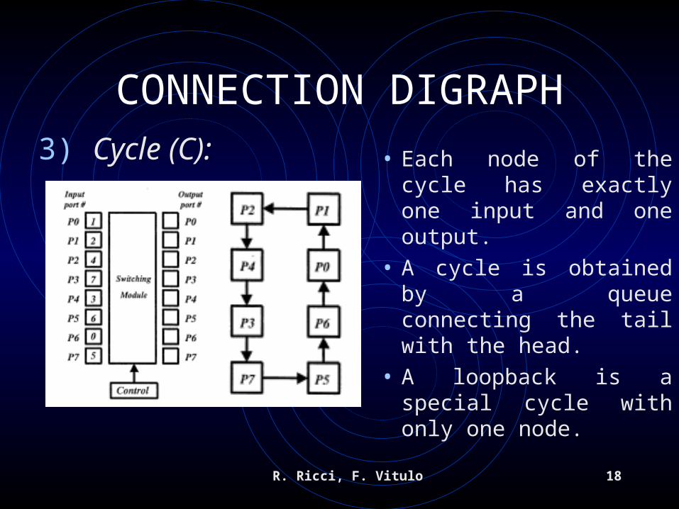
• Each node of the cycle has exactly one input and one output.
• A cycle is obtained by a queue connecting the tail with the head.
• A loopback is a special cycle with only one node.
3) Cycle (C):
R. Ricci, F. Vitulo 19
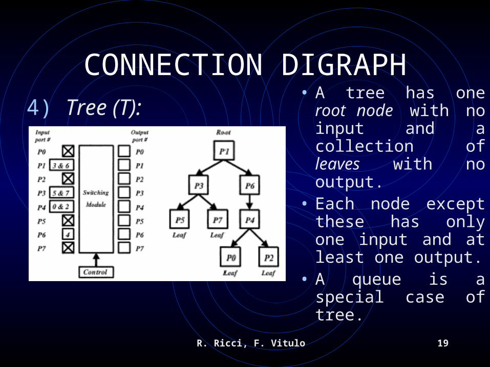
CONNECTION DIGRAPH• A tree has one root
node with no input and a collection of leaves with no output.
• Each node except these has only one input and at least one output.
• A queue is a special case of tree.
4) Tree (T):
R. Ricci, F. Vitulo 20
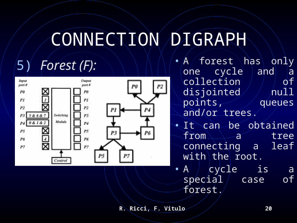
CONNECTION DIGRAPH• A forest has only one
cycle and a collection of disjointed null points, queues and/or trees.
• It can be obtained from a tree connecting a leaf with the root.
• A cycle is a special case of forest.
5) Forest (F):

R. Ricci, F. Vitulo 21
DIGITAL QUANTUM SWITCHING
R. Ricci, F. Vitulo 22
DIGITAL QUANTUM SWITCHING
• The I/O port can be either quantum or classical oriented.
• Switching can be done efficiently using CN gates.
• It can also switch classical information using C/Q converters in input and Q/C converters in output.

R. Ricci, F. Vitulo 23
DIGITAL QUANTUM SWITCHING
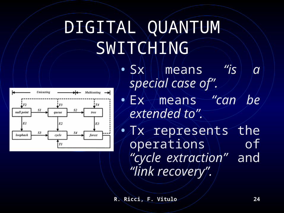
• Unicasting connection digraph is a collection of disjointed null points, loopbacks, queues and/or cycles as subdigraphs.
• Multicasting connection digraph contains trees and forests as subdigraphs.
• All these topologies are inter-related each other.
R. Ricci, F. Vitulo 24
DIGITAL QUANTUM SWITCHING
• Sx means “is a special case of”.
• Ex means “can be extended to”.
• Tx represents the operations of “cycle extraction” and “link recovery”.

R. Ricci, F. Vitulo 25
1) Cycle extraction:
DIGITAL QUANTUM SWITCHING
R. Ricci, F. Vitulo 26
1) Cycle extraction:
• It transforms a forest into one cycle and a collection of null points, queues and/or trees.
• If there are still any trees, they can be transformed in a forest and can be applied again the process of cycle extraction.
• In order to implement a connection digraph we need to transform every subdigraph into cycles or loopbacks.
DIGITAL QUANTUM SWITCHING

R. Ricci, F. Vitulo 27
DIGITAL QUANTUM SWITCHING
2) Link recovery:
R. Ricci, F. Vitulo 28
DIGITAL QUANTUM SWITCHING
2) Link recovery:
• It recovers the links that have been cut.
• All the elementary topologies can be reduced to a collection of loopbacks and cycles: this allows an efficient implementation of the switching process.
R. Ricci, F. Vitulo 29
UNICAST QUANTUM SWITCHING
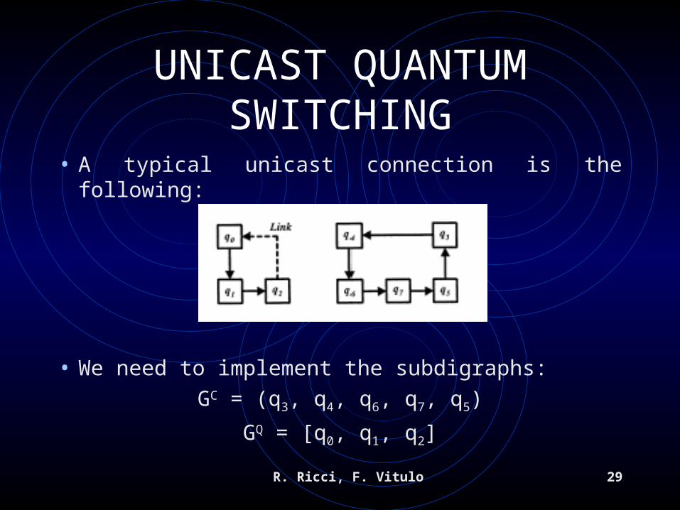
• A typical unicast connection is the following:
• We need to implement the subdigraphs:
GC = (q3, q4, q6, q7, q5)
GQ = [q0, q1, q2]
R. Ricci, F. Vitulo 30
UNICAST QUANTUM SWITCHING
• First, we extend GQ to GC’ = (q0, q1, q2).
• The subdigraph GC can be done applying:
X = (q6, q7) (q4, q5)
Y = (q6, q5) (q4, q5)
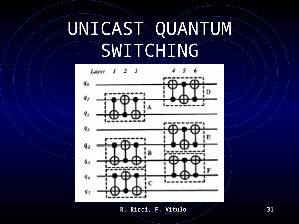
• Then, we implement GC and GC’ using six layers of CN gates (see picture on the next slide).
R. Ricci, F. Vitulo 31
UNICAST QUANTUM SWITCHING
R. Ricci, F. Vitulo 32
MULTICAST QUANTUM SWITCHING
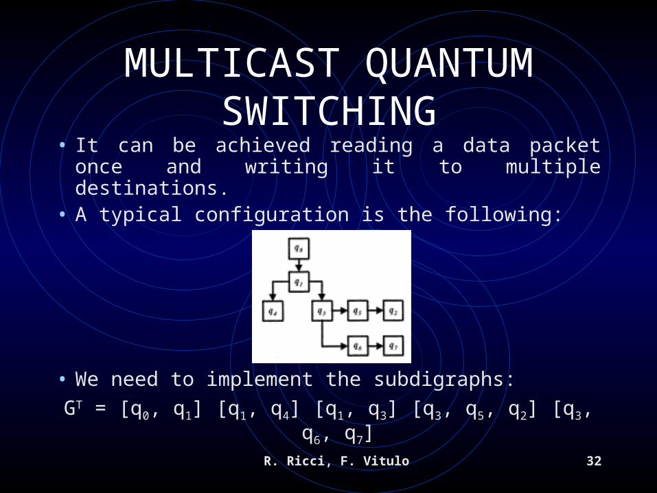
• It can be achieved reading a data packet once and writing it to multiple destinations.
• A typical configuration is the following:
• We need to implement the subdigraphs:
GT = [q0, q1] [q1, q4] [q1, q3] [q3, q5, q2] [q3, q6, q7]
R. Ricci, F. Vitulo 33
MULTICAST QUANTUM SWITCHING
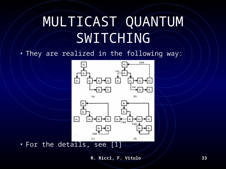
• They are realized in the following way:
• For the details, see [1]
R. Ricci, F. Vitulo 34
MULTICAST QUANTUM SWITCHING
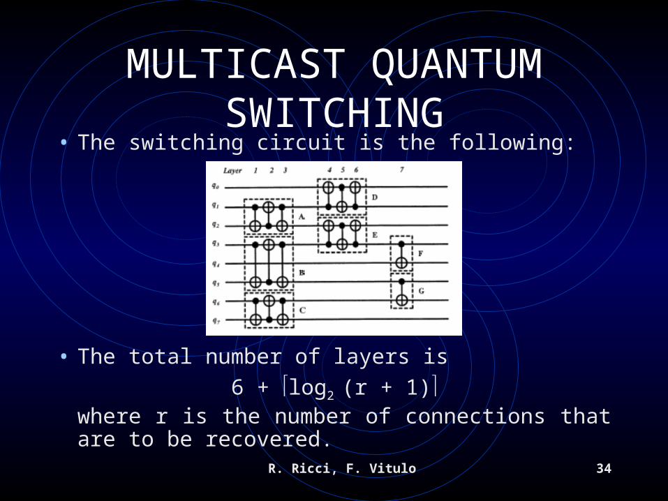
• The switching circuit is the following:
• The total number of layers is
6 + log2 (r + 1)where r is the number of connections that are to be recovered.
R. Ricci, F. Vitulo 35
ADVANTAGES OF QUANTUM SWITCHING
• Quantum switching is strict-sense non-blocking: the network can always connect each idle inlet to an arbitrary idle outlet independent of the current network permutation.
• In fact, quantum switching is a unitary transformation, which is always possible.

R. Ricci, F. Vitulo 36
ADVANTAGES OF QUANTUM SWITCHING
• Unicast quantum switching has time complexity O(1) as a space switch, because the circuit can be implemented with only six layers of CN gates, and has space complexity O(n), where n is the number of input qubits.
• Multicast quantum switching has time complexity O(log2 n) and space complexity O(n).
• These values cannot be achieved in the same time with a classical switch.
R. Ricci, F. Vitulo 37
ISSUES OF QUANTUM SWITCHING: DECOHERENCE• Decoherence is a coupling between two initially
isolated quantum systems (qubit and environment) that randomizes the relative phases of the states.
• It is the probability that quantum information spread out the computer, compromising the computation results.
• To avoid it, engineers should produce sub-micro systems in which qubits influence each other, but are completely insulated from the external environment.

R. Ricci, F. Vitulo 38
ISSUES OF QUANTUM SWITCHING: DECOHERENCE• In this case, we need to maximize:
Smax = t0 / td
where td is decoherence time and t0 is the time of a single operation.
• If 6 t0 td, the speed of the switch can be:
1 / (6 t0) bit/sec• For most details about this issue, see [2].
R. Ricci, F. Vitulo 39
ISSUES OF QUANTUM SWITCHING: ERRORS
• To reduce the probability of errors, there are a lot of error correction schemes.
• A bit of information can be encoded using m qubits.
• However, if operation time 6 t0 is short compared with decoherence time, errors tend to be very small.
R. Ricci, F. Vitulo 40
ISSUES OF QUANTUM SWITCHING: C/Q AND Q/C
• If the architecture is used to switch classical information, we need an interface formed by C/Q and Q/C converters.
• We assume that classical data are in optical form: C/Q converter must excite the state |0 (|1) if the incoming value is “0” (“1”).
• On the other hand, Q/C converter must convert the quantum state |0 or |1 back to the optical form, performing a measurement on the qubit.

R. Ricci, F. Vitulo 41
ISSUES OF QUANTUM SWITCHING: QUBIT COPY
• It is not clear how a CN gate can make the copy of a qubit.
• It works only in two cases: (|0, |0) and (|1, |0).
Control IN Target IN Control OUT `Target OUT
|0 |0 |0 |0|0 |1 |0 |1|1 |0 |1 |1|1 |1 |1 |0
R. Ricci, F. Vitulo 42
PHYSICAL REALIZATIONS OF QUANTUM GATES
• We have found two possible experimental realizations of CN gates:
1. Ramsey atomic interferometry.
2. Selective driving of optical resonances of two qubits undergoing a dipole-dipole interaction.
• We do not deal with the first (see [3] for more details).

R. Ricci, F. Vitulo 43
REALIZATION WITH QUANTUM DOTS
• The qubits can be:
1. Magnetic dipoles, such as nuclear spins in external magnetic fields.
2. Electric dipoles, such as single-electron quantum dots in static electric fields.
• Mathematically these two cases are isomorphic, so we describe only the second.

R. Ricci, F. Vitulo 44
REALIZATION WITH QUANTUM DOTS
• There are two quantum dots separated by a distance R, embedded in a semiconductor.
• Each dot represents a qubit.• Control qubit has resonant frequency 1.
• Target qubit has resonant frequency 2.• The ground state corresponds to state |0,
while the first excited state corresponds to state |1.

R. Ricci, F. Vitulo 45
REALIZATION WITH QUANTUM DOTS
• There is the quantum-confined Stark effect.
• In presence of an external static electric field, the charge distribution in the ground state (first excited state) is shifted in the direction of the field (in the opposite direction).
R. Ricci, F. Vitulo 46
REALIZATION WITH QUANTUM DOTS
• The coordinates of the system are chosen such that dipole moments in states |0 and |1 are ±di, where i = 1, 2 refers to control or target qubit.
• Approximation: the electric field from the electron in the first quantum dot may shift energy levels in the second one (and vice-versa), but it does not cause transitions.

R. Ricci, F. Vitulo 47
REALIZATION WITH QUANTUM DOTS
• The previous approximation is valid because the total Hamiltonian:
Ĥ = Ĥ1 + Ĥ2 + Û12
is dominated by the dipole-dipole interaction term Û12.
• Let’s define:

R. Ricci, F. Vitulo 48
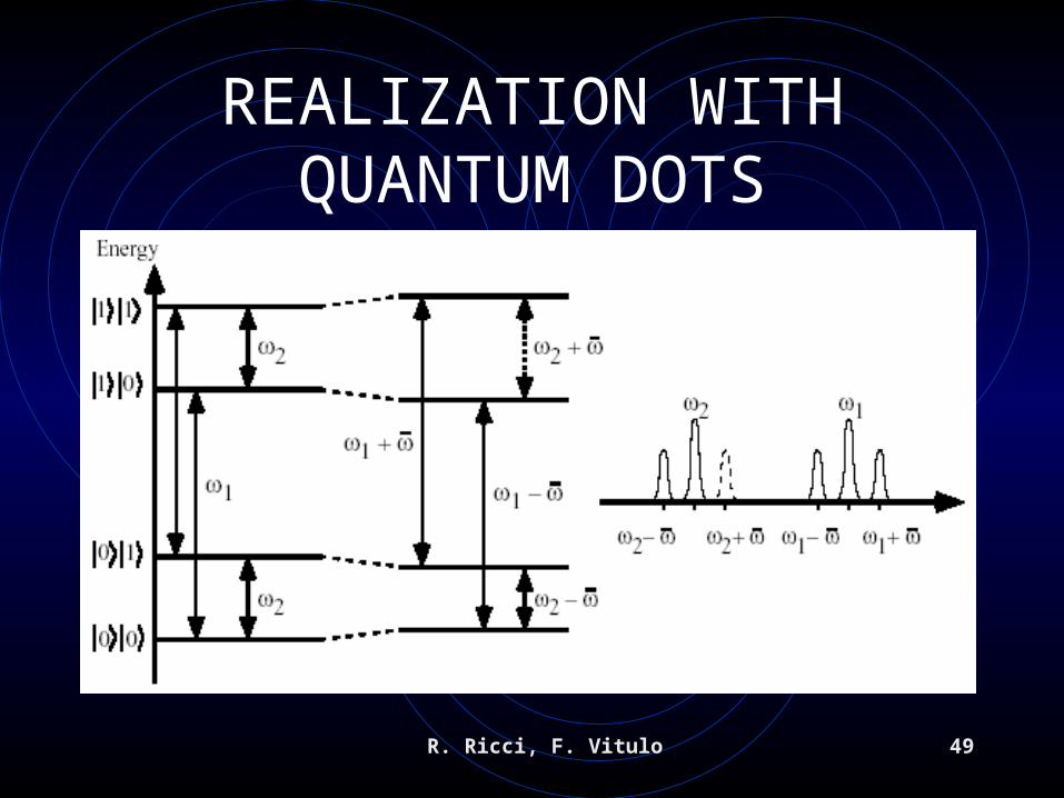
REALIZATION WITH QUANTUM DOTS
• Due to these interactions, the resonant frequency for transitions depends on the neighboring dot’s state.
• First (second) dot’s resonant frequency becomes ( ± ) if second (first) dot is in state |0 or |1, respectively (see picture on next slide).
R. Ricci, F. Vitulo 49
REALIZATION WITH QUANTUM DOTS

R. Ricci, F. Vitulo 50
REALIZATION WITH QUANTUM DOTS
• Thus, a light -pulse at frequency + causes the transitions |0 |1 in the second dot if and only if the first is in state |1.
• In this way, a two quantum dots system can simulate the behavior of a control-NOT quantum gate.

R. Ricci, F. Vitulo 51
ISSUES OF THIS APPROACH
• Decoherence time must be greater than time scale of the optical interaction.
• It is estimated as about 10-6, but impurities and thermal vibration can reduce it to about 10-9 or worse.
• Optical interaction time scale is about 10-9.
R. Ricci, F. Vitulo 52
ISSUES OF THIS APPROACH
• Length of -pulse must be greater than the inverse of dipole-dipole interaction coupling constant.
• In this case: 1012 Hz.
• This model is more difficult to implement than the one based on Ramsey atomic interferometry.

R. Ricci, F. Vitulo 53
ADVANTAGES OF THIS APPROACH
• Effects of decoherence can be reduced with a more precise fabrication technology and by cooling the crystal.
• This approach allows an easy integration of quantum dots into complex quantum circuits, as required for quantum information processing.
R. Ricci, F. Vitulo 54
CONCLUSION: QUANTUM COMPUTING
• Quantum computing is a good challenge for physicist and engineers for the coming years.
• In fact, quantum computers can solve exponentially complex problems in polynomial time.
• So, they give an answer in few seconds to problems that today require lots of years of computation.

R. Ricci, F. Vitulo 55
CONCLUSION: QUANTUM COMPUTING
• The works we presented here are not about the realization of a quantum computer, but they can be considered a big part of it.
• Recently, IBM researchers built a 7-qubit quantum computer which factorized the number 15 in its prime factors 3 and 5.
• Despite its simplicity, it is the most complex quantum calculation ever carried out.
R. Ricci, F. Vitulo 56
REFERENCES
• [1] I. M. Tsai and S. Y. Kuo, “Digital Switcing in the Quantum Domain”, IEEE Trans. on Nanotechnology, vol. 1, no. 3, pp. 154-164, Sep. 2002
• [2] C. P. Williams and S. H. Clearwater, “Explorations in Quantum Computing”, Springer-Verlag
R. Ricci, F. Vitulo 57
REFERENCES
• [3] A. Barenco, D. Deutsch, A. Ekert and R. Jozsa, “Conditional Quantum Dynamics and Logic Gates”, Physical Review Letters, vol. 74, pp. 4083-4086, May 1995
Top Related