


![[Click here are type Paper Title] - Université Laval · Web viewOptical methods, based on holographic interferometry, have been widely applied as diagnostic tools in the conservation](https://static.fdocuments.us/doc/165x107/5ece017757b2e565dd3c1d4c/click-here-are-type-paper-title-universit-laval-web-view-optical-methods.jpg)


Languages
Pages
Legal


HAL Id: hal-01570134https://hal.archives-ouvertes.fr/hal-01570134
Submitted on 28 Jul 2017
HAL is a multi-disciplinary open accessarchive for the deposit and dissemination of sci-entific research documents, whether they are pub-lished or not. The documents may come fromteaching and research institutions in France orabroad, or from public or private research centers.
L’archive ouverte pluridisciplinaire HAL, estdestinée au dépôt et à la diffusion de documentsscientifiques de niveau recherche, publiés ou non,émanant des établissements d’enseignement et derecherche français ou étrangers, des laboratoirespublics ou privés.
Digital holographic interferometry for analyzing highdensity gradients in Fluid Mechanics
Jean-Michel Desse, François Olchewsky
To cite this version:Jean-Michel Desse, François Olchewsky. Digital holographic interferometry for analyzing high densitygradients in Fluid Mechanics. Holographic Materials and Optical Systems, 2017, 978-953-51-3038-3.�10.5772/66111�. �hal-01570134�
Digital holographic interferometry for
analyzing high density gradients in Fluid
Mechanics
Jean-Michel DESSE, François OLCHEWSKY
ONERA, The French Aerospace Lab, 5, Boulevard Paul Painlevé, BP 21261, 59014 LILLE
Cedex, France
Abstract: Digital holographic interferometry has been developed by ONERA for analysing
high refractive index variations encountered in fluids mechanics. Firstly, the authors present
the analysis of a small supersonic jet using three different optical techniques based on digital
Michelson holography, digital holography using Wollaston prisms and digital holography
without reference wave. A comparison of the three methods is given. Then, two different
interferometers are described for analysing high density gradients encountered in high
subsonic and transonic flows. The time evolution of the gas density field around a circular
cylinder is given at Mach 0.7. Finally, a digital holographic method is presented to visualize
and measure the refractive index variations occurring inside a transparent and strongly
refracting object. For this case, a comparison with digital and image holographic
interferometry using transmission and reflection holograms is provided.
Keywords: Digital Holography, Holographic Interferometry, Real-time holography, Phase
measurement.
1. Introduction
In-line and off-axis digital holographic interferometry is now became an optical metrological
tool more and more used in the domain of fluid Mechanics [1]. For instance, it is widely
developed in macro or microscopy for measuring in the flow the particles location or size
[2, 3] or for measuring the temperature or the thermal exchanges in the flames [4, 5]. Others
In-doc controlsIn-doc controlsIn-doc controlsIn-doc controls
authors have developed digital color holographic interferometry by using as luminous
source three different wavelengths (one red, one green and one blue). Qualitative results
have been obtained for visualizing convective flows induced by the thermal dissipation in a
tank filled with oil [6]. Quantitatively, the feasibility of three-wavelength digital holographic
interferometry has been demonstrated for analyzing the variations in the refractive index
induced by a candle flame [7] and the technique has been applied in wind tunnel on two-
dimensional unsteady flows where the time evolution of the gas density field has been
determined on the subsonic near wake flow downstream a circular cylinder [8]. But, when
the flow regime reaches the transonic or supersonic domain, problems appear because
refractive index gradients become very strong and a shadow effect generated by the shock
waves, for instance, superimposes to the micro fringes of interferences. Phase shifts appear
and limit the interferograms analysis. In order to solve these different problems, the authors
propose to study three different cases of flows presenting high density gradients using
specific optical techniques based on digital holography. The first one concerns a small
supersonic jet analyzed by Michelson color digital interferometry, color holographic
interferometry using Wollaston prisms and monochromatic digital holography without
reference wave. The second case is to compare Michelson and Mach-Zehnder
interferometers for analyzing the unsteady wake flow around a circular cylinder at
transonic Mach number. And finally, digital and image holographic methods are presented
to visualize and measure the refractive index variations occurring inside a transparent and
strongly refracting object. For the case of image holographic interferometry, a comparison
with transmission and reflection holograms is provided.
2. Fundamental
Digital holography has been widely developed for analysing diffusive objects since the
digitally reconstructing of the optical wavefront was shown by Goodman and Lawrence [9].
But, in fluid mechanics, the objects under analysis are very often transparent because it is
the field of refractive index of the flow which is measured. There are two ways to measure
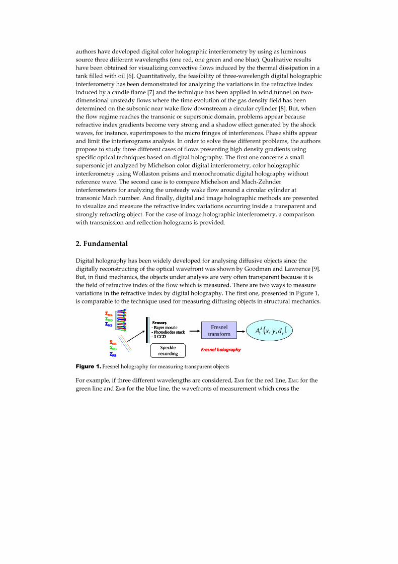
variations in the refractive index by digital holography. The first one, presented in Figure 1,
is comparable to the technique used for measuring diffusing objects in structural mechanics.
Figure 1. Fresnel holography for measuring transparent objects
For example, if three different wavelengths are considered, ΣMR for the red line, ΣMG for the
green line and ΣMB for the blue line, the wavefronts of measurement which cross the
Fresneltransform
Speckle
recordingFresnel holography
ΣΣΣΣMRΣΣΣΣMGΣΣΣΣMB
ΣΣΣΣRRΣΣΣΣRG
ΣΣΣΣRB
ΣΣΣΣMRΣΣΣΣMGΣΣΣΣMB
ΣΣΣΣRRΣΣΣΣRG
ΣΣΣΣRB
:- Bayer mosaic - Photodiodes stack- 3 CCD
Sensors---
( )rr dyxA ,,λFresneltransform
Speckle
recordingFresnel holography
ΣΣΣΣMRΣΣΣΣMGΣΣΣΣMB
ΣΣΣΣRRΣΣΣΣRG
ΣΣΣΣRB
ΣΣΣΣMRΣΣΣΣMGΣΣΣΣMB
ΣΣΣΣRRΣΣΣΣRG
ΣΣΣΣRB
:- Bayer mosaic - Photodiodes stack- 3 CCD
Sensors---
:- Bayer mosaic - Photodiodes stack- 3 CCD
Sensors---
( )rr dyxA ,,λ

transparent object in the test section can be sent on a ground plate and each point of the
plate diffracts and interferes on the sensor with the three reference waves, ΣRR, ΣRG and ΣRB.
In this case, the sensor can be a Bayer mosaic, a stack of photodiodes or a 3CDD. The
recorded image is a speckle image which can be processed using Fresnel transform and the
diffracted field �����, �, �� diffracted at the distance �� and at the coordinates ��, � of the
observation plane is given by the propagation of the three object waves to the recording
plane. The second technique is shown in Figure 2. The three wavelengths ΣMR, ΣMG and ΣMB
interfere directly onto the sensor with the three reference waves, ΣRR, ΣRG and ΣRB. As the
three measurements waves are smooth waves, the interferences with the three reference
waves on the sensor produce three gratings of interference micro-fringes which can be used
as spatial carrier frequencies, one for each wavelength. By using direct and inverse 2D Fast
Fourier Transform (FFT), the amplitude and the phase of the analysed field is obtained.
Figure 2. Fourier holography for measuring transparent objects
All details and basic fundamentals of these two techniques can be found in Picart [10].
3. Digital holography for analysing supersonic jet
In this part, the supersonic flow of a small vertical jet has been analysed using three
different techniques based on digital holography. The first one is based on Michelson digital
holographic interferometer using three wavelengths as luminous source [8], the second one
uses the same source (three wavelengths) and Wollaston prisms to separate the references
waves and the measurement waves [11] and the last one is a little bit particular because a
specific diffraction grating is manufactured to obtain several different diffractions of
measurement waves and to avoid having the reference wave [12].
3.1. Michelson holographic interferometry
The optical setup presented in Figure 3 is very simple and looks like to a conventional
Michelson interferometer in which a beam splitter cube (7) is inserted between the spatial
filter (6) and the aerodynamic phenomenon under analysis (11). The light source consists of
three Diode-Pumped Solid-State lasers, one red (R), one green (G) and one blue (B), emitting
at 660 nm respectively 532 nm and 457 nm. A half wave plate (1) is used to rotate by 90 ° the
polarization of the blue line (S to P) and a flat mirror (2) and two dichroic plates (3) allow to
Fourier transform
Micro-fringes recording
ΣΣΣΣMRΣΣΣΣMGΣΣΣΣMB
ΣΣΣΣRRΣΣΣΣRGΣΣΣΣRB
ΣΣΣΣMRΣΣΣΣMGΣΣΣΣMB
ΣΣΣΣRRΣΣΣΣRGΣΣΣΣRB
:- Bayer mosaic - Photodiodes stack- 3 CCD
Sensors--- ( )yxAr ,λ
Fourier holography
Fourier transform
Micro-fringes recording
ΣΣΣΣMRΣΣΣΣMGΣΣΣΣMB
ΣΣΣΣRRΣΣΣΣRGΣΣΣΣRB
ΣΣΣΣMRΣΣΣΣMGΣΣΣΣMB
ΣΣΣΣRRΣΣΣΣRGΣΣΣΣRB
:- Bayer mosaic - Photodiodes stack- 3 CCD
Sensors---
:- Bayer mosaic - Photodiodes stack- 3 CCD
Sensors--- ( )yxAr ,λ
Fourier holography

superimpose the three wave lengths. An acousto-optical cell (4) deflects the parasitic
wavelengths in a mask (5) and diffracts the three wavelengths RGB using three
characteristic frequencies injected into the crystal. The spatial filter (6), composed with
microscope objective (x60) and a small hole of 25 µm, is placed at the focal length of the
achromatic lens (9) in order to illuminate the phenomenon with a parallel beam. On-going,
50% of the light is returned towards the concave mirror (8) to form the three reference
beams and 50% of the light passes through the test section (10) to form the measuring
waves. The flat mirror (12) placed behind the test section (11) returns the beams in the beam
splitter cube (7). 25% of the light focused on the diaphragm which is placed in front of the
achromatic lens (13). It is the same for the 25% of the reference beam which are focused on
the same diaphragm by the concave mirror (8).
Figure 3. Michelson digital holographic interferometer
Michelson digital holographic interferometer has been implemented around the ONERA
wind tunnel and two optical tables isolate the optical setup from external vibrations. Figure
4 shows the generation of micro-fringes used as spatial carrier frequencies.
Figure 4. Generation and micro-fringes formation by the transparent object
When the focal points of the reference and object waves are superimposed in the diaphragm
which is placed in front of the lens (13), see Figure 3, a uniform background colour is

observed on the screen for each color. The combination of three background color (R, G and
B) produces a white color on 3CCD camera. If the focusing point of the three reference
waves is moved in the plane of the diaphragm, straight interference fringes are introduced
into the field of visualization. This is achieved very simply by rotating the concave mirror
(8). Without flow, these micro fringes are recorded on the 3CCD to calculate the three
reference phase maps. Then the wind tunnel is started and the three object waves are
distorted by the aerodynamic phenomenon. Micro-fringes interferences are again recorded
to enable calculation of the phase maps related to the object. For maps of phase difference,
the reference phase is subtracted from the phase object.This optical technique was tested for
analysing the supersonic flow of a small vertical jet, 5.56 mm in inner diameter at different
pressures of injection. The location of the vertical jet in the middle of the test section is
shown in Figure 3. The exposure time (10 ms) is given by the acousto-optical cell noted (4) in
Figure 3. The fringes space introduced in the field is much narrowed, about four or five
pixels between two successive fringes, in order to generate three high spatial carrier
frequencies. With this configuration, the sensitivity is increased. Each interferogram is
processed with 2D fast Fourier transform and Figure 6 shows the spectra computed for the
reference and measurement and each color plane. One can see that the spatial generated
frequencies are respectively equal to 40.5, 30.9 and 28.4 lines per millimetre for the blue,
green and red lines. Then, a filtering window is selected to cover the useful signal of the
+1order localised in the spectrum and an inverse 2D FFT is applied to reconstruct the
amplitude and the phase of the signal.
Figure 5. 2D spectra computed from the reference and the measurement interferograms
First, the phase maps are calculated from the three reference and three measurement spectra
so that the modulo 2π phase difference maps shown in Figure 6. One can see that the
structures of shocks and decompression appear in the jet. As the difference phase maps are
computed modulo 2π, a phase unwrapping has to be conducted and the results given the
unwrapped phase maps are also presented in Figure 6. At a pressure of 3 bars, we can note
that the phase is varying of 12 radians.

Figure 6. Maps of RGB phase difference (modulo 2π and unwrapped) – P = 3 bars
Finally, the maps of light intensity and optical thickness are calculated from the phase
difference maps. They are presented in Figure 7 for pressures ranging from 2 to 5 bars.
Concerning the maps of the luminous intensity, they are corresponding to figures which
will be obtain if a technique of image holographic interferometry using panchromatic plates
have been used. Knowing the wavelength and the phase, the maps of optical thickness can
be deduced. They are also presented in Figure 7 from 2 to 5 bars. At 2 bars and in the middle
of the compression structures, the optical thickness varies up to 0.2 µm and at 5 bars, it
varies up to 1µm.
Figure 7. Evolution of the luminous intensity and the optical thickness with the pressure

3.2. Three-wavelength holographic interferometry using Wollaston prisms
This part proposes an optical setup based on digital holographic interferometry using two
widely shifting Wollaston prisms and a single crossing of the phenomenon. Each Wollaston
prism is located at the focal point of “Z” astigmatic optical setup. The second Wollaston is
located in the front of the camera and between the two sagittal and transverse focal lines so
that a rotation around the optical axis generates interference micro fringes which are used as
spatial carrier frequency.
3.2.1. Definition of Wollaston prism characteristics
Differential interferometry using Wollaston prism visualizes the light deviation of refractive
index in a direction perpendicular to the direction of the interference fringes. Indeed, in the
case of quartz prism having a very weak pasting angle, the gradient of the refractive index is
measured because the birefringence angle is very weak and the distance between the two
interfering beams is of the order of a few tenths of a millimetre or a few millimetres in the
test section. Data integration is necessary to obtain the absolute refractive index. To avoid
this integration, it was decided to manufacture two Wollaston prisms having a very high
birefringence angle so that the distance between the two interfering beams is greater than
the dimension of the measuring field (jet size). The interference measurement will be made
between a beam which does not pass through the phenomenon (reference beam) and one
which crosses the phenomenon under study. If �� � is the crystal birefringence and �
the pasting angle of prisms, the birefringence angle � can be expressed using the following
equation:
� � ��� � 2�� � tan�� (1)
If a very high birefringence angle is sought, the pasting angle and the crystal birefringence
have to be as high as possible. To remember, the Δ birefringence values for quartz and
calcite are respectively equal to -0.172 and +0.009. It can be seen that calcite birefringence is
basically twenty times greater than quartz birefringence.
If � is the radius curvature of the spherical mirror used in the optical setup, the shift ��
between the two interfering beams can be written as:
�� � �� � 2��� � tan�� (2)
Thus, for a spherical mirror 400 mm in diameter and 4 meters in the radius curvature, ��
has to be near to 200 mm. By choosing calcite crystal, the pasting angle can be found from
the following relationship:
� � arctan � ��� !"# � arctan � $.�
&�$.'(�# � 8.27° (3)
Calcite Wollaston prisms having 8° pasting angle have been manufactured.

3.2.2. Optical setup with single crossing of the test section
The principle of Z optical setup using Wollaston prisms is given in Figure 8. The luminous
light source is also constituted by three different DPSS lasers (red, green and blue) and it
uses two spherical mirrors, 250 mm in diameter and 2.5 m in radius of curvature.
Figure 8. Digital holographic interferometer using very large Wollaston prisms in “Z” setup
This arrangement has the particularity of introducing the astigmatism because all optical
pieces are not exactly on the optical axis of spherical mirrors. The first prism is located at the
focal length of the first spherical mirror so that the two optical rays which are returned on
the second spherical mirror are constituted by parallel light beams. The second spherical
mirror refocuses the light beam into the second Wollaston prism which is mounted
“tumble” with the first one. An analyser is then placed behind the second prism in order to
visualize the interference fringes in color. A field lens placed in front of the camera forms
the image of the object under analysis on the 3CCD sensor. Here, we can use the advantage
of astigmatic setup because the focusing point in the front of the camera is not unique.
Figure 9 shows that the optical beams are focused on the two focal images successively
separated by a few millimetres. The first one encountered is the result of the focusing beam
in the horizontal plane, it is the tangential image and the second one is called the sagittal
image, it is the result of the focusing beams in the vertical plane.
Figure 9. Astigmatism represented by sectional views and Wollaston prism in the front of the camera
Microscopeobjective
Object
Polarizer
Large fieldWollaston prism
Spherical mirror
Hamamatsu3CDD
Condenser
Analyser
Spherical mirror
Large fieldWollaston prism
λ1 = 457 nm
λ2 = 532 nm
λ3 = 660 nm
Microscopeobjective
Object
Polarizer
Large fieldWollaston prism
Spherical mirror
Hamamatsu3CDD
Condenser
Analyser
Spherical mirror
Large fieldWollaston prism
λ1 = 457 nm
λ2 = 532 nm
λ3 = 660 nm
dsds
Objectpoint
Optical axis
Tangential image
Sagittal image
Optical system
dsds
Objectpoint
Optical axis
Tangential image
Sagittal image
Optical system
dsds
Objectpoint
Optical axis
Tangential image
Sagittal image
Optical system
dsds
Objectpoint
Optical axis
Tangential image
Sagittal image
Optical system

In Figure 10, on the reception side, when the second Wollaston prism is successively moved
along the optical axis towards the sagittal image (SI), the interferences fringes which were
horizontal and much narrowed, spread. When the Wollaston prism is moved from the
sagittal image (SI) to the tangential image (TI), the interference fringes spread again, but
they rotate by 90° to give a quasi-uniform vertical background color, at half distance
between the tangential and sagittal images. Then, they continue to rotate by 90° up to the
sagittal image and they narrow to become horizontal. Above the sagittal image, interference
fringes stay horizontal and narrow more and more. It follows that the spatial carrier
frequency can be adjusted by the axial displacement of the prism for its amplitude and by
rotating the prism for its orientation. In these experiments, the Wollaston prism is located at
half distance between the tangential and sagittal images, because it generates interference
fringes in the same direction as the direction of the two interfering beams (vertical shift and
vertical fringes). This feature was described by Gontier [13]. To increase the number of
fringes in the visualized field, the Wollaston prism has to be turned on itself in the plane
perpendicular to the optical axis. Two positions are shown in Figure 10 (20° and 45°) where
one can see that the maximum number of fringes is obtained for a rotation of 45°.
Figure 10. Evolution of interference fringes when the second Wollaston is moved from the sagittal
image to the tangential image
3.2.3. Results obtained
Firstly, Figure 11 shows the interferograms for the reference and the measurement with an
enlarged view near the injection. For a pressure of 4 bars, for instance, one can see the
horizontal interference fringes disturbed by the flow. The interferograms of Figure 10 also
show that the field is reduced on the right and left sides: this is the result of the rotation of
the Wollaston prism at return which has a limited size (15 mm² square). The polarization
fields which were completely separated on the way interfere with each other as the prism
placed in front of the camera is rotated. It is also noteworthy that the polarizer is rotated
exactly the same amount as the Wollaston prism. The tightening of the fringes is maximal
when the prism is rotated by 45°.

Figure 11. Interference micro-fringes recorded for the reference and the measurement – P = 4 bars
Then, 2D Fast Fourier Transform is applied to filter the zero and -1 orders on the three
channels for the reference and the measurement interferograms. In Figure 12, one see that
the window filtering size can be taken different on the three channels and that the reduced
frequencies are equal to 0,12, 0,10 et 0,9 mm-1 for the blue, green and red channels that
corresponds to resolution of 18,6 lines/mm, 15,5 lines/mm and 13,9 lines/mm. The spatial
resolution is lower than in the technique of Michelson interferometry.
Figure 12. 2D spectra computed on the three channels for the reference interferogram - P= 4 bars
Figure 13 shows the spectrum of the measurement for P = 3 bars, the modulo 2π phase map,
the superimposition of the three red, green and blue luminous intensities deduced from the
phase difference maps and also the optical thickness map computed from the phase
difference map. Theses maps are concerning the red channel. Moreover, a deconvolution of
the optical thickness maps based on the assumption that the jet is axisymmetric has been
applied. Thus, it is possible to obtain the radial distribution of the refractive index and the
density in the jet according to the relation Gladstone-Dale. This method is widely described
in Rodriguez [14]. In the treatment process, the optical thickness of maps calculated for each
jet pressure is split into two parts, on either side of the axis of symmetry of the jet. If the
results found by both sides of the jet are identical to the symmetry axis, the assumption of
the axial jet symmetry is verified and the results can be considered correct. In Figure 12, the
radial gas density is presented at 3 bars and the density values found on the axis are very
close, the analysis being done on the right or on the left.

Figure 13. Analysis of the case for red channel P = 3 bars (from spectrum to gas density)
3.3. Digital holography without reference wave
Digital holography without reference wave allows quantitative phase imaging by using a
high resolution holographic grating for generating a four-wave shearing interferogram. The
high-resolution holographic grating is designed in a “kite” configuration so as to avoid
parasitic mixing of diffraction orders. The selection of six diffraction orders in the Fourier
spectrum of the interferogram allows reconstructing phase gradients along specific
directions. The spectral analysis yields the useful parameters of the reconstruction process.
The derivative axes are exactly determined whatever the experimental configurations of the
holographic grating. The integration of the derivative yields the phase and the optical
thickness [12].
3.3.1. Base of digital holography without reference
Figure 14 shows the principle of the hologram recording of pure phase modulation where
an incident plane crosses the phenomenon under analysis. This wave, disturbed by the
phenomenon, is simultaneously diffracted in several directions by a diffraction grating
operating in reflection. The different images diffracted by the grating interfere with each
other at a distance of the diffraction plane.
Figure 14. Principle of self-referenced digital holography by reflection
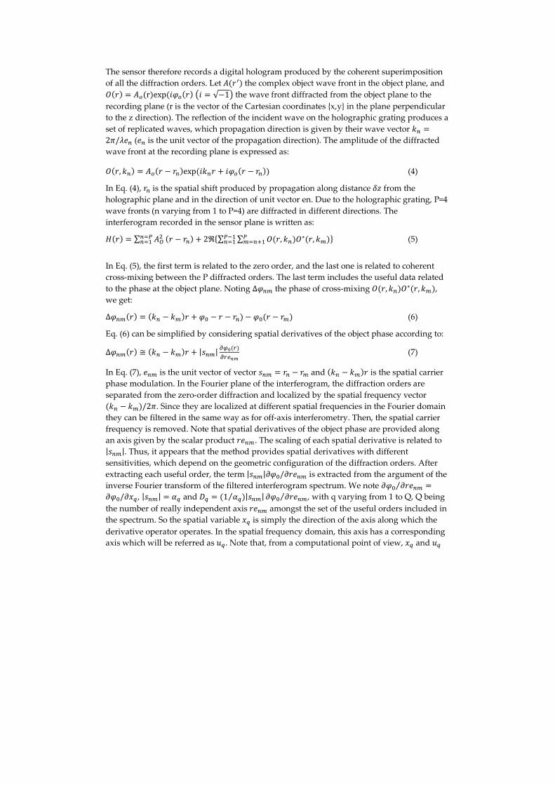
The sensor therefore records a digital hologram produced by the coherent superimposition
of all the diffraction orders. Let ��,- the complex object wave front in the object plane, and
.�, � � �rexp�23 �, 42 � √�17 the wave front diffracted from the object plane to the
recording plane (r is the vector of the Cartesian coordinates {x,y} in the plane perpendicular
to the z direction). The reflection of the incident wave on the holographic grating produces a
set of replicated waves, which propagation direction is given by their wave vector 8" �29/�;" (;" is the unit vector of the propagation direction). The amplitude of the diffracted
wave front at the recording plane is expressed as:
.�,, 8" � � �, � ,"exp�28", < 23 �, � ," (4)
In Eq. (4), ," is the spatial shift produced by propagation along distance => from the
holographic plane and in the direction of unit vector en. Due to the holographic grating, P=4
wave fronts (n varying from 1 to P=4) are diffracted in different directions. The
interferogram recorded in the sensor plane is written as:
?�, � ∑ �A�"BC"B' �, � ," < 2DE∑ ∑ .�,, 8"C
FB"G'CH'"B' .∗�,, 8FJ (5)
In Eq. (5), the first term is related to the zero order, and the last one is related to coherent
cross-mixing between the P diffracted orders. The last term includes the useful data related
to the phase at the object plane. Noting Δ3"F the phase of cross-mixing .�,, 8".∗�,, 8F, we get:
Δ3"F�, � �8" � 8F, < 3$ � , � ," � 3$�, � ,F (6)
Eq. (6) can be simplified by considering spatial derivatives of the object phase according to:
Δ3"F�, ≅ �8" � 8F, < |M"F| NOP��N��QR (7)
In Eq. (7), ;"F is the unit vector of vector M"F � ," � ,F and �8" � 8F, is the spatial carrier
phase modulation. In the Fourier plane of the interferogram, the diffraction orders are
separated from the zero-order diffraction and localized by the spatial frequency vector
�8" � 8F/29. Since they are localized at different spatial frequencies in the Fourier domain
they can be filtered in the same way as for off-axis interferometry. Then, the spatial carrier
frequency is removed. Note that spatial derivatives of the object phase are provided along
an axis given by the scalar product ,;"F. The scaling of each spatial derivative is related to
|M"F|. Thus, it appears that the method provides spatial derivatives with different
sensitivities, which depend on the geometric configuration of the diffraction orders. After
extracting each useful order, the term |M"F|S3$/S,;"F is extracted from the argument of the
inverse Fourier transform of the filtered interferogram spectrum. We note S3$ S,;"F⁄ �S3$/S�U , |M"F| � �U and VU � �1 �U|M"F|⁄ S3$ S,;"F⁄ , with q varying from 1 to Q, Q being
the number of really independent axis ,;"F amongst the set of the useful orders included in
the spectrum. So the spatial variable �U is simply the direction of the axis along which the
derivative operator operates. In the spatial frequency domain, this axis has a corresponding
axis which will be referred as WU. Note that, from a computational point of view, �U and WU

are 2D vectors. In case that the VU exceed 2π, phase jumps occur and phase unwrapping is
required. The scaling coefficient �U depends on the distance => and on the couple of
involved wave vectors �8", 8F. Then, the spatial integration of terms VU has to be carried
out to get the quantity X. The wave-front reconstruction problem has already been
discussed by many authors and the methods are based on least-squares estimations or
modal estimations. Note that in these works the wave front differences are defined at each
point according to the sensor sampling geometry. In the modal approach, the wave front
and its differences are expanded in a set of functions and the optimal expansion coefficients
are determined (for example, using Zernike and Legendre polynomials). Here, the
numerical method is based on the weighted least square criterion and according to
references [15, 16], quantity X can be recovered.
3.3.2. Design of diffraction grating
First, a holographic grating is recorded with the optical setup shown in Figure 15. The
holographic plates are single-layer silver-halide holographic plates from Gentet
(http://www.ultimate-holography.com/). The spatial resolution reaches 7.000 lines per mm.
Figure 15. Optical setup defined for recording of reflection holographic grating
A first beam splitter cube (80/20) forms a reference beam (blue beam) with 20% of the
incident light and 80% of the light is used to form the four object beams. Plane waves are
obtained with two lenses and two spatial filters. Object waves are generated by three beam
splitter cubes (50/50) so that the luminous intensities of each beam (reference and object) are
all equal to 20% of the initial laser power. After several reflections on flat mirrors (MP), four
small mirrors located around a square (configuration n°1) and around a kite (configuration
n°2) returns each object beams towards the holographic plate. As the reference wave and the
four object waves are incoming on each side of the hologram, the hologram is recorded by
Hologram
BS
50/50
BS
50/50
BS
50/50
BS
80/20
Spatial
filter
Acousto-
optic cellSpatial
filter
Reference wave
Flat mirror (MP)
MP
MP
MP
MP
MP
MP
MP
l= 532 nm
20
80
40
40
20
20
20 20
12 cm
Reference
wave
12
cm
Configuration°1
18 cm
Reference
wave
18
cm
Configuration°2
Hologram
BS
50/50
BS
50/50
BS
50/50
BS
80/20
Spatial
filter
Acousto-
optic cellSpatial
filter
Reference wave
Flat mirror (MP)
MP
MP
MP
MP
MP
MP
MP
l= 532 nm
20
80
40
40
20
20
20 20
12 cm
Reference
wave
12
cm
Configuration°1
18 cm
Reference
wave
18
cm
Configuration°2

reflection and the angles θ formed by the reference and the object waves are equal to 27mrad
for configuration n°1. After four sequential exposures, one for each object wave, the
holographic plate is developed and bleached. Then, the grating is inserted in the optical
setup which is used for analysing the small supersonic jet from a nozzle. Figure 16 shows
the optical setup with a single crossing of the phenomenon at the distance δz between the
sensor and the image of the high-resolution holographic grating (HRHG).
Figure 16. Digital holographic interferometer without reference
An interferogram without flow and an interferogram with flow are directly recorded on the
sensor (2000x1500 pixels, 3,65mm square), then analysed in delayed time by 2D fast Fourier
transform in order to localize the different interference orders. For configuration n°1, Figure
17 shows the location of four mirrors used at the recording (square). Order 1 results of
interaction of the beams incoming from M1 and M2 mirrors and the order 1’ between M3
and M4. Similarly, order 2 is generated by the interference between the waves incoming
from M1 and M3 mirrors and order 2’ those issuing from M2 and M4. Order 3 is only
produced by the interference between M1 and M4 and order 4 between M2 and M3. For
configuration n°1, order 1 or 2 has been enlarged in order to show that order 1 and 1’ or 2
and 2’ are not quite superimposed.
Figure 17. Position of four mirrors (square and kite) at the recording, localization of different
diffraction orders in 2DFFT plane and zoom of +1 order.
In fact, one obtains two spectral signatures slightly shifted. It is not possible to separate
them by filtering and to reconstruct the phase derivative map induced by only order 1. For
this reason, the four mirrors have been set at the four tops of a kite configuration (n°2). The
problem encountered with configuration n°1 doesn’t exist and 2DFFT shows that it is very

easy to localize all the different diffraction orders (on right in Figure 17). There is no spectral
overlap and all orders useful for the reconstruction are well separated. Each order of
interference is then selected successively and separately with a circular mask (20mm-1
radius). Then, the phase gradient of reference image is calculated for each order of
interference (Figure 18). Subtracting the reference image to the measurement image gives a
modulo 2π map of phase gradient difference caused by the flow. Then, difference phase
maps have to be unwrapped and results are presented in Figure 18 for the six diffracted
orders and for a value of the generating pressure equal to 5 bars. Finally, knowing the phase
gradient difference in the six directions, a reconstruction of the absolute phase map is
possible. For this processing of integration calculation, one can use one of integration
methods proposed in the literature, for instance that proposed by Frankot and Chellappa
[15]. The modulus of complex amplitude and the optical phase of the diffracted field by the
object can be combined for obtaining the complex wave diffracted in the sensor plane.
Figure 18. Recorded interferogram and gradient phase maps obtained for the six interference orders
3.4. Comparisons with digital holographic interferometry using a reference wave
Figure 19 shows results obtained with digital holographic interferometry without reference
and two others results obtained with digital holographic interferometry using a reference
wave. The comparison is made by taking into account the difference of optical thickness.
Figure 19. Comparison of experimental results obtained for three different interferometric techniques
for a pressure at P=5 bars, (a) Without reference setup, (b) Michelson set-up, (c) Wollaston setup.

The scale level is basically the same for the three results (from 0 up to 1.2 µm) and Figure 19
shows at 5 bars that they are in good agreement because spatial locations of the structures of
compression and expansion waves are similarly positioned in the three measurements.
4. Digital holography for analysing unsteady wake flows
The unsteady wake flows generated in wind tunnel present a large scale of variations in
refractive index from subsonic to supersonic domain. The feasibility of three-wavelength
digital holographic interferometry has been shown on two-dimensional unsteady flows and
the time evolution of the gas density field has been determined on the subsonic near wake
flow downstream a circular cylinder [8]. But, when the flow regime reaches the transonic or
supersonic domain, problems appear because refractive index gradients become very strong
and a shadow effect superimposes to the micro fringes of interferences. Moreover, the
displacement of vortices is very high compared to the exposure time (300 ns given by the
acousto-optical cell, Figure 3) what leads to blurred zones in interferograms and limits the
interferograms analysis (Figure 20).
Figure 20. Highlighting of blurred areas and shadow effect – Mach 0.73
4.1. Michelson holographic interferometry
Firstly, an ORCA Flash 2.8 camera from Hamamatsu with a matrix of 1920x1440 pixels,
3.65 µm² square, has been bought to increase the spatial resolution and, for the temporal
resolution, the continuous laser light source of the interferometer has been replaced by a
Quanta-Ray pulsed laser, Model Lab 170-10Hz from Spectra-Physics. This laser is injected
through a 1064 nm laser diode and outputs a wavelength at 1064 nm having 3 meters in
coherence length (TEM00 mode). Here, the first harmonic is used (532 nm) and delivers
about 400 mJ in 8 nanoseconds. The beam diameter is about 8 to 9 mm. Figure 21 shows how
the laser was installed in Michelson interferometer presented in Figure 3. The output beam
is equipped with two sets “λ/2-polarizing beam splitter cube” to significantly reduce the
laser energy sent to the camera. It is seen in Figure 21 that the beam splitter cube forms the
reference wave which is reflected by the concave mirror on the camera and the
measurement wave which passes through the test section. The second achromatic lens, 70
mm in focal length of 70 mm yields the magnification of the image on the CCD.

Figure 21. Digital Michelson holographic interferometer using a pulsed laser
If L1 is the distance between the beam splitter cube and the concave mirror, and L2 the
distance between the same beam splitter cube and the flat mirror located behind the test
section, the laser coherence length must be greater than twice the difference (L2 - L1) for the
interference fringes may be formed on the CCD. This difference is here of the order of 2.5 m.
Figure 22 shows an interferogram of unsteady wake flow around a circular cylinder at Mach
0.73 with Michelson interferometer, the 2D FFT spectrum with the +1 order used to
reconstruct the map of the modulo 2πphase difference. The interferogram exhibits a good
quality indicating that vortex structures and small shock waves are well frozen. But, in the
modulo 2π phase difference map shown on the right of Figure 22, phase jumps are still
present. They are surrounded by black ellipses on the figure and they will cause phase shifts
during the unwrapping of the modulo 2π phase map. To decrease the sensitivity of the
measurement by a factor of 2, the optical bench has been modified to create a Mach-Zehnder
type bench.
Figure 22. Interferogram analysis at Mach 0.73 – Residual phase shifts
4.2. Mach-Zehnder holographic interferometry
In Mach-Zehnder interferometer shown in Figure 23, the measuring beam crosses only once
the test section and the reference beam passes outside the test section so that the sensitivity
is decreased by a factor 2.
λ2= 532 nmλ = 532 nm
λ/2 λ/2
Polarizing beam splitter cube
Mask
Spatial filter
f 110 mm
f 70 mm
Interference fringes
Orca Flash 2.2 camera
f 800 mm
Cylinder
Flat mirror
Windows
Pulsed laser
λ2= 532 nmλ = 532 nm
λ/2 λ/2
Polarizing beam splitter cube
Mask
Spatial filter
f 110 mm
f 70 mm
Interference fringes
Orca Flash 2.2 camera
f 800 mm
Cylinder
Flat mirror
Windows
Pulsed laser

Figure 23. Digital Mach-Zehnder holographic interferometer using a pulsed laser
In this optical setup, the reference beam is reflected successively by several little flat mirrors.
That produces a polarization rotation of the reference wave which must be corrected by
inserting a λ/2 plate in front of the spatial filter of the reference wave. The contrast of the
interference fringes can thus be optimized on the interferogram. The cylinder is equipped
with an unsteady pressure transducer at a 90° azimuth to the flow axis in order to correlate
the laser pulse with the signal of unsteady pressure. In this manner, one period of the
phenomenon can be sampled by 20° step with several different tests. First, in the enlarged
part of reference and measurement interferograms of Figure 24, one can see the straight
interference micro fringes distorted by the shear layer incoming from the upper of the
cylinder. 2D FFT spectra show that the spatial carrier frequency (vertical fringes) is localized
on horizontal axis (order +1 of hologram). After applying a spatial filter around the first
order and subtracting the reference to the measurement phase map, one obtains the modulo
2π phase difference map where no phase shifts appear.
Figure 24. Interferograms analysis at Mach 0.73
Then, an unwrapping has to be applied to obtain the phase difference map ∆φ and the gas
density field ρ/ρ0 presented in Figure 25 is deduced from the Gladstone-Dale relationship
and Equation (8):
(8)
Camera
Flat mirror
Screen
Interferencefringes
f 800 mm
f 120 mm
f70mmф40mm
λ2= 532 nmλ = 532 nm
λ/2 λ/2
Polarizing beam splitter cube
Mask
Spatial filter
Spatial filter
λ/2
Flat mirror
50
50
f 800 mm
Pulsed laser
Camera
Flat mirror
Screen
Interferencefringes
f 800 mm
f 120 mm
f70mmф40mm
λ2= 532 nmλ = 532 nm
λ/2 λ/2
Polarizing beam splitter cube
Mask
Spatial filter
Spatial filter
λ/2
Flat mirror
50
50
f 800 mm
Pulsed laser

where is the standard gas density computed at 1 atmosphere and 0° C, the stagnation
gas density, λ the wavelength of the interferometer, e the width of the test section and K the
Gladstone-Dale constant: 296.10-6.
The instantaneous interferogram of Figure 25 shows that shock waves emitted by the
vortices of the vortex shading are very well analysed (no phase shift) and the averaged gas
density field exhibits a strong decreasing of the gas density just behind the cylinder up to
90% of . For information, the shadow effect can be easily reduced. If the beam of the
reference arm is blocked (see Figure 23), the Mach-Zehnder interferometer looks like to
shadowgraph optical setup. In these conditions, the sensor can be adjusted along the optical
axis to focus and image the middle of the test section on the sensor. As this condition is
reached, the shadow effect is minimized.
Figure 25. Instantaneous and averaged gas density fields (ρ/ρo) – Mach 0.73
5. Digital holography for visualizing inside strongly refracting
transparent objects
High density gradients can also exist inside strongly refracting objects and the visualization
and the measurement of these phenomena remain an open problem. For example, objects as
a glass ball, a light bulb, a glass container, a glass flask, …, are not opaque but they are
strongly refracting light and measuring inside is not straightforward. It follows that
observing phenomena, such as refractive index variations, convection currents, or thermal
gradients, occurring inside the object requires specific methods. Different experimental
methods are usually used to investigate fluids and to visualize/measure dynamic flows [7, 8,
17]. Nevertheless, these approaches are appropriated when the envelope including the flow
is relatively smooth and transparent (i.e. not strongly refracting). A suitable experimental
method should be able to exhibit the phase changes inside the object without suffering from
any image distortion. The experimental approach described here is based on stochastic
digital holography to investigate flows inside a strongly refracting envelope. It leads to the
measurement of the phase change inside the object, so as to get a quantitative measurement.
Experimental results are provided in the case of the visualization of refractive index
variations inside a light bulb and a comparison with image transmission and reflection
holography is also provided.

5.1. Proposed method
The approach adapted to visualize inside a strongly refracting object is described in Figure
26. The sensor includes N×M=1920×1440 pixels with pitches px=py=3.65µm. The main feature
is that a diffuser is used to illuminate the object to provide a back illumination. The set-up
exhibits some similarity compared to a classical transmission microscope, although, no
microscope objective is used and the illuminating wave is quite a speckled wave. A negative
lens is put in front of the cube to virtually reduce the object imaged by this lens. This leads
to a more compact system compared to the case where the lens is not used. For example, for
an object size of 10-15cm, the distance d0 in Figure 26 has to be greater than 2m. The use of
the negative lens produces a smaller image of the image, which position is close to the
sensor [18, 19]. Thus the distance than has to be used in the algorithm is d’0 (see Figure 25).
The optimization of the off-axis the set-up has to follow the basic rules about the Shannon
conditions [20].
Figure 26. Stochastic digital holographic setup
Particularly, the focal length of the lens has to be judiciously chosen. Especially, the criterion
is the observation angle from the sensor, which has to fulfil this condition:
(9)
where α is the accepted tolerance in the superposition of the useful +1 order and the 0 order.
Here, the diffuser (considered here as a “stochastic screen”) is sized 10cm×20cm and a
superposition tolerance of α=20% is accepted. The evaluation of the focal length and
distance leads to d0=800mm, d’0=100mm and f’=−150mm. Holograms can be reconstructed by
the adjustable magnification method described in [21] or by the discrete Fresnel transform
[18-20]. After reconstruction of the complex amplitude in the virtual object plane, an
amplitude image and a phase image can be calculated. The amplitude image is related to the
image of the object given by the lens, whereas the phase is useful to investigate refractive
index variations, convection currents, or thermal gradients, occurring inside the object. For
this, one has to evaluate the temporal phase difference at different instants. A quantitative
measurement can be obtained after unwrapping the phase differences. Since the refractive
index variations are encoded in the unwrapped phase, the use of the Gladstone-Dale
relation allows determining density variations.

5.2. Proof of principle
The proposed method has been applied to the visualization and analysis of light bulb
during its lighting. This bulb was submitted to a current to produce light and holograms
were recorded at different instants after its lighting. Figure 27 shows the recorded hologram
when the bulb is off (a) and when the bulb is lighting (b). The speckle nature of the
hologram is clearly observed. Figure 27c) shows the amplitude image obtained with the
discrete Fresnel transform. The stochastic screen and the ampoule can be clearly seen so that
the strand of the bulb. Figure 27 d) and e) show respectively the modulo 2π digital fringes
and unwrapped phase differences obtained between two instants (light off and light on).
One can note a very large amplitude variation since the phase values are in the range 10
radians to 50 radians (see the colorbar in Figure 27e)). This measurement includes the
contribution due to the refractive index change in the bulb and also a contribution due to the
dilatation of the envelope and its refractive index variation due to the temperate increase
inside the lamp (≈500°C). The “numerical fringes” observed in Figure 27d) exhibits the
refractive index variations integrated in the glass container.
Figure 27. Quantitative measurement inside the bulb, a)virtual phase extracted from numerical
reconstruction (bulb off), b)bulb lighting, c) image amplitude of the strand, d)modulo 2π phase
computed from (a) and (b), e)unwrapping of (d)
5.3. Comparison with silver-halide plate holographic interferometry
In order to check for the quality of the results obtained with the proposed method, the
results obtained were compared with analogue image-holography [22]. The two possible
setups are described in Figure 28 and can be either transmission or reflection holographic
interferometry. Figure 28a) shows the transmission holography mode and Figure 28b) that
for reflection holography. Note that the set-ups require the use of photographic plates and
that the diffuser is also used to get a stochastic screen to illuminate the object. The process is
as follows: record a transmission or reflection hologram, apply the chemical treatment to the
plate to develop and bleach, dry the plate, put the holographic plate in the set-up anew
(exactly at the same location), at this step the holographic image of the ampoule is
observable, adjust the camera lens to produce a focused image, then record real-time
interferences between the initial bulb and that currently submitted to the current. Note that

only the luminous intensity of interference fringes can be obtained, and not the phase image
as it is the case for the digital holographic approach.
Figure 28. Image transmission holography(a) and image reflection holography (b)
Figure 29 shows a comparison between results obtained with digital holography and those
obtained with image holography. Figure 29a) shows the image obtained with the amplitude
and phase change measured by digital holography, after calculating the intensity
, where is the phase change and A the amplitude image. Figure 29b) shows the
interference fringes obtained with the set-up of Figure 28a) and Figure 29c) shows those
obtained with the set-up of Figure 28b). A very good agreement can be observed.
Furthermore, the image quality given by each method can be appreciated. Image
holography provides the best spatial resolution: the strand of the lamp can be clearly seen in
Figure 29b) and c). However, digital holography is more flexible since no chemical
processing is required and a phase image can be obtained.
Figure 29. Comparison between intensity of fringes, (a) fringes calculated with digital holography, (b)
fringes obtained with transmission holography, (c) fringes obtained with reflection holography
6. Conclusion
This chapter has shown several possibilities of digital holographic interferometry for
analysing high density gradients encountered in transonic and supersonic flows.
Concerning the analysis of a small supersonic jet, a comparison is given between three
different techniques, two techniques use reference waves: Michelson holographic
interferometry and digital holography using Wollaston prisms; The last one uses a specific

diffraction grating to obtain several different diffractions of measurement waves and to
avoid having the reference wave.
For analysing transonic flows in wind tunnel, two types of interferometer have been
developed. The first one is very simple to implement because it is a Michelson
interferometer with double crossing of the test section for increasing the sensitivity and the
second one is a Mach-Zehnder interferometer, more difficult to adjust, with a single crossing
of the test section. These two interferometers are equipped with a pulsed laser and
interferograms obtained have a very good quality and, basically, no phase shift.
Finally, a digital holographic method is proposed to visualize and measure refractive index
variations, convection currents, or thermal gradients, occurring inside transparent but
strongly refracting object. The principle of this technique is provided through the
visualization of refractive index variation inside a lighting ampoule. Comparisons with
image transmission and reflection holographic interferometry demonstrate the high image
and phase quality that can be extracted from the stochastic digital holographic setup.
Currently, digital holographic interferometry is developed by ONERA for studying 3D
flows from multi directional tomographic interferograms recorded in several directions. The
aim is firstly to compare this method with others techniques yielding the gas density field as
differential interferometry, back oriented schlieren (BOS) and color BOS and secondly, to
find the best compromise between the number of sight of view, the computation time and
the results accuracy.
7. Acknowledgments
The authors thank the French National Agency for Research (ANR) for founding this work
under Grant agreement n° ANR-14-ASTR-0005-01.
8. References
[1] Katz J, Sheng J. Applications of holography in fluid mechanics and particle dynamics.
Annu. Rev. Fluid Mech.. 2010;42
[2] Atlan M, Gross M, Desbiolles P, Absil E, Tessier G, Coppey-Moisan M. Heterodyne
holographic microscopy of gold particles. Opt. Letters. 2008;33(5)
[3] Müller J, Kebbel V, Jüptner W. Characterization of spatial particle distributions in a
spray-forming process using digital holography. Meas. Sci. Technol.. 2004;15
[4] Sharma S, Sheoran G, Shakher C. Investigation of temperature and temperature profile
in axi-symmetric flame of butane torch burner using digital holographic
interferometry. Opt. Lasers Eng.. 2012;50
[5] Dolocek R, Psota P, Ledl V, Vit T, Vaclavik J, Kopecky V. General temperature field
measurement by digital holography. App. Opt.. 2013;52(1)

[6] Demoli N, Vukicevic D, Torzynski M. Dynamic digital holographic interferometry
with three wavelengths. Opt. Express. 2003;11(7)
[7] Desse JM, Picart P, Tankam P. Digital three_color holographic interferometry for flow
analysis. Opt. Express. 2008;16(8)
[8] Desse JM, Picart P, Tankam P. Digital three-color holographic interferometry applied
to fluid and structural mechanics. Opt. Lasers Eng.. 2012;50
[9] Goodman JW, Lawrence RW. Digital image formation from electronically detected
holograms. App. Phys. Letters. 1967;11
[10] Picart P, Gross M, Marquet P. Basic Fundamentals of digital holography. In: Picart P.,
editor. New techniques in digital holography. ISTE WILEY; 2015.
[11] Desse JM, Picart P. Quasi-common path three-wavelength holographic interferometr
based on Wollaston prisms. Opt. Lasers Eng.. 2015;68
[12] Desse JM, Picart P, Olchewsky F. Quantitative phase imaging in flows with high
resolution holographic diffraction grating. Opt. Express. 2015;23(18)
[13] Gontier G, Carr P, Henon G. Sur un dispositif d'interféromtrie différentielle
permettant d'orienter arbitrairement les franges par rapport à la direction du décalage
des faisceaux. Compte-rendu à l'Académie des Sciences. 1966;Tome 262
[14] Rodriguez O, Desse JM, Pruvost J. Interaction between a supersonic jet and a coaxial
supersonic flow. Aerospace Science and Technology. 1997;11(6)
[15] Frankot RT, Chellappa. A method for enforcing integrability in shape from shading
algorithms. In: Horn BKP and Brooks MJ, editors. Shape and shading. 1989.
[16] Velghe S, Primot J, Guérineau N, Cohen M, Wattelier B . Wave-front reconstruction
from multidirectional phase derivatives generated by multilateral shearing
interferometers. Opt. Lett.. 2005;30(3)
[17] Kakue T, yonesaka R, Tahara T, Awatsuji Y, Nishio K, Ura S, Kubota T, Matoba O.
High-speed phase imaging by parallel phase-shifting digital holography. Opt. Lett..
2011;36(21)
[18] Schnars U, Kreis TM, Jüptner WO. Digital recording and numerical reconstruction of
holograms: reduction of the spatial frequency spectrum. Opt. Eng.. 1996;35
[19] Mundt J, Kreis T. Digital holographic recording and reconstruction of large scale
objects for metrology and display. Opt. Eng.. 2010;49
[20] Picart P, Leval J. General theoretical formulation of image formation in digital Fresnel
holography. JOSA A. 2008;25(7)
[21] I JC, Tankam P, Pen Z, Picart P. Digital holographic reconstruction of large objects
using a convolution approach and adjustable magnification. Opt. Lett.. 2009;34(5)
[22] Desse JM, Tribillon JL. Real-time three-color reflection holographic interferometer.
App. Opt.. 2009;48(36)
Top Related