


Languages
Pages
Legal


Developing a "Severe Test" of Species Distribution Modelling
for Conservation Planning
Submitted by
Paul Andrew Zorn
A THESIS SUBMITTED IN PARTIAL FULFILMENT OF
THE REQUIREMENTS FOR THE DEGREE OF
DOCTOR OF PHILOSOPHY IN THE DEPARTMENT OF BIOLOGY
Supervisors: Kathym Lindsay, Ph.D. and Lenore Fahrig, Ph.D.
CARLETON UNIVERSITY
May 2012
©Paul Andrew Zorn, 2012

Library and Archives Canada
Published Heritage Branch
Bibliotheque et Archives Canada
Direction du Patrimoine de I'edition
395 Wellington Street Ottawa ON K1A0N4 Canada
395, rue Wellington Ottawa ON K1A 0N4 Canada
Your file Votre reference
ISBN: 978-0-494-89207-7
Our file Notre reference
ISBN: 978-0-494-89207-7
NOTICE:
The author has granted a nonexclusive license allowing Library and Archives Canada to reproduce, publish, archive, preserve, conserve, communicate to the public by telecommunication or on the Internet, loan, distrbute and sell theses worldwide, for commercial or noncommercial purposes, in microform, paper, electronic and/or any other formats.
AVIS:
L'auteur a accorde une licence non exclusive permettant a la Bibliotheque et Archives Canada de reproduire, publier, archiver, sauvegarder, conserver, transmettre au public par telecommunication ou par I'lnternet, preter, distribuer et vendre des theses partout dans le monde, a des fins commerciales ou autres, sur support microforme, papier, electronique et/ou autres formats.
The author retains copyright ownership and moral rights in this thesis. Neither the thesis nor substantial extracts from it may be printed or otherwise reproduced without the author's permission.
L'auteur conserve la propriete du droit d'auteur et des droits moraux qui protege cette these. Ni la these ni des extraits substantiels de celle-ci ne doivent etre imprimes ou autrement reproduits sans son autorisation.
In compliance with the Canadian Privacy Act some supporting forms may have been removed from this thesis.
While these forms may be included in the document page count, their removal does not represent any loss of content from the thesis.
Conformement a la loi canadienne sur la protection de la vie privee, quelques formulaires secondaires ont ete enleves de cette these.
Bien que ces formulaires aient inclus dans la pagination, il n'y aura aucun contenu manquant.
Canada

ACKNOWLEDGEMENTS
Financial and logistical support was provided by Parks Canada and the Species at Risk Interdepartmental
Recovery Fund through Environment Canada, Parks Canada and the Department of Fisheries and
Oceans.
I would like to thank my committee: Kathryn Lindsay, Lenore Fahrig, Scott Findlay, Stephen Woodley and
Jeremy Kerr, for their support and patience. I would also like to thank Parks Canada and my managers
(Peter Whyte, Per Nelson, Mark Yeates, Harry Beach, and Donald McLennan) for supporting my
education and giving me the flexibility to juggle work and school at the same time.
Thanks to Bruce Peninsula National Park and field crew staff for providing me with logistical support and
all their effort.
I would also like to thank my friends and colleagues, Josh Van Wieren and Pauline Quesnelle, for their
help, support and motivation to push through my program after so many years.
I especially want to thank Justin Quirouette for his many years of acting as a sounding board, offering
ideas and suggestions, and many brainstorms.
Lastly I want to thank my wife, Kristen. Without her love and crazy amount of support with the kids and
all the important things in life, I would have never been able to finish this thesis.

Table of Contents
Introduction 1
Chapter 1: The importance of spatial differences among species distribution modeling methods 8
Introduction 8
Methods 11
Results 16
Discussion 19
Chapter 2: Multi-causal explanations and severe tests -- Philosophical contributions to landscape ecology :28
Introduction 28
What is a Scientific Explanation? 30
Qualities of Explanations 33
Evaluations of common landscape ecology explanations 37
Gaining support for an explanation in landscape ecology through severe tests 42
Conclusion 48
Chapter 3: Prediction and explanation: A severe test for examining the effects of landscape pattern on the occurrence of the eastern massasauga rattlesnake 54
Introduction 54
Methods 59
Results 68
Discussion 71
Discussion 85
References 88

List of Figures
Chapter 1—Figure 1: Upper Bruce Peninsula region in Ontario, Canada 23
Chapter 1—Figure 2: Eastern massasauga rattlesnake occurrence records in the upper Bruce Peninsula region 24
Chapter 1—Figure3: Histograms of predicted values of habitat potential for each species distribution model 25
Chapter 1—Figure4: Output maps of predicted habitat potential for nine species distribution models..26
Chapter 1—Figure5: Areas of relative high and low agreement in predicted habitat potential across nine species distribution models 27
Chapter 2—Figure 1: Four hypothetical causal relationships 51
Chapter 2—Figure 2: A hypothetical causal relationships of Z 52
Chapter 2—Figure 3: An example of a focal patch approach used to assess scale dependent influences of landscape structure of species abundance or distribution ..53
Chapter 3—Figure 1: Map of the upper Bruce Peninsula region, Ontario 81
Chapter 3—Figure 2: GAM models consistency of amount of forest and the likelihood of massasauga occurrence among data partitions 82
Chapter 3—Figure 3: Tree model showing relationships between selected predictors and the occurrence of eastern massasauga rattlesnake 83
Chapter 3—Figure 4: Model consistency based on relative variable importance of predictors across data partitions from CART models 84

List of Tables
Chapter 1—Table 1: Selected predictor variables representing habitat pattern, topographic pattern and spatial covariates 21
Chapter 1—Table 2: Area under the curve (AUC), upper and lower 95% confidence intervals of the AUC and true positive rate for nine species distribution models of the eastern massasauga rattlesnake in the upper Bruce Peninsula region 22
Chapter 2—Table 1: Steps in a severe test for landscape ecology 50
Chapter 3—Table 1: Three significant (p<0.05) published relationships represented through regression equations 75
Chapter 3—Table 2: Selected predictor variables representing habitat pattern, topographic pattern and spatial covariates 76
Chapter 3—Table 3: Results of severe test for GLM using proportional partial regression coefficient values and accuracy statistics for GLM models generated with data partitions 77
Chapter 3—Table 4: Accuracy statistics for GAM models generated with data partitions 78
Chapter 3—Table 5: Accuracy statistics for CART models generated with data partitions 79
Chapter 3—Table 6: Summary of how each model performed against the steps in the severe test 80

ABSTRACT
Species distribution models (SDM) are useful tools in conservation biology because they are able
to use existing species occurrence records along with available remote sensing data to produce maps of
habitat potential (Elith et at. 2006). These maps are often used to inform conservation decisions such as
protected area design, species protection planning and ecological forecasting (Lawler et al. 2011).
Assessing the uncertainty of SDMs is key in order to determine if their predictions are accurate and
based on species—environment relationships that are real and not spurious (Huston 2002). Only after
the uncertainty in SDMs are assessed should they be used for conservation planning.
The uncertainty in SDM methods was assessed for the same set of data for the eastern
massasauga rattlesnake in the upper Bruce Peninsula region of central Ontario. Nine SDM methods were
compared with respect to their overall accuracy using receiver operating curve analysis, total positive
predicted rate, and the spatial patterns in their predictions. Results showed that SDMs with similar
predictive accuracy can create predictions with different spatial patterns leading to uncertainty as to
what predictions should be used for conservation planning.
The uncertainty in SDMs was evaluated further using the notion of a 'severe test'. A severe test,
based on recent concepts in the philosophy of science regarding the nature of causal explanations, is a
strategy to highly probe hypotheses and determine the extent to which they are likely to represent true
explanations. A severe test was proposed for SDMs based on four steps: (1) Model Type: Assessing
species-environment relationships using multiple statistical modeling methods that are sensitive to
different kinds of pattern (e.g., linear, non-linear, limiting); (2) Model Fit and Accuracy: Evaluating each
model for its ability to make accurate predictions based on training and random partitions of the data.
(3) Model Replicability: The ability of a model to fit in similar areas with different background conditions.

(4) Model Consistency: The consistency of the general shape and direction of species-environment
relationships across data sets that represent different contexts.
This severe test was applied to the same eastern massasauga rattlesnake occurrence data in the
Bruce Peninsula region. All models that were evaluated failed the severe test indicating that, while the
SDMs were able to make adequate predictions, they could not reliably explain the patterns in species
distribution and are likely based on spurious relationships. The implications of this for conservation
biology is that decision makers should assess the ability of SDMs to provide meaningful explanations,
not just predictions, before applying them for species conservation. SDMs whose predictions are based
on coincidental spatial patterns and not on causal explanations will fail a severe test and can lead to
ineffective conservation strategies.

INTRODUCTION
Species distribution models (SDM) are maps that predict the probability of occurrence of plant
and animal populations in a given location (Austin 2002). They are developed using a set of known
locations for a species of interest and a set of landscape scale, predictor variables that are hypothesized
to be relevant for that species. A statistical model of some kind is then used to relate the spatial
patterns of predictor variables to the distribution of known species locations. The models extrapolate
these relationships to create maps that predict the estimated likelihood of habitat potential across an
area (Elith et al. 2006). SDMs are highly related to landscape ecology in that their goal is to analyze
relationships between the spatial patterns of landscape scale environmental attributes (e.g., land cover
patch size and configuration) and the distribution of plant and animal populations (Fahrig 2005).
SDMs can be very valuable for conservation biology and environmental planning. SDMs are cost
effective in that they are able to take advantage of remote sensing and geographic information system
(GIS) data that cover large areas and are often available for low or no cost (Heglund 2002). These data
are usually available for large areas that are commensurate with areas of interest for regional, national
or continental planning and can cover entire home ranges of species (Heglund 2002). SDMs also make
use of existing species distribution data to generate maps of likelihood of occurrence that make
predictions beyond surveyed areas (Elith etal. 2006). These maps can inform sampling designs for
research, inventory or monitoring programs, as well as, provide a starting point for land use planning
and stakeholder collaboration (Lawler etal. 2011).
SDMs came into prominence in 1986 following an international conference on the science,
conservation and management of vertebrate wildlife populations entitled Wildlife 2000: Populations
(Verner etal. 1986). The following decade brought about a great deal of research into the development
Page | 1

and comparison of different methods for creating SDMs and assessing their accuracy. These
comparisons included model types that ranged in complexity from simple linear relationships (e.g.,
generalized linear models), to non-linear (e.g., generalized additive models), limiting (e.g., classification
and regression trees), and complex multi-dimensional relationships (e.g., artificial neural networks,
support vector machines) (Breiman et al. 1984, McCullagh and Nelder 1989, Hastie and Tibshirani 1990,
Hastie et al. 2001). Research into the assessment of SDM accuracy focused on the use and comparison
of threshold-based versus threshold independent approaches (Pearce etal. 2002). Threshold-based
methods use a cut-off value in the predicted likelihood of species occurrence (e.g., 50%) above which an
area is predicted to support an occurrence and below which it is not. These predictions are then
compared to known occurrences and accuracy measures are created. Since the choice of threshold
value directly influences these accuracy measures, research into the use of threshold independent
measures (e.g., area under the curve of a receiver operating curve) were pursued as an additional
approach to assessing SDM accuracy (Pearce etal. 2002). Much of this research in SDM development
and evaluation was summarized in a second international conference focusing on SDMs in 1999 entitled
Predicting Species Occurrences: Issues of Accuracy and Scale (Scott et al. 2002). Issues pertaining to
SDM development and accuracy assessment have continued to be a focus of SDM research with a
shifting emphasis on making predictions based on an ensemble of varying model types and developing
SDMs to make predictions across different spatial and temporal scales (Elith et al. 2006, Elith and
Leathwick 2009).
An ongoing issue with the use of SDMs is the reliance on accuracy assessments as a type of
evidence or support that the response-predictor relationships described in these models are true and
their spatial predictions reflect reality (O'Connor 2002). Independent field surveys to ground-truth SDM
predictions tend to be very expensive and logistically infeasible because they often make predictions
Page | 2

across large, remote, and/or inaccessible areas. As a result, typical approaches for assessing the quality
of SDMs are to hold out some random portion of the original training data set and use it to test model
accuracy (Franklin 2009). Evaluating model predictions using a random test data set is preferable to
assessing model accuracy with the same training set used to create the model as such an approach is
not an independent assessment and leads to over estimates of model accuracy (Franklin 2009).
However, assessing model accuracy using a random test partition of the original training data is also not
a strictly independent test. It is true that the test partition was held out from model development and
not used in the generation of predictions; however, both the training and random test partitions
represent the same context. Since the test data is a random subsample of the training data they both
represent the same spatial scale and background conditions. The specific pattern in the two partitions
will be different but the pattern of species-environment relationships contained within the two
partitions should be very similar. As a consequence, accuracy assessments based on random test data
may also be inflated when SDMs are used to make predictions beyond the specific context of the
original data. This is true regardless of the SDM method used. Assessing model quality based on random
subsamples of the training data is a common approach to evaluating SDMs (Franklin 2009). In landscape
ecology, even this step is often not applied as many studies assess the error and fit of statistical models
using the same data used to generate them. Common examples of this are when studies associate
patterns of species abundance or distribution with landscape pattern using some type of regression
model. Conclusions are drawn in these studies based on model results such as partial regression
coefficients, P values and R2 estimates. These model results are based solely on the original data and are
not compared to random test partitions or other comparable data (e.g., Radford et al. 2005, Koper and
Schmiegelow 2006, Rizkalla and Swihart 2006). A concern with this approach is that model results are
influenced by spurious patterns within a unique dataset that do not reflect true species—environment
Page | 3

relationships. In these cases, statistical models may identify "statistically significant" relationships but
these relationships are false.
Issues pertaining to the logic and approaches for assessing the extent to which models
represent true scientific explanations of phenomena is a focus of the field of philosophy of science
(Salmon 1998). The philosophy of science is an active field that has considerable contributions to make
to SDMs and landscape ecology. One such contribution is the strategy of "highly probing hypotheses"
(Mayo 2004). Often researchers in ecology are concerned with statistical models that are highly
probable given the data. But if these models are only superficially scrutinized then they may be spurious
regardless of the statistical significance of a test (Johnson 1999). An example of this are SDMs that are
statistically significant and fit the data well based only on comparisons of the original training data. In
this case, the model may be highly probable (in terms of a P value) but since it is only superficially
probed (from the training data only) the likelihood that the model is spurious may still be high. Mayo
(2004) contends that it is not highly probable hypotheses that matter in scientific explanations but
highly probed ones.
Many philosophers view the process of highly probing hypotheses as the means to generating
support for scientific explanations (Woodward 2003, Mayo 2004). Highly probing hypotheses is a
process that demands potential explanations to pass a severe test (Mayo 1991, Mayo 2004). A severe
test is not a specific action or "test" analogous to a statistical test but rather an overall research strategy
that requires a hypothesis to stand up to inspection when replicated in different contexts (Mayo 2004).
The more times a hypothesis can be confirmed, or not falsified, across studies or contexts the more
severe the test.
Page | 4

Since the planning context should guide the development and use of SDMs (O'Connor 2002)
more information on the specific planning context for this thesis is needed. The SDMs presented in this
thesis were intended to inform the creation of a critical habitat map for the eastern massasauga
rattlesnake (Sistrurus c. catenatus) in the Bruce Peninsula population region in Ontario, Canada. The
eastern massasauga rattlesnake is a threatened species in Canada under the Species at Risk Act (SARA)
(Government of Canada 2002). SARA requires that a Species Recovery Plan be developed for the eastern
massasauga rattlesnake in order to affect its recovery and delisting as a species at risk. An important
component of a Species Recovery Plan is the development of a critical habitat map (Government of
Canada 2002). A critical habitat map identifies areas crucial for species recovery and under SARA it is
prohibited to destroy critical habitat, thereby imposing possible land use restrictions identified in these
maps.
Since critical habitat maps may impose restrictions on development, issues regarding the
accuracy of SDMs that form critical habitat maps are very important. There are two fundamental ways in
which SDMs may be wrong. The first is a "false presence", an area of high predicted habitat potential
but, in reality, is not. The second is a "false absence", an area not predicted to have high habitat
potential but, in fact, it has. These two kinds of error have very different consequences from a
conservation planning perspective (Scott etal. 2002).
A critical habitat map with a prevalence of false presence errors will over predict an area in that
more space will be erroneously identified as critical. This may lead to greater resource use conflicts in
that more area may be removed for potential development that may have economic and political
ramifications for a local community. If the false presence error rate is too high and resource use conflicts
become too numerous a reduction in conservation support from stakeholders may result that could
decrease the effectiveness of recovery plans. If areas that are delineated as critical are found to be
Page | 5

incorrectly identified it may decrease support for the entire critical habitat map and associated species
recovery plan. This lack of confidence in the recovery planning process by local stakeholders may have
the opposite intended effect and reduce the capacity for species recovery (personal communication,
Richard Pither, Species at Risk Critical Habitat Advisor, Parks Canada, Sept. 13, 2010). A critical habitat
map with a prevalence of false absence errors will under predict an area. Sites that may be critical to the
recovery of a species will be omitted and, therefore, the critical habitat map will be incomplete. A map
with too many false absence errors may not be effective in meeting recovery goals. Since maps that
under predict impose resource use regulations on fewer areas they may facilitate fewer human use
conflicts, however, they are less useful in promoting the intended conservation goals.
Any critical habitat map will posses some level of false presence and false absence errors. The
risks and consequences of these kinds of errors, from a conservation perspective, can be quite different.
The rates of these different error types may also be quite different within a critical habitat map. It is
therefore very important that the accuracy and error rates of both types of error be explicitly assessed
before a critical habitat map is used for conservation planning.
These issues pertaining to error and uncertainty in critical habitat maps provide the main
context and impetus for this research. SDMs provide a means to create critical habitat maps by
quantifying statistical relationships between species occurrence and key environmental predictors.
These statistical relationships are extrapolated to create a map of habitat potential that are used for
species recovery plans. Since spatial patterns are ubiquitous in species distributions and environmental
resources, SDMs are prone to identifying spurious relationships that increase false presence and false
absence error rates (Scott et al. 2002). To be useful for conservation planning, the accuracy of SDMs
need to assessed in an efficient and effective manner before they should be used for developing critical
habitat maps for species recovery plans.
Page | 6

This thesis examines aspects of uncertainty in SDMs and landscape ecology and uses concepts
from the contemporary philosophy of science literature to probe landscape models that predict the
distribution of the eastern massasauga rattlesnake in the upper Bruce Peninsula region in central
Ontario. In chapter one, several species distribution models are created from the same data. Different
kinds of error and the spatial differences in model predictions are compared in order to assess the
uncertainty associated with species models for conservation strategies. In chapter two, characteristics of
explanations as causal relationships and the idea of severe tests are discussed within the context of
landscape ecology. A specific kind of severe test is proposed for landscape ecology that is sensitive to
some of the conceptual and logistical constraints these types of studies face. Lastly, in chapter three, the
proposed severe test is applied to species distribution modeling of the eastern massasauga rattlesnake.
The aim is that concepts on the philosophy of science discussed here will be useful for future landscape
ecologists in an effort to improve the quality of science within the discipline and to advance the field of
landscape ecology in general.
Page | 7

Chapter 1—The Importance of Spatial Differences Among Species Distribution Modeling Methods
Introduction
Species distribution models (SDM) are useful for species conservation because they provide a
tool that quantifies the relationships between species occurrence (or distribution) and associated
environmental variables (Guisan and Zimmermann 2000, Scott et al. 2002, Verner et al. 1986). Based on
these relationships, SDMs can make extrapolations beyond sampled sites and create maps of high
probability areas of species occurrence (Guisan and Thuiller 2005, Elith and Leathwick 2009). Resource
conservation managers can then use these maps as planning tools for species protection. This is
especially important when species information is limited at the time that planning decisions must be
made. SDMs are a way in which the best available information can be quickly brought to bear on time-
sensitive planning decisions. In these situations, the planning initiative provides the context in which the
SDMs are intended to be used. It provides the goals and objectives through which the usefulness of the
SDM will be evaluated. Depending on planning goals and objectives, different SDM attributes (e.g.,
positive prediction error rate, negative prediction error rate, model simplicity/complexity, model
realism, extent of predicted area) may be more or less desirable. Many papers compare different SDM
methods in terms of their algorithms, the types of species-environment relationships they can identify,
and their relative accuracy when compared across a range of data sets (Elith etal. 2006). These
comparisons are useful; however, they often lack an explicit planning context that can provide clarity as
to how a set of SDMs are to be used and, therefore, how they should be compared (Elith and Leathwick
2009).
An example of how planning context influences the comparison of SDMs is how different
measures of model accuracy can be used to evaluate SDM success. SDMs that focus on predicting
species occurrence can be wrong in different ways; examples include false absences (low sensitivity) and
Page | 8

false presences (low specificity). Given a particular planning initiative these types of error may have
different costs or planning risks. For conservation of rare species, a common planning objective is to use
SDMs to identify areas of predicted occurrence (regional scale species distribution) beyond areas of
known occupied habitat (e.g., critical habitat maps for Species at Risk) (Engler et al. 2004). In these
cases, the intended use of SDM models is to spatially identify areas of high probability (areas of high
habitat potential and known to be occupied, as well as, areas of high habitat potential and occupancy
unknown) to focus on for conservation and future sampling. In these instances model sensitivity (true
positive rate) is often considered to be more important than specificity (true negative rate) and SDMs
with higher false positives would have a higher planning cost compared to SDMs with higher false
negatives (Fielding and Bell 1997). Another example of how the planning context should influence the
comparison of SDMs is in the spatial pattern of the predictions of individual models. It may be that two
SDMs have similar model accuracy but the spatial patterns of their predictions can vary widely. From a
planning perspective, incorporating different areas into a conservation strategy may have different costs
or risks due to competing resource uses in some areas compared to others. The spatial patterns of SDM
predictions, therefore, are of keen interest to decision makers and should be explicitly considered.
This paper builds upon the ongoing body of research aimed at comparing SDM methods and
determining how different models behave. The objective is to develop nine commonly used (Elith et al.
2006) spatially-explicit SDMs for the eastern massasauga rattlesnake (Sistrurus catenatus catenatus) in
the upper Bruce Peninsula region of Ontario, Canada (Figure 1). This comparison is made within the
planning context of developing habitat maps for this species for use in a conservation strategy where
overall model accuracy, the true positive prediction rate, and the spatial pattern of predictions are all
considered equally important.
Page | 9

Focal Species and Study Area
The eastern massasauga rattlesnake is a threatened species at risk in Canada (Rouse and Wilson
2001). Its range is described as western New York and southern Ontario extending westward to Iowa
and southward to Missouri, with zones of inter-gradation between eastern and western massasauga in
south-western Iowa and extreme western Missouri (Conant and Collins 1991). Massasaugas are habitat
generalists and occupy a range of land cover types. These include coniferous, deciduous and mixed
forests, grasslands and open fields, and wetlands. They tend to prefer vegetated edges that provide
shaded and exposed areas that allow for a range of thermal conditions. Thermoregulation requirements
seem to drive much of their habitat selection and localized thermal gradients allow individuals to meet
thermoregulatory needs in a relatively small area (Prior and Weatherhead 1994, Prior 1999, Parent and
Weatherhead 2000). Massasaugas also are associated with proximity to water saturated sites (e.g., fens,
bogs) where individuals can move below the frost line for hibernation (Johnson et al. 2000).
The study area was located within the upper Bruce Peninsula region (Figure 1). The Bruce
Peninsula eastern massasauga rattlesnake population region is one of the largest in Canada. This site
was chosen for this study because within this area is Bruce Peninsula National Park (BPNP). BPNP has
been active in managing and monitoring massasaugas in the area since its establishment in 1987. The
park maintains a database of known occurrences that have been collected through research, inventory
and long-term monitoring programs. The area was also selected for this study because it is
geographically contained by water to the north, west and east and by land conversion and human
development to the south. Therefore, land cover patterns were not truncated by imposing arbitrary
boundaries through study site delineation, which may otherwise be a source of error in examining the
relationships between landscape pattern and the distribution of the massasauga. The activity range of
individual massasaugas in the upper Bruce Peninsula has been estimated to be 25±6 ha and represents
Page | 10

the scale at which, on average, massasaugas are likely to respond to landscape pattern (Weatherhead
and Prior 1992).
Methods
Data and Variables
Occurrence records for the massasauga in and around BPNP represented the source for the
response variable in this study (Figure 2). These records were recorded and consolidated from a range of
research, monitoring and inventory activities that occur in the park. These records were made available
by the park with permission from the Eastern Massasauga Rattlesnake Recovery Team. Occurrence
records were filtered based on date, positional accuracy, and observer experience. Occurrences retained
for analyses were those recorded between 1990 and 2006, were positionally accurate within 10m or
less, and were recorded from experienced park staff or researchers only. These occurrences were
further filtered based on spatial clustering such that no record had a nearest neighbour less than 100m
away. After screening massasauga occurrences 370 records were retained for analysis. These
occurrences were then supplemented by an equal number of random points (VanDerWal et al. 2009)
that represented background environmental conditions within the upper Bruce Peninsula region. These
random points were generated using a simple random design, were constrained to terrestrial areas, and
were not allowed to be within 100m from another point. This created a total sample size of 740 for
creating SDMs. These data were then randomly partitioned into a 75% training set (n=554) and 25% test
set (n=186).
The predictor variables represented landscape-scale patterns derived from a classified Landsat
TM image and a digital elevation model. The classified Landsat TM image was processed as part of the
Page | 11

Ontario Ministry of Natural Resources and the National Imagery Coverage (Landsat 7) Project from a
mosaic of Landsat TM scenes that represented cloud free, peak phenology images from 1999 to 2001.
This 30m pixel resolution mosaic image possessed 28 land cover classes with average classification
accuracy greater than 85% (http://ess.nrcan.gc.ca/2002_2006/gsdnr/success/story2_e.php). The digital
elevation model (DEM) used was derived from a composite dataset including Ontario Base Map contour
lines. The DEM was flow corrected with an estimated 10m spatial resolution and 5m vertical accuracy
(http://lioapp.lrc.gov.on.ca/edwin/EDWINCGI.exe?IHID=4863andAgencylD=landTheme=AII_Themes).
Using ArcGIS 10.0 (ESRI 2011) and Fragstats 3.3 (McGarigal etal. 2002), predictors were derived
to represent a set of plausible landscape patterns that may influence massasauga distribution in the
upper Bruce Peninsula. These predictors included surrogates for amount (class area, patch size, core
area, total edge, perimeter—area ratio), composition (patch richness), and configuration (number of
patches, nearest neighbour distance) of forest and wetland land cover classes. Predictors were also
generated to represent topographic pattern (elevation, slope, aspect, topographic wetness index, heat
load index, solar radiation). In order to control for influences of spatial auto-correlation and spatial
patterns not explained by the landscape predictors, a set of spatial polynomials were also included
(Borcard and Lengendre 2002).
All landscape predictors were scaled to 25ha using a moving window analysis in Spatial Analyst,
ArcGIS 9.3 and Fragstats 3.3. This procedure creates a 25ha buffer centred around every pixel in the land
cover and DEM data. At each pixel, values for every predictor variable (e.g., forest class area, wetland
nearest neighbour distance) were calculated based on the surrounding 25ha area. The moving window
repeats this procedure for every pixel in the study generating a series of gradient maps for every
predictor (McGarigal et at. 2002). Generating maps for each predictor such that every pixel in the study
area contains a value is necessary for SDMs in order to extrapolate model predictions beyond sample
Page | 12

locations to the entire study area. The size of moving window was chosen to represent the mean activity
range of the massasauga in the upper Bruce Peninsula (Weatherhead and Prior 1992). This moving
window analysis was conducted for three reasons. First, since the occurrence records used for modelling
were derived from a range of surveys and lacked a consistent, rigorous sampling design, some
occurrence records may be biased in that they do not represent massasauga habitat selection but rather
areas of higher detection probability (e.g., hiking trails, roadside sites). However, even if the coordinates
of a particular occurrence are biased, there was some characteristic associated with the surrounding
landscape that led that individual snake to occur in that area. Through the moving window analysis the
attributes appended to each occurrence are those of the surrounding 25 ha area and not the specific
coordinate of the sighting. Second, the remote sensing data sources for the predictor variables possess
both positional and classification error and this error is likely auto-correlated and spatially variable
(Wang et al. 2005). Since the direction of these errors are two-tailed (e.g., image classification errors of
omission and commission) then the process to averaging values of pixels in a 25 ha neighbourhood will
«
help to minimize the effects of these errors (i.e., errors may cancel out; Carmel 2004). Third, the intent
of these SDMs was to develop a set of landscape-scale maps of habitat potential for use in resource
conservation planning. In this case, the size of a "landscape" is determined by the scale at which eastern
massasauga rattlesnakes utilize their landscape in this part of their range (Weatherhead and Prior 1992).
Using this size of window in associating landscape features to massasauga occurrences within a SDM
hopefully provides a more ecologically meaningful assessment of the ability of landscape pattern to
predict massasauga distribution.
To account for multi-collinearity within the set of predictors, a principal components analysis
(PCA) with Varimax rotation and variance inflation factor (VIF) analysis was conducted (Oksanen etal.
2010) to find a parsimonious set of non-collinear predictors that represented the full landscape pattern
Page | 13

in the study area (Smith et al. 2011). Predictors were selected based on factor loadings where the
number of factors extracted explained a minimum of 90% of the variance in the total predictor set. The
predictors with the highest loading on each factor were retained. These predictors were then used in a
VIF analysis to confirm lack of collinearity. The result was a set of 12 predictors, each with a VIF of less
than 2.0 representing non-collinearity (O'Brien 2007), used for developing SDMs (Table 1).
Modelling Methods
Nine SDMs were developed for the eastern massasauga rattlesnake in the upper Bruce
Peninsula region using the exact same set of response and predictor variables. Each model was based on
a commonly used statistical method (Elith et al. 2006). These nine model types were: (1) generalized
linear model (Dobson and Barnett 2008), (2) generalized additive model (Hastie and Tibshirani 1990), (3)
classification tree (Breiman etal. 1984), (4) boosted classification tree (Hastie etal. 2001), (5) random
forest (Hastie etal. 2001), (6) multiple additive regression splines (Hastie etal. 2001), (7) support vector
machine (Hastie etal. 2001), (8) neural networks (Hastie etal. 2001), and (9) maximum entropy (Phillips
et al. 2004). All models were developed using R 2.10.1 and associated packages except for maximum
entropy which was developed using MaxEnt software
(http://www.cs.princeton.edu/~schapire/maxent/). Habitat probability maps were created for all
models developed in R using the predict command in conjunction with raster (Hijmans and Etten 2011)
and rgdal (Keitt et al. 2011) packages.
The generalized linear model was created using the glm command in R 2.10.1 (http://cran.r-
project.org/). The model was identified using stepaic where the model selected was the predictor set
with the lowest AIC value (Burnham and Anderson 2002). The generalized additive model (GAM) was
Page | 14

generated in the mgcv (Wood 2011) package using the restricted maximum likelihood (REML)
estimation method to select the effective degrees of freedom and parameter smoothing for each
predictor. Like GLM, the selected GAM model was the predictor set with the lowest AIC value. The
classification tree model was created using the rpart (Therneau et al. 2011) package with a minimum
split sample size of 20, minimum node size of 7 and complexity parameter of 0.010 (Zuur etal. 2007).
The boosted classification tree model was developed in the ada (Culp et al. 2010) package with 50
iterations, minimum split size of 20 and complexity parameter of 0.010. The random forest model was
generated in the randomForest package with 500 iterations of 3 variables each (Breiman 2010). The
multiple additive regression spline model was created in the earth package with backward pruning and
generalized cross validation (Milborrow 2011). The support vector machine model was developed using
the el071 package with a radial basis kernel function (Dimitriadou et al. 2011). The neural network
model was created using the nnet package with 2 hidden layers to minimize over-fitting (Ripley 2009).
Maximum entropy models were created using the MaxEnt software (Phillips etal. 2004) with 10,000
background points, hinge features only, and a regularization parameter of 1. The "hinge feature only"
model was selected to reduce over-fitting to the training data and to provide a map of predicted values
that was not overly confined to the spatial pattern of known massasauga occurrences (Elith et al. 2010).
All nine models were developed using the 75% training partition and model accuracy was
estimated by fitting these models onto the 25% test partition. Model accuracy was measured through
one threshold-independent measure and one threshold-dependent measure. The threshold-
independent measure was the area under the curve (AUC) of the Receiver Operating Curve (ROC)
(Pearce and Ferrier 2000). Traditional ROC curves were not built for maximum entropy; they are not
possible because specificity (false positive) rates are not calculated. Instead "fractional predicted area"
was used as the X axis in the AUC analysis providing an accuracy measure comparable to the ROC
Page | 15

(Phillips etal. 2006). Both AUCROc and AUCmaxent are interpreted the same way, with values theoretically
ranging from 0.0 to 1.0 and higher values representing higher accuracy. A value of 0.5 represents a
model whose accuracy is no greater than chance whereas a value of 1.0 is a model with zero estimated
error. AUC values greater than 0.75 represent a commonly used cut-off for determining whether a
model possesses adequate accuracy (Brubaker 2008). The threshold-dependent accuracy measure used
to compare SDMs was the true positive rate (TPR) based on a probability threshold value of 0.5. A 50%
probability threshold was used because both the training and test data partitions contained equal 50/50
splits of occurrence and background random points and, therefore, had equal group prevalence in the
data (Sing et al. 2009). Both AUC and TPR were calculated using the ROCR (Sing etal. 2009) package.
ROCR was applied to MaxEnt predictions by appending predicted maximum entropy probability values
to the 25% test partition using ArcGIS 9.3 and importing the resulting data frame into R 2.10.1.
SDMs were then created from R models by creating a "raster stack" of predictor variables using
the raster package and calling the predict function for each model type. The maximum entropy SDM was
created using the MaxEnt software (Phillips etal. 2004). Once probability maps of habitat potential from
each SDM were created the spatial pattern of predicted values were compared by creating raster
histograms from each model and by image differencing to identify areas of agreement and non-
agreement among SDMs.
Results
AUC results indicated that all models were able to predict massasauga occurrences and
background (non-presence) values in the test set reasonably well (Table 2). AUC values ranged from
0.776 for the maximum entropy model to 0.899 for the random forest model. With the exception of the
Page | 16

maximum entropy model all AUC values were greater than 0.8 indicating good model fit (Metz 1978).
The 95% confidence intervals of AUC values for all SDMs overlapped. Only the lower confidence interval
oflhe maximum entropy model had a value below 0.75 (AUC<0.75 is often used as a rule of thumb
below which models are deemed too inaccurate to be reliable; Brubaker 2008).
While the AUC results would lead one to conclude that the set of SDMs all fit the test data
reasonably well, the TPR results did not support this (Table 2). TPR results were more variable with
values ranging from 0.414 for maximum entropy to 0.864 for the boosted tree model. The maximum
entropy model failed to correctly predict presences 50% of the time even through 50% is the presence
to non-presence ratio in the test data partition. Of the nine SDMs, five were able to correctly predict
presences in the test data more than three quarters of the time (TPR>0.75).
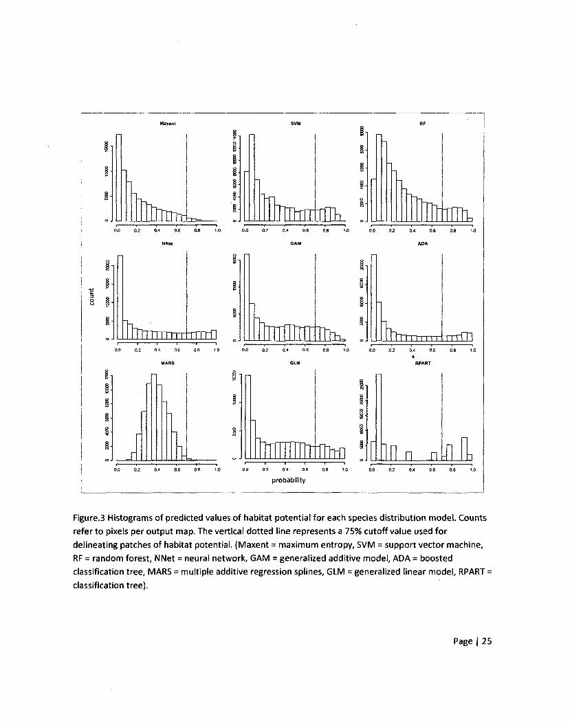
Even though some SDM's have similar accuracy values, such as MARS (AUC = 0.842, TPR = 0.684)
and GAM (AUC = 0.828, TPR = 0.686), the distribution of probability values they predict varied widely
(Figure3). The histogram for MARS showed a normal-type distribution of probability values with a slight
positive skew whereas the histogram of the GAM model showed a much more strongly skewed
distribution. Also, even though the maximum entropy model had the lowest accuracy values from both
AUC and TPR, its distribution of probability values was similar to other SDMs of high accuracy (e.g.,
boosted tree (ADA), random forest (RF)) compared to other models, such as MARS and classification
tree (RPART). This indicates that SDMs of similar model accuracy can possess very different patterns of
predictions given the same inputs.
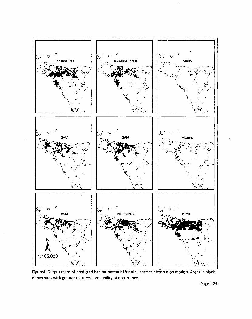
Each SDM provided a map of probability values that can be used as a surrogate for predicted
habitat potential (Guisan and Zimmermann 2000) for the eastern massasauga rattlesnake in the upper
Bruce Peninsula region. A common use of SDMs in conservation strategies is to delineate areas of high
Page | 17

habitat potential to focus on during planning initiatives. A requirement to delineate these areas is to
classify the probability image based on some threshold value. This threshold identifies how high a
probability an area must have before it is considered as habitat potential. There is no single correct
threshold value and the value may change depending on the intended application of the SDM and how
decision makers weigh true positive rates versus false positive rates. In this example a 75% probability
(0.75) value was used to delineate areas of predicted high habitat potential (Figure4). The dotted
vertical line in the histograms depicted in figure 3 shows how the habitat potential maps in figure 4
would change as the threshold value of 0.75 is changed. If the threshold value were changed up or down
a certain number of pixels would be added or subtracted from the map of each SDM according to the
distribution in figure3. Since the probability values of each SDM were positively skewed the range of
likely threshold values that would be used for conservation strategies would have a relatively small
effect on the map of delineated habitat potential.
The spatial pattern of predicted high habitat potential for six SDMs were fairly similar (boosted
tree, random forest, GAM, SVM, GLM, and neural network) (Figure4). MARS, maximum entropy
(Maxent), and classification trees (RPART) show spatial patterns that are different. These spatial
differences were not reflected by measures of model accuracy which indicates that assessing accuracy
alone may not be sufficient to determine the usefulness of a SDM for a particular conservation strategy.
To identify areas of model agreement and disagreement, maps of predicted high habitat
potential from all SDMs were summed (Figure5). Areas where most or all models (7 to 9 models) overlap
indicate sites with a relatively high level of agreement in predicted habitat potential. Areas where very
few or no models overlap (3 models or less) also indicate areas of a relatively high level of agreement
although in this case the agreement indicates a lack of habitat potential. Areas in-between, sites where
approximately half the models predict habitat potential and the other half does not (4 to 6 models agree
Page | 18

only), can represent sites with the greatest SDM uncertainty and areas that may be given special
consideration when considering conservation decisions.
Discussion
Results show that different measures of model usefulness can lead one to varying conclusions
about model selection for SDMs. Based on a threshold-independent measure of model accuracy, such as
AUC, all nine SDMs provide fair to good predictions based on independent test data. When a threshold-
dependent measure of accuracy is used however, such as TPR, not all models are deemed to give
accurate predictions with some SDMs providing predictions similar to, or only moderately better than,
random chance. These varying results provide an example of how threshold-based and non threshold-
based measures of accuracy can lead to different conclusions as to the merit of a model. Depending on
the intended use of the SDM, different types of model errors may have different costs and more than
one type of model error may be important for a planning decision. Therefore, decisions based on SDMs
should be informed by a range of accuracy measures that are sensitive to the different types of errors
inherent in any SDM. Researchers involved in SDMs are becoming increasingly aware of the limitations
of threshold-independent measures of model accuracy, such as AUC (Lobo etal. 2008), particularly
when decisions based on these models are needed.
Differences in measures of model accuracy do not necessarily reflect differences in the spatial
patterns of the predictions made by SDMs. Six SDMs provided predictions of similar spatial pattern:
boosted tree, random forest, generalized additive model, support vector machine, generalized linear
model, and neural network. However, TPR values for these six models varied from 0.686 to 0.864.
Models based on multiple additive regression splines, maximum entropy, and classification tree
Page | 19

provided quite different predicted patterns. For a conservation application whose objective is to
delineate areas of high habitat potential for use in regional management planning these three SDMs are
less useful compared to the other six. The multiple additive regression spline and maximum entropy
models estimate a much smaller predicted area than the others identifying fewer areas for conservation
opportunities. The classification model, due to the binary splits identified in the recursive partitioning
process of the RPART algorithm, creates a very artificial looking spatial pattern of predictions that is
influenced by the spatial polynomials entered into the model. These spatial patterns are unique to the
classification tree model and are not corroborated by any other SDM.
As more research is conducted into how different model types and measures of model accuracy
perform, it is becoming increasingly clear that the development and use of SDMs should not rely on a
single modeling method or accuracy measure (Liu et al. 2011). With the same input data, different SDM
methods can generate models with quite different spatial patterns in their predictions and these spatial
differences are not necessarily reflected in model accuracy measures. Where possible, multiple
modeling approaches and accuracy measures that explicitly incorporate different types of model error
should be used in an ensemble approach to inform decision making.
Page | 20

Table 1. Selected predictor variables representing habitat pattern (amount, configuration), topographic
pattern, and spatial covariates.
Label Variable Unit Description
CAforest Class area for forest per
window
ha Measure of habitat amount. Massasaugas in the Bruce Peninsula region have been known to
occur in a range of coniferous, deciduous and mixed forest types. Open canopy and forest
edge areas are preferred as they provide a range of thermal conditions. Areas of closed
canopy are avoided.
AREAwetland Mean patch area for
wetland per window
ha Measure of habitat amount. Massasaugas are associated with a range of wetland types
including swamps, fens and bogs. Wetlands are especially important for seasonal habitat
use and are often used as hibernacula where individuals can move below the frost line.
PR Patch richness of all cover
types per window
# patches Measure of habitat configuration. Massasaugas are habitat generalists and utilize a range of
land cover types throughout the active season. Accessibility to a range of resource
conditions is important for seasonal shifts in habitat use.
NPforest Number of forest patches count
per window
PARAwetland Mean patch perimeter to m / m2
area ratio for wetlands per
window
Measure of habitat configuration. Areas with a high number of forest patches are associated
with increases of forest edge which are preferred by massasaugas for thermal regulation.
Measure of habitat configuration. Massasaugas often prefer habitat edges where a range of
thermal conditions can be met in a small area.
TWI Mean topographic relative
wetness index per window index
Measure of micro-climate. Surrogate of wetness conditions at a catchment scale. Areas of
water saturation, regardless of land cover type, can be important seasonal habitat for
massasaugas, particularly for wintering sites.
TWIrng Range in topographic relative
wetness index per window index
Measure of micro-climate. Surrogate for the range in wetness values in a localized area.
Areas that provide a range of wetness conditions may be preferred by massasaugas as they
may provide a range of basking and hibernating sites in a small area.
HLI
HILrng
Mean heat load index per relative
window index
Range in heat load index relative
per window index
Measure of micro-climate. Estimate of potential direct incident solar radiation. Effected by
topographic aspect and slope. Massasaugas may prefer areas of high solar radiation as
basking sites in order to meet thermoregulation needs.
Measure of micro-climate. Estimates the range in potential direct incident solar radiation in
a localized area. A surrogate for thermal gradients needs for thermoregulation.
X
Y
X2Y
UTM Easting
UTM Northing
(UTM Easting)2 * UTM
Northing
meters Measure of spatial pattern. Spatial polynomial,
meters Measure of spatial pattern. Spatial polynomial,
meters Measure of spatial pattern. Spatial polynomial.
Page | 21
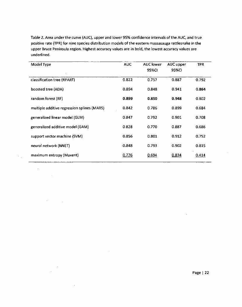
Table 2. Area under the curve (AUC), upper and lower 95% confidence intervals of the AUC, and true
positive rate (TPR) for nine species distribution models of the eastern massasauga rattlesnake in the
upper Bruce Peninsula region. Highest accuracy values are in bold, the lowest accuracy values are
underlined.
Model Type AUC AUC lower AUC upper TPR
95%CI 95%CI
classification tree (RPART) 0.822 0.757 0.887 0.792
boosted tree (ADA) 0.894 0.848 0.941 0.864
random forest (RF) 0.899 0.850 0.948 0.802
multiple additive regression splines (MARS) 0.842 0.786 0.899 0.684
generalized linear model (GLM) 0.847 0.792 0.901 0.708
generalized additive model (GAM) 0.828 0.770 0.887 0.686
support vector machine (SVM) 0.856 0.801 0.912 0.752
neural network (NNET) 0.848 0.793 0.902 0.815
maximum entropy (Maxent) 0.776 0.694 0.834 0.414
Page | 22

e
National Park
A
Canada
Study Area
USA
Figure 1. Upper Bruce Peninsula region in Ontario, Canada.
Page | 23

m
1:240,000
Legend eastern massasauga rattlesnake occurrences o- '
Figure 2. Eastern massasauga rattlesnake occurrence records in the upper Bruce Peninsula region.
Page | 24
Maxent
Mir IQL 0.0 0.2 0.4 0.6 0.8 1.0 0.0 0.2 0.4 0.6 0.6 1.0 0.0 0.2 0.4 0.6 0.8 1.0
TTTTTr n TTTTfl Qlir n u n xDH r - i" i 1 1 » 0.0 0.2 0.4 0.6 0.8 1.0 0.0 0.2 0.4 0.6 0.B 1.0 0.0 .0.2 0.4 0.6 0.8 1.0
\L
8 -i
rrmTrn i i
n n a 0.0 0.2 0.4 0.6 0.8 1.0 0.0 0.2 0.4 0.6 0.8 1.0 0.0 0.2 0.4
probability
Figure.3 Histograms of predicted values of habitat potential for each species distribution model. Counts
refer to pixels per output map. The vertical dotted line represents a 75% cutoff value used for
delineating patches of habitat potential. (Maxent = maximum entropy, SVM = support vector machine,
RF = random forest, NNet = neural network, GAM = generalized additive model, ADA = boosted
classification tree, MARS = multiple additive regression splines, GLM = generalized linear model, RPART =
classification tree).
Page | 25
Boosted Tree
-h - <7
GAM
y V** * -/? <\? ° "Or. J e °^0/
14. -v « 0 j
c £?
X * ' < 2? '
0 0 0
<7
GLM
<&• -
?i - 57
Random Forest
Y vs*-tlcSrV v , J
( /c?v.
\ £.
% 0 k 0 0
VH.
9 »
SVM
& **•
. » /
Neural Net
V
MARS
Maxent
c^o"7 w"= 5-A
•;'V /
iM
RPART
Figure4. Output maps of predicted habitat potential for nine species distribution models. Areas in black
depict sites with greater than 75% probability of occurrence.
Page | 26

Model Agreement
Legend
high agreement (no habitat potential)
m| low agreement (potential uncertain)
I J high agreement (habitat potential)
Figure5. Areas of relative high and low agreement in predicted habitat potential across nine species
distribution models.
Page | 27
Chapter 2—Multi-Causal Explanations and Severe Tests: Philosophical Contributions to Landscape
Ecology
Introduction
The discipline of philosophy of science is an active discipline with significant contributions to
make to the practice of science. Contemporary ecological literature cites the contributions of Piatt
(1964) and Popper (1934) fairly regularly (Quinn and Dunham 1983, Oksanen 2001, Davis 2006);
however, contributions from more recent philosophers (e.g., Woodward 2003, Mayo 2004) seem to
receive less attention. This also seems true in the landscape ecology literature.
Landscape ecology is "the study of how landscape structure affects (the processes that determine)
the abundance and distribution of organisms. In statistical parlance, the "response" variables in
landscape ecology are abundance / distribution / process variables, and the "predictors" are variables
that describe landscape structure." (Fahrig 2005). To reiterate from this definition we can summarize
that landscape ecology seeks to find explanations regarding the following:
• What elements of landscape structure (e.g., habitat amount and configuration) cause patterns in
species abundance or distribution? (e.g., Villard et al. 1999, Houlahan and Findlay 2003, Radford
et al., 2005, Betts et al. 2006, Rizkalla and Swihart 2006, Ritchie et al. 2009, Ethier and Fahrig
2011)
• What are the processes that determine species abundance or distribution and how does
landscape structure affect them? What are the types, directions, and shapes of these
relationships? (e.g., Robinson et al. 1995, Luck et al. 2003, Lampila et al. 2005, Hinam et al.
2008, Zitske et al. 2011)
Page | 28

• What are the things that influence the landscape structure—species abundance / distribution
relationship (e.g., spatial and temporal scale, matrix quality, habitat amount, species traits,
sampling design, analysis strategy, confounding factors, selected predictors, etc.)? (Dunford and
Freemark 2004, Ewers and Didham, 2006, Eigenbrod et al. 2011, Smith et al. 2011)
This, of course, is not an exhaustive list of the things that landscape ecology concerns itself with but
much of the current focus in landscape ecology is centred on aspects of the above points. What can the
philosophy of science contribute to the seeking of these types of scientific explanations? Much of the
philosophy of science speaks to the nature of explanations. What distinguishes a good explanation from
a bad one? How does one evaluate the truth of an explanation and how should these evaluations affect
how science is conducted? These philosophical contributions are highly relevant, especially in light of
some of landscape ecology's unique challenges, such as difficulties in designing controlled studies with
sufficient landscape replicates and logistics pertaining to manipulating landscape patterns to examine
effects at multiple scales.
The purpose of this paper is to discuss some salient points in the current philosophy of science
literature within the context of landscape ecology. Arguments made in the philosophy literature
regarding the creation of scientific understanding will be reviewed and applied to the current practice of
landscape ecology. Based on these arguments some potential weaknesses of landscape ecology will be
identified and suggestions on how to strengthen the practice of landscape ecology will be made. As a'
starting point we will expand upon what scientific explanations are and some of their attributes.
Page | 29

What is a Scientific Explanation?
Scientific explanations are descriptions of objective dependency relations between things
(Raerinne 2010). More simply put, an objective dependency relation is a "cause". So when a landscape
ecologist is studying the effects of landscape structure on the distribution of wildlife they are testing to
see if landscape structure is a cause, or more precisely part of a causal chain, that explains why a species
is distributed the way it is. Scientific explanations are often, if not always, causal (Salmon 1998). If the
purpose of scientific explanation is to gain understanding by discovering causes of phenomena, then
what is it to be a "cause"?
Causation is the relationship between an event (the cause) and a second event (the effect),
where the second event is understood as a consequence of the first
(http://en.wikipedia.org/wiki/Causalitv). A causal factor is necessary if it is a non-redundant element
needed to bring about the effect. Without its necessary causal factors, an effect will not come to be. In
the case of multi-causal relationships some causal factors may be unnecessary because the effect may
come about through some other factor (Mackie 1965, Hilborn and Stearns 1982). A causal factor is
sufficient if it is all that is needed to bring about the effect. A causal factor may be very important to an
explanation but insufficient if other causal factors are also required to bring about the effect (there is an
interaction between two or more factors) (Mackie 1965, Hilborn and Stearns 1982). A simple diagram
illustrates the difference between necessary versus sufficient preceding conditions. Figure 1 shows four
panels that are abstractions of a causal relationship between A, B, C, H and Z In panel 1, three factors,
A, B and C, are needed to bring about the effect, Z. In this case, A, B and C are all necessary but
insufficient causal factors of Z. They are all necessary because they are all needed to cause Z but
insufficient because none of them can bring about Z on their own (A, B and C all interact to cause Z). In
panel 2, either/l or B or Ccan bring about Zon its own. In this case, A, B, and C are all unnecessary but
Page | 30

sufficient causal factors of Z. Unnecessary because Z can still occur without the individual effects of any
one factor, given that at least one of the other factors are present, and sufficient because any factor, by
itself, can bring about Z. Panel 3 introduces the concept of distal versus proximate causes. Here, H is also
a causal factor of Z but its influence is only through acting on A. In this case, H is an indirect cause and is
a more distal causal factor of Z com pa red to A, B, or C. Panel 4 shows a simple scenario where A is both
a necessary and sufficient cause of Z because A alone is needed. In all these panels note that A, B, C, and
H are all preceding conditions of Z. So while A and Z are correlated in all three panels, A is a cause of Z
and not the other way around on account of /*'s preceding condition. Correlations are symmetrical
whereas causes are always asymmetrical.
This characterization of causal relationships does not require that causal factors always bring
about their effects in order to be considered a cause (Salmon 1998). This is especially true in ecology
where not all of the processes that act upon ecological phenomena across spatial and temporal scales
can be identified and measured. It may be that some elements of nature are not completely
deterministic and a random component of an effect is always present even if we have identified a
complete causal explanation (i.e., Species occurrence: A complete causal explanation may exist that
describes why an area provides suitable habitat and can support the occurrence of a species but the
habitat is currently unoccupied at a given point in time). It is therefore adequate in some cases that
causes can be identified by simply increasing the likelihood of the occurrence of the effect (Salmon
1998, Woodward 2003, Achinstein 2005).
Within a causal framework, the kinds of explanations that landscape ecology tries to find
generally have some common characteristics that are important for researchers to recognize. One
characteristic is that the mechanisms that bring about patterns in species distribution and abundance
are always multi-causal (Pickett etal. 1994). This is not a very controversial statement and is supported
Page | 31

from the theories of island biogeography and meta-popuiation dynamics where it is predicted that
landscape structure affects habitat amount and configuration that, in turn, can affect species dispersal,
colonization rates, and competition which, in turn, affects the distribution and abundance of
populations (Hanski 1999). Since the focus of landscape ecology research is in multi-causal ecological
relationships then, in order to create valid scientific explanations, it is necessary to distinguish when
causal factors created from landscape structure, if they exist, are necessary and/or sufficient.
Another common characteristic of explanations in landscape ecology is that the effect of
landscape structure on the distribution or abundance of species is always distal. Since landscape
structure often operates at larger scales than population dynamics (Allen and Hoekstra 1992), the
causes of interest are never in direct "contact" with the effects landscape ecologists are typically
interested in. Rather, landscape structure operates through more proximate causal processes that are in
closer "contact" with the distribution and abundance of populations. For example, an attribute of
landscape structure may be the amount of edge along a patch of forest. Changes in the amount of forest
edge may be a cause (though not a necessary or sufficient cause) of increased predation rates which in
turn may be a cause (also not necessarily a necessary or sufficient cause) of a decrease in abundance of
a prey species. In this example, landscape structure is a distal cause of species abundance acting through
its influence on predation rates. Moreover, since the potential influence of landscape structure occurs at
large spatial and temporal scales it may provide a context within which many species interactions
operate. Given this contextual relationship landscape effects may not be linear but rather limiting
(O'Connor 2001).
This presents some problems for landscape ecology in that potential explanations under study
will very often represent insufficient but Necessary parts of a condition which is itself Unnecessary but
Sufficient for the result. These types of causal statements are referred to in the philosophy of science
Page | 32

literature as INUS conditions (Mackie 1965). Consider the idealized example in figure 2. Here Z
represents the abundance of some population of wildlife. Changes in Z may be caused by A which, in this
hypothetical example, represents colonization rates among individual populations in a meta-population
(however, changes in Z may also be caused by other causal factors such as food availability or predation
rates, represented by 8 and C respectively). A, in turn, is caused by a range of factors such as inter-patch
distance among populations (H), matrix quality (/), and dispersal ability (J). In this example, the
relationship of the landscape attribute, H, on Z is that of an INUS condition. H is an insufficient but
necessary part of a condition (A) which is itself unnecessary but sufficient for the result Z. INUS
conditions pose a potential problem for landscape ecology because the measurement of their indirect
and distal effects may be hampered by compounding process variability, measurement error and model
error involved in quantifying relationships at each step of the causal chain (variability and errors occur at
H, A and Z). In the real world, we do not know all of the factors between the potential indirect cause of
landscape structure and the distribution and abundance of species. These unknown and unmeasured
factors may confound or mask a potential causal relationship between landscape structure and species
distribution / abundance leading to a prevalence of spurious results (Raerinne 2010).
Qualities of Explanations
Scientific explanations are often concerned with defining causes of phenomena where individual
causal factors may be necessary and/or sufficient. These causal factors may directly or indirectly bring
about, or increase the likelihood, of the effect. However, it is common in science that there exists a set
of competing hypotheses or potential explanations that attempt to explain the same phenomenon. How
should these competing explanations be compared and on what criteria should their quality be
Page | 33

assessed? This question is the focus of much attention from philosophers (Salmon 1998, Woodward
2003, Achinstein 2001, Achinstein 2005). Common attributes of powerful explanations in science relate
to non-sensitivity, precision, and factual accuracy (Ylikoski and Kuorikoski 2010).
Non-sensitivity, sometimes referred to as invariance, pertains to the range of background
conditions across which an explanation continues to hold (Ylikoski and Kuorikoski 2010). Non-sensitivity
can also refer to the range of values that the causal factors can have without breaking the causal
relationship with the effect (Ylikoski and Kuorikoski 2010). Basically, an increase in sensitivity makes the
explanatory relationship more fragile, whereas a decrease in sensitivity makes it more robust because it
is invariant across a wider range of conditions. Explanations that are highly sensitive to changes in
background conditions can be an indicator that some important causal factors are missing from the
explanation and the explanation fails to hold across these conditions because these factors are present
in some instances but missing in others. It is also possible that explanations are highly sensitive, not
because of a deficiency in the explanation, but rather due to an attribute of the thing to be explained. A
phenomenon may not be completely deterministic and its causal factors may not always bring about an
effect. In landscape ecology, both of these issues may come into play. It is easy to conceptualize how
species abundance or distribution could be caused by a very large number of potential factors that
operate at a range of scales (e.g., genes that express themselves as phenotypes causing larger body size
or tolerance to wider ranges of climatic conditions, differences in movement behaviour among
individuals in a population that may cause differences in the likelihood of gap crossings, intra-species
specific competition for spatially limited resources, variation in core habitat area among a landscape
mosaic of habitat patches in a hostile matrix). Differences in species abundance or distribution are also
likely influenced by abiotic factors (e.g., soil and water chemistry) and the history of antecedent
conditions that allowed species populations to locally adapt to available conditions. It is conceptually
Page | 34

and logistically intractable to include all these potential causal factors in a landscape ecology study. It
also seems likely that patterns in species abundance or distribution are not completely determined by
their causal factors and that some random element contributes to these patterns (Pickett et al. 1994).
As a result it should be understandable and expected that most explanations in landscape ecology are
sensitive and only hold across limited background conditions. This issue may be one of the reasons why
the effects of landscape fragmentation on species abundance and distribution seem variable across
studies (e.g., Trzcinski et al. 1999, table 1 in Smith et al. 2011). Due to these issues it may be that only
rough comparisons of explanations, based on sensitivity, can be made because not all background
conditions are equally important and the importance of background conditions may change as
circumstances change (Ylikoski and Kuorikoski 2010).
The precision of an explanation refers to how complete the explanation is with respect to
containing all of the causal factors that give rise to an effect (Ylikoski and Kuorikoski 2010). An
explanation may not be precise because it may be missing some aspects of a complete causal
relationship. The precision of an explanation, therefore, is related to its sensitivity. There is often a
trade-off between sensitivity and precision. The sensitivity of an explanation is often increased when its
precision increases. This is simply because smaller deviations are needed to disrupt the dependency
between the causal factors (predictors) and a fine-grained effect (response) than coarser-grained ones
(Ylikoski and Kuorikoski 2010). Relationships between landscape pattern and species abundance and
distribution can be imprecise because ecosystems are complex, open systems where phenomena are
affected by processes that occur at a range of scales and a range of levels of ecological organization
(Allen and Hoekstra 1992). Interaction effects are ubiquitous in ecosystems making ecological
explanations, by definition, multi-causal. Given this complexity, many background conditions will always
Page | 35

be excluded from study and true causal factors will always be left out of any explanation in ecology for
conceptual and logistical reasons.
Factual accuracy is another means by which one can assess the quality of an explanation.
Factual accuracy refers to the notion that truth is not "all or nothing" but rather can be thought of as a
gradient in that an explanation can be generally true but still contain some falsehoods (Ylikoski and
Kuorikoski 2010). While it is true that false explanations would generally lead to false answers, some
explanations may contain mostly factual relationships but still possess some incorrect causal factors.
Examples of falsehoods may be the wrong set of predictors (causal factors) in a model or the correct set
of predictors but the wrong estimated relationship between the predictors and the response (e.g., linear
versus non-linear). Another type of falsehood can be the incorporation of idealizations or surrogates
into an explanation in order to make the explanation more tractable or easier to measure (Ylikoski and
Kuorikoski 2010). Landscape ecologists often use surrogates in their explanations such as the use of land
cover types (e.g., forest) as a surrogate for habitat or patch size as a surrogate for resource availability
(Lindenmayer and Fischer 2006). These kinds of idealizations are necessary due to the scale of
investigation and the fact that individual landscapes are the sampling unit. Detailed field measurements
of the multivariate aspects of species-specific habitat or resource availability replicated across several
landscapes, each of which containing many patches or habitat units, are usually not feasible from a
logistical perspective. In these cases, the use of idealizations allows scientific study to continue even
though these surrogates may introduce factual inaccurate statements into explanations provided by
landscape ecology. While these explanations may contain some falsehoods, they still may provide
explanations that consistently lead from their causal factors to their effects in a way that is non-sensitive
and precise enough to be informative and useful.
Page | 36

Evaluation of Common Landscape Ecology Explanations
Now that certain key ideas about how the philosophy of science views scientific explanations
have been introduced, we turn our attention to how these ideas can help evaluate some common types
of explanations in landscape ecology. In this section, some key questions in landscape ecology will be
reviewed in light of these ideas regarding explanations and causal relationships.
Scale Dependent Effects of Landscape Structure
It is recognized that the relationship between landscape structure and the distribution and
abundance of species can be scale dependent (Fahrig 1998). As scale changes, different landscape
elements may become more or less important and the magnitude and even the direction of effect may
change (Krawchuk and Taylor 2003, Smith et at. 2011). Due to these scale dependencies there may be
critical scales of influence (i.e.: scale of effect) where species respond most to patterns in landscape
structure (Ethier and Fahrig 2011). A common approach to studying the scale dependent effects of
landscape structure is to quantify the pattern of landscape structure at different spatial scales around
focal patches that are surveyed in terms of a species' abundance or occurrence (Figure 3); (Brennan et
al. 2002). The relationship between landscape structure and species distribution or abundance is usually
measured through some kind of regression model and the magnitude of scale dependency in these
relationships are quantified by comparing the R2 or AIC values among models created using the same
predictors measured at a range of scales around the focal patch.
What may be the quality of these kinds of explanations concerning the scale dependent effects
of landscape structure? Consider the following: entities in nature (e.g., individuals, populations,
resources, habitats) are rarely distributed in a homogeneous or completely random manner. They tend
Page | 37

to have some kind of spatial pattern or clustering at some spatial scale(s). If this is true then as the size
of area around any focal patch is changed some change in spatial pattern would also be expected,
though the change may be large or small. Study design may influence the magnitude of this change but
some change in spatial pattern will occur. If the patterns change across scales then the parameters in a
regression model (e.g., partial regression coefficients) must also change because the values in landscape
predictors will change. If the parameters among regression models change then so must measures of
model fit (e.g., R2 or AIC). If these measures change then there will always be a scale that possesses the
highest R2 or lowest AIC. This must be true if for no other reason other than they will not all be the
same. Therefore, when approached in this way, "critical" scales will always be detected whether the
species actually responds in a differential way to patterns at that scale or not. Put another way, critical
scales will always be detected based solely on the function of changing pattern in the landscape as scale
changes and not necessarily due to any behavioural response from the species. In these cases, the
likelihood of spurious results is high.
This problem becomes compounded when landscape ecologists study the effects of landscape
structure using a range of predictors (e.g., measures of amount, shape, edge, isolation, matrix quality),
across multiple species, using varying model types (e.g., generalized linear models, generalized additive
models, tree models), and assessed at a range of scales (Betts et al. 2006). Given that nature always
contains some kind of spatial pattern, the investigation of these many conditions (predictors X species X
model types X scales) will most certainly detect some kind of effect based on overlapping spatial pattern
even if the results are completely spurious. In these cases finding no statistically significant relationship
at all may be more surprising than finding at least one "significant" result across so many combinations.
A critical question regarding these types of studies is how sensitive is the detection of critical
scales of effect to changes in background conditions? If studies were replicated in different but similar
Page | 38

areas such that the sampling strategy, species response variables, landscape predictors and analysis
method were the same, how would this affect the detection of scale effects? Here the concepts of
sensitivity and precision are useful to determine how strong the explanation of scale dependent effects
is. Studies could initially be replicated in neighbouring areas to the original study where changes to
background conditions are likely to be the smallest. The two sets of analyses would be very similar with
only the changes in background condition being different. If the inputs across these two studies were
similar then so too should be their detected scales of effect. Similar but not necessarily identical and so
small differences may be allowed among the critical scales to still stand as being consistent (a less
precise explanation is accepted to account for differences in background condition). If the explanation
put forward in the original study were true then the scales of effect should be similar. If they are not
then it is possible that the results of the first study are spurious. If results are confirmed across these
two studies then it could be replicated further in areas farther away from the original study and changes
in important background conditions could be measured across each replicate. The more consistent the
results are across replicates (increasing number of confirming instances of the explanation) the more
support the explanation will have. If the results fail under some set of replicates with different
background conditions then it may be that those specific background conditions are important, but
previously unknown, elements of the explanation. These specific conditions could then be incorporated
into a refined explanation and new knowledge will have been gained. Of course, a challenge of
landscape ecology is that, given the large spatial scales of study, it is logistically difficult to replicate
studies. A simpler starting point, then, may be to partition the original dataset into spatially non-
overlapping areas that are large enough to contain enough focal patches and their largest scale of study
and still have enough degrees of freedom to support the method of analysis. If results across partitions
are consistent it could be concluded that the detected scales of effect are, so far, deemed to be non-
spurious.
Page | 39

In addition to the concepts of the sensitivity and precision of an explanation, this approach also
incorporates two other ideas: (1) that attributes of background conditions are an essential part of a
scientific explanation and, to the extent possible, should be measured and explicitly incorporated into
the explanation, and (2) that the number of confirming instances of a model provides increased support
for the explanation and gives more information regarding the range of contexts in which the explanation
holds or does not hold. Explanations that are only supported by the data used to generate the initial
model do not count as an independent confirming instance and provide very little support.
One way ecologists try to determine the sensitivity of explanations involving the effect of
landscape structure on species is through meta-analysis. Meta-analyses are syntheses where results
across studies are compared with respect to their observed effects sizes in relation to their attributes
(e.g., sample size, variability around reported results, study design elements). However, if models from
individual studies in landscape ecology are not evaluated beyond the data used to create them, and the
quality of their explanations are low and their results unknowingly spurious, then meta-analyses that
use these published papers could be biased as they would equally weigh results from studies regardless
of the quality of explanations they report. One way to address this could be to give higher weight to
results from studies that employ some strategy of testing their models beyond their original training
data (e.g., testing model prediction against a separate random data partition).
Relative Importance of Independent Effects of Landscape Pattern
A common approach to assessing the relative importance of effects of landscape pattern (e.g.,
habitat amount versus composition versus configuration) is to use statistical models to determine the
independent effect a predictor variable has on a response variable such as species abundance or
Page | 40

distribution (Smith et at. 2011). Statistics are used to isolate the effects of one predictor in a statistical
model through parameters such as partial regression coefficients that estimate the magnitude of effect
t
of one predictor variable while keeping other predictors constant (Smith etal. 2011). Some philosophers
of science contend that statistics are not a tool to illuminate the truth of potential scientific explanations
(Sober 1988, Ylikoski and Kuorikoski 2010). What statistics do, they contend, is simply describe the
relationships between a set of variables within a given model and how likely that relationship would be
if the variables were random and the study replicated a very large number of times. A regression
equation such as y=3.2+6.7x1+2.1x2, P=0.04, R2=0.5, describes the relationship between Xi, X2 and Y
given the particular set of data used to construct the regression model. It does not say anything
regarding the extent to which Xi and X2 are relevant causal factors of Y and, therefore, the regression
equation, by itself, does not represent an explanation, only a description. The assumptions made by this
regression equation include that the relationship between the predictors and response is a linear mean
relationship and that the independent effects of the predictors are additive (Ylikoski and Kuorikoski
2010). These untested assumptions are properties of the statistical model and may have no bearing on
the real casual system under study.
Statistical measures of relative variable importance are only relevant insofar as the statistical
model is relevant and represents an adequate explanation of the phenomena of interest. The regression
equation given above would have more bearing on an explanation if the study were replicated in
different background conditions and the relationships between Xi, X2 and Y were invariant across a
range of separate and joint manipulations of X* and X2. From these replications the researcher would
have more information as to whether the relationships between the variables in the equation were
factually accurate and whether the regression coefficients were highly sensitive to background
conditions. These issues, however, are not statistical but rather pertain to an overall research strategy
Page | 41

that more deeply probes the relationships between X1( X2 and Y (Mayo 1991, Mayo 2004, Mayo and
Spanos 2006).
Gaining Support for an Explanation in Landscape Ecology through Severe Tests
The previous discussion of types of studies in landscape ecology highlights some key points
regarding scientific explanations that may be useful for the field of study. The focus of explanations is to
find causal relationships. When landscape ecologists try to find explanations of patterns of species
abundance or distribution they are attempting to identify under what conditions is landscape pattern a
causal factor. Landscape pattern, if it is a causal factor at all, will likely be part of a multi-causal
relationship as many ecological processes at a range of scales affect species abundance and distribution.
Within these multi-causal relationships landscape pattern may be necessary or unnecessary, sufficient
or insufficient to cause changes in species patterns. If landscape pattern is a true causal factor it will
likely be an INUS condition. Also, because so many complex and interacting factors can affect species
patterns, they cannot all explicitly be part of a causal relationship under study as this would make
research conceptually and logistically intractable. Simplifying assumptions, implicit or explicit, will
always be part of landscape ecology research. As a consequence, explanations in landscape ecology will
likely be sensitive to changes in background conditions because these conditions will contain many
unmeasured causal factors.
How can landscape ecologists use this information to improve the quality of their research? Two
conceptually straightforward actions are suggested, though their implementation may not be so
straightforward in practice. First, landscape ecologists could focus more on response variables that are
more proximate to potential causal factors involving landscape structure. If it is known a priori that
Page | 42

landscape structure potentially affects species abundance through ecological processes such as
dispersal, increased mortality in the matrix, decreases in resources with losses in habitat amount, then
these processes could become our explicit response variables. By focusing on response variables that
are more proximate to potential landscape causal factors identified relationships may be more readily
detected and consistent across studies. While many landscape ecology studies already do this, often the
response variables are simply species abundance or distribution and these processes are inferred post
hoc to explain why a certain pattern was detected in their data. Also, since explanations in landscape
ecology will likely relate to multi-causal relationships efforts could focus on more complex hypotheses
than independent individual effects of habitat amount, composition or configuration. Due to the
exclusion of many potentially important causal factors that are implicitly included as unmeasured
elements of a study's background conditions, it is also important that samples in landscape ecology
studies are sufficiently large and potential effects of background conditions are randomized.
The second suggestion pertains to the notion of a "severe test". Explanations gain support if
they continue to stand through repeated scrutiny. Whether a researcher uses a confirmation or
falsification approach, the greater the number of times an explanation can be confirmed through
repeated studies and observations or the greater the number of times it can pass an experiment without
being falsified, the more support it will have. Explanations or models that have been assessed only with
the data used to create them in the first place are very preliminary and should receive very little
support. Intuitively, an explanation that has passed repeated scrutiny from twenty studies should have
more support than an explanation that has passed scrutiny from only two studies. The explanation
tested by twenty studies is more "highly probed" than the one from two studies and deserves a greater
level of support (although this support should be tentative as the explanation from two studies may go
on to pass scrutiny from over thirty more future studies and eventually become the more highly probed
Page | 43

and successful explanation). Another way of saying this is that the explanation from twenty studies has
passed a more "severe test". Landscape ecology may be particularly prone to spurious results because:
1. controlled experiments are difficult to design due to operational logistics regarding manipulations and
replication; 2. logistics around sampling sufficient numbers of landscape units due to limited access or
land ownership; 3. many potentially uncontrolled confounding variables as part of a study's background
conditions; and 4. the fact that all resources in nature possess some kind of spatial pattern at some scale
that give rise to many correlations in landscape ecology but not necessarily explanations. To guard
against spurious results in landscape ecology more should be demanded from these studies and
potential explanations. They should pass some sort of severe test.
A severe test is no one particular type of study or analysis but rather it is a series of actions that
work towards probing the attributes (non-sensitivity, precision, factual accuracy) of our explanations
(Mayo 2004). The greater the severe test a landscape ecology explanation can pass the more support it
should receive from in and out of the discipline. While other landscape ecologists can no doubt devise
many different kinds of severe tests, a severe test is suggested with a simple set of steps that could go a
long way in reducing the prevalence of spurious results in landscape ecology. This proposed severe test
has 4 steps (Table 1).
The first step pertains to model fit. If a statistical model is to provide a suitable explanation then
it should fit the initial data (training data) well. The specific measures of model fit will vary depending on
the type of question asked and the specific model types used in analysis. Also the degree of fit may be
flexible depending on the situation. There is no single correct minimum standard for model fit. The idea
is that measures of model accuracy, and the level of acceptable accuracy that qualifies as a potential
explanation, should be identified ahead of time. Only after this step has passed should a candidate
model proceed to other steps of this suggested severe test.
Page | 44

The second step refers to model accuracy. Accuracy here should be assessed through the use of
independent random partitions of the training data. Since these partitions are randomly selected across
the original study area they should roughly possess the same background conditions but will differ
slightly in terms of patterns within the data. If a model represents a true explanation, and if the
background conditions do not change in a meaningful way, then the model should fit random data
partitions well. The number of random partitions to be compared with the training data will depend on
study logistics and sample size. The message here is that models should be compared to independent
data and random partitions of the original dataset represents the least severe comparison since they
should contain the same background conditions. If the model fits the training data well but not
independent random partitions from the same background then this is an indication that the model is
spurious. Some landscape ecology studies go to this step (e.g., MacLeod et al. 2008) but these studies
are in the minority.
The third step we will call model replicability. Here the model that represents a potential
explanation should be applied to other areas outside of the original study area such that background
conditions vary. The models could be replicated at neighbouring sites where background conditions, due
to spatial autocorrelation, will likely change the least. Models could then be exposed to areas farther
away with increasingly different contexts. For the predictor variables of interest, if the range of variation
in the values are similar to the original study area, then when the model is replicated using the new
data, the model should fit reasonably well. If it does not then it could be that the model is spurious and
holds only for the specific patterns within the training and random data partitions or that the model is
not spurious but is highly sensitive to the changes that occurred in these neighbouring areas. In either
situation knowledge is gained about the quality of the potential explanation. If the explanation is true
but highly sensitive then it may not be useful as a generalization in landscape ecology. If the explanation
Page | 45

is believed to be non-spurious then research could proceed by trying to determine what specific
background conditions were "difference makers" in causing the model to fit in one context but not the
other. This may lead to a more complete causal explanation that could then be tested by beginning back
at step 1 of this "severe test".
The fourth step refers to model consistency. It is not enough that the models fit well when
replicated across data sets that represent increasingly different background conditions. For the
explanation to be true then the story that the models tell should also be consistent. A model that fits
well in one context but shows a positive relationship between landscape structure and species
abundance compared to a model that fits well in another but similar context and shows a negative
relationship between the same variables is an indication that the model may be spurious. It may also be
an indication that the model is factually inaccurate in some way and may be missing an important causal
factor that is different in the background conditions of one area compared to the other and it is the
influence of this unknown factor that caused the relationship of landscape structure to switch from
positive to negative. Even if the explanation were true, when comparing model results from non-
overlapping areas we would expect some variation in model parameters simply due to random changes
in background conditions. So we should allow for some flexibility in the precision of these parameters.
For example, changes in partial regression coefficients, so long as they remain consistent in their
direction (either positive, negative, or not significantly different from zero), should still be taken as a
sign of model consistency. This fourth step is similar to a meta-analysis that compares model results
across studies with different background conditions. A main difference here is that, with respect to an
individual study, a model could be replicated using a random test dataset that is a subsample of the
original training data and represents the same background conditions. If the models from training and
test data are consistent then the model could be compared with data from areas adjacent to the initial
Page | 46
study area. These background conditions would likely be only moderately different from those of the
original model. If it was believed that these moderate changes in background conditions were not
critical to the explanation then the models should be consistent when compared to the original training
data. If they are not then it may be that there is some significant difference in background condition
which is an important component to the explanation or the original model may be spurious. A model
that has been tested across a range of conditions would represent a more highly probed explanation
than a model that was only assessed using the original training data. These models could be more
heavily weighted in a meta-analysis since they have passed a more severe test. Without information on
the extent to which models in individual studies were highly probed, a meta-analysis may unknowingly
incorporate spurious results that may lead to errors.
Conceptually, the 4 steps in this proposed "severe test" are straightforward. In landscape
ecology, the ability to consistently measure landscape structure across different areas is feasible due to
increasingly available remote sensing data sources. The logistical difficulty will be to sample response
variables with sufficient sample size across these ranges of background conditions. However, this
straightforward severe test allows for a landscape ecologist to do a variety of things. It allows the
researcher to assess how sensitive a potential explanation is by comparing it to data from the same
background conditions (through comparisons between the training and random partitions) and from
adjacent areas where background conditions will change but only moderately. Depending on the
objective of research, these partitions could represent a gradient of changes in specific attributes of
potential causal factors or background conditions in order to determine how these factors affect the
potential explanation. Doing so may iteratively improve the factual accuracy of the explanation. The
more times a model can be successfully replicated and shown to fit well and be consistent the more
confirming instances the explanation will attain and, therefore, the more support it should garner.
Page | 47

Conclusion
Many studies in landscape ecology seek to determine if landscape structure is a causal factor in
the pattern of species abundance and distribution. From a causal framework, landscape structure can be
thought of as an INUS condition with respect to species patterns. This means that landscape structure
will always work within a multi-causal system and that the effects of landscape structure will always be
distal to its response variable. The distal nature of these relationships mean that explanations in
landscape ecology will likely not be precise since they will be affected by error and variability from other
factors within the causal chain. Explanations in landscape ecology may also be very sensitive to
background conditions because, due to the complexity and open nature of ecosystems, many potential
causal factors cannot be explicitly included for study and their unknown effects will change as patterns
change across studies. Therefore, landscape ecology explanations may be true but still not hold across
studies due to changes in meaningful background conditions. These challenges should inspire landscape
ecologists to demand more severe tests for their models to better distinguish if model results are
spurious due to the random patterns in their data versus a potential true explanation.
The severe test proposed here may improve the quality of landscape ecology studies. Spatial
landscape patterns are ubiquitous in nature, especially when measured at a range of scales. Given the
prevalence of pattern, statistical models may identify statistically significant but completely spurious
species—environment relationships. The likelihood of spurious results increases for models that are only
assessed from the original training data. A severe test would be useful in probing the extent to which
spurious results occur and could guard against potentially erroneous conclusions.
Page | 48

Table 1. Steps in a "severe test" for landscape ecology.
Steps of Severe Test Description
1. Model fit A statistical model that represents the beginnings of a potential explanation
should fit the data used to create it (training data) reasonably well (this degree of
model fit will likely be an over estimate). Usually if an initial model does not fit
the original data then the explanation that model represents is typically
abandoned.
2. Model accuracy If a model fits the training data sufficiently then the model should be tested
against a random partition of the training data. This random partition represents
the same context as the training data and should have approximately the same
background conditions. For a model to hold it should fit this random partition as
well.
3. Model If a model fits the training and random partitions reasonably well then the model
replicability should be iteratively tested using independent datasets whose background
conditions are similar but not identical from the original. These independent
datasets may represent a spatial partition (data taken from separate location
from the original) or a temporal partition (data taken from the same location but
represents a different time period). If the model represents a valid explanation
then it should fit these similar data fairly well.
If the explanation represented by a statistical model is valid then the parameters
that comprise that model should be consistent across all data partitions.
Predictor—response relationships should have similar shapes and directions. The
precision of the explanation should be such that allows for minor deviations in
shape (e.g., smaller of larger partial regression coefficients) but the direction
(positive, negative, not differentiated from zero) of the effect should be
consistent across all partitions.
4. Model
consistency
Page | 49

Figure 1. Four hypothetical causal relationships. In panel 1, A, B and C are all necessary but insufficient
causes of Z. In panel 2, A, B, and C are all unnecessary but sufficient causes of Z. Panel 3 is similar to
panel 2 with the exception of H which is a preceding cause of A and a distal causal factor of Z. Panel 4
shows a simple case where A is both a necessary and sufficient cause of Z.
Page ( 50

M
Figure 2. A hypothetical causal explanation of Z. A, B, and C represent unnecessary but sufficient causes
of Z. Factors H through V are all INUS conditions (Insufficient but Necessary causal factors of an
Unnecessary but Sufficient condition) of Z.
Page | 51

Figure 3. An example of a focal patch approach used to assess scale dependent influences of landscape
structure of species abundance or distribution. Landscape structural variables are measured at each
scale represented by each concentric circle. The size of scale that corresponds to a regression model
with the highest R2 value or lowest AIC value is considered to be a critical scale of influence.
Page | 52

Chapter 3—Prediction and Explanations "Severe Test" for Examining the Effects of Landscape
Pattern on the Occurrence of the Eastern Massasauga Rattlesnake
Introduction
The determination of species-environment relationships is very important for wildlife
conservation. Quantification of these kinds of relationships is often relied upon to create predictive
habitat suitability maps that are used for conservation strategies and land use planning (Guisan and
Zimmermann 2000, Scott etal. 2002). To be effective it is important that habitat maps be based on
species-environment relationships that not only predict well, but also explain well and can be used over
a range of conditions that are relevant for decision making. A model that explains well should be based
on non-spurious relationships that represent true interactions between species distribution and
environmental conditions. However, as modelling methods become increasingly powerful (e.g., machine
learning), and accessibility to data on environmental variables (e.g., remote sensing) increases, the
likelihood that a habitat model is generated on spurious relationships increases. Methods for assessing
model accuracy and predictive success are available but these perse cannot distinguish between
spurious and non-spurious results.
Consider the three statistically significant (p<0.05) regression models in table 1. Model #1
represents an observed relationship between the likelihood the U.S. Presidential election will be won by
the Republican Party and the ratio of vampire to zombie movies released during the preceding
Presidential term. Model #2 represents an observed relationship between the abundance of map turtles
(Grapetemys geographica) and the proportion of grassland and shrubland in thirty five 23 km2 area
landscapes containing wetlands. Model #3 represents an observed relationship between height and
weight among 200 randomly selected people. Statistically speaking, all three of these models are valid.
The statistical models and their regression coefficients are all significant. Yet, clearly, they do not all
Page | 53

provide the same quality of explanation. For model #1, there is no logical or theoretical reason to
presume that the ratio of vampire to zombie movies affects the outcome of U.S. Presidential elections.
Despite the statistical significance most people would conclude that this relationship is coincidental and
if the model were exposed to new data this relationship would likely not hold. Model #3, on the other
hand, seems to have logical support. Generally speaking, taller people tend to be heavier. There can be
substantial variability in this relationship (i.e., there can be tall, light people and short, heavy people) but
on average this relationship holds true. Also, if we compared people's height and weight from different
parts of the world, or compared people from 1980 and 2010, we would still expect that, on average,
taller people tend to be heavier than shorter people. The height—weight relationship is consistent and
holds in different contexts.
Now consider model #2. Why would the amount of grassland or shrubland in a 23km2 area
affect the abundance of a largely aquatic species such as map turtle? Perhaps grassland and shrubland
are important upland nesting habitat for map turtle and the amount of these resources has a positive
effect on fecundity thereby increasing population abundance? Through this relationship grassland and
shrubland amount may have a positive effect on map turtle abundance. Like model #3, this rationale
gives model #2 a logical and theoretical justification. However, the effect of habitat amount on species
abundance, while usually positive (e.g., Trzcinski etal. 1999), is not always consistent. There are
examples where habitat amount effects have been shown to be significantly positive, significantly
negative, or non-significant for the same or similar species across numerous studies (Rizkalla and
Swihart 2006). So while model #2 and model #3 are similar in that they share some logical and
theoretical support, they differ in that model #3 is more consistent across multiple studies conducted in
multiple contexts.
Page | 54

This brief discussion outlines three important aspects of discriminating among models that are
likely spurious versus non-spurious. First is statistical significance and model fit. Second is the logical and
theoretical foundation of the relationships represented within the model. Third is the support the model
maintains through multiple tests and comparisons across a range of conditions (Woodward 2003, Mayo
2004). Model #1 only possesses the first characteristic. It is statistically significant but lacks logical
support and has not been subjected to multiple tests. Therefore, most would conclude that model #1 is
spurious. Model #3 possesses all three characteristics and most would conclude that the relationships
this model represents are real. Model #2 is in the "middle". It seems to possess a possible logical and
theoretical foundation but when the relationships are tested across studies that represent different
contexts (e.g., varying species, location, time, scale, study design, community composition, and
antecedent conditions) they are sometimes inconsistent. How are we to know if model #2 is spurious?
A very important point to emphasize here is that among these three models some are likely
spurious and some are not. Yet statistics alone cannot tell the difference. Measures of statistical
significance, model fit, and variable importance (e.g., partial regression coefficients) are all successfully
applied in these models. Yet, if the model itself is spurious, these statistical quantities are descriptive
only. They only describe the relationships among the variables in that model given the pattern in the
particular data set used. They are not relevant, if the model is spurious, in providing an explanation of
what causes the trends in the response variable.
Considering model #2 and landscape ecology in general, given the inconsistency in relationships
between landscape pattern and species abundance or distribution, how can we determine which
conclusions are true and which are false? Some have attempted to explain the inconsistency in results as
functions of factors not considered in the original studies such as species traits (e.g., Desrochers et al.
2010, Rytwinski and Fahrig. 2011,), selection of predictors (e.g., Fahrig 2003), or study design (e.g.,
Page | 55

Brennan etal. 2002). Yet conclusions regarding the effect of landscape pattern remain varied (perhaps
leading one to suspect that these newer findings may also be spurious). Often in landscape ecology,
when results are inconsistent across species, scales, or some other factor, post hoc explanations are
given that may account for the differences. However, if landscape effects truly are erroneous but those
effects are examined through an increasing number of combinations (e.g., species x predictors x scales),
then the mixture of inconsistent results showing positive trend, negative trend or no trend is exactly
what one would expect (results appear random with the direction of relationship occurring purely by
chance).
The field of philosophy of science is a continually evolving discipline and can perhaps provide
valuable insight as to how individual landscape ecology studies can guard themselves against potential
erroneous results. All research strategies, implicitly or explicitly, employ deductive and/or inductive
reasoning (Hempel 1965), although an inductive approach is much more common in landscape ecology.
Deduction relies upon arguments that attempt to show that a conclusion "necessarily follows" from a
set of premises. If the predicted conclusion follows the premises (or hypothesis), and the premises are
valid, then the premises must be true (Hempel 1965). Induction, on the other hand, constructs
arguments that represent a premise that proceeds from a generalization about a sample to a conclusion
about a population (Hempel 1965). Both approaches suffer from limitations. One of these limitations is
that, in nature, not every observed effect or response has 'a' cause (Salmon 1998). In ecology, an effect
may have multiple causes that shift depending on factors that are limiting in a particular context
(O'Connor 2002). Also, an effect may not be completely deterministic. Even if an effect does have 'a'
cause, the cause may not give rise to the effect 100% of the time (Salmon 1998). Hence, a single result
based on either an inductive or deductive approach cannot be definitive. Our belief, therefore, in the
truthfulness of a relationship is commensurate with the degree to which that relationship has passed a
Page | 56

"severe test" (see Chapter 2). A severe test may not be a single test perse but a range of tests and
approaches that vary across disciplines or studies. For example, following a classic inductive strategy,
one such severe test may be if model #2 were consistently replicated 10 times in varying areas of the
species range and the amount of grassland and shrubland were found to have a positive effect on map
turtle abundance 100% of the time. If this were true then model #2 would be considered to have passed
a more severe test than simply conducting the study once. Having passed this more severe test we
would be more apt to conclude that the habitat amount—map turtle abundance relationship is non-
spurious (even though our support for this model is still tentative as it may fail if replicated an 11th time).
Since model #2 is a unique observational study and has not passed a severe test, such as the one above,
our support for this model should be tenuous even though the results were statistically significant.
Model #2 represents a common occurrence in landscape ecology. Many published landscape ecology
studies are observational or quasi-experiments whose resulting statistical models are not subjected to
independent data.
The purpose of this paper is to apply this notion of a severe test to a study of the effects of
landscape pattern on the distribution of a particular species. Specifically, this paper examines the ability
of landscape-scale patterns in land cover amount and configuration to predict and explain the
distribution of the eastern massasauga rattlesnake (Sistrurus catenatus catenatus) in the upper Bruce
Peninsula region of Ontario, Canada. The ability of landscape pattern to successfully predict versus
explain the occurrence of massasaugas are kept intentionally separate since, from Chapter 1, all three
models provided adequate predictions (in that the models were able to fit patterns in the predictor
variable to patterns in the response variable) yet they all did not provide meaningful explanations.
Discriminating between models that predict well versus models that predict and explain well is very
important, particularly for Species at Risk such as the eastern massasauga rattlesnake (Chapter 1). The
Page | 57

Eastern Massasauga Recovery Plan, as part of the Canadian Species at Risk Act, is required to identify
critical habitat throughout its range, including the upper Bruce Peninsula region (Eastern Massasauga
Rattlesnake Recovery Team 2005). Given the large areas across which habitat mapping must be
conducted, remote sensing and land cover pattern data are potentially efficient and effective predictors.
Accessibility to remotely-sensed data and a large number of GIS (geographic information system) tools
and methods, however, can dramatically increase the number of predictors and models upon which
habitat maps can be derived. This increases the likelihood that erroneous habitat relationships are
"discovered" by chance causing habitat models to perform poorly when used for recovery and
management purposes. To be useful, habitat models should predict and explain well.
Methods
Focal Species and Study Area
Eastern massasauga rattlesnakes are an endangered species at risk in Canada. Their range is
described as western New York and southern Ontario extending westward to Iowa and southward to
Missouri, with zones of inter-gradation between eastern and western massasauga in south-western
Iowa and extreme western Missouri (Conant and Collins 1991). In Ontario, massasaugas are known to
occur in only four population regions: upper Bruce Peninsula, eastern Georgian Bay, Wainfleet Bog, and
Ojibway Prairie (Eastern Massasauga Rattlesnake Recovery Team. 2005). Massasaugas are habitat
generalists and occupy a range of land cover types. These include coniferous, deciduous and mixed
forests, grasslands and open fields, and wetlands. They tend to prefer open vegetated structure relative
to surrounding areas. These vegetated edges provide shaded and exposed areas that allow for a range
of thermal conditions. Thermoregulation requirements seem to drive much of their habitat selection
Page | 58

and localized thermal gradients allow individuals to meet thermoregulatory needs in a relatively small
area. Massasaugas also are associated with proximity to water saturated sites (e.g., fens, bogs) where
individuals can move below the frost line for hibernation (Johnson et al. 2000).
The study area was located within the upper Bruce Peninsula region (Figure 1). The Bruce
Peninsula eastern massasauga rattlesnake population region is one of the largest in Canada. This site
was chosen for this study because within this area is Bruce Peninsula National Park (BPNP). BPNP has
been active in managing and monitoring massasaugas in the area since its establishment in 1987. The
park maintains a database of known occurrences that have been collected through research, inventory
and long-term monitoring programs. The area was also selected for this study because it is
geographically contained by water to the north, west and east and by land conversion and human
development to the south. Therefore, land cover patterns were not truncated by imposing arbitrary
boundaries through study site delineation, which may otherwise be a source of error in examining the
relationships between landscape pattern and the distribution of the massasauga. The activity range of
massasaugas in the upper Bruce Peninsula has been estimated to be 25(±6SE) ha though a range of 0 ha
(for a gravid female) to 76.4 ha (for an adult male) (Weatherhead and Prior, 1992).
Data and Variables
The response variable for this study was the occurrence of eastern massasauga rattlesnakes.
Occurrences were evaluated based on date, spatial positional accuracy and observer. Occurrences
retained for analyses were those recorded between 1990 and 2006, were positionally accurate within
10m or less, and were recorded from experienced park staff or researchers only. These data were
partitioned four different ways: a spatial partition (spatial) that represented a non-overlapping area with
Page | 59

all other partitions (Figure 1), a temporal partition (temporal) that represented occurrences recorded
between 2004 and 2006, a training partition (training) that represented 75% of the remaining
occurrences that were recorded prior to 2004 and do not overlap with the spatial partition, and a test
partition (random) that represented a 25% random sub-sample of the remaining occurrences. During
the periods between the training partition (1990 to 2003) and the temporal partition (2004 to 2006) the
patterns of land cover, topography, land use and distribution of the eastern massasauga rattlesnake
were known to be generally stable (Parks Canada 2005). The spatial partition represented the same
general area within the upper Bruce Peninsula and the landscape pattern in terms of land cover,
topography and land use was similar throughout the study area. This partition, therefore, represented
very similar, though not identical, conditions from the training partition. The numbers of occurrences in
each of these partitions were supplemented by an equal number of randomly generated points that
represent the spatial patterns in the underlying area. Final sample sizes for these partitions were as
follows: training (n=216), random (n=76), spatial (n=122), and temporal (n=106).
The predictor variables represented landscape-scale patterns derived from a classified Landsat
TM image and digital elevation model. The classified Landsat TM image was processed as part of the
Ontario Ministry of Natural Resources and the National Imagery Coverage (Landsat 7) Project from a
mosaic of Landsat TM scenes that represented cloud free, peak phenology images from 1999 to 2001.
This 30m pixel resolution mosaic image possessed 28 land cover classes with average classification
accuracy greater than 85% (http://ess.nrcan.ec.ca/2002 2006/esdnr/success/storv2 e.php). The digital
elevation model (DEM) used was derived from a composite dataset including Ontario Base Map contour
lines. The DEM was flow corrected with an estimated 10m spatial resolution and 5m vertical accuracy
(http://lioapp.lrc.eov.on.ca/edwin/EDWINCGI.exe?IHID=4863andAgencvlD=landTheme=AII Themes).
Using ArcGIS 10.0 (ESRI 2011)and Fragstats 3.3 (McGarigal et al. 2002), predictors were derived to
Page | 60

represent a set of plausible landscape patterns that may influence massasauga distribution in the upper
Bruce Peninsula These included surrogates for land cover amount (class area, patch size, core area, total
edge, perimeter—area ratio), composition (patch richness), and configuration (number of patches,
nearest neighbour distance), and topographic pattern (elevation, slope, aspect, topographic wetness
index, heat load index, solar radiation). Predictors were derived for both forest and wetland land cover
classes. In order to control for influences of spatial auto-correlation and spatial patterns not explained
by the landscape predictors, a set of spatial polynomials were also included (Borcard and Lengendre,
2002). Values for all predictors were calculated based on a 25ha neighbourhood surrounding each
occurrence or random point that represented the mean activity range of the massasauga in the upper
Bruce Peninsula (Weatherhead and Prior, 1992). Other neighbourhood sizes were considered within the
range of massasauga home range size (0 to 75 ha), however, following a variogram and Moran's I
analysis using Passage 2.0 (Rosenberg and Anderson 2011) it was concluded that the pattern in
predictor variables across these scales were spatially auto-correlated such that predictors scaled to
these other sizes would be redundant. To account for multi-collinearity within the set of predictors, a
principal components analysis (PCA) and variance inflation factor (VIF) analysis was conducted (R 2.10.1
- http://cran.r-project.org/) in order to find a parsimonious set of non-collinear predictors that
represented the full pattern of landscape pattern in the study area (>90% variance explained from the
total predictor set). Table 2 outlines the final set of twelve predictor variables used. All these predictors
had a VIF less than 2.0 indicating non-collinearity (O'Brien 2007).
Page | 61

A "Severe" Test
There are a variety of types of "explanations". Explanations are often considered to represent casual
relationships (Salmon 1998). What is a cause or not a cause, however, can be very difficult to discern.
Causes may be direct (the cause directly influences the effect) or indirect (the cause works through
some intermediate "actor"), distal (there may be a considerable lag between the cause and its effect) or
proximate (negligible lag between cause and effect), deterministic (the cause always results in the
effect) or non-deterministic (there exists a random component to the cause—effect relationship such
that the cause does not always facilitate an effect) (Mackie 1965, Hilborn and Stearns 1982). Other types
of explanations may not represent a cause and effect but still provide an accurate depiction of the
relationship between phenomena (Achinstein 2001). Regardless of the type of explanation, to be useful,
an explanation should possess the following characteristics:
1. the explanans (things mentioned in the explanation) should give rise to the explanandum
(phenomenon to be explained) or increase the likelihood of the explanandum, and
2. the relationship between the explanans and the explanandum should be invariant across some
set of varying conditions (Salmon 1998).
Both of the above are required for a relationship to represent an explanation. The first point is
related to the predictive power of a model. If the model fits the data well then the relationships that
comprise the model (the explanans) should be able to predict, with some degree of success, the pattern
in the response variables (the explanandum). The success of these predictions may be a function of the
model but it may also be a function of the true relationship between the explanans and the
explanandum. It may be that many true relationships in nature are not completely deterministic and
even a precise and accurate explanation may only have marginal predictive success. The second point is
Page | 62

related to the consistency of the relationship between the explanans and the explanandum.
Communities and ecosystems are variable in nature in terms of their species composition, interacting
processes, limiting factors and antecedent conditions. Since no two ecosystems are expected to be
identical it is logical by extension that not all explanations will hold everywhere. Some true explanations
may be very generalizable and hold across a very wide range of conditions. Others may only be relevant
in very specific circumstances and hold only across a narrow range of conditions. In either instance, an
explanation must be invariant across some range of conditions (whether those conditions are narrow or
wide) in order for it to have the potential to be a true explanation. If a relationship identified in a
statistical model only holds for the data used to create the model in the first place, then it cannot be a
true explanation. The relationships should still hold if a model is applied to a very similar, though not
identical, context.
In order to discriminate whether landscape pattern can explain the distribution of eastern
massasauga rattlesnakes in the upper Bruce Peninsula the following "severe" test (Chapter 2) was
applied through the following four steps:
1. Model Type: Three types of relationships between landscape pattern and species distributions
were hypothesized: linear mean response (generalized linear model), non-linear mean response
(generalized additive model), and limiting response (classification tree model). All three types of
relationships have some logical and theoretical support. Linear mean responses are common in
the landscape ecology literature where positive or negative linear relationships are detected
between landscape pattern (e.g., habitat amount, patch edge, road density) and species
distributions (Fahrig 2003). Non-linear relationships are also common in landscape ecology, for
example, where the effect of landscape fragmentation perse is influenced by habitat amount
(Fahrig 2001). Limiting relationships are also known to exist in landscape ecology where
Page | 63

landscape pattern does not fit the mean response (e.g., average abundance) of a species
population but rather affects the upper limit (acts as a constraint) on some species response
(Huston 2002, O'Connor 2002). To represent these three types of hypothesized relationships a
generalized linear model (GLM - linear mean response), generalized additive model (GAM -
non-linear mean response), and classification and regression tree (CART - limiting response)
model was fit to the data. Predictor variables were natural log transformed to normalize their
distributions and then scaled from 0 to 1 to put all predictors on the same measurement scale in
order to compare the ranks of variable importance from models across partitions (Smith et al.
2011). StepAIC was used in R 2.10.1 to select the best GLM model in each partition. For GAM
models, package mgcv was used to identify smoothing functions for predictors using the REML
method (Wood 2011) and the best GAM model was also selected using AIC. For CART models,
package rpart was used and model complexity was varied using the complexity parameter (cp)
(Zuur et al. 2007) and model selection was based on AIC (Burnham and Anderson 2002).
2. Model Fit and Accuracy: For each model type, the best model (e.g., lowest AICc) was fit to the
training data partition. The relationships represented by the model were evaluated (e.g.,
confidence intervals around partial regression coefficient containing 0) and model accuracy
assessed using receiver operating curve (ROC) and classification error statistics assuming a 50%
probability cut off value that was consistent with the ratio of presence / non-detected records in
the response variable (Lobo et al. 2008). If the training model fit the training and random data
partitions adequately (AUC>0.75, overall classification error<0.25, omission error rate<0.25,
commission error rate<0.25) then that model was subjected to the next step of the severe test.
Note that the accuracy of the training model was assessed against the training and random
partitions and four separate measures of model accuracy were used. Errors of omission and
Page | 64

commission have different costs in terms of developing reliable habitat models for the recovery
of the eastern massasauga rattlesnake (i.e., false negatives may omit important areas that
should be considered for conservation; false positives may increase the cost of implementing
recovery plans by protecting possibly unnecessary areas. (Schlossberg and King, 2009)),
therefore, successful models must have acceptable error rates for both types of error. The error
rate is somewhat arbitrary in that there is no single acceptable error rate and these accuracy
standards may change across studies. Obviously, a lower acceptable error rate would result in a
more severe test and a higher acceptable error rate would result in a less severe test. The
standard of AUOO.75 (Pearce and Ferrier 2000) and overall classification rate, omission error
rate and commission error rate of <0.25 (Hurley 1986) were selected as a reasonable choice as
this level of error represents the model being correct three quarters of the time. Levels of error
higher than this may result in models that are too error prone to be useful (or used) to influence
conservation decisions (Hurley 1986).
3. Model Replicability: If the model possessed acceptable prediction accuracy from the training
and random partitions then the same set of predictors used to create the training model was
used to generate 2 additional models using the spatial and temporal partitions. Each model was
then evaluated as in step 2. To pass this step of the severe test models from the spatial and
temporal partitions must also have an AUC>0.75 and overall, omission, and commission errors
of less than 0.25.
4. Model Consistency: If the model fit from all the above data partitions was adequate then the
structure of each model was compared for consistency. For each model, the direction and
general shape of the relationships must be consistent across all partitions to conclude that the
relationship provides a potential explanation. For example, if both models from the training and
Page | 65

spatial partitions fit the data well, both concluded that the same variable was an important
predictor, but the training model indicated a negative relationship on the likelihood of
massasauga occurrence and the spatial model indicated a positive relationship, then the
relationship between the predictor variable and massasauga occurrence failed the severe test
and was not concluded to be a true explanation. In order to assess the consistency in models
across partitions the varlmp function within the caret package was used to generate measures
of relative variable importance. ForGLM models, proportional partial regression coefficients
were compared as measures of variable importance (Smith et al. 2011), for GAM models, the
reduction in the generalized cross-validation statistic was used (Kuhn 2011), and for CART
models, the reduction in the loss function attributed to each predictor was used (Kuhn 2011).
Note that among a set of competing potential explanations, it is possible for many models or no
models to pass this severe test. This seems appropriate since, if the severe test is too lenient, it may not
discriminate among candidate explanations or it may be that a phenomenon can be adequately
explained by more than one set of relationships (an effect may have more than 1 cause). Also, it is
possible that a set of competing models does not contain the true explanation of a phenomenon and all
should rightfully fail a meaningful severe test.
Models created using GLM, GAM and CART were all exposed to the above severe test. In order to
pass this test a model must pass all steps. Only then will a relationship be concluded to be non-spurious
and represent a potential explanation of eastern massasauga rattlesnake occurrence in the upper Bruce
Peninsula region.
Page | 66

Results
In Step 1: Model Type, the best GLM model (Table 3) generated from the training partition
contained 4 predictors: amount of forest, patch richness and 2 spatial polynomials (X and X2Y). The
proportional partial regression coefficients were largest for the spatial polynomials (X: 0=-53.77±19.46,
p=0.006; X2Y: S=50.73±19.24, p=0.008) compared to those for amount of forest (6=-2.93±0.96, p=0.002)
and patch richness (fi=1.67±0.90, p=0.063).
Assessment of model accuracy determined a receiver operating curve AUC of 0.75 indicating
only fair model fit. The overall classification accuracy of this model was 0.26 with a commission error of
0.29, both of which were close to, but did not meet, the accuracy criterion for the severe test (Step 2:
Model Fit and Accuracy). When tested with the random partition, the best GLM model from the training
data also failed the accuracy criterion with a commission error of 0.29. This pattern continued when
GLM models were developed with the same set of predictors for the other data partitions. Model
accuracy was lowest for the temporal partition with an overall error rate of 0.32 and commission error
rate of 0.45.
Model accuracy failed the accuracy criterion for each partition except for spatial (AUC=0.82,
overall error rate=0.21, commission error rate=0.22, omission error rate=0.19) (Step 3: Model
Replicability). The direction of the relationship among landscape predictors was inconsistent with
amount of forest showing a negative relationship with the likelihood of massasauga occurrence for all
partitions except spatial which showed a positive relationship (Step 4: Model Consistency). These results
are counter intuitive as massasaugas have known negative associations with large tracts of forest where
canopy conditions become too closed to allow for thermoregulation (Weatherhead and Prior 1992). One
would expect, therefore, that the relationship with amount of forest be consistently negative. The large
Page | 67

proportional partial regression coefficients for the spatial polynomials suggest that there is a meaningful
spatial pattern in the distribution of massasaugas in the upper Bruce Peninsula that is not explained by
landscape pattern. In summary, the best GLM model is too inaccurate and inconsistent to pass the
severe test. It is possible that landscape pattern does provide a meaningful explanation of massasauga
distribution but the nature of the relationship is not a mean linear response. GAM or CART models may
indicate relationships of a different kind.
In Step 1: Model Type, the best GAM model (Table 4) from the training partition contained 3
predictors: amount of forest (s(ca3, df= 1.010)) and two spatial polynomials (s(x, df=3.860) and s(y,
£#=2.342)). All 3 predictors were statistically significant (p<0.0001). This model fit the training data well
with AUC = 0.89, an overall error rate of 0.16, commission error rate of 0.14, and an omission error rate
of 0.18 (Table 4) (Step 2: Model Fit and Accuracy). The model fit the random partition moderately well
with acceptable error rates for all measures except omission error rate (0.27). This is also true of the
spatial partition with an omission error rate of 0.28. When the same predictors were applied to GAM
models from the other partitions the omission error was high (Table 4) (Step 3: Model Replicability). The
direction of relationship for amount of forest was consistently negative for the training and temporal
data but fairly stable and near zero for the spatial partition indicating amount of forest had no
meaningful effect for this partition (Figure 2) (Step 4: Model Consistency). Due to the high omission
rates and inconsistent direction of relationship for amount of forest across partitions the GAM model
narrowly fails the severe test. It cannot be concluded that landscape pattern has a non-linear mean
response relationship with massasauga occurrences that explains its distribution in the upper Bruce
Peninsula.
In Step 1: Model Type, the best CART model (Table 5) from the training partition used five
predictors: amount of forest, mean wetland patch area, number of forest patches, and 2 spatial
Page | 68

polynomials (Figure 3). This model fits the training data well (AUC=0.88, all error rates <0.25) (Table 5)
(Step 2: Model Fit and Accuracy). However, the commission error rate was high for the temporal
partition (0.35) and the omission error rate was high for the random partition (Step 3: Model
Replicability). Only the spatial polynomials and amount of forest showed consistent importance
(importance value >0) across all partitions based on the loss function for all primary of surrogate splits
(Kuhn 2011) (Figure 4). Relative variable importance is inconsistent for all other predictors (Step 5:
Model Consistency). The direction of the split values for amount of forest, mean wetland patch size, and
number of forest patches (Figure 3) are ecologically plausible. The probability of massasauga occurrence
decreases in areas of large forest amount (>61.25% of a 25 ha landscape) supporting the notion that
large tracts of forest do not provide adequate thermal gradients (Johnson etal. 2000). The probability of
massasauga occurrence also decreases in areas of large mean wetland patch size (>70.39 percentile or
>4 ha) which may be consistent with the logic of areas of large forest amount (i.e., landscapes with
large, open wetlands may not provide sufficient thermal gradients for thermoregulation). Probability of
massasauga occurrence increases with the number of forest patches (>38.91 percentile or >2 patches)
where increased number of patches provides greater patch edges that are known to be preferred by
massasaugas (Weatherhead and Prior 1992). While some argument can be provided in support for
influences from mean wetland patch size and number of forest patches their effect is inconsistent across
partitions (Figure 4) which may indicate spurious relationships. Due to inconsistent variable importance
and inadequate predictive power across all partitions the best CART model also does not pass the severe
test.
Of the three model types, the GAM model comes closest to passing this severe test (Table 6). It
narrowly fails Step 2 (Model Fit and Accuracy) with omission error rates slightly above 0.25 for the
random (0.27) partition. It also narrowly fails Step 3(Model Replicability) with an omission error rate of
Page | 69

0.28 in the spatial partition. If these error standards were relaxed slightly these steps of the severe test
would be passed. Step 4 (Model Consistency) also only narrowly failed as the amount of forest
relationship was consistent for all partitions except for the spatial partition. It may be that this GAM
model represents a true explanation but the landscape context characterized by the spatial partition is
too different compared to the other partitions to represent a fair test of the model. In short, the GAM
model based on the training partition may represent a true but narrow explanation as it is not
generalizable to the spatial partition. However, the range of conditions between the training and spatial
partitions for amount of forest (the landscape predictor selected by the GAM model) are similar (19.2 ha
and 17.8 ha respectively), massasauga rattlesnakes are known to occur in both areas, and the spatial
partition is immediately adjacent to the training partition. Given this one would expect that the
relationship between amount of forest and the occurrence of the massasauga across these partitions
should be similar.
Discussion
No model passes all criteria thus none passes the severe test. Due to the similarity in
environmental and land use conditions across all data partitions, there is no reason to expect that a true
relationship between landscape pattern and massasauga occurrence will not hold in each scenario. The
fact that these relationships do not hold leads one to suspect that landscape pattern, while it may
provide adequate model predictions in limited circumstances, cannot provide a meaningful explanation
for the distribution of eastern massasauga rattlesnake in the upper Bruce Peninsula region. Across all
models the amount of forest and spatial polynomials appear to have some kind of effect. This supports
previous studies that demonstrate that closed forest is generally avoided by massasaugas and that
Page | 70

landscape pattern alone cannot explain the spatial pattern in massasauga distribution (Weatherhead
and Prior 1992). Landscape pattern may still be a part of a more comprehensive, multi-causal
explanation of massasauga distribution but landscape pattern alone cannot be an adequate explanation.
This is the opposite conclusion that would be made from more common research strategies in landscape
ecology where conclusions are based on models that are assessed using the training data only (see
previous footnote). Were this more common approach adopted then the GLM model in the current
study (AUC=0.75), GAM model (AUC=0.89) and CART model (AUC=0.88) would all be concluded to
"explain" the distribution of massasaugas in the upper Bruce Peninsula on account of their model fit
even though these models represent different species—landscape relationships.
Relying on measures of model accuracy, such as AUC, as a means of assessing the adequacy of a
model is common (e.g., Elith etal. 2006). However, these results show that models of similar accuracy
can give rise to different predictions and support different species—environment relationships. If
models of similar accuracy suggest different conclusions then measures of model accuracy alone cannot
tell the whole story regarding how close a model comes to representing true relationships in nature. A
severe test, such as the one presented here, provides additional information as to whether a model
represents a true explanation.
The finding that no model passes the severe test should be viewed as a valuable result that
advances landscape ecology as a discipline. When subjected to a common severe test, as supported by
many contemporary philosophers of science (see Chapter 2), it may be that no model within a set of
competing models provides a demonstrable explanation. It may also be that there are multiple models
that have some support as a true explanation and a single severe test cannot discriminate among them.
In either case, our comfort level in adopting conclusions that are subjected to a "severe" test should be
Page | 71

much higher than conclusions based on single studies where model results are supported only by the
training data.
One problem with gaining consensus in landscape ecology regarding the nature of species-
landscape relationships is that every ecosystem is unique. Due to compositional or historical differences
among study areas it is easy to dismiss differences among studies as simply being a function of different
contexts. It is plausible that some ecological explanations may be more general and others more specific
and apply only over limited situations. It may then be that in landscape ecology there are true yet
conflicting explanations regarding the influence of landscape pattern on biodiversity and these
differences are a product of the different contexts and limiting ecological factors. It may also be,
however, that only one (or both) of these conflicting explanations are spurious. How are we to tell the
difference?
Whether an explanation applies broadly or narrowly, it should still be invariant across some
range of conditions (though for narrowly applicable explanations the range of contexts is limited). A
severe test in landscape ecology should then involve exposing models to increasingly broader contexts
with respect to species, location, time, scale, design, or other factors. A broader true explanation should
hold as contexts become progressively different. Narrower true explanations will only hold for smaller
changes in context and then cease to hold. Models that represent false explanations will not hold at all
as they are exposed to independent contexts. If more landscape ecology studies were to apply severe
tests of this type then we may be able to identify which results represent potential true explanations
and which ones are spurious. This may save effort in studying the effects of factors like selection of
predictors, spatial scale, species trait, or study design if they can be discounted as unlikely to be true by
previously failing to pass a severe test.
Page | 72

In conclusion, models that represent true relationships in nature should not only predict well
but they should also explain well. Some researchers equate these as the same and often use measures
of variance explained as a measure of the quality of the explanation a model represents where, in fact, it
is merely another measure of model fit. Statistical measures of variance explained and model prediction
alone cannot be surrogates for the quality of an explanation of a model. If this were so then people
would accept zombie movies as a good explanation as to why Republicans win U.S. presidential
elections.
The notion of severe tests can be useful in conservation biology as a criterion for deciding the
extent to which a research result should information decision making. Common applications of SDMs for
species at risk, such as the massasauga rattlesnake, are to develop maps of predicted habitat potential
that are used for land use planning purposes. All SDMs presented here are of adequate model accuracy
when compared to the training data (AUC>0.75). However, these models come under increasing
suspicion as they are subjected to the severe test. The species—environment relationships described in
these models are not consistent across data partitions and they do not always fit these other data well.
The degree to which SDMs pass the severe test can inform managers as to whether they should be used
to guide conservation decisions even though their initial model accuracy is estimated to be high.
Page | 73

Table 1. Three statistically significant (p<0.05) published relationships represented through regression
equations.
Equation Variable Description Source
Model
U\
y = 1.98- 1.19x + e y = occurrence of Republican Party
winning U.S. Presidential election.
x = ratio of vampire to zombie movies
made during the preceding Presidential
term.
http://www.mrscienceshow.com/search/label/
Correlation%20of%20the%20Week
Model
U2
y = -5.89 + 0.60x + e Y = abundance of map turtle (Graptemys
geographica)
X = proportion of grassland and
shrubland in a 23 km2 landscape.
Rizkalla and Swihart, 2006.
Model
#3
y = -198.16 + 4.78x +
£
y = weight of person in pounds,
x = height of person in inches.
http://wiki.stat.ucla.edu/socr/index.php/
SOCR_Data_Dinov_020108_HeightsWeights
Page | 74

Table 2. Selected predictor variables representing habitat pattern (amount, configuration), topographic
pattern, and spatial covariates.
Label Variable Unit Description
CAforest Class area for forest per
window
ha Measure of habitat amount. Massasaugas in the Bruce Peninsula region have been known to
occur in a range of coniferous, deciduous and mixed forest types. Open canopy and forest
edge areas are preferred as they provide a range of thermal conditions. Areas of closed
canopy are avoided.
AREAwetland
*
Mean patch area for
wetland per window
ha Measure of habitat amount. Massasaugas are associated with a range of wetland types
including swamps, fens and bogs. Wetlands are especially important for seasonal habitat
use and are often used as hibernacula where individuals can move below the frost line.
PR Patch richness per window # patches Measure of habitat configuration. Massasaugas are habitat generalists and utilize a range of
land cover types throughout the active season. Accessibility to a range of resource
conditions is important for seasonal shifts in habitat use.
NPforest Number of forest patches
per window
count Measure of habitat configuration. Areas with a high number of forest patches are associated
with increases of forest edge which are preferred by massasaugas for thermal regulation.
PARAwetland Mean patch parameter to
area ratio for wetlands per
window
m / m Measure of habitat configuration. Massasaugas often prefer habitat edges where a range of
thermal conditions can be met in a small area.
TWI Mean topographic
wetness index per window
relative
index
Measure of micro-climate. Surrogate of wetness conditions at a catchment scale. Areas of
water saturation, regardless of land cover type, can be important seasonal habitat for
massasaugas, particularly for wintering sites.
TWIrng Range in topographic
wetness index per window
relative
index
Measure of micro-climate. Surrogate for the range in wetness values in a localized area.
Areas that provide a range of wetness conditions may be preferred by massasaugas as they
may provide a range of basking and hibernating sites in a small area.
HLI Mean heat load index per
window
relative
index
Measure of micro-climate. Estimate of potential direct incident solar radiation. Effected by
topographic aspect and slope. Massasaugas may prefer areas of high solar radiation as
basking sites in order to meet thermoregulation needs.
Hllrng Range in heat load index
per window
relative
index
Measure of micro-climate. Estimates the range in potential direct incident solar radiation in
a localized area. A surrogate for thermal gradients needs for thermoregulation.
X UTM Easting meters Measure of spatial pattern. Spatial polynomial. (Borcard and Legendre, 2002)
Y UTM Northing meters Measure of spatial pattern. Spatia! polynomial. (Borcard and Legendre, 2002)
X2Y (UTM Easting)2 * UTM
Northing
meters Measure of spatial pattern. Spatial polynomial. (Borcard and Legendre, 2002)
Sources: Weatherhead and Prior 1992, Johnson etal. 2000.
Page | 75

Table 3. Results of the "severe" test for GLM using proportional partial regression coefficient values and
accuracy statistics for GLM models generated with data partitions. Values in bold represent a failure of
the "severe" test. (Spatial covariatel = UTM Easting. Spatial covariate2 = UTM Easting2*UTM Northing).
Values are NA for random partition because they are the same as the training partition. The same model
was fit to both partitions.
Model Consistency Model Fit and Accuracy
Model Amount
of forest
Patch
richness
Spatial
covariatel
Spatial
covariate2
AUC Overall
Error
Rate
Commission
Error Rate
Omission
Error Rate
Training -2.93
±0.96.
p=0.002
1.67
+0.90.
p=0.063
-53.77
±19.46.
p=0.006
50.73
±19.24.
p=0.008
0.75 0.26 0.29 0.24
>-
15 Random NA NA NA NA 0.83 0.21 0.29 0.14
"a. QJ cc. "3 "O o 2
Temporal -2.29
+1.38.
p=0.097
2.67
±1.41.
p=0.058
-94.35
±32.03
p=0.003
91.56
±31.55.
p=0.004
0.76
1
0.32 0.45 0.21
Spatial 0.21 +1.33.
p=0.874
1.69
±1.23.
p=0.171
-132.05
±50.22.
p=0.009
127.79
±50.14.
p=0.011
0.82 0.21 0.22 0.19
Page | 76

Table 4. Accuracy statistics for GAM models generated with data partitions. Values in bold fail the
"severe" test.
Model
Consistency
Model Fit and Accuracy
Model See figure 2. AUC Overall Error Rate Commission Error
Rate
Omission Error Rate
>. Training 0.89 0.16 0.14 0.18
XI ro _u Q.
Random 0.82 0.24 0.21 0.27
<D cn ID TJ
Temporal 0.87 0.23 0.20 0.25
o 5 Spatial 0.91 0.20 0.11 0.28
Page | 77
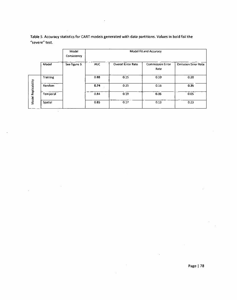
Table 5. Accuracy statistics for CART models generated with data partitions. Values in bold fail the
"severe" test.
Model
Consistency
Model Fit and Accuracy
Model See figure 3. AUC Overall Error Rate Commission Error
Rate
Omission Error Rate
s-Training 0.88 0.15 0.10 0,20
-Q (C U
"5.
Random 0.74 0.25 0.16 0.35
<u cc "5 "D
Temporal 0.84 0.19 0.35 0.05
O 5 Spatial 0.85 0.17 0.13 0.23
Page | 78

Table 6. Summary of how each model performed against the steps in the severe test.
Step 2.
Model Fit and Accuracy
Step 3.
Model
Replicability
Step 4.
Model
Consistency
Step 1. Model
Type
Fit
Training?
Fit
Random?
Fit all other
partitions?
Internally
Consistent?
Fail
severe
test?
Comment
GLM no no no no Yes Best GLM model provides inadequate
predictions with overall error rate of
0.26 and commission error rate of 0.29.
For random partition, commission error
rate also 0.29. Error rates even higher
for other data partitions. Direction of
relationship for CAforest and PR is
inconsistent.
GAM yes no no no Yes Best GAM model fits training data well.
Omission error rates too high for other
data partitions (20.25). CAforest shows
negative relationship for training and
temporal partitions but fairly stable and
near zero relationship for spatial
partition.
CART yes no no somewhat Yes Best CART model fits training partition
well but does not predict other
partitions well, except the spatial
partition. CAforest is the only landscape
predictor that consistently has an above
zero importance value for all partitions.
The split values for CAforest are
consistent across all partitions with
lower amounts of forest increasing the
probability of massasauga occurrence.
Page | 79

Figure 1. Map of the upper Bruce Peninsula region, Ontario. The spatial data partition is shown in blue.
Training, random and temporal data partitions cover areas not shown in blue.
Bruce Peninsula National Park spatial partition
f
Canada
Study Area
USA
Page | 80

Figure 2. GAM model consistency of amount of forest (CAforest) and the likelihood of massasauga
occurrence among data partitions.
Temporal Spatiai Training
| i i [ ii m i i i jiminti«in nii«nt»i^
0.0 0.2 0.4 0.6 0.8 1.0
Caforest
' t p jHimampn^ 0.2 0.4 0.6 0.8 1.0
Caforest
Page | 81

«
Figure 3. Tree model (rpart) showing relationships between selected predictors and the occurrence of
eastern massasauga rattlesnake. Model developed using the training data partition. (X = UTM Easting, Y
= UTM Northing, CAforest = amount for forest, AREAwetland = mean wetland patch size, NPforest =
number of forest patches)
Classification Tree for TRAINING
x>=0.688
105/110
x< C
0 45/7
.2002 —
60/103
() 13/1
y< C .6062 1
47/102
CAforest >=0.6125
—o— 37/27
0 37/14
NPforest
0/13
AREAwetla id>=0.7039
—
10/75
< 0.3891
— 7/15
0 6/2
i 3/60
1/13
Page | 82
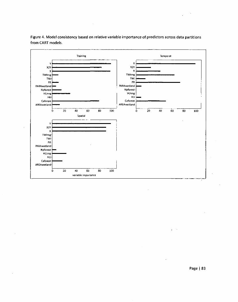
Figure 4. Model consistency based on relative variable importance of predictors across data partitions
from CART models.
Training Temporal
TWIrng Twlrng
TW -
PARAwetland PARAwetland-
Npforest Npforest
HUrng HLlrng
Caforest Caforest-AREAwetland ARtAwetland-
Y-"
X2Y-"
X-
TWIrng-
TWI-
PR-
PARAwetiand-
Npforest"
HUrng*
HLI-
Caforest"
AREAwetland-
0 20 40 60 80
variable importance
100
Page | 83

DISCUSSION
Species distribution models (SDM) and landscape ecology research can offer meaningful
contributions to conservation biology, environmental planning and natural resource protection
strategies because the spatial scales that these activities focus on are consistent with each other (Scott
etal. 2002). Information on species—environment relationships produced by this kind of research can
be used to inform decision making and prioritize conservation options (Primack 2004). However, due to
logistical constraints it is often difficult to replicate such studies. As a consequence, SDMs and other
landscape ecology models are often poorly probed leaving a high potential for spurious results. This may
lead to basing conservation decisions on incorrect information. If this information were more highly
probed conservation decisions could be made with more confidence. Severe tests, as advocated by
Mayo (2004), provides a means to probing potential explanations and reducing to likelihood of spurious
results.
The concept of a severe test in examining hypotheses of models in ecology can be a very useful
means for discriminating between results that could provide the foundation for true explanations in
landscape ecology from results that are spurious. There will always be some kind of spatial pattern in
data used to examine the influence of landscape structure on species distribution and abundance. The
challenge is telling the difference between coincidental spatial patterns in a given data set that give rise
to "significant" results (type 1 statistical errors) from patterns that shed light on an explanation of how
landscape structure affects species. In chapters 1 and 3 of this thesis, if a narrower approach were taken
and results accepted from only one model, conclusions would likely have been very different.
Further effort in the review of the philosophy of science literature and translating this
information into useful tools for landscape ecologists would likely contribute a great deal to the
Page | 84

advancement of landscape ecology. Given the size of areas generally of interest to landscape ecologists
their research often faces significant logistical challenges. Manipulations and controlled experiments are
not generally possible. As a consequence, the discipline often relies on quasi-experiments and
observation studies to study hypotheses. This may lead to a prevalence of spurious results.
Since rigorous controlled experiments are usually not feasible in landscape ecology, researchers
should demand more from the studies they are able to perform. Severe tests are a move in this
direction. Severe tests should involve replicating models across some range of conditions. The specific
conditions will depend on the question and setting of a particular study. Landscape ecologists should
explicitly ask how sensitive their models are to changing patterns in their data and whether these
changes in background conditions are meaningful. If independent data sets represent the same
background conditions but similar models provided inconsistent results then this may be an indicator of
a false model (regardless of how statistically significant it is). Severe tests should also explicitly
incorporate different model types and an assessment of different kinds of model error. Often times the
discovery of how and why models fail can provide for greater understanding than when models succeed.
Severe tests are a conscious effort in trying to make our models fail. If our hypotheses, or models,
continue to pass these severe tests then they deserve a greater degree of support. Landscape ecology
may become a stronger science as a result.
From a conservation biology perspective, independent ground truthing of SDMs should always
be conducted. However, there are times when thorough ground truthing is cost prohibitive or too time
consuming to be relevant for a particular land use decision. In these instances, severe tests that more
highly probe SDMs may provide some insight as to whether certain models should be used for
conservation planning. Severe tests should not be viewed as a surrogate for ground truthing but rather
as a tool to gain support and confidence for a set of models. Severe tests may be useful in ranking a set
Page | 85

of models where only the most successful models are selected for independent ground truthing in order
to minimize costs. In this sense, severe tests of SDMs may be a precursor to ground truthing.
There is no single severe test that one should conduct for evaluating SDMs. A specific severe
test will be specific to the goals and objectives of the planning context that the SDM is to inform. Most
severe tests should involve some kind of assessment of SDMs with independent data. It is
recommended that SDMs be evaluated with, at least, one or more random partitions of the original
data. However, these random partitions represent that same spatio-temporal context as the original
training data and, therefore, do not completely represent an independent assessment. For this reason, a
severe test of a SDM should involve, where possible, comparisons with spatio-temporal independent
data that represent similar but different contexts.
The notion of a severe test is a flexible one and merely relates to strategies that attempt to
probe hypotheses or models more deeply than simple null hypothesis statistical tests. A severe test is
part of an overall research strategy. There are instances where studies in conservation biology are
rigorously designed and implemented that provide unequivocal results. In these instances, severe tests
may not be necessary. However, this is generally not the case for SDMs as these models are essentially
data mining tools that relate patterns of available species occurrence records with patterns in
environmental variables (Scott etal. 2002).
Generally speaking, for conservation planning, the importance of severe tests should be reflective of the
ability to undertake a rigorous study design. Information garnered through controlled studies with
sufficient replication can be more directly applied to decision making. Information gathered through
observational studies, quasi-experiments, or data mining should be viewed with greater suspicion by
Page | 86

decision makers. In these cases, severe tests take on an increased importance. Essentially, the notion of
a severe test becomes increasingly important as the rigour of studjes decrease.
Page | 87

REFERENCES
Achinstein, P. 2001. The Book of Evidence. Oxford University Press, New York, NY.
Achinstein, P. 2005. Scientific Evidence: Philosophical Theories and Applications. John Hopkins University
Press, London, U.K.
Allen T.F.H. and T.W. Hoekstra 1992. Toward a Unified Ecology. Columbia University Press, New York,
NY.
Austin, M.P. 2002. Spatial prediction of species distribution: an interface between ecological theory and
statistical modelling. Ecological Modelling. 157:101-118.
Betts, M.G., Forbes, G.J., Diamond, A.W. and P.D. Taylor. 2006. Independent effects of fragmentation on
forest songbirds: an organism-based approach. Ecological Applications 16:1076-1089
Betts, M.G., Hagar, J.C., Rivers, J.W., Alexander, J.D., McGarigal, K. and B.C. McComb. 2010. Thresholds
in forest bird occurrence as a function of the amount of early-seral broadleaf forest at landscape scales.
Ecological Applications 20: 2116-2130.
Borcard, D. and P. Legendre. 2002. All-scale spatial analysis of ecological data by means of principal
coordinates of neighbour matrices. Ecological Modelling 153: 51-68.
Breiman, L. 2010. randomForest: Breiman and cutler's random forests for classification and regression.
http://cran.r-Droiect.ore/web/packages/randomForest/index.html.
Breiman, L., Friedman, J. H., Olshen, R. A. and C.J. Stone. 1984. Classification and Regression Trees.
Wadsworth & Brooks, Monterey, CA.
Page | 88
Brennan, J., Bender, D.J., Contreras, T.A. and L. Fahrig. 2002. Focal patch landscape studies for wildlife
management: optimizing sampling effort across scales. Pages 68-91 in J. Liu and W. W. Taylor, editors.
Integrating Landscape Ecology into Natural Resource Management. Cambridge University Press,
Cambridge, MA.
Brubaker, P. H. 2008. Study Design and analysis: Do Not Be Statistically Cenophobic: Time to ROC and
Roll! Journal of Cardiopulmonary Rehabilitation and Prevention 28:420-421.
Burnham, K.P. and D.R. Anderson. 2002. Model Selection and Inference: A Practical Information-
Theoretic Approach, 2nd e.d. Springer-Verlag, New York, N.Y.
Carmel, Y. 2004. Controlling data uncertainty via aggregation in remotely sensed data. IEEE Geoscience
and Remote Sensing Letters 1: 39-41.
Conant, R. and J.T. Collins. 1991. A Field Guide to Reptiles and Amphibians: Eastern and Central North
America, 3rd e.d. Houghton Mifflin Company, New York, NY.
Culp, M., Johnson, K. and G. Michailidis. 2010. ada: an R package for stochastic boosting, http://cran.r-
proiect.org/web/packaees/ada/index.html.
Davis, R. H. 2006. Strong Inference: rationale or inspiration? Perspectives in Biology and Medicine 49:
238-250.
Desrochers, A., Renaud, C., Hochachka, W.M. and M. Cadman. 2010. Area-sensitivity by forest
songbirds: theoretical and practical implications of scale-dependency. Ecography 33: 921-931.
Dimitriadou, E. 2011. el071: Misc Functions of the Department of Statistics (el071). http://cran.r-
proiect.org/web/packages/el071/index.html.
Page | 89

Dobson, A.J. and A.G. Barnett. 2008. Introduction to Generalized Linear Models, 3rd e.d. Chapman and
Hall/CRC Press, Boca Raton, FL.
Dunford, W. and K. Freemark. 2004. Matrix matters: effects of surrounding land uses on forest birds
near Ottawa, Canada. Landscape Ecology 20:497-511.
Eastern Massasauga Rattlesnake Recovery Team. 2005. Guidelines for identifying significant portions of
the habitat, and significant wildlife habitat, for the eastern massasauga rattlesnake in eastern Georgian
Bay And Bruce Peninsula populations, Ontario. Version 1.0. 20pp.
Eigenbrod, F., Hecnar, SJ. and L. Fahrig. 2011. Sub-optimal study design has major impacts on
landscape-scale inference. Biological Conservation 144: 298-305.
Elith, J., Graham, C. H., Anderson, R. P., Dudi'k, M., Ferrier, S., Guisan, A., Hijmans, R. J., Huettmann, F.,
Leathwick, J. R., Lehmann, A., Li, J., Lohmann, L. G., Loiselle, B. A., Manion, G., Moritz, C., Nakamura, M.,
Nakazawa, Y., Overton, J. McC., Peterson, A. T., Phillips, S. J., Richardson, K. S., Scachetti-Pereira, R.,
Schapire, R. E., Sobero'n, J., Williams, S., Wisz, M. S. and N.E. Zimmermann. 2006. Novel methods
improve prediction of species' distributions from occurrence data. Ecography. 29:129-151.
Elith J. and J.R. Leathwick. 2009. Conservation prioritization using species distribution models. Pages 70-
93 in A. Moilanen, K.A. Wilson, H.P. Possingham, (eds.). Spatial Conservation Prioritization: Quantitative
Methods and Computational Tools. Oxford University Press, London, U.K.
Elith, J., Kearney, M. and S. Phillips. 2010. The art of modelling range-shifting species. Methods in
Ecology and Evolution 1:330-342.
Page | 90
Engler, R., Guisan, A. and L. Rechsteiner, 2004. An improved approach for predicting the distribution of
rare and endangered species from occurrence and pseudo-absence data. Journal of Applied Ecology 41:
263-274.
ESRI 2011. ArcGIS Desktop: Release 10. Environmental Systems Research Institute, Redlands, CA.
Ewers, R.M. and R.K. Didham. 2006. Confounding factors in the detection of species responses to
habitat fragmentation. Biological Reviews 81:117-142.
Ethier, K. and L. Fahrig. 2011. Positive effects of forest fragmentation, independent of forest amount on
bat abundance in eastern Ontario, Canada. Landscape Ecology 26: 865-876.
Fahrig, L. 1998. When does fragmentation of breeding habitat affect population survival? Ecological
Modelling 105: 273-292.
Fahrig, L. 2001. How much habitat is enough? Biological Conservation 100: 65-74.
Fahrig, L. 2003. Effects of habitat fragmentation on biodiversity. Annual Review of Ecology and
Systematics 34:487-515.
Fahrig L. 2005. When is a landscape perspective important? Pages 3-10 in J.A. Wiens, M.R. Moss, editors.
Issues and perspectives in landscape ecology. Cambridge University Press, Cambridge, U.K.
Fielding, A.H. and J.F. Bell. 1997. A review of methods for the assessment of prediction errors in
conservation presence/ absence models. Environmental Conservation 24: 38-49.
Franklin, J. 2009. Mapping Species Distributions: Spatial Inference and Prediction. Cambridge University
Press. Cambridge, U.K.
Government of Canada. 2002. Species at Risk Act, SC 2002, c 29, http://canlii.ca/t/ld71. Ottawa, ON.
Page | 91

Guisan, A. and N.E. Zimmermann. 2000. Predictive habitat distribution models in ecology. Ecological
Modelling 135:147-186.
Guisan, A. and W. Thuiller. 2005. Predicting species distribution: offering more than simple habitat
models. Ecology Letters 8: 993-1009.
Hanski, I. 1999. Metapopulation Ecology. Oxford University Press, New York, NY.
Harris, L.D. 1988. Edge effects and conservation of biotic diversity. Conservation Biology. 2:330-332.
Hastie, T.J. and R.J. Tibshirani. 1991. Generalized additive models. Chapman & Hall/CRC Press, New
York, NY.
Hastie, T., Tibshirani, R. and J.H. Friedman. 2001. The Elements of Statistical Learning: Data Mining,
Inference, and Prediction. Springer-Verlag, New York, NY.
Heglund, P.J. 2002. Foundations of species-environment relations. Pages 35-41 in J. M. Scott, P.J.
Heglund, M.L. Morrison, editors. Predicting species occurrences: issues of scale and accuracy. Island
Press, Washington, DC.
Hempel, C. 1965. Aspects of scientific explanation. Free Press, New York, N.Y.
Hilborn, R. and S.C. Stearns. 1982. On inference in ecology and evolutionary biology: the problem of
multiple causes. Acta Biotheoretica 31:145-164.
Hijmans, R.J. and J. van Etten. 2011. Package 'raster'. Geographic analysis and modeling with raster
data. http://raster.r-forge.r-proiect.org/.
Page | 92

Hinam, H.L. and C.C. St. Clair. 2008. High levels of habitat loss and fragmentation limit reproductive
success by reducing home range size and provisioning rates of northern saw-whet owls. Biological
Conservation 141: 524-535.
Houlahan, J. and C.S. Findlay. 2003. The effects of adjacent land use on wetland amphibian species
richness and community composition. Canadian Journal of Fisheries and Aquatic Sciences 60:1078-
1094.
Huston, M.A. 2002. Introductory essay: critical issues for improving predictions. Pages 7-21 in J. M.
Scott, P.J. Heglund, M.L. Morrison, editors. Predicting Species Occurrences: Issues of Scale and
Accuracy. Island Press, Washington, DC.
Johnson, D.H. 1999. The insignificance of statistical significance testing. The Journal of Wildlife
Management. 63(3): 763-772.
Johnson, G., Parent, C., Kingsbury, B., Seigel, R., King, R. and J. Szymanski. 2000. The eastern massasauga
rattlesnake: a handbook for land managers. US Fish and Wildlife Service, Fort Snelling, MN.
http://midwest.fws.gov/Endangered/reptiles/eama-mgmt-euide.pdf.
Keitt, T.H., Bivand, R., Pebesma, E. and B. Rowlingson. 2011. rgdal: Bindings for the Geospatial Data
Abstraction Library, http://cran.r-proiect.org/web/packages/rgdal/index.html.
Koper, N. and F.K.A. Schmiegelow. 2006. A multi-scaled analysis of avian response to habitat amount
and fragmentation in the Canadian dry mixed-grass prairie. Landscape Ecology 21:1045-1059.
Krawchuk, M. A. and P.D. Taylor. 2003. Changing importance of habitat structure across multiple spatial
scales for three species of insects. Oikos 103:153-161.
Page | 93

Kuhn, M. 2011. caret: Classification and Regression Training, http://cran.r-
proiect.org/web/Dackages/caret/index.html
Lawler, J.J., Wiersma Y.F. and F. Huettmann. 2011. Using species distribution models for conservation
planning and ecological forecasting. In. C.A. Drew et at. (eds). Predictive Species and Habitat Modeling in
Landscape Ecology: Concepts and Applications. Springer. New York, N.Y.
Lampila, P., Monkkonen, M. and A. Desrochers. 2005. Demographic responses by birds to forest
fragmentation. Conservation Biology 19:1537-1546.
Lindenmayer, D.B. and J. Fischer. 2006. Tackling the habitat fragmentation panchreston. Trends in
Ecology and Evolution 22:127-132.
Liu, C., White, M. and G. Newell. 2011. Measuring and comparing the accuracy of species distribution
models with presence-absence data. Ecography 34: 232-243.
Lobo, J. M., Jimenez-Valverde, A. and R. Real. 2008. AUC: a misleading measure of the performance of
predictive distribution models. Global Ecology and Biogeography 17:145-151.
Lobo, J.M., Jimenez-Valverde, A. and J. Hortal. 2010. The uncertain nature of absences and their
importance in species distribution modelling. Ecography 33:103-114.
Luck, G.W. 2003. Differences in the reproductive success and survival of the rufous treecreeper
{Climactius rufa) between a fragmented and unfragmented landscape. Biological Conservation 109:1-
14.
Mackie, J.L. 1965. Causes and conditions. American Philosophical Quarterly 2: 245-264.
Page | 94

MacLeod, C. D., Madleberg, L., Schweder, C., Bannon, S. and M. Pierce. 2008. A comparison of
approaches for modelling the occurrence of marine animals. Hydrobiologia 612: 21-32.
Mayo, D. G. 1991. Novel evidence and severe tests. Philosophy of Science 58: 523-552.
Mayo, D. G. 2004. Evidence as passing severe tests: highly probed vs. highly proved. Pages 95-127 in P.
Achinstein, editor. Scientific Evidence. Johns Hopkins University Press, Baltimore, MD.
Mayo, D.G. and A. Spanos. 2006. Severe testing as a basic concept in a Neyman-Pearson philosophy of
induction. The British Journal for the Philosophy of Science 57: 323-357.
McCullagh, P. and J. Nelder. 1989. Generalized Linear Models. Second Edition. Chapman and Hall/CRC.
Boca Raton, FL.
McCullough, D.R. and R.H. Barrett, (eds.). Wildlife 2001: Populations. Elsevier Applied Science. London,
U.K.
McGarigal, K., Cushman, S.A., Neel, M.C. and E. Ene. 2002. FRAGSTATS: Spatial Pattern Analysis Program
for Categorical Maps. University of Massachusetts, Amherst, MA.
Metz, C.E. 1978. Basic principles of ROC analysis. Seminars in Nuclear Medicine 8: 283-298.
Milborrow, S. 2011. earth: multivariate adaptive regression spline models, http://cran.r-
proiect.org/web/packages/earth/index.html.
O'Brien, R. 2007. A caution regarding rules of thumb for variance inflation factors. Quality and Quantity
41: 673-690.
Page | 95

O'Connor, R.J., 2002. The conceptual basis of species distribution modelling; time for paradigm shift.
Pages 25-33 in J. M. Scott, P.J. Heglund, M.L. Morrison, editors. Predicting Species Occurrences: Issues
of Scale and Accuracy. Island Press, Washington, DC.
Oksanen, J., Blanchet, F. G., Kindt, R., Legendre, P., O'Hara, R. B., Simpson, G. L., Solymos, P., Henry, M.,
Stevens, H. and H. Wagner. 2010. Package Vegan. Community Ecology Package.
Oksanen, L. 2001. Logic of experiments in ecology: is pseudoreplication a pseudoissue? Oikos 94: 27-38.
Parent, C. and P.J. Weatherhead. 2000. Behavioural and life history responses of eastern massasauga
rattlesnakes (Sistrurus catenatus catenatus) to human disturbance. Oecologia 125:170-178.
Parks Canada. 2005. Bruce Peninsula National Park: State of the Park Report. Government of Canada,
Gatineau, QC.
Pearce, J.L. and S. Ferrier. 2000. Evaluating the predictive performance of habitat models developed
using logistic regression. Ecological Modelling 133: 225-245.
Pearce, J.L., Vernier, L.A., Ferrier, S. and D.W. McKenney. 2002. Measuring prediction uncertainty in
models of species distribution. Pages 383-390 in J. M. Scott, P.J. Heglund, M.L. Morrison, (eds.).
Predicting Species Occurrences: Issues of Scale and Accuracy. Island Press, Washington, DC.
Phillips, S. J., Dudfk, M. and R.E. Schapire. 2004. A maximum entropy approach to species distribution
modeling. Pages 655-662 in Proceedings of the Twenty-First International Conference on Machine
Learning.
Phillips, S.J., Anderson, R.P. and R.E. Schapire. 2006. Maximum entropy modeling of species geographic
distributions. Ecological Modelling 190:231-25.
Page | 96

Pickett, S.T.A., Kolasa, J. and C.G. Jones. 1994. Ecological Understanding: The Nature of Theory and the
Theory of Nature. Academic Press, San Diego, CA.
Piatt, J. R. 1964. Strong inference. Science 146: 347-353.
Popper, K. R. 1934. The Logic of Scientific Discovery. Hutchinson, London, UK.
Primack, Richard B. 2004. A Primer of Conservation Biology. 3rd ed. Sinauer Associates. Sunderland,
Mass.
Prior, K.A. and P.J. Weatherhead. 1994. Response of free-ranging eastern massasauga rattlesnake to
human disturbance. Journal of Herpetology 28: 255-257.
Prior, K. 1999. Recovery priorities for the eastern massasauga. Pages 28-30 in B. Johnson and M. Wright,
editors. Second International Symposium and Workshop on the Conservation of the Eastern
Massasauga Rattlesnake, Sistrurus catenatus catenatus: population and habitat management issues in
urban, bog, prairie and forested ecosystems. Toronto Zoo, Toronto, ON.
Quinn, J.F. and A.E. Dunham. 1983. On hypothesis testing in ecology and evolution. The American
Naturalist 122: 602-617.
Raerinne, J. 2010. Causal and mechanistic explanation in ecology. Acta Biotheoretica 59: 251-271.
Radford, J.Q., Bennett, A.F., and G J. Cheers. 2005. Landscape-level thresholds of habitat cover for
woodland-dependent birds. Biological Conservation 124: 317-337.
Ripley, B. 2009. nnet: Feed-forward Neural Networks and Multinomial Log-Linear Models, http://cran.r-
proiect.org/web/packaees/nnet/index.html.
Page | 97

Ritchie, L.E., Betts, M.G., Forbes, G., and K. Vernes. 2009. Effects of landscape composition and
configuration on northern flying squirrels in a forest mosaic. Forest Ecology and Management. 257:
1920-1929.
Rizkalla, C.E. and R.K. Swihart. 2006. Community structure and differential responses of aquatic turtles
to agriculturally induced habitat fragmentation. Landscape Ecology 21:1361-1375.
Robinson, S.K., Thompson III, F.R., Donovan, T.M., Whitehead, D.R. and J. Faaborg. 1995. Regional
forest fragmentation and the nesting success of migratory birds. Science 267:1987-1989.
Rosenberg, M.S. and C.D. Anderson. 2011. PASSaGE: Pattern Analysis, Spatial Statistics and Geographic
Exegesis. Version 2. Methods in Ecology and Evolution 2: 229-232.
Rouse, J.D. and R.J. Wilson. 2001. Update COSEWIC Status Report on the Eastern Massasauga, Sistrurus
catenatus catenatus. Prepared for the Committee of the Status of Endangered Wildlife in Canada
(COSEWIC), November 2001.
Rytwinski, T. and L. Fahrig. 2011. Reproductive rate and body size predict road impacts on mammal
abundance. Ecological Applications 21: 589-600.
Salmon, W. C. 1998. Causality and Explanation. Oxford University Press, New York, NY.
Schlossberg, S. and D.I. King. 2009. Post-logging succession and habitat usage of shrubland birds. Journal
of Wildlife Management 73: 226-231.
Scott, J.M., Heglund, P.J., Haufler, J.B., Morrison, M., Raphael, M.G., and W.B. Wall. (eds.). 2002.
Predicting Species Occurrences: Issues of Accuracy and Scale. Island Press, Covelo, CA.
Page | 98

Sing, T. 2009. ROCR: Visualizing the performance of scoring classifiers, http://cran.r-
proiect.org/web/packaees/ROCR/index.html.
Smith, A.C., Koper, N., Francis, C.M., and L. Fahrig. 2009. Confronting collinearity: comparing methods
for disentangling the effects of habitat loss and fragmentation. Landscape Ecology 24:1271-1285.
Smith, A.C., Fahrig, L., and C.M. Francis. 2011. Landscape size affects the relative importance of habitat
amount, habitat fragmentation, and matrix quality on forest birds. Ecography34:103-113.
Sober, E. 1988. Apportioning causal responsibility. The Journal of Philosophy 85: 303-318.
Therneau, T.M., Atkinson, B., and B. Ripley. 2011. rpart: Recursive Partitioning, http://cran.r-
proiect.org/web/packages/rpart/index.html.
Trzcinski, M.K., Fahrig, L., and G. Merriam. 1999. Independent effects of forest cover and fragmentation
on the distribution of forest breeding birds. Ecological Applications 9: 586-593.
VanDerWal, J., Shoo, L.P., Graham, C., and S.E. Williams. 2009. Selecting pseudo-absence data for
presence only distribution modeling: how far should you stray from what you know? Ecological
Modelling 220: 589-594.
Verner, J., Morrison, M.L., and C.J. Ralph. 1986. Wildlife 2000: Modelling Habitat Relationships of
Terrestrial Vertebrates. University of Wisconsin Press, Madison, Wl.
Villard, M.-A., Trzcinski, M.K., and G. Merriam. 1999. Fragmentation effects on forest birds: relative
influence of woodland cover and configuration on landscape occupancy. Conservation Biology 13: 774-
783.
Page | 99

Wang, G., Gertner, G. Z., Fang, S., and A.B. Anderson. 2005. A methodology for spatial uncertainty
analysis of remote sensing and GIS products. Photogrammetric Engineering and Remote Sensing 71:
1423-1432.
Warren, T.L., Betts, M.G., Diamond, A.W., and G.J. Forbes. 2005. The influence of local habitat and
landscape composition on cavity-nesting birds in a forested mosaic. Forest Ecology and Management
214: 331-343.
Weatherhead, P.J. and K.A. Prior. 1992. Preliminary observations of habitat use and movements of the
eastern massasauga rattlesnake (Sistrurus c. catenatus). Journal of Herpetology 26:447-452.
Wood, S. 2011. mgcv: GAMs with GCV/AIC/REML smoothness estimation and GAMMs by PQL.
http://cran.r-proiect.org/web/packages/mecv/index.html.
Woodward, J. 2003. Making Things Happen: A Theory of Causal Explanation. Oxford University Press,
Oxford, UK.
Woodward, J. 2010 Causation in biology: stability, specificity, and the choice of levels of explanation.
Biology and Philosophy 25: 287-318.
Ylikoski P. and J. Kuorikoski. 2010. Dissecting explanatory power. Philosophical Studies 148: 201-219.
Zharikov, Y., Elner, R.W., Shepherd, P.C.F., and D.B. Lank. 2009. Interplay between physical and
predator landscapes affects transferability of shorebird distribution models. Landscape Ecology 24:
129-144.
Zitske, B.P., Betts, M.G, and A.W. Diamond. 2011. Negative effects of habitat loss on survival of migrant
warbiers in a forest mosaic. Conservation Biology 25: 993-1001.
Page | 100

Zuur, A. F., Leno, E.N., and G.M. Smith. 2007. Analysing Ecological Data: Statistics for Biology and Health.
Springer, New York, NY.
Page | 101
Top Related