


Languages
Pages
Legal


1
1
Determining the effects of multimodal grain size distribution on the hydraulic conductivity
of glacial outwash sediments, Selden, Long Island, NY
A Final Project presented
By
Roselina Quadros
In Partial Fulfillment of the
Requirements for the Degree of
“Master of Science
In
Geosciences with concentration in Hydrogeology”
Stony Brook University
December, 2015

2
2
We, the final report committee for the above candidate for the Master of Science degree,
hereby recommend
Acceptance of this report.
Dr. Gilbert Hanson
Professor of Geosciences
Research Advisor
Dr. Martin A. Schoonen
Professor of Geochemistry
Dr. Henry Bokuniewicz
Professor of Marine Science
School of Marine and Atmospheric Sciences
3
3
Abstract
The grain-size distribution in the Upper Glacial aquifer on Long Island is dominantly multimodal with angular and low sphericity grains. The purpose of this study was to determine if grain-size distribution, shape and angularity of the sediments affect the hydraulic conductivity calculated using empirical grain-size analysis methods. Upper Glacial aquifer sediments were collected on the Suffolk County Community College Campus in Selden, NY using direct push cores. These sediments were analyzed for grain-size, shape and angularity.
Hydraulic conductivity was determined by grain-size distribution based on sieve analysis for grain-sizes greater than 1mm and by laser diffractometry (MasterSizer) for grain-sizes less than 1mm. Five methods (Kozeny-Carman, Hazen, Breyer, Slitcher and Terzaghi), were used to determine the hydraulic conductivities of unimodal and multimodal sediments . The hydraulic conductivity values range from 0.13 ft/d for gravelly muddy sand to 411 ft/d for a unimodal, moderately sorted sandy gravel. When the empirical formulas for unimodal sediments were used on multimodal sediments to determine hydraulic conductivity; Breyer, Kozeny –Carman and Hazen method were found highly effective based on distribution and sediment type. Using these equations intended for unimodal sediments do lead to significant errors if used on multimodal sediments. The actual conductivities may be greater or less than the calculated conductivities depending on the location and nature of the modes.

4
4
Table of Contents
List of Figures: .................................................................................................................................. 5
List of Tables: ........................................................................................................................... 8
Acknowledgements:................................................................................................................. 9
Introduction: .................................................................................................................................. 10
Section 1: Geology of the Study Area ............................................................................................ 12
Section 2: Methods ........................................................................................................................ 14
Section 2.1: Sample Selection-Selden -Long Island: .................................................................. 14
Section 2.1 a: Core Logging .................................................................................................... 14
Section 2.2 Grain-size distribution analysis-Standard sieving method: ..................................... 14
Section 2.3: High-Resolution Grain-size through Laser Diffractometry .................................... 14
Sample Preparation ............................................................................................................... 15
Section 2.4: Application of Gradistat 4.0 software program (statistical analysis) in obtaining
the data to determine the hydraulic conductivity parameters for calculations..................................... 15
Section 2.5: Determining the hydraulic conductivity using empirical formulas from grain-
size distribution analysis. .................................................................................................................... 16
Section 2.6: Grain shape analysis using the microscope ........................................................... 18
Section 3: Results ....................................................................................................................... 21
Section 3.1: grain-size sieve analysis, MasterSizer Results ........................................................ 23
Section 3.2: Gradistat grain-size analysis results ................................................................... 25
Section 3.3: Shape and Angularity results from the microscopic experiment .......................... 31
Section 3.4: Hydraulic conductivity for samples with unimodal grain-size distributions. ......... 34
................................................................................................................................................... 35
Section 3.5: Comparison of the multimodal and unimodal distribution conductivity results ... 37
....................................................................................................................................................... 44
Section 3.6: Variations in hydraulic conductivity using different empirical methods .......... 45
....................................................................................................................................................... 45
Section 4: Discussion: .................................................................................................................... 51
Conclusion: ........................................................................................ Error! Bookmark not defined.
References Cited ........................................................................................................................ 52

5
5
List of Figures:
Figure 1: Map of Long Island. The arrow points to the sampling site on the Selden campus of Suffolk County
Community College (Microsoft Corp. 2003). ................................................................................................ 12
Figure 2: The location of the site (arrow) is indicated just south of the baseball fields on this map of the Selden
campus of Suffolk County Community College (Google Earth) ..................................................................... 13
Figure 3: Geologic cross section of Long Island (Delaguna, 1963) ......................................................................... 13
Figure 4: Sediment pictures of RQ-1 (pebbly Loess), RQ-12 (sand) and RQ 21 (Muddy Sandy Gravel) examined
under the petrographic microscope to determine angularity and sphericity. .............................................. 19
Figure 5: Sediment pictures of Sample RQ-3 (Gravelly Muddy Sand) and RQ-8 (Gravelly sand) grains examined
under the petrographic microscope to determine angularity and sphericity. .............................................. 20
Figure 5a: Picture shows specimen set-up and Sample specimen of the grains observed under the petrographic
microscope with a magnification of 31.5 (2.5 objective and 12.5x ocular to determine angularity and
sphericity ..................................................................................................................................................... 20
Figure 6: Powers scale of roundness and sphericity chart. ................................................................................... 21
Figure 7: Sedimentary log of core from Upper Glacial aquifer sediments on Suffolk Community College campus.
.................................................................................................................................................................... 22
Figure 8: RQ-1 with bimodal grain-size distribution for pebbly loess at 2.3 feet depth. ....................................... 23
Figure 9: RQ-3 grain-size distribution for coarse sand and gravel at 4 feet below surface. ................................... 23
Figure 10: RQ-16 grain-size distribution curve for unimodal fine to-medium grain sand at 22.6 feet below surface.
.................................................................................................................................................................... 23
Figure 11: RQ-21 sandy gravel grain-size distribution curve for bimodal distribution for a Muddy sandy gravel at
36 ft .below surface; the bottom of the core. .............................................................................................. 24
Figure 12: Grain-size distribution curves generated by the laser diffractometry for all 21 samples (RQ-1 to RQ-
21). .............................................................................................................................................................. 24
24
Figure 13: Gradistat indicating that the skewness and sorting is not reliable for the following sample-RQ-
1(pebbly Loess) due to sample being multimodal ........................................................................................ 25
Figure 14: Gradistat – grain-size distribution graph of sample RQ-1 (Pebbly Loess) indicating a polymodal
distribution for mixed bins data and trimodal for half phi graph. ................................................................ 26
Figure 15: Gradistat –grain-size distribution graph for sample RQ-3(muddy sandy gravel) indicating a multimodal
distribution from the sieves and MasterSizer data combined and half phi. ................................................. 28
Figure 16: Gradistat –grain-size distribution graph for poor sorted sample RQ-8 (Sand)) indicating a bimodal
distribution from the sieves and MasterSizer (mixed-bin) and half phi data................................................ 30
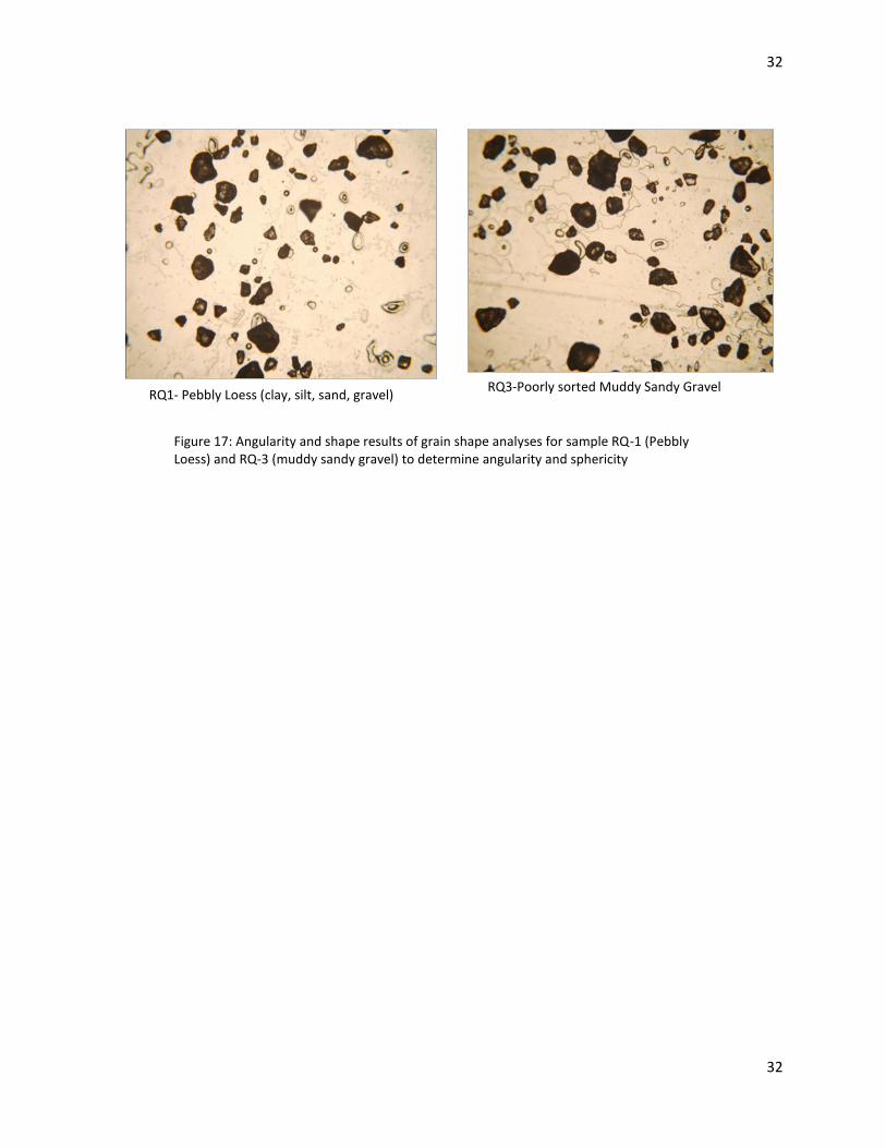
RQ1- Pebbly Loess (clay, silt, sand, gravel) ........................................................................................................... 32
RQ3-Poorly sorted Muddy Sandy Gravel .............................................................................................................. 32
Figure 17: Angularity and shape results of grain shape analyses for sample RQ-1 (Pebbly Loess) and RQ-3 (muddy
sandy gravel) to determine angularity and sphericity .................................................................................. 32
Figure 19: sample RQ-1 (polymodal-Pebbly Loess) Results- depicting the unimodal and multimodal distribution
difference. ................................................................................................................................................... 40
Figure 20: Sample RQ-3 (Muddy sandy gravel) depicting the difference in unimodal and multimodal parameters
to calculate the hydraulic conductivity. ....................................................................................................... 41
Figure 21: sample RQ-8 (Gravelly sand) results depicting the percentage difference between the unimodal and
multimodal distribution in determining the hydraulic conductivity. .......................................................... 42

6
6
Figure 22: RQ-19 (Sandy Gravel at 32 feet below ground sample results showing the conductivity difference
between the unimodal and multimodal distribution ................................................................................... 43
Figure 23: RQ-21 (Muddy Sandy Gravel at 36feet below ground) sample results showing the Conductivity
difference between the unimodal and multimodal distribution .................................................................. 44
Figure 24: shows a plot of temperature vs. g/v –As temperature increases g/v value increases ......................... 45
Figure 25: shows a plot of U vs. f(n) for Hazen's method .................................................................................... 45
Figure 27: shows a plot of U vs. f(n) for Breyer Method ..................................................................................... 46
Figure 26: shows a plot of U vs. f(n) for Kozeny-Carman method ....................................................................... 46
Figure 28: shows a plot of U vs. f(n) for Terzaghi Method .................................................................................. 47
Figure 29: U vs. K value for unimodal (figured out by plotting U vs. f(n)) ............................................................. 47
Figure 30: U vs. K value for multimodal (figured out by plotting U vs. f(n)) .......................................................... 48
Figure 31: d10 vs. K value for unimodal sediments showing a direct relationship between the d10 and K. As d10
increases K increases. .................................................................................................................................. 48
Figure 32: d10 vs. K value for multimodal sediments showing a direct relationship between d10 and K. As d10
increases conductivity increases. ................................................................................................................. 49
Figure 33: As d10^2 increases, f(n) value decreases; which would also change the conductivity value by same
percent ........................................................................................................................................................ 50
Figure 34: Mastersizer Results; particle size distribution curves for sample (RQ-2, RQ-3, RQ-4, RQ-5, RQ-6, RQ-7,
RQ-8, and RQ-9)........................................................................................................................................... 53
Figure 35: Mastersizer Results; particle size distribution curves for sample (RQ-10, RQ-11, RQ-12, RQ-13, RQ 14,
and RQ-15) .................................................................................................................................................. 53
Figure 36: Mastersizer Results; particle size distribution curves for sample (RQ-17, RQ-18, RQ-19, and RQ-20) .. 53
Figure 37: mixed bin grain size distribution for samples RQ-1 and RQ 2 indicating Polymodal and Bimodal
distribution ................................................................................................................................................. 53
Figure 38: mixed bin grain size distribution for samples RQ-3 and RQ 4 indicating Bimodal and Unimodal
distribution ................................................................................................................................................. 53
Figure 39: mixed bin grain size distribution for samples RQ-5 and RQ 6 indicating Unimodal and Unimodal
distribution ................................................................................................................................................. 53
Figure 40: mixed bin grain size distribution for samples RQ-7 and RQ 8 indicating Unimodal and Bimodal
distribution ................................................................................................................................................. 53
Figure 41: mixed bin grain size distribution for Gravelly sand (RQ-9) indicating Unimodal distribution ............... 53
Figure43: mixed bin grain size distribution for sand (RQ-10) and gravelly sand (RQ11) indicating Unimodal and
Unimodal distribution ................................................................................................................................. 53
Figure 42: mixed bin grain size distribution for samples RQ-12 and RQ 13 indicating Unimodal and Unimodal
distribution ................................................................................................................................................. 53
Figure 44: mixed bin grain size distribution forRQ-14 (Gravelly sand) indicating Unimodal distribution .............. 53
Figure 45: mixed bin grain size distribution for sand (RQ-16) and gravelly sand (RQ 17) indicating Unimodal
distribution ................................................................................................................................................. 53
Figure 46: mixed bin grain size distribution for sand (RQ-18) and sandy gravel (RQ 19) indicating unimodal and
Trimodal distribution................................................................................................................................... 53
Figure 47: Microscopic images of the grains (grain shape analysis) - Showing the shape and angularity of the
grains for sample RQ1sample RQ-21 ........................................................................................................... 53
Sample RQ-21: Grain shape results ...................................................................................................................... 53
Figure 48: Grain size distribution –Half phi-Sample RQ-1(polymodal) to RQ-2 (bimodal) indicating a change in
resolution hence varying modes. ................................................................................................................. 53

7
7
Figure 49: Grain size distribution –Half phi-Sample RQ-3(Bimodal) to RQ-4 (unimodal) indicating a change in
resolution hence varying modes. ................................................................................................................. 53
Figure 50: Grain size distribution –Half phi-Sample RQ-5(Unimodal) to RQ-6 (unimodal) indicating a change in
resolution hence varying modes. ................................................................................................................. 53
Figure 51: Grain size distribution –Half phi-Sample RQ-7(Unimodal) to RQ-8 (Bimodal) indicating a change in
resolution hence varying modes. ................................................................................................................. 53
Figure53: Grain size distribution –Half phi-Sample RQ-11 (Unimodal) to RQ-12 (Unimodal) indicating a change in
resolution hence varying modes. ................................................................................................................. 53
Figure 52: Grain size distribution –Half phi-Sample RQ-9 (Unimodal) to RQ-10 (Unimodal) indicating a change in
resolution hence varying modes. ................................................................................................................. 53
Figure 54: Grain size distribution –Half phi-Sample RQ-13 (Unimodal) to RQ-14 (Unimodal) indicating a change in
resolution hence varying modes. ................................................................................................................. 53
Figure 55: Grain size distribution –Half phi-Sample RQ-15 (Unimodal) to RQ-16 (Unimodal) indicating a change in
resolution hence varying modes. ................................................................................................................. 53
Figure 56: Grain size distribution –Half phi-Sample RQ-17 (Unimodal) to RQ-18 (Unimodal) indicating a change in
resolution hence varying modes. ................................................................................................................. 53
Figure 57: Grain size distribution –Half phi-Sample RQ-19 (Trimodal) to RQ-20 (Bimodal) indicating a change in
resolution hence varying modes. ................................................................................................................. 53
Figure 58: Grain size distribution –Half phi-Sample RQ-21 (Bimodal) indicating a change in resolution hence
varying modes. ............................................................................................................................................ 53
Figure 59: Samples pictures of RQ-1(polymodal loess), RQ 2(bimodal loess), RQ-3(Bimodal gravelly sand) grains
examined under the petrographic microscope to determine the angularity and sphericity. ........................ 53
Figure 60: Samples pictures of RQ-4(Unimodal gravelly sand .............................................................................. 53
) to RQ5 (Unimodal sand) grains examined under the petrographic microscope to determine the angularity and
sphericity..................................................................................................................................................... 53
Figure 61: Samples pictures of RQ-6 (Unimodal gravelly sand) to RQ-7(Unimodal gravelly sand) grains examined
under the petrographic microscope to determine the angularity and sphericity. ........................................ 53
Figure 63: Samples pictures of RQ-10 (Unimodal sand) to RQ-11(Unimodal gravelly sand) grains examined under
the petrographic microscope to determine the angularity and sphericity. .................................................. 53
Figure 62: Samples pictures of RQ-8 (bimodal gravelly sand) to RQ-9 (Unimodal gravelly sand) grains examined
under the petrographic microscope to determine the angularity and sphericity. ........................................ 53
Figure 64: Samples pictures of RQ-12 (Unimodal sandy gravel) to RQ-13 (Unimodal sand) grains examined under
the petrographic microscope to determine the angularity and sphericity. .................................................. 53
Figure 65: Samples pictures of RQ-14 (unimodal gravelly sand) to RQ-15 (unimodal gravelly sand) grains
examined under the petrographic microscope to determine the angularity and sphericity. ........................ 53
Figure 66: Samples pictures of RQ-16 (unimodal sand) to RQ-17 (unimodal gravelly sand) grains examined under
the petrographic microscope to determine the angularity and sphericity. .................................................. 53
Figure 67: Samples pictures of RQ-18(unimodal sand) to RQ-19(trimodal sandy gravel) grains examined under
the petrographic microscope to determine the angularity and sphericity. .................................................. 53
Figure 68: Samples pictures of RQ-20 (bimodal gravelly muddy sand) to RQ-21 (bimodal muddy sandy gravel)
grains examined under the petrographic microscope to determine the angularity and sphericity. ............ 53
Figure 70: RQ-3 – Bimodal muddy sandy gravel sample showing a poor sorting ................................................ 53
Figure 69 : RQ-1shows poorly sorted Polymodal peblly loess sample,it represents the surface portion of the core
.................................................................................................................................................................... 53
Figure 71: RQ-15- Unimodal gravelly sand sample showing moderate sorting .................................................... 53
Figure 72: RQ-19 gravelly sand sample showing a poor sorting .......................................................................... 53

8
8
Figure 73: RQ-20- A poorly sorted bimodal gravelly Muddy Sand sample at the depth of 32ft below surface. .... 53
List of Tables:
Table 1: Grain-size Analysis method applicability: Hazen, Kozeny-Carman, Breyer, Slitcher and Terzaghi, Where,
uniformity coefficient is denoted by U and effective grain-size by d10 ........................................................ 17
Table 2: The specific values for the parameters used in the hydraulic conductivity calculations ......................... 18
Table 3: Gradistat grain-size analysis sample statistics for RQ-1( pebbly Loess) indicating the sample type,
textural group and the percent finer values such as d10 for mixed bins and half phi sizes to determine
hydraulic conductivity. ................................................................................................................................ 27
Table 4: Gradistat grain-size analysis sample statistics for RQ-3 (Muddy sandy gravel) Mixed Bin & Half phi
indicating the sample type, textural group and the percent finer values such as d10 and d50 used to
determine hydraulic conductivity. ............................................................................................................... 29
Table 5: Gradistat grain-size analysis sample statistics for RQ-8 mixed bin & half phi indicating the sample type,
textural group and the percent finer values such as d10 and d50 used to determine hydraulic conductivity.
.................................................................................................................................................................... 31
Table 6: Angularity and sphericity results using the Riley’s formula to calculate sphericity and Power’s chart to
determine angularity. Where dI is the intermediate axis and the longest axis is dL ..................................... 33
Table 7: Hydraulic Conductivity Values for all unimodal samples, where, porosity is denoted by n, and the
uniformity coefficient by U. ......................................................................................................................... 35
Table 8: Average of hydraulic conductivity of Unimodal Sediments from different statistical grain-size methods
.................................................................................................................................................................... 36
Table 9: Hydraulic Conductivity Values for all multimodal samples, where, porosity is denoted by n, and the
uniformity coefficient by U. ......................................................................................................................... 39
Table 10: Average of hydraulic conductivity of Multimodal Sediments from different statistical grain-size
methods ...................................................................................................................................................... 39
Table 11: RQ- 1 sample results hydraulic Conductivity percentage difference using unimodal and multimodal
approach ..................................................................................................................................................... 40
Table 12: RQ- 3 sample results hydraulic Conductivity percentage difference using unimodal and multimodal
approach ..................................................................................................................................................... 41
Table 13: Sample RQ-8 results - hydraulic Conductivity percentage difference using unimodal and multimodal
approach on a same sample ........................................................................................................................ 42
Table 14: RQ-19 sample results - hydraulic conductivity percentage difference using unimodal and multimodal
approach on a same sample ........................................................................................................................ 43
Table 15: sample RQ-21 results showing hydraulic conductivity percentage difference using the unimodal and
multimodal distribution approach on a same sample .................................................................................. 44

9
9
Acknowledgments
I would like to thank each and every one for their support and help in writing this research report. First of all, I would like to thank my advisor, Dr. Gilbert Hanson, for giving me the opportunity to work on this interesting project and helping me step by step throughout the course of the project. He has been a great encouragement and has helped me gain a lot of valuable experience in my field and research work. I would like to thank Ronald Paulsen of the Suffolk County Health Department and Christopher Rooney for the sediment cores for the experiment. Alison for helping me learn to operate the Laser Diffractometry. Secondly, I want to thank Professor Michael Sperazza for letting me use the lab and the equipment and also giving me a better understanding of how the equipment works.

10
10
Introduction: Melrose (2014) found that grain-size distributions for Long Island’s Cretaceous and
glacial, clastic sediments are predominantly multimodal with modes at 10 to 20, 100 to 200 and 400 to 500 micrometers. She also noted that grains tend to be angular and with low sphericity. The purpose of this study is to determine the effect of multimodal grain-size distribution on hydraulic conductivity, of glacial outwash sediments based on grain-size distribution. In addition, also to determine if same empirical grain-size analysis methods can be used on unimodal and multimodal sediments to achieve optimal results. According to Svensson (2014), hydraulic conductivity can be estimated by using methods based on grain-size distributions or by in situ and laboratory methods. According to Sen (1993), “ as compared to the aquifer tests, statistical grain-size methods are less expensive and less dependent on the geometry and hydraulic boundaries of the aquifer but reflect almost all the transmitting properties of the aquifer”. The grain-size methods for determining hydraulic conductivity use coefficients that are estimated from empirical data as well as representative values of the grain-size (Svensson, 2014). It can be calculated using grain-size analyses methods such as Hazen, Kozeny-Carman, USBR, Alayemi & Sen, Breyer, Slitcher and Terzaghi etc., depending on the sample type ( As cited in Odong, 2013). However, for this study, only Hazen, Breyer, Slitcher, Kozeny-Carman and Terzaghi will be used since they have been used extensively in the calculation of hydraulic conductivity. The grain-size distribution method gives a value of the hydraulic conductivity for a specific sample (Svensson, 2014). Hence multiple grain-size analyses need to be performed to get an appropriate hydraulic conductivity for a section (Svensson, 2014). Well sorted sediments with larger grains have a higher hydraulic conductivity compared to more poorly sorted sediment, as the void space between the larger grains is filled with smaller grains (Svensson 2014). A study done by (Svensson, 2014) found that the Hazen and Kozeny-Carman methods were effective in calculating the hydraulic conductivity of uniform soils. However, since the Hazen method uses only the grain-size distribution, it is less effective than Kozeny– Carman, which takes factors such as porosity and kinematic viscosity into consideration.
The Hazen method is effective for samples having a uniformity coefficient value of 5 or less and effective grain-size diameter between 100 – 3000 micrometers. The uniformity coefficient is the ratio of d60 percent finer value to d10 percent finer value. Where, d60 and d10 represent the grain diameter in mm, for which, 60% and 10% of the sample respectively, are finer. The Kozeny-Carman method works well for grain-size diameters between 2 and 3000 micrometer but not less than 2. The Breyer method can be used on samples having uniformity coefficient values between 1 and 20 and the effective grain-sizes of 60-600 micrometers. The Breyer’s approach can be effective for poorly sorted, heterogeneous samples. While, Slitcher approach can be used for samples having an effective grain-size diameter of 10-5000 micrometers. In addition, the Terzaghi method generates effective results for larger grain sizes (Odong, 2013). Hazen method uses a sorting coefficient for hydraulic conductivity calculations, where, sorting coefficient is defined as So = Q1/Q3, Q1 is the diameter (in millimeters) which has 75 percent of the cumulative size-frequency (by weight) distribution smaller than itself and 25 percent larger than itself, and Q3 is the diameter having 25 percent smaller and 75 percent larger than itself (Odong, 2013). Hazen method used in a study conducted by Odong (2013) takes porosity, specific weight, kinematic viscosity and acceleration due to gravity, to make it more effective. The grain modes are usually not accounted for when it comes to determining

11
11
the conductivity value in many research studies. This study involves the determination of hydraulic conductivity using the grain-size analysis methods.
It is important to accurately estimate the hydraulic conductivity of unconsolidated sediments in the engineering design of projects, such as bank infiltration, rapid infiltration basins, aquifer recharge and recovery systems, seabed and beach galleries used for intakes to desalination plants, and for various other hydro-geologic investigations (Aguilar,2013). It has long been recognized that hydraulic conductivity is related to the grain-size distribution of granular porous media (Odong, 2013). This interrelationship is very useful for the estimation of conductivity values where direct permeability data is sparse such as in the early stages of aquifer exploration. In groundwater hydrology, the knowledge of saturated hydraulic conductivity of soil is necessary for modeling the water flow in the soil, both in the saturated and unsaturated zone, and transportation of water-soluble pollutants in the soil. It is also an important parameter for designing of the drainage of an area and in construction of earth dam and levee. Furthermore, it is of vital importance in relation to some geotechnical problems, including the determination of seepage losses, settlement computations, and stability analyses (Odong, 2013). Many different techniques have been proposed to determine its value, including field methods (pumping test of wells, auger whole test and tracer test), laboratory methods and calculations from empirical formulae (Odong,2013). Accurate estimation of hydraulic conductivity in the field environment by the field methods is limited by the lack of precise knowledge of aquifer geometry and hydraulic boundaries (Odong, 2013). The cost of field operations and associated well constructions can be prohibitive as well. Laboratory tests present difficult problems in the sense of obtaining representative samples and, very often, long testing times. Alternatively, methods of estimating hydraulic conductivity from empirical formulae based on grain-size distribution characteristics have been developed and used to overcome these problems. Grain-size methods are comparably less expensive and do not depend on the geometry and hydraulic boundaries of the aquifer. Most importantly, since information about the textural properties of soils or rock is more easily obtained, it is a potential alternative for estimating hydraulic conductivity of soil from grain-size distribution. Numerous investigators have studied this relationship and several formulae have resulted based on experimental work. Kozeny (1927) proposed a formula which was then modified by Carman to become the Kozeny-Carman equation (Odong, 2013).
According to Svensson (2014) the hydraulic conductivity is also a function of the nature of the voids between the grains where it is assumed to be spherical, which can become a source of error in estimations of hydraulic conductivity if the grains are very angular (Svensson, 2014). The particle shape is an important parameter in various applications in civil, geotechnical and environmental fields. Especially, in the groundwater flow the shape of individual particles comprising the soil affects the soils pore size distribution and hence the important flow characteristics such as hydraulic conductivity and head-loss (Sperry et. al 1995). Particle shape also determines the total surface area available for sorption and other surface reactions that affect the fate and transport of the subsurface contaminants (Sperry et al. 1995). The grain shape is a fundamental property of any particle; it can provide important information about the history of the sediments (Al-Hashim, 2009). Each sedimentary particle has 3 main axes, a long, an intermediate and a short axis. The three main components of the grain shape are its roundness, sphericity and its form.
Hence, to test if the grain-size analysis methods used for unimodal samples could also be used for multimodal samples to generate precise results and which method is the best for such sediments, the

12
12
glacial outwash sediments from Suffolk County Community College at Selden on Long Island will be analyzed for grain-size using sieves and a laser diffractometer (MasterSizer, 2000). Then it will be compared with different grain-size approaches to see the percentage difference. Factors such as shape, angularity and sphericity affecting the conductivity would also be determined through microscopic experiments. It is expected based on the sediment type considering the geology (outwash sediments) of Selden Hill that hydraulic conductivity would be high for most of the section. The hydraulic conductivity will be determined from parameters such as percent finer values, uniformity coefficient etc. derived from log normal grain-size distribution curves in grain-size analysis software program using the grain-size analysis empirical methods such as Hazen, Kozeny-Carman, Breyer, Terzaghi and Slitcher. Since some samples are multimodal, using a MasterSizer to calculate the grain-size distribution curves for samples smaller than 1mm would be suitable combined with the sieves data for samples having a diameter greater than 1mm. This would be a suitable way of determining the hydraulic conductivity of the sediments since it takes the grain modes into account. Additionally, the MasterSizer bin sizes resolution would help in the determination of the modes. Hence, it would be essential in the comparison of the multimodal and unimodal conductivity results.
Section 1: Geology of the Study Area
Figure 1: Map of Long Island. The arrow points to the sampling site on the Selden campus of Suffolk County Community College (Microsoft Corp. 2003).

13
13
Figure 2: The location of the site (arrow) is indicated just south of the baseball fields on this map of the Selden campus of Suffolk County Community College (Google Earth)
Figure 3: Geologic cross section of Long Island (Delaguna, 1963)

14
14
Figure 3 shows a geologic cross section of Long Island. The Selden Hill, upon which Suffolk County Community College is located, is just north of the contiguous Ronkonkoma Moraine, Long Island (Tvelia, 2010). Its maximum elevation reaches 245 feet above sea level and descends to about 90 feet above sea level to the north and 170 feet above sea level to the south (Tvelia, 2010). The samples for this study are from immediately south of the Selden Hill (Rooney, 2013). The Selden Hill is a glacial tectonic feature in which outwash sediments were thrust up to form the hill during the Last Glacial Maximum some 20,000 years ago (Tvelia, 2010). The sediment core was acquired using a direct push method by the Suffolk County Health Department (Rooney, 2013).
Section 2: Methods The sample core was collected using a direct push method by the Suffolk County Health
Department (Rooney 2013). One-half phi grain-size distribution for grains greater than 1mm was determined using sieves and for grain-sizes less that 1mm the distributions were determined using a laser diffractometer, MasterSizer 2000. The MasterSizer data along with the sieve analyses data was compiled and evaluated with Gradistat, grain-size analysis software. The Gradistat program calculated the following percent finer values: d10, d20, d25, d50, d60, d75 and d90 in addition to mean, mode, skewness, kurtosis and standard deviation. In this study the following five empirical grain-size analyses methods are used to calculate hydraulic conductivity: Hazen, Kozeny-Carman, Breyer, Slitcher and Terzaghi.
Section 2.1: Sample Selection-Selden -Long Island: In the laboratory, the nine, four-foot long cores in plastic tubes were left at room temperature
and open at one end. For sample selection the tubes were slit with a box cutter. The core was logged, based on visual evaluation, 21 samples were collected for grain-size analysis based on their distinct composition and grain-sizes.
Section 2.1 a: Core Logging
To sample the core, the liner was pried open at the slit or from the bottom of the core. Samples were never taken from the top of the core to avoid any contamination from sediments that may have fallen during the drilling process. The core was logged on visual basis as well as grain-size data based on the Udden Wentworth grain-size scale (See figure 7). The core sample material ranged from pebbly loess at the top to sand and gravel, consistent with glacial sediments found on Long Island. At the very top of the core, roots and pieces of leaves were seen.
Section 2.2 Grain-size distribution analysis-Standard sieving method:
For each sample approximately 30-35 grams were taken. . Each sample was weighed and passed through a column of one-half phi sieves, i.e. 4mm, 2.83mm, 2.00mm, 2.41mm and 1mm sieves. The weight of the fraction remaining on each of the sieves was recorded. Fractions finer than 1 mm were analyzed for grain-size with the MasterSizer. The fractions of grains based on both sieving of greater than 1 mm grain-size and less than 1 mm on the MasterSizer were then calculated and evaluated with the Gradistat grain-size analysis program developed by Blott (2000).
Section 2.3: High-Resolution Grain-size through Laser Diffractometry
High resolution analyses of less than 1 mm grain-sized sediments were conducted using laser diffractometry (Malvern MasterSizer 2000) which yields uncertainties of 6 percent or less (Dias, 2014). Grain-size analysis using the laser diffractometry is based on the principle that particles of a given size diffract light at a given angle and the angle of diffraction is inversely proportional to the particle size (Dias, 2014).

15
15
Section 2.4 Sample Preparation
The fraction that passed the 1mm sieve was mixed very well on paper by rolling to make sure the sediments were well mixed. Then about 5 grams of each sample was added to a 25 ml bottle containing an aqueous solution of 5.5 grams per liter of sodium hexametaphosphate. The procedures used were those recommended by Dias (2014). All prepared samples were left to sit for more than 24 hours. Aliquots of each sample were then agitated using a VWR Analog vortex mixer to ensure complete disaggregation and mixing of the sediments. The samples were then introduced into a beaker with 5.5 grams per liter solution of sodium hexametaphosphate to create suspension for grain-size measurements. After agitating, 1ml was pipetted into a beaker. The sodium hexametaphosphate (NaPO3)6 in deionized water acts as a dispersant. With the sonicator built into the Hydro 2000 MU pump accessory, samples were sonicated for 60 seconds as recommended by Sperazza (2004). The sonication technique is used to disperse the particles while not breaking the grains or flocculating any clay particles. The machine parameters were optimized for sand size sediments. Pump speed was set at 2600 RPM with a run length of 12 seconds at 10-15 % obscuration as recommended by the MasterSizer Manual (2007).
For finer particles, obscuration level was obtained approximately 40 percent faster than for coarser sediments. Obscuration was controlled by the amount of sample added to the beaker.
The pump accessory continuously pumps the suspension through laser diffractometer cell and
this continuous pumping ensures random orientation of the particles to the laser beam as well as
randomly sampling the suspended material (Beuselinck et.al 1998). According to Dias (2014) a higher
pump speed could strain the pump and a lower pump speed could restrict upward movement of coarser
grains to the laser detector screen. In general, for very fine sediments Dias (2014) suggests the pump
speed be kept at 2000 RPM and for coarser sediments at 2600 RPM. Since some sediment would be
multimodal, pump rate set for the coarse sediment range at 2600 RPM. All 21 samples were analyzed
twice to check precision. The pump was flushed with regular tap water between samples until no
sediments were seen to prevent any introduction of the leftover grains into the following sample. The
data for each run was exported using an Excel template as a .csv file from the .mea file. The output
results from the following experiment were specific surface area, grain-sizes in microns and volume
percent, uniformity coefficient, and particle size distribution along with light scatter intensity plots.
Section 2.5: Application of Gradistat 4.0 software program (statistical analysis) in obtaining
the data to determine the hydraulic conductivity parameters for calculations.
Gradistat is a grain-size distribution and statistics package for analysis of unconsolidated sediments by sieving or laser diffractometer developed by Blott (2000). The program is appropriate to analyze data obtained from sieve or laser granulometer analysis. The user is required to input mass or percentage of sediment retained on sieves spaced at any intervals, or the percentage of sediment detected in each bin of a laser diffractometer. Bin Sizes such as half phi used for sieves and MasterSizer data can have a potential effect on the sample type and the parameters used to calculate the hydraulic conductivity. A small number of bin sizes may not be able to give a complete resolution in contrast to a greater number. Larger number of bin sizes corresponds to a better resolution which in turn gives a better description of the sample type. Gradistat calculates the following sample statistics using the Method of Moments in Microsoft Visual Basic programming language: mean, mode(s), sorting (standard deviation), skewness, kurtosis, d10, d90, d90, d90/d10, d90-d10, d75/d25 and d75-d25. Linear interpolation is also used to calculate statistical parameters by the Folk and Ward (1957)2 graphical method and derive physical descriptions (such as “very coarse sand” and “moderately sorted”). Further,
16
16
the program also provides a physical description of textural group which the sample belongs to and the sediment name (such as “fine gravelly coarse sand”) after Folk (Blott 2000). In terms of graphical output, the program provides graphs of the grain-size distribution and cumulative distribution of the data in both metric and phi units, and displays the sample grain-size on ternary diagrams. However, this program calculates sorting, skewness and the kurtosis of the grain-size distribution based on assumption that grain-size distribution is unimodal. Hence, the sorting, skewness and kurtosis are not reliable for some samples as they are multimodal such as RQ-1 (pebbly Loess), RQ-3 (gravelly muddy sand). The MasterSizer data for grains size less than 1mm was normalized, where grain-sizes of more than 1mm were not included in the Gradistat analysis since it was extrapolated. The sieve data was incorporated with the MasterSizer data to obtain the grain-size distribution curves. In Gradistat, MasterSizer data were combined with sieve data (1mm, 1.41mm, 2mm, 2.83mm and 4mm).
Section 2.6: Determining the hydraulic conductivity using empirical formulas from grain-
size distribution analysis.
The most widely accepted empirical equations for determining hydraulic conductivity from grain-size data are those of Kozeny-Carman, Terzaghi and Hazen. In this study; the Hazen, Kozeny-Carman, Breyer, Slitcher and Terzaghi are used to determine hydraulic conductivity and to determine which method would be best for Upper Glacial sediments including some that are multimodal. Each of these methods has limiting criteria. General form of all these equations is (Vukovic and Soro 1992)
𝐾 = (𝑔/v) (𝐶h) f (n) (𝑑10)2 eq. 1 Where:
𝐾 is the coefficient of hydraulic conductivity,
𝑔 is acceleration due to gravity which on earth is 9.8𝑚/𝑠𝑒𝑐2 ;
v is kinematic viscosity,
𝐶h is a dimensionless coefficient which depends on various parameters of the porous medium such as grain shape, structure and heterogeneity.
n is the undefined porosity function of soil not occupied by solid particles but by air or water, where, n is 0.255(1+0.83^U).
U the uniformity Coefficient =𝑑60/𝑑10 Where, 𝑑60 and 𝑑10 represent the grain diameter in (mm) which for 60% and 10% of the sample respectively, is finer than.
F n) is an empirical function of porosity n.
𝑑10 is effective grain diameter of the soil particles equivalent to d10. Defined as 10% of the material is finer passing (Odong, 2013)
The value of (𝑛) depends on the hydraulic conductivity equation used (Odong, 2013). Some of
the most widely accepted empirical formulae have been presented below. Different equations with particular limitative criteria are,
Hazen: 𝐾 = (𝑔/v) 6x10⁻⁴ [1+ 10 (n − 0.26)] (d10)2 eq. 2 Hazen formula was originally developed in 1892 for uniformly graded sand but it is also useful
for fine sand to gravel, provided the sediment has a uniformity coefficient less than 5 and effective grain-size between 0.1 and 3 mm. Uniformity coefficients can be expressed as
𝑈 =𝑑60/𝑑10 eq. 3

17
17
Where 𝑑60 and 𝑑10 represent the grain diameter in (mm) which for 60% and 10% of the sample respectively, is finer than.
Kozeny-Carman (Odong, 2013): 𝐾 = (𝑔/v) 8.3 x 10⁻³ [(n3)/ (1−n) 2] (𝑑10)2 eq. 4 This equation is one of the most widely used for calculating hydraulic conductivity (Odong,
2007). The equation however is not appropriate for soil with effective size above 3 mm or clayey soils (Odong, 2013).
Breyer: K = (g/ v) 6 x 10⁻⁴ [log 500/U] (d10)2. eq. 5 This formula is often considered most useful for materials with heterogeneous distributions and
poorly sorted grains with uniformity coefficient between 1 and 20, and effective grain-size between 0.06mm and 0.6mm.
Slitcher: 𝐾 = (𝑔/v) 1 × 10⁻² (n 3.287) (d10)2 eq. 6 This formula is most applicable for grain-size between 0.01mm and 5mm. Terzaghi: K= (g/ v) β [(n -0.13)/ (1-n) 1/3]2 (d10)2 eq.7 Where β = empirical coefficient which ranges from 6.1 × 10⁻³ for well-polished and rounded
sand or gravel to 10.7 × 10⁻³ for irregular rough grains depending upon the shape of the grains and on the uniformity of the sand (Aguilar 2013). The Terzaghi equation is most applicable for coarse sand (Cheng and Chen 2007). The g/ v value is 8.38 x 10⁶ m/sec from Schwartz (2002).
The hydraulic conductivity parameters such as porosity (n), kinematic viscosity (K), and uniformity coefficient (U) are shown in Table 2. The kinematic viscosity (v) was derived according to the sample
Table 1: Grain-size Analysis method applicability: Hazen, Kozeny-Carman, Breyer, Slitcher and Terzaghi, Where, uniformity coefficient is denoted by U and effective grain-size by d10

18
18
temperature (14oC) where it is defined as the ratio of the dynamic viscosity (μ) to density of the fluid (𝜌) (vaxasoftware). The sample temperature of 14oC was taken as an average aquifer temperature on long Island. Dynamic viscosity is a measure of resistance to flow of a fluid under an applied force. The density changes with temperature in calculating kinematic viscosity (Engineering toolbox).
Parameters Formula Values Used
Kinematic Viscosity (v) at 14o C
v = μ/ρ
v =1.17-10-6 m2s-1
Dynamic Viscosity(μ) at 14o C μ=0.001170Kg m-1sec-1
g-acceleration due to gravity
g = 9.8 m/sec2
Density of the fluid (ρ) ρ ρ= 1000 kg/m3
Empirical Coefficient for Terzaghi (β)
β β= 8.4x 10⁻³
As seen in table 2, the β value is an average of the empirical coefficients which ranges from 6.1 × 10⁻³
for well-polished and rounded sand or gravel to 10.7 × 10⁻³ for irregular rough grains depending
upon the shape of the grains and on the uniformity of the sand (Aguilar, 2013). Since in this study a
mixture of rounded and angular grains were present, using the average value was important.
Section 2.7: Grain shape analysis using the microscope
For microscope setup, samples were mounted on double-sided tape on a glass slide and observed with an Olympus BH-2 petrographic microscope. A magnification of 31.5 (2.5 objective and 12.5x ocular) was used since the 31.5 magnification gave a better view of the grain shape, in terms of precise edges of grains. An average angularity of thirty grains (Table.6) was selected for each sample, based on Powers chart (Al-Hashim, 2009).
Table 2: The specific values for the parameters used in the hydraulic conductivity calculations
19
19
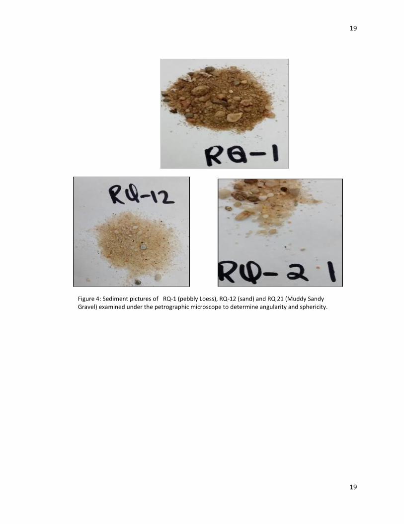
Figure 4: Sediment pictures of RQ-1 (pebbly Loess), RQ-12 (sand) and RQ 21 (Muddy Sandy Gravel) examined under the petrographic microscope to determine angularity and sphericity.

20
20
After obtaining angularity values, two dimensional images of the grains were analyzed for sphericity. Sphericity is defined as the nearness of a grain to a sphere; it can be described in terms of the relationship between the tree diameters of a grain-the Longest (dL), the shortest (ds) and an intermediate (dI). It is defined as the ratio of the surface area of the sphere having the same volume as the media grain to the surface area of the actual media grain (Logsdon, 2008). For a perfect sphere, the value of sphericity is 1, whereas for a cube it is 0.81.
(5b)
Figure 5a: Picture shows specimen set-up and Sample specimen of the grains observed under the petrographic microscope with a magnification of 31.5 (2.5 objective and 12.5x ocular to determine angularity and sphericity
21
21
Calculating sphericity (ψ) requires the measurement of ds (shortest axis), which is impractical for sand-size sediments viewed in a microscope (Al- Hashim, 2009). Riley’s sphericity, however, relies on measurements that can be taken from the two-dimensional view of a sand grain as seen through a microscope. The longest and the intermediate axis were measured to get a ratio using the Riley’s sphericity (Rψ) equation (Al-Hashim, 2009).
Rψ= (dI/dL) 0.5 eq. 8
Where, dI represents the intermediate axis and
dL represents the longest axis of the grain in Riley’s sphericity formula
Section 3: Results Based on visual analysis (figure 7), the sediment ranged from mud to gravel. Top 1.4 feet of the
core consisted of silty sand which could be pebbly loess; a common surface deposit in Suffolk County
ranging from a few centimeters to several meters in thickness (Kundic,2005). It is called pebbly loess due
to the presence of randomly distributed pebbles (Melrose, 2014). Below this top layer the sediments are
dominantly sands and gravels; consistent with glacial outwash.
Figure 6: Powers scale of roundness and sphericity chart.

22
22
Figure 7: Sedimentary log of core from Upper Glacial aquifer sediments on Suffolk Community College campus.

23
23
Section 3.1: grain-size sieve analysis, MasterSizer Results
Particle Size Distribution
0.01 0.1 1 10 100 1000 3000
Particle Size (µm)
0
1
2
3
4
5
Volu
me (%
)
RQ-1-second run-rerun - Average, Friday, December 05, 2014 2:18:33 PM
RQ-1-second run-rerun, Friday, December 05, 2014 2:19:51 PM
RQ-1-second run-rerun, Friday, December 05, 2014 2:19:12 PM
RQ-1-second run-rerun, Friday, December 05, 2014 2:18:33 PM
Figure 8: RQ-1 with bimodal grain-size distribution for pebbly loess at 2.3 feet depth.
Figure 9: RQ-3 grain-size distribution for coarse sand and gravel at 4 feet below surface.
Particle Size Distribution
0.01 0.1 1 10 100 1000 3000
Particle Size (µm)
0
2
4
6
8
10
Volu
me (
%)
RQ-3-second run, Friday, December 05, 2014 2:49:00 PM
RQ-3-second run, Friday, December 05, 2014 2:49:39 PM
RQ-3-second run, Friday, December 05, 2014 2:50:18 PM
RQ-3-second run - Average, Friday, December 05, 2014 2:49:00 PM
Particle Size Distribution
0.01 0.1 1 10 100 1000 3000
Particle Size (µm)
0
2
4
6
8
10
Volu
me (%
)
RQ-16-second run, Friday, December 05, 2014 7:22:35 PM
RQ-16-second run, Friday, December 05, 2014 7:23:15 PM
RQ-16-second run, Friday, December 05, 2014 7:23:54 PM
RQ-16-second run - Average, Friday, December 05, 2014 7:22:35 PM
Figure 10: RQ-16 grain-size distribution curve for unimodal fine to-medium grain sand at 22.6 feet below surface.

24
24
Figure 12: Grain-size distribution curves generated by the laser diffractometry for all 21 samples (RQ-1 to RQ-21).
Figure 11: RQ-21 sandy gravel grain-size distribution curve for bimodal distribution for a Muddy sandy gravel at 36 ft .below surface; the bottom of the core.
Particle Size Distribution
0.01 0.1 1 10 100 1000 3000
Particle Size (µm)
0
2
4
6
8 Volu
me (%
)
RQ-21-second run, Friday, December 05, 2014 8:45:13 PM
RQ-21-second run, Friday, December 05, 2014 8:45:52 PM
RQ-21-second run, Friday, December 05, 2014 8:46:31 PM
RQ-21-second run - Average, Friday, December 05, 2014 8:45:13 PM
25
25
Figure 8-figure 11 represents typical particle size distribution curves from the MasterSizer. Figure 12
shows a compilation of the 21 samples analyzed. Particle sizes range from 0.1 to 1000 microns and the
modes are at 10, 300, 500, 700 and 900 microns. Sample RQ-1; Pebbly Loess (Figure 8) has a polymodal
grain-size distribution and so do sandy gravel RQ-3 and RQ-21. Sample RQ- 16, which is mainly sand, has
a unimodal distribution. These are representative sediments found in the Upper Glacial Aquifer, Long
Island (Pine Barrens Overview, 2014).
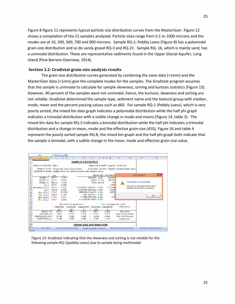
Section 3.2: Gradistat grain-size analysis results
The grain-size distribution curves generated by combining the sieve data (>1mm) and the
MasterSizer data (<1mm) give the complete modes for the samples. The Gradistat program assumes
that the sample is unimodal to calculate for sample skewness, sorting and kurtosis statistics (Figure 13).
However, 40 percent of the samples were not unimodal, hence, the kurtosis; skewness and sorting are
not reliable. Gradistat determined the sample type, sediment name and the textural group with median,
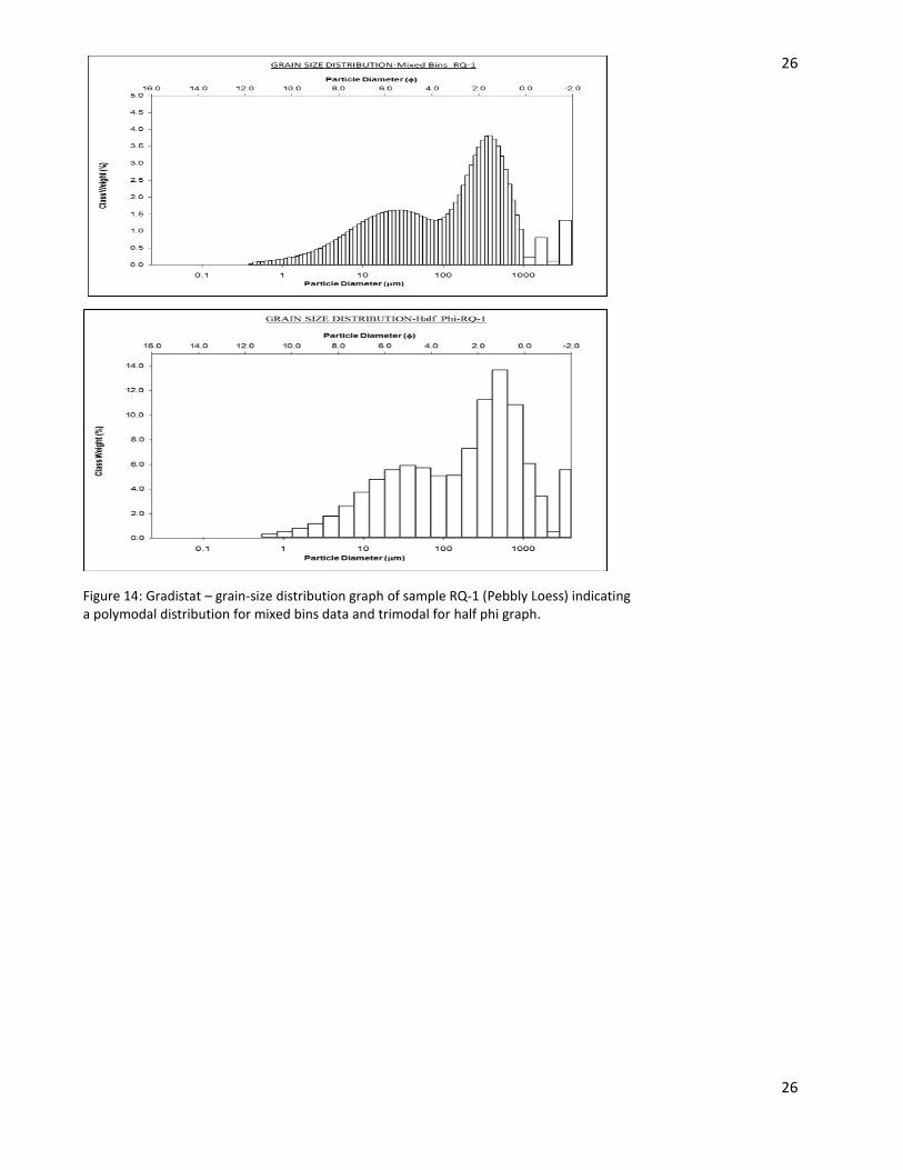
mode, mean and the percent passing values such as d60. For sample RQ-1 (Pebbly Loess), which is very
poorly sorted, the mixed bin data graph indicates a polymodal distribution while the half phi graph
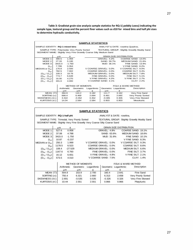
indicates a trimodal distribution with a visible change in mode and means (Figure 14, table 3). The
mixed-bin data for sample RQ-3 indicates a bimodal distribution while the half phi indicates a trimodal
distribution and a change in mean, mode and the effective grain-size (d10). Figure 16 and table 4
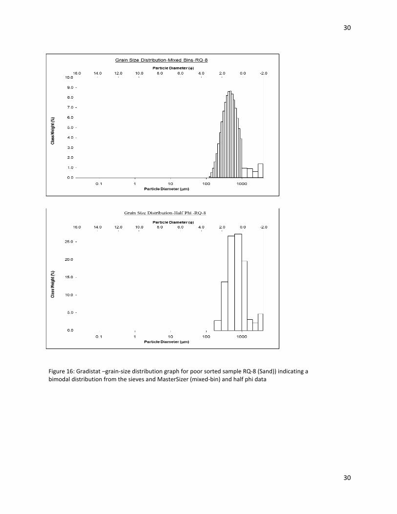
represent the poorly sorted sample RQ-8, the mixed bin graph and the half phi graph both indicate that
the sample is bimodal, with a subtle change in the mean, mode and effective grain-size value.
Figure 13: Gradistat indicating that the skewness and sorting is not reliable for the following sample-RQ-1(pebbly Loess) due to sample being multimodal
26
26
Figure 14: Gradistat – grain-size distribution graph of sample RQ-1 (Pebbly Loess) indicating a polymodal distribution for mixed bins data and trimodal for half phi graph.
27
27
Table 3: Gradistat grain-size analysis sample statistics for RQ-1( pebbly Loess) indicating the sample type, textural group and the percent finer values such as d10 for mixed bins and half phi sizes to determine hydraulic conductivity.
SAMPLE STATISTICS
SAMPLE IDENTITY: RQ-1-half phi ANALYST & DATE: roselina,
SAMPLE TYPE: Trimodal, Very Poorly Sorted TEXTURAL GROUP: Slightly Gravelly Muddy Sand
SEDIMENT NAME: Slightly Very Fine Gravelly Very Coarse Silty Coarse Sand
GRAIN SIZE DISTRIBUTION
MODE 1: GRAVEL: COARSE SAND: 19.1%
MODE 2: SAND: MEDIUM SAND: 18.6%
MODE 3: MUD: FINE SAND: 10.1%
D10: V FINE SAND: 8.3%
MEDIAN or D50: V COARSE GRAVEL: V COARSE SILT: 9.3%
D90: COARSE GRAVEL: COARSE SILT: 8.6%
(D90 / D10): MEDIUM GRAVEL: MEDIUM SILT: 6.6%
(D90 - D10): FINE GRAVEL: FINE SILT: 3.7%
(D75 / D25): V FINE GRAVEL: V FINE SILT: 2.1%
(D75 - D25): V COARSE SAND: CLAY: 1.4%
Logarithmic
f
MEAN : 2.700
SORTING (s): 2.660
SKEWNESS (Sk ): 0.535
KURTOSIS (K ): 2.551
750.4
1167.6
METHOD OF MOMENTS
f
0.958
4.788
-1.750
108.4
-0.237
1.999
2.691
10.44
mm
527.6
37.08
3415.0
10.87
250.3
1178.5
4.010
Arithmetic
mm
504.9
6.523
-27.529
6.760
Geometric
2.551
6.313
-0.326
0.866
mm
153.9
Platykurtic
Description
Fine Sand
Very Poorly Sorted
16.12
573.5
6.651
0.866
6.321
-0.535
7.5%
Geometric Logarithmic
Very Fine Skewed
f
0.326
mm
160.4 2.641
2.658
FOLK & WARD METHOD
4.8%
63.6%
31.6%
0.0%
0.0%
0.0%
0.0%
4.8%
)(x
SAMPLE STATISTICS
SAMPLE IDENTITY: RQ-1-mixed bins ANALYST & DATE: roselina Quadros,
SAMPLE TYPE: Polymodal, Very Poorly Sorted TEXTURAL GROUP: Slightly Gravelly Muddy Sand
SEDIMENT NAME: Slightly Very Fine Gravelly Coarse Silty Medium Sand
GRAIN SIZE DISTRIBUTION
MODE 1: GRAVEL: COARSE SAND: 13.0%
MODE 2: SAND: MEDIUM SAND: 21.6%
MODE 3: MUD: FINE SAND: 13.9%
D10: V FINE SAND: 8.2%
MEDIAN or D50: V COARSE GRAVEL: V COARSE SILT: 9.0%
D90: COARSE GRAVEL: COARSE SILT: 9.4%
(D90 / D10): MEDIUM GRAVEL: MEDIUM SILT: 7.8%
(D90 - D10): FINE GRAVEL: FINE SILT: 5.1%
(D75 / D25): V FINE GRAVEL: V FINE SILT: 2.7%
(D75 - D25): V COARSE SAND: CLAY: 2.2%
Logarithmic
f
MEAN : 3.182
SORTING (s): 2.694
SKEWNESS (Sk ): 0.452
KURTOSIS (K ): 2.584
699.4
774.7
METHOD OF MOMENTS
f
1.359
5.195
-1.750
100.3
0.354
2.500
3.310
14.04
mm
390.5
27.33
3415.0
7.799
176.8
782.5
4.000
Arithmetic
mm
394.9
7.002
19.79
6.649
Geometric
2.584
6.461
-0.305
0.903
mm
110.2
Mesokurtic
Description
Very Fine Sand
Very Poorly Sorted
16.00
401.6
4.270
0.903
6.469
-0.452
3.1%
Geometric Logarithmic
Very Fine Skewed
f
0.305
mm
111.7 3.162
2.692
FOLK & WARD METHOD
4.2%
59.7%
36.1%
0.0%
0.0%
0.0%
0.0%
4.2%
)(x

28
28
Figure 15: Gradistat –grain-size distribution graph for sample RQ-3(muddy sandy gravel) indicating a multimodal distribution from the sieves and MasterSizer data combined and half phi.

29
29
Table 4: Gradistat grain-size analysis sample statistics for RQ-3 (Muddy sandy gravel) Mixed Bin & Half phi indicating the sample type, textural group and the percent finer values such as d10 and d50 used to determine hydraulic conductivity.
SAMPLE STATISTICS
SAMPLE IDENTITY: RQ-3-half phi ANALYST & DATE: roselina,
SAMPLE TYPE: Trimodal, Poorly Sorted TEXTURAL GROUP: Muddy Sandy Gravel
SEDIMENT NAME: Coarse Silty Sandy Very Fine Gravel
GRAIN SIZE DISTRIBUTION
MODE 1: GRAVEL: COARSE SAND: 15.9%
MODE 2: SAND: MEDIUM SAND: 13.5%
MODE 3: MUD: FINE SAND: 5.7%
D10: V FINE SAND: 2.8%
MEDIAN or D50: V COARSE GRAVEL: V COARSE SILT: 3.0%
D90: COARSE GRAVEL: COARSE SILT: 3.2%
(D90 / D10): MEDIUM GRAVEL: MEDIUM SILT: 2.7%
(D90 - D10): FINE GRAVEL: FINE SILT: 1.9%
(D75 / D25): V FINE GRAVEL: V FINE SILT: 1.2%
(D75 - D25): V COARSE SAND: CLAY: 0.9%
Logarithmic
f
MEAN : 1.202
SORTING (s): 2.277
SKEWNESS (Sk ): 1.735
KURTOSIS (K ): 5.640
774.4
58768.9
METHOD OF MOMENTS
f
0.958
-1.750
5.427
1831.4
-5.878
0.045
2.499
9.144
mm
527.6
3415.0
23.82
32.11
969.0
58801.0
3.034
Arithmetic
mm
456.6
4.961
-0.844
10.84
Geometric
1.298
3.946
-0.710
0.926
mm
34.38
Mesokurtic
Description
Coarse Sand
Poorly Sorted
8.191
2255.8
-1.228
0.926
21.28
-0.065
6.4%
Geometric Logarithmic
Very Fine Skewed
f
0.710
mm
620.0 0.690
1.980
FOLK & WARD METHOD
42.9%
44.3%
12.8%
0.0%
0.0%
0.0%
0.0%
42.9%
)(x
SAMPLE STATISTICS
SAMPLE IDENTITY: RQ-3-mixed bins ANALYST & DATE: roselina Quadros,
SAMPLE TYPE: Bimodal, Poorly Sorted TEXTURAL GROUP: Muddy Sandy Gravel
SEDIMENT NAME: Fine Silty Sandy Very Fine Gravel
GRAIN SIZE DISTRIBUTION
MODE 1: GRAVEL: COARSE SAND: 16.1%
MODE 2: SAND: MEDIUM SAND: 22.5%
MODE 3: MUD: FINE SAND: 8.0%
D10: V FINE SAND: 0.9%
MEDIAN or D50: V COARSE GRAVEL: V COARSE SILT: 0.8%
D90: COARSE GRAVEL: COARSE SILT: 0.8%
(D90 / D10): MEDIUM GRAVEL: MEDIUM SILT: 1.1%
(D90 - D10): FINE GRAVEL: FINE SILT: 1.2%
(D75 / D25): V FINE GRAVEL: V FINE SILT: 1.0%
(D75 - D25): V COARSE SAND: CLAY: 1.0%
Logarithmic
f
MEAN : 0.963
SORTING (s): 1.917
SKEWNESS (Sk ): 2.420
KURTOSIS (K ): 10.38
FOLK & WARD METHOD
43.3%
50.6%
6.1%
0.0%
0.0%
0.0%
0.0%
43.3%
3.1%
Geometric Logarithmic
Very Fine Skewed
f
0.457
mm
721.0 0.472
1.541
Platykurtic
Description
Coarse Sand
Poorly Sorted
7.221
2192.8
-1.116
0.798
21.73
-0.213
1.272
2.909
-0.457
0.798
mm
39.54
Arithmetic
mm
446.3
2.389
-0.442
7.794
Geometric
2.733
10.28
mm
436.3
3415.0
190.9
787.0
42375.0
2.852
756.0
42184.0
METHOD OF MOMENTS
f
1.199
-1.750
221.9
-5.405
0.346
)(x
30
30
Figure 16: Gradistat –grain-size distribution graph for poor sorted sample RQ-8 (Sand)) indicating a bimodal distribution from the sieves and MasterSizer (mixed-bin) and half phi data

31
31
For sample R-2, RQ-4, 5, 6, 7, 9-21, particle size distribution graphs and statistics please refer to
appendices
Section 3.3: Shape and Angularity results from the microscopic experiment
The shape, sphericity and angularity of grains were determined using the Riley’s two dimensional formula and Powers Roundness chart for angularity. In the following figure (Figure 17) for sample RQ-1 and RQ-3 the shape of the grains can be seen (refer to appendix for RQ-4-RQ 21). The grains range from very angular to sub angular in shape (1.88-2.52).
SAMPLE STATISTICS
SAMPLE IDENTITY: RQ-8-half phi ANALYST & DATE: roselina,
SAMPLE TYPE: Bimodal, Poorly Sorted TEXTURAL GROUP: Gravelly Sand
SEDIMENT NAME: Very Fine Gravelly Coarse Sand
GRAIN SIZE DISTRIBUTION
MODE 1: GRAVEL: COARSE SAND: 39.3%
MODE 2: SAND: MEDIUM SAND: 23.8%
MODE 3: MUD: FINE SAND: 2.3%
D10: V FINE SAND: 0.0%
MEDIAN or D50: V COARSE GRAVEL: V COARSE SILT: 0.0%
D90: COARSE GRAVEL: COARSE SILT: 0.0%
(D90 / D10): MEDIUM GRAVEL: MEDIUM SILT: 0.0%
(D90 - D10): FINE GRAVEL: FINE SILT: 0.0%
(D75 / D25): V FINE GRAVEL: V FINE SILT: 0.0%
(D75 - D25): V COARSE SAND: CLAY: 0.0%
Logarithmic
f
MEAN : 0.449
SORTING (s): 0.810
SKEWNESS (Sk ): -0.308
KURTOSIS (K ): 3.516
671.7
4094.4
METHOD OF MOMENTS
f
0.319
-1.750
12.95
-2.150
0.389
2.237
9.391
mm
821.2
3415.0
342.7
763.5
4437.1
1.365
Arithmetic
mm
749.2
1.545
-0.719
3.694
Geometric
5.135
2.145
0.144
0.766
mm
293.1
Platykurtic
Description
Coarse Sand
Poorly Sorted
2.575
772.2
-3.058
0.766
9.851
-1.910
16.4%
Geometric Logarithmic
Coarse Skewed
f
-0.144
mm
988.4 0.017
1.101
FOLK & WARD METHOD
18.2%
81.8%
0.0%
0.0%
0.0%
0.0%
0.0%
18.2%
)(x
Table 5: Gradistat grain-size analysis sample statistics for RQ-8 mixed bin & half phi indicating the sample type, textural group and the percent finer values such as d10 and d50 used to determine hydraulic conductivity.
SAMPLE STATISTICS
SAMPLE IDENTITY: RQ-8mixed bins ANALYST & DATE: roselina Quadros,
SAMPLE TYPE: Bimodal, Poorly Sorted TEXTURAL GROUP: Gravelly Sand
SEDIMENT NAME: Very Fine Gravelly Medium Sand
GRAIN SIZE DISTRIBUTION
MODE 1: GRAVEL: COARSE SAND: 32.0%
MODE 2: SAND: MEDIUM SAND: 36.2%
MODE 3: MUD: FINE SAND: 8.9%
D10: V FINE SAND: 0.0%
MEDIAN or D50: V COARSE GRAVEL: V COARSE SILT: 0.0%
D90: COARSE GRAVEL: COARSE SILT: 0.0%
(D90 / D10): MEDIUM GRAVEL: MEDIUM SILT: 0.0%
(D90 - D10): FINE GRAVEL: FINE SILT: 0.0%
(D75 / D25): V FINE GRAVEL: V FINE SILT: 0.0%
(D75 - D25): V COARSE SAND: CLAY: 0.0%
Logarithmic
f
MEAN : 0.812
SORTING (s): 0.936
SKEWNESS (Sk ): -0.555
KURTOSIS (K ): 3.406
FOLK & WARD METHOD
18.2%
81.8%
0.0%
0.0%
0.0%
0.0%
0.0%
18.2%
4.6%
Geometric Logarithmic
Coarse Skewed
f
-0.299
mm
789.4 0.341
1.283
Platykurtic
Description
Coarse Sand
Poorly Sorted
2.583
567.1
13.23
0.887
9.104
-1.817
4.982
2.433
0.299
0.887
mm
228.0
Arithmetic
mm
593.7
1.954
-0.902
4.121
Geometric
2.875
11.96
mm
487.4
3415.0
258.1
541.0
4491.4
1.369
668.3
4233.3
METHOD OF MOMENTS
f
1.039
-1.750
17.40
-2.167
0.886
)(x
32
32
RQ1- Pebbly Loess (clay, silt, sand, gravel) RQ3-Poorly sorted Muddy Sandy Gravel
Figure 17: Angularity and shape results of grain shape analyses for sample RQ-1 (Pebbly Loess) and RQ-3 (muddy sandy gravel) to determine angularity and sphericity

33
33
Table 6: Angularity and sphericity results using the Riley’s formula to calculate sphericity and Power’s chart to determine angularity. Where dI is the intermediate axis and the longest axis is dL
Sample name Angularity dL dI dI/dL Sphericity
RQ-1 2.52 14.84 10.04 0.684 0.8225
RQ-2 2.52 13.16 8.2 0.622 0.7888
RQ-3 2.4 10.52 7.12 0.658 0.8110
RQ-4 2.16 9.48 6.28 0.654 0.8087
RQ-5 2.52 11.88 7.8 0.650 0.8062
RQ-6 2.28 9.32 6.16 0.689 0.8303
RQ-7 2.2 9.44 5.6 0.616 0.7848
RQ-8 2.36 10.32 7.36 0.720 0.8485
RQ-9 2.24 9.68 6.16 0.662 0.8134
RQ-10 2.4 12.92 8.96 0.696 0.8344
RQ-11 1.88 8.24 5.36 0.684 0.8222
RQ-12 2.28 20.08 13.28 0.675 0.8157
RQ-13 2.36 15.2 11 0.723 0.8453
RQ-14 2.36 14.12 10.44 0.735 0.8518
RQ-15 2.36 11.52 8.08 0.692 0.8321
RQ-16 2.36 11.72 8.56 0.728 0.8506
RQ-17 2.24 11 6.96 0.655 0.8004
RQ-18 2.28 12.84 8.56 0.690 0.8238
RQ-19 2.12 11.08 7.08 0.639 0.7902
RQ-20 2.2 12.44 8.52 0.669 0.8122
RQ-21 2 10.08 6 0.615 0.7720
34
34
The sand grains are angular to sub angular in nature and have a calculated sphericity of 0.817. A perfect
sphere has a sphericity of 1. Logsdon (2008), states that sphericity values for silica sand typically range
from 0.7 – 0.8. This sphericity indicates that the sediments have not been transported far from the
source area. According to Blanco (2003) poorly sorted, angular, non-spherical particles tend not to pack
as neatly as well sorted, rounded, spherical particles and the void spaces are filled with smaller grains
reducing the flow of fluid through the medium. While the hydraulic conductivity equations do not take
angularity and shape into account, it is assumed that the calculated hydraulic conductivity values are
maximum values.
Section 3.4: Hydraulic conductivity for samples with unimodal grain-size distributions.
The Gradistat program gives the parameters needed to calculate the hydraulic conductivity;
however Gradistat assumes that the grain-size distribution is unimodal. For the 21 samples, the grain-
size distribution range from unimodal to multimodal; the unimodal samples are moderately sorted while
the multimodal samples are poorly sorted. According to (Franke et al .1972), the average hydraulic
conductivity for the Upper Glacial Aquifer on Long Island is 240 ft/d. The Upper Glacial aquifer consists
of sediments deposited during the last glaciation and consisting mainly of sand and gravel with minor silt
(Pine Barrens, 2014). Doriski et al. (1993) found hydraulic conductivity values that range from 107 to 343
ft/d based on grain-size analysis using the sieving method.
The computed hydraulic conductivity parameters and the hydraulic conductivity for each
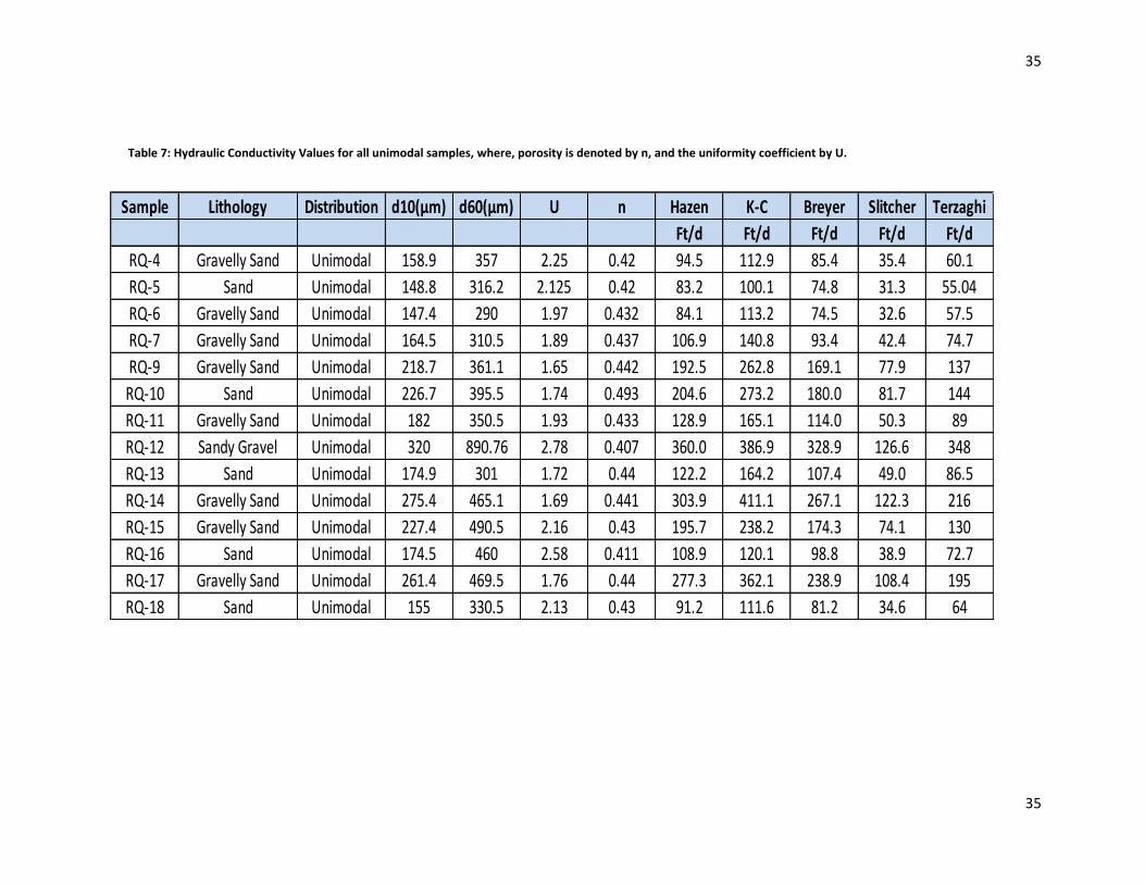
method for unimodal samples are shown in Table 7. Table 7 gives the average hydraulic conductivity
estimated from Hazen, Kozeny-Carman, Slitcher, Breyer and Terzaghi method for all 21 samples. Figure
18 gives a graphical representation of Table 8, where average conductivity is plotted against the
statistical methods.
35
35
Table 7: Hydraulic Conductivity Values for all unimodal samples, where, porosity is denoted by n, and the uniformity coefficient by U.
Sample Lithology Distribution d10(μm) d60(μm) U n Hazen K-C Breyer Slitcher Terzaghi
Ft/d Ft/d Ft/d Ft/d Ft/d
RQ-4 Gravelly Sand Unimodal 158.9 357 2.25 0.42 94.5 112.9 85.4 35.4 60.1
RQ-5 Sand Unimodal 148.8 316.2 2.125 0.42 83.2 100.1 74.8 31.3 55.04
RQ-6 Gravelly Sand Unimodal 147.4 290 1.97 0.432 84.1 113.2 74.5 32.6 57.5
RQ-7 Gravelly Sand Unimodal 164.5 310.5 1.89 0.437 106.9 140.8 93.4 42.4 74.7
RQ-9 Gravelly Sand Unimodal 218.7 361.1 1.65 0.442 192.5 262.8 169.1 77.9 137
RQ-10 Sand Unimodal 226.7 395.5 1.74 0.493 204.6 273.2 180.0 81.7 144
RQ-11 Gravelly Sand Unimodal 182 350.5 1.93 0.433 128.9 165.1 114.0 50.3 89
RQ-12 Sandy Gravel Unimodal 320 890.76 2.78 0.407 360.0 386.9 328.9 126.6 348
RQ-13 Sand Unimodal 174.9 301 1.72 0.44 122.2 164.2 107.4 49.0 86.5
RQ-14 Gravelly Sand Unimodal 275.4 465.1 1.69 0.441 303.9 411.1 267.1 122.3 216
RQ-15 Gravelly Sand Unimodal 227.4 490.5 2.16 0.43 195.7 238.2 174.3 74.1 130
RQ-16 Sand Unimodal 174.5 460 2.58 0.411 108.9 120.1 98.8 38.9 72.7
RQ-17 Gravelly Sand Unimodal 261.4 469.5 1.76 0.44 277.3 362.1 238.9 108.4 195
RQ-18 Sand Unimodal 155 330.5 2.13 0.43 91.2 111.6 81.2 34.6 64

36
36
The hydraulic conductivities for the unimodal sediments calculated using the Slitcher method are lower
than for other methods, which is consistent with the findings of Vukovic and Soro (1992) and Cheng and
Chen (2007). Odong (2013) stated that Slitcher method is invariably inaccurate. Kozeny-Carman method
gave the highest mean value followed by Hazen. Hazen and Kozeny-Carman are considered as the best
method for calculating the hydraulic conductivity of uniform sediments (Odong, 2013). This can be
attributed to the fact that Kozeny Carman can be used for most soil textures and it is the most widely
accepted and used empirical method. Average conductivity by Hazen, Kozeny-Carman, Breyer and
Terzaghi gave similar values. The Terzaghi method is known to work well for larger grain-size sediments
such as sand and gravel (Odong, 2013). Therefore, the use of this method may be effective for outwash
sediments the mean conductivity values computed (Table 8) by different methods indicate the hydraulic
conductivity of unimodal sand, sandy gravel, and gravelly sand.
The suitable methods for calculating unimodal sediments hydraulic conductivity were Kozeny-Carman
followed by Hazen, Breyer and Terzaghi based on the results. All methods are based on the same
effective grain-size (d10), however they generate different results. This is due to the use of different
constant values for Hazen, Kozeny-Carman, and Slitcher. For Terzaghi the results may be a reflection of
the average value of coarser and finer empirical coefficient value. Breyer method uses the uniformity
coefficient to calculate the hydraulic conductivity in the equation along with porosity, in contrast to the
rest of the methods that only use porosity value which is derived from the uniformity coefficient value.
Hence, contributing to the estimated results for the Breyer method. Among the suitable methods,
Kozeny-Carman and Hazen gave average conductivity values consistent with the upper glacial aquifer
hydraulic conductivity which is about 240 ft/d. In this study, the best method to calculate the hydraulic
conductivity of the unimodal sediments would be Kozeny-Carman since it is known to work well with
most soil textures excluding clayey soils (Aguilar, 2013) and generates conductivity value very close to
the estimated hydraulic conductivity of the upper glacial aquifer. Hazen may not be highly effective
since it is only good for uniform sand and the study samples are not uniform (Odong, 2013).
Table 8: Average of hydraulic conductivity of Unimodal Sediments from different statistical grain-size methods
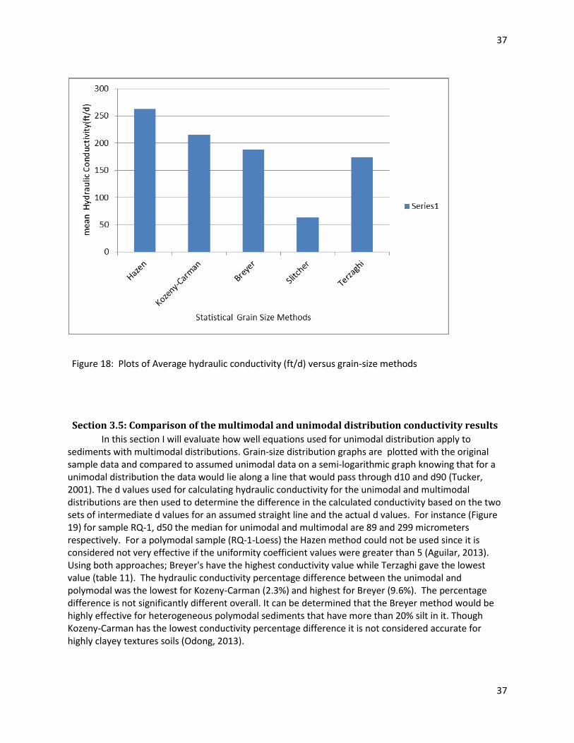
37
37
Section 3.5: Comparison of the multimodal and unimodal distribution conductivity results
In this section I will evaluate how well equations used for unimodal distribution apply to sediments with multimodal distributions. Grain-size distribution graphs are plotted with the original sample data and compared to assumed unimodal data on a semi-logarithmic graph knowing that for a unimodal distribution the data would lie along a line that would pass through d10 and d90 (Tucker, 2001). The d values used for calculating hydraulic conductivity for the unimodal and multimodal distributions are then used to determine the difference in the calculated conductivity based on the two sets of intermediate d values for an assumed straight line and the actual d values. For instance (Figure 19) for sample RQ-1, d50 the median for unimodal and multimodal are 89 and 299 micrometers respectively. For a polymodal sample (RQ-1-Loess) the Hazen method could not be used since it is considered not very effective if the uniformity coefficient values were greater than 5 (Aguilar, 2013). Using both approaches; Breyer's have the highest conductivity value while Terzaghi gave the lowest value (table 11). The hydraulic conductivity percentage difference between the unimodal and polymodal was the lowest for Kozeny-Carman (2.3%) and highest for Breyer (9.6%). The percentage difference is not significantly different overall. It can be determined that the Breyer method would be highly effective for heterogeneous polymodal sediments that have more than 20% silt in it. Though Kozeny-Carman has the lowest conductivity percentage difference it is not considered accurate for highly clayey textures soils (Odong, 2013).
Figure 18: Plots of Average hydraulic conductivity (ft/d) versus grain-size methods
38
38
For bimodal muddy gravelly sand (RQ-3), the hydraulic conductivity range from 30.2 ft/d to 96.6 ft/d for bimodal approach, while for unimodal approach it ranges from 21.3 ft/d to 99.32 ft/d. By using both approaches; Breyer gives the highest conductivity value, followed by Kozeny-Carman and then Terzaghi. The conductivity percentage difference between the two approaches is the lowest (2.9%) for Breyer and highest for Terzaghi (34.5%). Further, for bimodal gravelly sand, the hydraulic conductivity range from 115 ft/d to 216.3 ft/d using the unimodal approach, while it is 197 ft/d to 307.28 ft/d for multimodal approach. In both cases, Terzaghi underestimates the conductivity value. For unimodal, Hazen gives the highest conductivity value and for multimodal, Kozeny-Carman has the highest value. The percentage difference is lowest for Breyer and highest for Terzaghi.
The hydraulic conductivity for a trimodal sandy gravel (RQ-19), ranged from 14.9 ft/d to 122.7 ft/d using unimodal approach and 29 ft/d to 120 ft /d for trimodal approach. In both approaches, Terzaghi gives the lowest conductivity value with the highest percentage difference (64.5%). While Breyer's method give the lowest percentage difference (0.42%). The percentage difference between Breyer and Terzaghi is significantly high. Lastly, for bimodal muddy sandy gravel (RQ-21) the percentage difference is lowest for Breyer (2.12%), followed by Kozeny-Carman (9%). Terzaghi has the highest hydraulic conductivity percentage difference (44.5%). The conductivity value is highest for Breyer in both approaches while it is the lowest for Terzaghi in Unimodal approach .There is a significant difference between Breyer and Terzaghi.
It can be seen that the hydraulic conductivity value for Terzaghi for bimodal, trimodal and polymodal samples, is higher than unimodal. From this experiment it can be inferred that Breyer and Kozeny-Carman method are most effective for bimodal muddy gravelly sand since it has the lowest hydraulic conductivity percentage difference. In contrast, Breyer and Hazen would be more effective in the calculation of hydraulic conductivity of bimodal gravelly sand and trimodal sandy gravel. The Breyer method has been known to work best on heterogeneous sediments hence the lower conductivity percentage difference and a reasonable hydraulic conductivity value may be attributed to this reason (Odong, 2013). Furthermore, Kozeny-Carman can be used for most soil textures except given the sediment type is not very clayey (Odong, 2013).
39
39
Table 10: Average of hydraulic conductivity of Multimodal Sediments from different statistical grain-size methods
Table 9: Hydraulic Conductivity Values for all multimodal samples, where, porosity is denoted by n, and the uniformity coefficient by U.
Sample Lithology Distribution d10(μm) d60(μm) U n Hazen K-C Breyer Slitcher Terzaghi
Ft/d Ft/d Ft/d Ft/d Ft/d
RQ-1 Loess Polymodal 10.0 364 36.4 0.255 NA 0.0723 0.193 0.0270 0.047
RQ-2 Loess Bimodal 9.25 91.2 11.2 0.124 NA 0.0328 0.0156 0.00164 0.00051
RQ-3 Sandy Gravel Bimodal 197 514 8.88 0.304 NA 44.3 96.6 18.4 80.2
RQ-8 Gravelly Sand Bimodal 267 631 2.36 0.419 263 307 236 97.2 197
RQ-19 Sandy Gravel Trimodal 152 831 5.50 0.350 NA 44.4 64.1 16.8 29
RQ-20 Gravelly Muddy Sand Bimodal 20.2 365 18.0 0.260 NA 0.274 0.842 0.131 0.182
RQ-21 Muddy Sandy Gravel Bimodal 101 985 9.85 0.296 NA 10.3 24.3 4.34 12.6

40
40
Table 11: RQ- 1 sample results hydraulic Conductivity percentage difference using unimodal and multimodal approach
Figure 19: sample RQ-1 (polymodal-Pebbly Loess) Results- depicting the unimodal and multimodal distribution difference.

41
41
Table 12: RQ- 3 sample results hydraulic Conductivity percentage difference using unimodal and multimodal approach
Figure 20: Sample RQ-3 (Muddy sandy gravel) depicting the difference in unimodal and multimodal parameters to calculate the hydraulic conductivity.

42
42
Figure 21: sample RQ-8 (Gravelly sand) results depicting the percentage difference between the unimodal and multimodal distribution in determining the hydraulic conductivity.
Table 13: Sample RQ-8 results - hydraulic Conductivity percentage difference using unimodal and multimodal approach on a same sample

43
43
Table 14: RQ-19 sample results - hydraulic conductivity percentage difference using unimodal and multimodal approach on a same sample
Figure 22: RQ-19 (Sandy Gravel at 32 feet below ground sample results showing the Conductivity difference between the unimodal and multimodal distribution

44
44
The hydraulic conductivity for the complete core based on the results is as follows:
Hazen: 174.5 ft/d (2nd best suitable method for unimodal sediments the value may be inaccurate
since it was not used for some multimodal samples
Kozeny-Carman: 160.4 ft/d (1st best suitable method for unimodal sediments)
Breyer: 119.5 ft/d (1st best suitable method for multimodal and 3rd best suitable method for
unimodal)
Terzaghi: 97.6 ft/d (3rd best suitable method for multimodal sediments and 4th for unimodal)
Slitcher: 49.6 ft/d (known to be inaccurate according (Odong, 2013), and is not effective in the
calculations of hydraulic conductivity for unimodal and multimodal sediments.
Figure 23: RQ-21 (Muddy Sandy Gravel at 36 feet below ground) sample results showing the conductivity difference between the unimodal and multimodal distribution
Table 15: sample RQ-21 results showing hydraulic conductivity percentage difference using the unimodal and multimodal distribution approach on a same sample

45
45
Section 3.6: Variations in hydraulic conductivity using different empirical methods
All the empirical methods used in this study use 3 variables, which are Temperature, U and d10
values. U is used to calculate the porosity, which is used in all the equations except Breyer. Figure 24- 28
represents plots of temperature (T) against the g/v value (figure 24) and U versus the f (n) term (figure
25) in each of the empirical method respectively. It can be seen that 1 degree increase in temperature
leads to a 3.3 percent increase in the g/v value for a sample. Where, kinematic viscosity (v) is
dependent on dynamic viscosity and the density of the fluid. The density changes with temperature in
calculating the kinematic viscosity. However, the viscosity is much more sensitive to temperature than
the density. Temperature is not very important, since it is fixed as well as U. However, d10 is crucial in
the calculation of conductivity value. It can be determined that the f (n) term in each method
determines how U is used to calculate the conductivity value. Furthermore, for each method, as the
value of uniformity coefficient (U) increases the f(n) term decreases, independent of how it is structured
in the equation (refer to figure 25 -28). Figure 33 gives a relationship between (d10)2 and f (n) term, as
(d10) ^2 increases f (n) value decreases. The f (n) term is based on U and some constants and U intern is
based on d10 and d60, hence an increase in d10 leads to a decrease in the f (n) value.
As seen in figure 29 and 30, U does not have a direct relationship with the hydraulic conductivity hence
it is not controlling it. However, a variable that controls the hydraulic conductivity the d10 value, as seen
in figure 31 and 32. The d10 value has a direct relationship with hydraulic conductivity and it controls it.
Hydraulic conductivity increases as d10 value increases.
Figure 24: shows a plot of temperature vs. g/v –As temperature increases g/v value increases
Figure 25: shows a plot of U vs. Cn term for Hazen's method

46
46
Figure 26: shows a plot of U vs. Cn term for Kozeny-Carman method
Figure 27: shows a plot of U vs. Cn term for Breyer Method
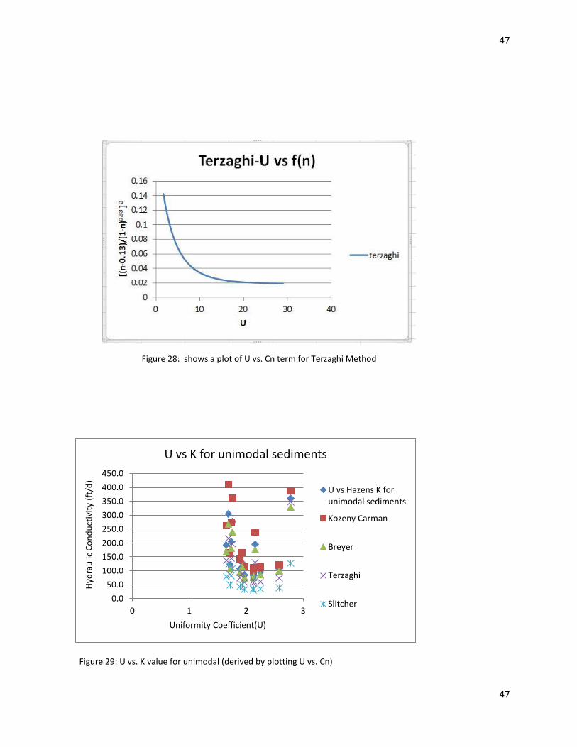
47
47
Figure 28: shows a plot of U vs. Cn term for Terzaghi Method
Figure 29: U vs. K value for unimodal (derived by plotting U vs. Cn)
0.0
50.0
100.0
150.0
200.0
250.0
300.0
350.0
400.0
450.0
0 1 2 3
Hyd
rau
lic C
on
du
ctiv
ity
(ft/
d)
Uniformity Coefficient(U)
U vs K for unimodal sediments
U vs Hazens K forunimodal sediments
Kozeny Carman
Breyer
Terzaghi
Slitcher

48
48
Figure 30: U vs. K value for multimodal (derived by plotting U vs. Cn)
0.0000
50.0000
100.0000
150.0000
200.0000
250.0000
300.0000
350.0000
0 5 10 15 20 25 30 35 40
Hyd
rau
lic C
on
du
ctiv
ity(
ft/
d)
Uniformity Coefficient (U)
U vs K for multimodal sediments
U vs KozenyCarman's K
U vs Breyers K
U vs Terzaghi's K
Figure 31: d10 vs. K value for unimodal sediments showing a direct relationship between the d10 and K. As d10 increases K increases.
0.0
50.0
100.0
150.0
200.0
250.0
300.0
350.0
400.0
450.0
0 50 100 150 200 250 300 350
hyd
rau
lic c
on
du
ctiv
ity(
ft/d
)
d10
d10 vs K for unimodal sediments
d10 vs K forHazen
d10 vs K forKozeny-Carmand10 vs K forBreyer
d10 vs K forSlitcher
d0 vs K forterzaghi

49
49
0
50
100
150
200
250
300
350
0.0 50.0 100.0 150.0 200.0 250.0 300.0
Hyd
rau
lic C
on
du
ctiv
ity
(ft/
d)
d10
d10 vs K for multimodal sediments
d10 vs K -Breyer
Kozeny-Carman
Terzaghi
Figure 32: d10 vs. K value for multimodal sediments showing a direct relationship between d10 and K. As d10 increases conductivity increases.
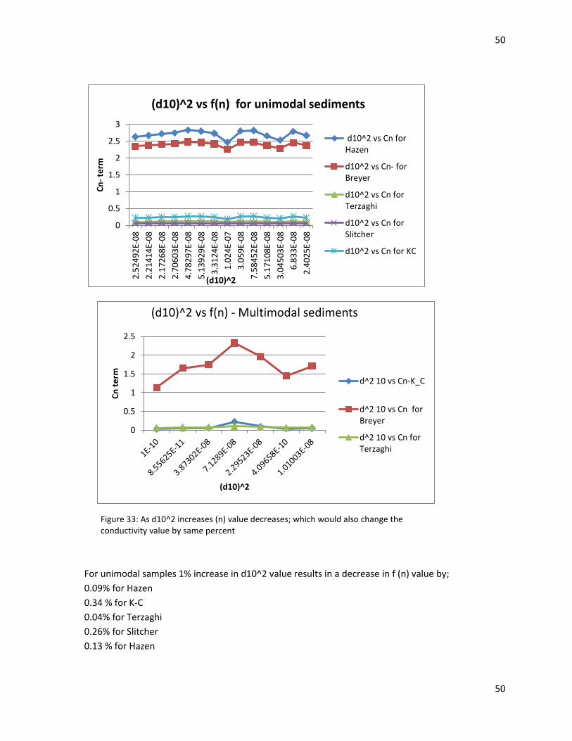
50
50
For unimodal samples 1% increase in d10^2 value results in a decrease in f (n) value by;
0.09% for Hazen
0.34 % for K-C
0.04% for Terzaghi
0.26% for Slitcher
0.13 % for Hazen
0
0.5
1
1.5
2
2.5
Cn
te
rm
(d10)^2
(d10)^2 vs f(n) - Multimodal sediments
d^2 10 vs Cn-K_C
d^2 10 vs Cn forBreyer
d^2 10 vs Cn forTerzaghi
0
0.5
1
1.5
2
2.5
32
.52
49
2E-
08
2.2
14
14
E-0
8
2.1
72
68
E-0
8
2.7
06
03
E-0
8
4.7
82
97
E-0
8
5.1
39
29
E-0
8
3.3
12
4E-
08
1.0
24
E-0
7
3.0
59
E-0
8
7.5
84
52
E-0
8
5.1
71
08
E-0
8
3.0
45
03
E-0
8
6.8
33
E-0
8
2.4
02
5E-
08
Cn
- te
rm
(d10)^2
(d10)^2 vs f(n) for unimodal sediments
d10^2 vs Cn forHazen
d10^2 vs Cn- forBreyer
d10^2 vs Cn forTerzaghi
d10^2 vs Cn forSlitcher
d10^2 vs Cn for KC
Figure 33: As d10^2 increases (n) value decreases; which would also change the conductivity value by same percent

51
51
Whereas, for multimodal samples
1% increase in the d10^2 value results in the decrease in f (n) value by;
0.03% for Breyer
0.10% for K-C
0.04 % for Terzaghi (which is the same as unimodal sediments % for Terzaghi)
Section 4 Discussion: When methods developed for unimodal sediments are used on sediments having a multimodal grain-
size distribution, it creates a discrepancy in the calculated hydraulic conductivity value. The difference in
calculated hydraulic conductivity using the unimodal approach can give greater or lower values based on
the sediment type. After comparing the grain-size distribution plots of assumed unimodal approach to
multimodal approach for the same sample, it can be seen that the slope (d75/d25) or d60/d10 in the
plot plays a significant role in the estimation of calculated hydraulic conductivity. As seen in figure 21,
the hydraulic conductivity is less using the multimodal approach on the slope of the straight line of
multimodal curve. In figure 19, the conductivity is greater using the unimodal approach, however, if the
slope of the multimodal line is considered, then the hydraulic conductivity prediction is better than
unimodal because of the slope (d60/d10). For figure 21, using the d75/d25 slope value for conductivity
estimation gets a higher value then using the d60/d10 slope. Hence, it is easier to predict the
conductivity of the slope derived from a single straight line instead of a curve as seen in figure 21.
On analysis of all the methods, the best method to be used for multimodal sediments could not be
selected since all the methods use the same factors and values. The difference among the various
methods is the structure of the porosity function (f (n)). The angularity and sphericity may be factors
that contribute to the actual hydraulic conductivity; however, the methods used in this research did not
include the angularity and sphericity values directly in the equation to calculate the conductivity. In Fig.
19-23, it can be seen that the use of percent finer values of 75% or less is more important and the
methods are all based on these values. While, on the other hand it is not known whether the modes
formed beyond 1mm grain-sizes are relevant in the conductivity estimation. That is if, coarser material
has an impact on the hydraulic conductivity. More studies would need to be done to see its effect on the
hydraulic conductivity and how it plays a role.
In the research area, 65 % of the core samples are made up of unimodal sediments while 35 % are
multimodal sediments. The unimodal sediments consist of slightly gravelly sand, gravelly sand, sand and
sandy gravel. The multimodal samples are pebbly loess, muddy sandy gravel, gravelly muddy sand,
sandy gravel and gravelly sand. Hence it can be understood that the water flow through each sediment
type would not be consistent for the upper glacial aquifer. The water flow is slower in units at a depth of
30-36 feet where silt exists along with sand and gravel. Through the sandy gravel the flow of water is
little slower than gravelly sand which has the highest conductivity. It can be inferred from the results
that the hydraulic conductivity of the section is governed by the sediments having a higher conductivity.

52
52
References Cited Aguilar, J.R., 2013. Analysis of Grain-size Distribution and Hydraulic Conductivity for a Variety of
Sediment Types with Application to Wadi Sediments: Master’s Thesis- King Abdullah University of Science and Technology, Saudi Arabia
Alayemi M.S., Sen, Z., 1993. Ground Water: Determination of hydraulic conductivity from complete
grain-size distribution curves. Vol 31, No.4, p. 1-10.
Al-Hashim, M., 2009.Sedimentary Petrology: Grain Morphology, Personal communication.
Aquitard System Hydrologically Connected to River. Hydrogeology Journal. 15: p.669-678
Beuselinck, L., Govers, G., Poesen, J., Degreaser, G., and Froyen, L., 1998. Grain- size Analysis by laser diffractometry: Comparison with the sieve- pipette method: Catena, v. 32, p. 193- 208.
Blanco, B.L., 2003.Dynamics of gravel and mixed, sand and gravel, beaches: Master’s Thesis-Imperial College of Science Technology and Medicine, London UK.
Blott, S.J., and Pye, K., 2001, Gradistat: A grain distribution and statistics package for the analysis of unconsolidated sediments: Earth Surface Processes and Landforms, vol. 26, 1234-1247.
Busciolano, R., 2002.Water Table and potentiometric altitudes of the upper glacial, Magothy, and Lloyd aquifers on long Island, New York: USGS-Water Resources Investigation report 1-4165.
Cheng, C., and Chen, X., 2007: Evaluation of Methods for Determination of Hydraulic Properties in an Aquifer.
Carman, P.C., 1937 "Fluid flow through granular beds." Transactions, Institution of Chemical Engineers, London, Vol.15: p. 150-166.
Dominguez, K., 2014: Grain-size analysis and soil stratigraphy across Suffolk County: Proxy for classification of sediment as a Diamict. Master’s Thesis at Stony Brook University.
Domenico, P.A. and F.W. Schwartz, 1990. Physical and Chemical Hydrogeology, John Wiley & Sons, New York, p.824.
Dias, K.A., 2014: High-Resolution Methodology for Particle Size Analysis of Naturally Occurring Sand Size Sediment through Laser Diffractometry with Application to Sediment Cores: Kismet, Fire Island, New York, p 1-55.
Doriski, T., Husain, S., Davis, S., Tsang-Rakovan, M, M., 1993. Comparison of hydraulic conductivity values Determined by Aquifer tests, specific capacity tests, slug tests, and grain-size analysis, https://dspace.sunyconnect.suny.edu/bitstream/handle/1951/47838/DORISK00.pdf?sequence=1 p.31-38.
EngineeringToolbox. Density of Fluids-changing Pressure and Temperature: Engineeringtoolbox http://www.engineeringtoolbox.com/fluid- -temperature-pressure-d_309.html
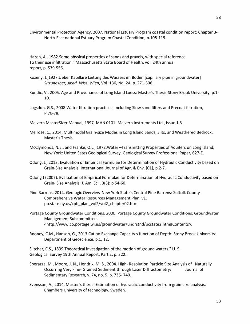
53
53
Environmental Protection Agency. 2007. National Estuary Program coastal condition report: Chapter 3-North-East national Estuary Program Coastal Condition, p.108-119.
Hazen, A., 1982.Some physical properties of sands and gravels, with special reference To their use infiltration." Massachusetts State Board of Health, vol. 24th annual report, p. 539-556.
Kozeny, J.,1927.Ueber Kapillare Leitung des Wassers im Boden [capillary pipe in groundwater] Sitzungsber, Akad. Wiss. Wien, Vol. 136, No. 2A, p. 271-306.
Kundic, V., 2005. Age and Provenance of Long Island Loess: Master’s Thesis-Stony Brook University, p.1-10.
Logsdon, G.S., 2008.Water filtration practices: Including Slow sand filters and Precoat filtration, P.76-78.
Malvern MasterSizer Manual, 1997. MAN 0101: Malvern Instruments Ltd., Issue 1.3.
Melrose, C., 2014, Multimodal Grain-size Modes in Long Island Sands, Silts, and Weathered Bedrock: Master’s Thesis.
McClymonds, N.E., and Franke, O.L., 1972.Water –Transmitting Properties of Aquifers on Long Island, New York: United Sates Geological Survey, Geological Survey Professional Paper, 627-E.
Odong, J., 2013. Evaluation of Empirical Formulae for Determination of Hydraulic Conductivity based on Grain-Size Analysis: International Journal of Agr. & Env. [01], p.2-7.
Odong J (2007). Evaluation of Empirical Formulae for Determination of Hydraulic Conductivity based on Grain- Size Analysis. J. Am. Sci., 3(3): p 54-60.
Pine Barrens. 2014. Geologic Overview-New York State’s Central Pine Barrens: Suffolk County Comprehensive Water Resources Management Plan, v1. pb.state.ny.us/cpb_plan_vol2/vol2_chapter02.htm
Portage County Groundwater Conditions. 2000. Portage County Groundwater Conditions: Groundwater Management Subcommittee. <http://www.co.portage.wi.us/groundwater/undrstnd/pcstate2.htm#Contents>.
Rooney, C.M., Hanson, G., 2013.Cation Exchange Capacity s function of Depth: Stony Brook University: Department of Geoscience. p.1, 12.
Slitcher, C.S., 1899.Theoretical investigation of the motion of ground waters." U. S. Geological Survey 19th Annual Report, Part 2, p. 322.
Sperazza, M., Moore, J. N., Hendrix, M. S., 2004. High- Resolution Particle Size Analysis of Naturally Occurring Very Fine- Grained Sediment through Laser Diffractometry: Journal of Sedimentary Research, v. 74, no. 5, p. 736- 740.
Svensson, A., 2014. Master’s thesis: Estimation of hydraulic conductivity from grain-size analysis. Chambers University of technology, Sweden.

54
54
Sweeney, A., Sanudo-Wilhelmy, S A., 2004. Dissolved metal contamination in the East River-Long Island sound system: potential biological effects: Marine Pollution Bulletin, v.48, issues-7-8, p. 663-670.
Terzaghi, C., 1925.Principles of soil mechanics: Engineering News-Record, vol. 95, p.832.
Tucker, M.E., 2001.Sedimentary Petrology: Siliciclastic Sediments 1: Sandstones, Conglomerates and Breccia. Chapter 2, p.13-14.
Tvelia, S., 2010.Characterization of the Glaciotectonic Development of the Selden Hill through digital elevation Models and Ground Penetrating Radar. Stony Brook University, p.2-9.
Vishwanadham, B.V.S, 2014. Soil Mechanics: Department of Civil engineering. Indian Institute of technology IIT Bombay. Lecture 7, p.1-7
Vaxasoftware. Dynamic viscosity of liquid water from 0 oC to 100 oC: vaxasoftware.com http://www.vaxasoftware.com/doc_eduen/qui/viscoh2o.pdf
Vukovic, M., and Soro, A., 1992, Determination of hydraulic conductivity of porous media From grain-size composition. Water Resources Publications.
Beyer, W., 1964, the determination of hydraulic conductivity of gravels and sands from grain-size distribution]." Wasserwirtschaft-Wassertechnik, vol. 14, p .165-169.
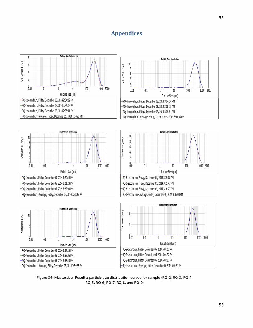
55
55
Appendices
Particle Size Distribution
0.01 0.1 1 10 100 1000 3000
Particle Size (µm)
0
2
4
6
8
Volu
me (%
)
RQ-2-second run, Friday, December 05, 2014 2:34:22 PM
RQ-2-second run, Friday, December 05, 2014 2:35:02 PM
RQ-2-second run, Friday, December 05, 2014 2:35:41 PM
RQ-2-second run - Average, Friday, December 05, 2014 2:34:22 PM
Particle Size Distribution
0.01 0.1 1 10 100 1000 3000
Particle Size (µm)
0
2
4
6
8
10
Volu
me (%
)
RQ-4-second run, Friday, December 05, 2014 3:04:36 PM
RQ-4-second run, Friday, December 05, 2014 3:05:15 PM
RQ-4-second run, Friday, December 05, 2014 3:05:54 PM
RQ-4-second run - Average, Friday, December 05, 2014 3:04:36 PM
Particle Size Distribution
0.01 0.1 1 10 100 1000 3000
Particle Size (µm)
0
2
4
6
8
10
Volu
me (%
)
RQ-5-second run, Friday, December 05, 2014 3:20:49 PM
RQ-5-second run, Friday, December 05, 2014 3:21:28 PM
RQ-5-second run, Friday, December 05, 2014 3:22:08 PM
RQ-5-second run - Average, Friday, December 05, 2014 3:20:49 PM
Particle Size Distribution
0.01 0.1 1 10 100 1000 3000
Particle Size (µm)
0
2
4
6
8
10
Volu
me (%
)
RQ-6-second run, Friday, December 05, 2014 3:35:08 PM
RQ-6-second run, Friday, December 05, 2014 3:35:47 PM
RQ-6-second run, Friday, December 05, 2014 3:36:27 PM
RQ-6-second run - Average, Friday, December 05, 2014 3:35:08 PM
Particle Size Distribution
0.01 0.1 1 10 100 1000 3000
Particle Size (µm)
0
5
10
Volu
me (%
)
RQ-7-second run, Friday, December 05, 2014 3:54:26 PM
RQ-7-second run, Friday, December 05, 2014 3:55:06 PM
RQ-7-second run, Friday, December 05, 2014 3:55:45 PM
RQ-7-second run - Average, Friday, December 05, 2014 3:54:26 PM
Particle Size Distribution
0.01 0.1 1 10 100 1000 3000
Particle Size (µm)
0
5
10
Volu
me (%
)
RQ-9-second run, Friday, December 05, 2014 5:01:53 PM
RQ-9-second run, Friday, December 05, 2014 5:02:32 PM
RQ-9-second run, Friday, December 05, 2014 5:03:11 PM
RQ-9-second run - Average, Friday, December 05, 2014 5:01:53 PM
Figure 34: Mastersizer Results; particle size distribution curves for sample (RQ-2, RQ-3, RQ-4, RQ-5, RQ-6, RQ-7, RQ-8, and RQ-9)

56
56
Particle Size Distribution
0.01 0.1 1 10 100 1000 3000
Particle Size (µm)
0
5
10
Volum
e (%
)
RQ-10-second run, Friday, December 05, 2014 5:18:23 PM
RQ-10-second run, Friday, December 05, 2014 5:19:02 PM
RQ-10-second run, Friday, December 05, 2014 5:19:41 PM
RQ-10-second run - Average, Friday, December 05, 2014 5:18:23 PM
Particle Size Distribution
0.01 0.1 1 10 100 1000 3000
Particle Size (µm)
0
5
10
Volu
me (%
)
RQ-11-second run, Friday, December 05, 2014 5:36:52 PM
RQ-11-second run, Friday, December 05, 2014 5:37:31 PM
RQ-11-second run, Friday, December 05, 2014 5:38:10 PM
RQ-11-second run - Average, Friday, December 05, 2014 5:36:52 PM
Particle Size Distribution
0.01 0.1 1 10 100 1000 3000
Particle Size (µm)
0
5
10
Volu
me (%
)
RQ-14-second run, Friday, December 05, 2014 6:46:15 PM
RQ-14-second run, Friday, December 05, 2014 6:46:54 PM
RQ-14-second run, Friday, December 05, 2014 6:47:33 PM
RQ-14-second run - Average, Friday, December 05, 2014 6:46:15 PM
Particle Size Distribution
0.01 0.1 1 10 100 1000 3000
Particle Size (µm)
0
5
10
Volu
me (%
)
RQ-15-second run, Friday, December 05, 2014 7:07:24 PM
RQ-15-second run - Average, Friday, December 05, 2014 7:07:24 PM
RQ-15-second run, Friday, December 05, 2014 7:08:03 PM
RQ-15-second run, Friday, December 05, 2014 7:08:42 PM
Particle Size Distribution
0.01 0.1 1 10 100 1000 3000
Particle Size (µm)
0
5
10
Volum
e (%
)
RQ-12-second run, Friday, December 05, 2014 6:00:30 PM
RQ-12-second run, Friday, December 05, 2014 6:01:09 PM
RQ-12-second run, Friday, December 05, 2014 6:01:48 PM
RQ-12-second run - Average, Friday, December 05, 2014 6:00:30 PM
Particle Size Distribution
0.01 0.1 1 10 100 1000 3000
Particle Size (µm)
0
5
10 Volu
me (%
)
RQ-13-second run, Friday, December 05, 2014 6:31:43 PM
RQ-13-second run, Friday, December 05, 2014 6:32:22 PM
RQ-13-second run, Friday, December 05, 2014 6:33:01 PM
RQ-13-second run - Average, Friday, December 05, 2014 6:31:43 PM
Figure 35: Mastersizer Results; particle size distribution curves for sample (RQ-10, RQ-11, RQ-12, RQ-13, RQ 14, and RQ-15)

57
57
Figure 36: Mastersizer Results; particle size distribution curves for sample (RQ-17, RQ-18, RQ-19, and RQ-20)
Particle Size Distribution
0.01 0.1 1 10 100 1000 3000
Particle Size (µm)
0
2
4
6
8
Volu
me (%
)
RQ-19-second run, Friday, December 05, 2014 8:09:13 PM
RQ-19-second run, Friday, December 05, 2014 8:09:52 PM
RQ-19-second run, Friday, December 05, 2014 8:10:31 PM
RQ-19-second run - Average, Friday, December 05, 2014 8:09:13 PM
Particle Size Distribution
0.01 0.1 1 10 100 1000 3000
Particle Size (µm)
0
5
10 Volu
me (%
)
RQ-18-second run, Friday, December 05, 2014 7:54:28 PM
RQ-18-second run, Friday, December 05, 2014 7:55:07 PM
RQ-18-second run, Friday, December 05, 2014 7:55:46 PM
RQ-18-second run - Average, Friday, December 05, 2014 7:54:28 PM
Particle Size Distribution
0.01 0.1 1 10 100 1000 3000
Particle Size (µm)
0
2
4
6
8
10
Volu
me (%
)
RQ-17-second run, Friday, December 05, 2014 7:38:20 PM
RQ-17-second run - Average, Friday, December 05, 2014 7:38:20 PM
RQ-17-second run, Friday, December 05, 2014 7:39:39 PM
RQ-17-second run, Friday, December 05, 2014 7:39:00 PM
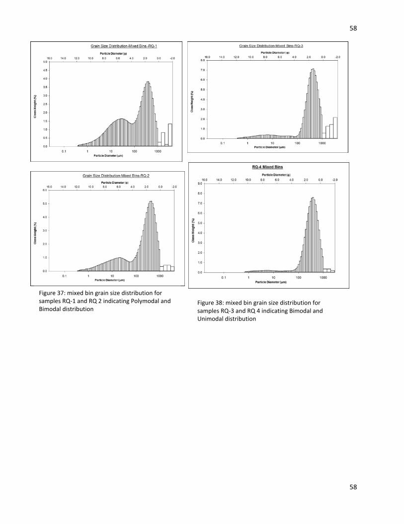
58
58
Figure 37: mixed bin grain size distribution for samples RQ-1 and RQ 2 indicating Polymodal and Bimodal distribution
Figure 38: mixed bin grain size distribution for samples RQ-3 and RQ 4 indicating Bimodal and Unimodal distribution

59
59
Figure 39: mixed bin grain size distribution for samples RQ-5 and RQ 6 indicating Unimodal and Unimodal distribution
Figure 40: mixed bin grain size distribution for samples RQ-7 and RQ 8 indicating Unimodal and Bimodal distribution
Figure 41: mixed bin grain size distribution for Gravelly sand (RQ-9) indicating Unimodal distribution

60
60
Figure43: mixed bin grain size distribution for sand (RQ-10) and gravelly sand (RQ11) indicating Unimodal and Unimodal distribution
Figure 42: mixed bin grain size distribution for samples RQ-12 and RQ 13 indicating Unimodal and Unimodal distribution
Figure 44: mixed bin grain size distribution forRQ-14 (Gravelly sand) indicating Unimodal distribution

61
61
Figure 45: mixed bin grain size distribution for sand (RQ-16) and gravelly sand (RQ 17) indicating Unimodal distribution
Figure 46: mixed bin grain size distribution for sand (RQ-18) and sandy gravel (RQ 19) indicating unimodal and Trimodal distribution

62
62
Sample RQ-1: grain shape analysis results Sample RQ-2: Grain shape analysis results
Sample RQ-3: Grain shape results Sample RQ-4: Grain shape results
Sample RQ-5: Grain shape results Sample RQ-6: Grain shape results
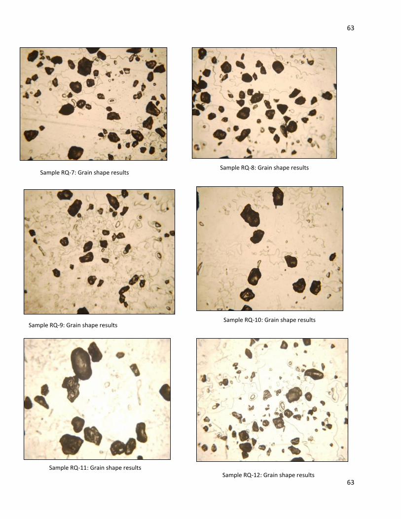
63
63
Sample RQ-8: Grain shape results Sample RQ-7: Grain shape results
Sample RQ-9: Grain shape results
Sample RQ-12: Grain shape results Sample RQ-11: Grain shape results
Sample RQ-10: Grain shape results

64
64
Sample RQ-13: Grain shape results
Sample RQ-15: Grain shape results
Sample RQ-17: Grain shape results Sample RQ-18: Grain shape results
Sample RQ-16: Grain shape results
Sample RQ-14: Grain shape results
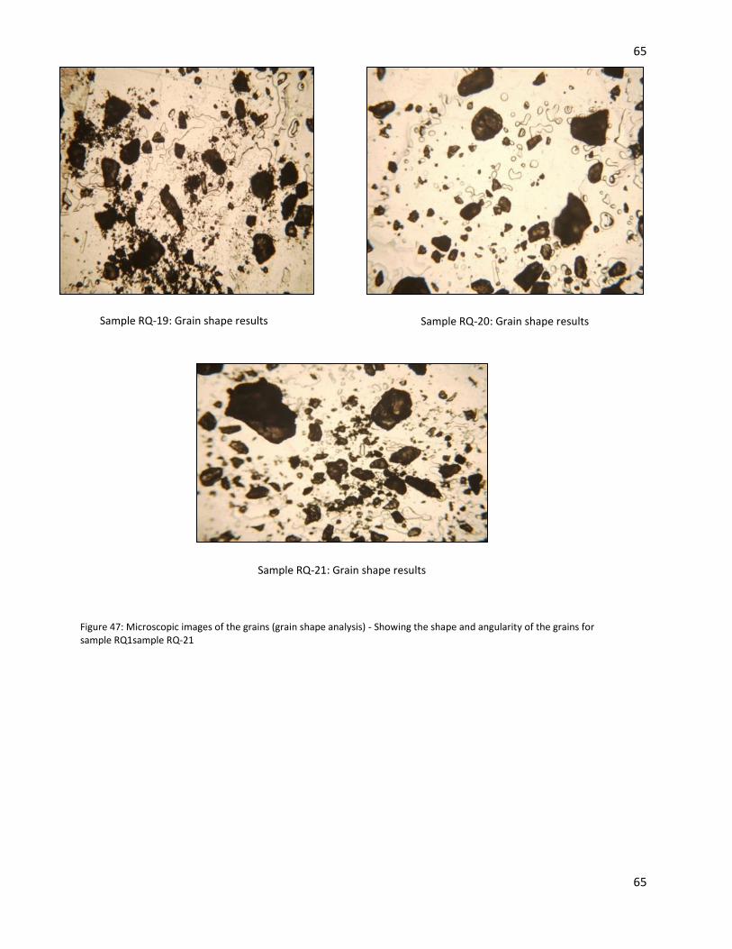
65
65
Sample RQ-20: Grain shape results Sample RQ-19: Grain shape results
Figure 47: Microscopic images of the grains (grain shape analysis) - Showing the shape and angularity of the grains for sample RQ1sample RQ-21
Sample RQ-21: Grain shape results
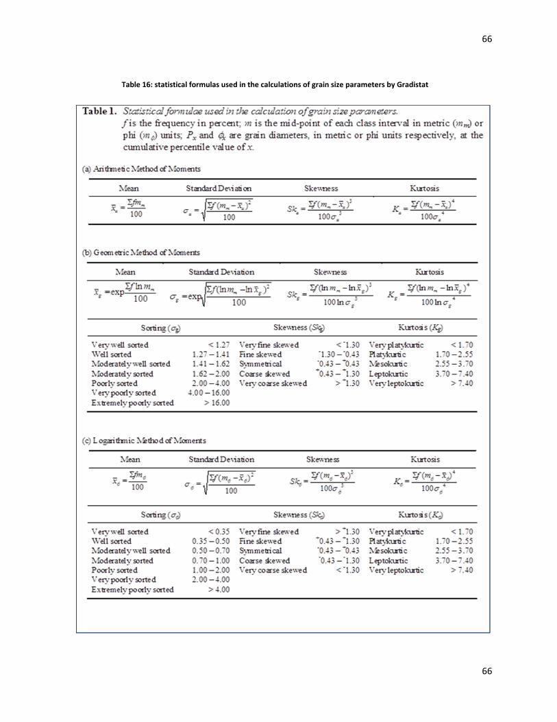
66
66
Table 16: statistical formulas used in the calculations of grain size parameters by Gradistat

67
67
Table 17: Dynamic viscosity values of liquid water used to determine the kinematic viscosity to calculate the hydraulic conductivity

68
68
Figure 48: Grain size distribution –Half phi-Sample RQ-1(polymodal) to RQ-2 (bimodal) indicating a change in resolution hence varying modes.
Figure 49: Grain size distribution –Half phi-Sample RQ-3(Bimodal) to RQ-4 (unimodal) indicating a change in resolution hence varying modes.

69
69
Figure 50: Grain size distribution –Half phi-Sample RQ-5(Unimodal) to RQ-6 (unimodal) indicating a change in resolution hence varying modes.
Figure 51: Grain size distribution –Half phi-Sample RQ-7(Unimodal) to RQ-8 (Bimodal) indicating a change in resolution hence varying modes.

70
70
Figure 52: Grain size distribution –Half phi-Sample RQ-9 (Unimodal) to RQ-10 (Unimodal) indicating a change in resolution hence varying modes.
Figure53: Grain size distribution –Half phi-Sample RQ-11 (Unimodal) to RQ-12 (Unimodal) indicating a change in resolution hence varying modes.
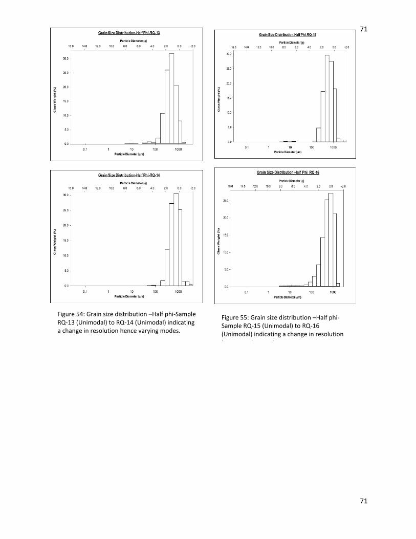
71
71
Figure 54: Grain size distribution –Half phi-Sample RQ-13 (Unimodal) to RQ-14 (Unimodal) indicating a change in resolution hence varying modes.
Figure 55: Grain size distribution –Half phi-Sample RQ-15 (Unimodal) to RQ-16 (Unimodal) indicating a change in resolution hence varying modes.
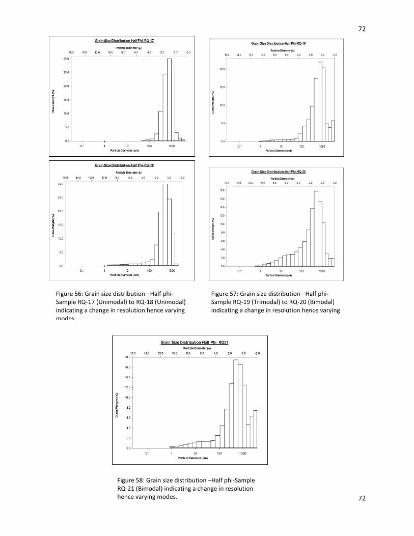
72
72
Figure 56: Grain size distribution –Half phi-Sample RQ-17 (Unimodal) to RQ-18 (Unimodal) indicating a change in resolution hence varying modes.
Figure 57: Grain size distribution –Half phi-Sample RQ-19 (Trimodal) to RQ-20 (Bimodal) indicating a change in resolution hence varying modes.
Figure 58: Grain size distribution –Half phi-Sample RQ-21 (Bimodal) indicating a change in resolution hence varying modes.

73
73
Figure 59: Samples pictures of RQ-1(polymodal loess), RQ 2(bimodal loess), RQ-3(Bimodal gravelly sand) grains examined under the
petrographic microscope to determine the angularity and sphericity.
Figure 60: Samples pictures of RQ-4(Unimodal gravelly sand ) to RQ5 (Unimodal sand) grains examined under the petrographic microscope to determine the angularity and sphericity.

74
74
Figure 61: Samples pictures of RQ-6 (Unimodal gravelly sand) to RQ-7(Unimodal gravelly sand) grains examined under the petrographic microscope to determine the angularity and sphericity.

75
75
Figure 62: Samples pictures of RQ-8 (bimodal gravelly sand) to RQ-9 (Unimodal gravelly sand) grains examined under the petrographic microscope to determine the angularity and sphericity.
Figure 63: Samples pictures of RQ-10 (Unimodal sand) to RQ-11(Unimodal gravelly sand) grains examined under the petrographic microscope to determine the angularity and sphericity.

76
76
Figure 64: Samples pictures of RQ-12 (Unimodal sandy gravel) to RQ-13 (Unimodal sand) grains examined under the petrographic microscope to determine the angularity and sphericity.
Figure 65: Samples pictures of RQ-14 (unimodal gravelly
sand) to RQ-15 (unimodal gravelly sand) grains examined under the petrographic microscope to determine the angularity and sphericity.

77
77
Figure 66: Samples pictures of RQ-16 (unimodal sand) to RQ-17 (unimodal gravelly sand) grains examined under the petrographic microscope to determine the angularity and sphericity.
Figure 67: Samples pictures of RQ-18(unimodal sand) to RQ-19(trimodal sandy gravel) grains examined under the petrographic microscope to determine the angularity and sphericity.

78
78
Figure 68: Samples pictures of RQ-20 (bimodal gravelly muddy sand) to RQ-21 (bimodal muddy sandy gravel) grains examined under the petrographic microscope to determine the angularity and sphericity.
Figure 69 : RQ-1shows poorly sorted Polymodal peblly loess sample,it represents the surface portion of the core
Figure 70: RQ-3 – Bimodal muddy sandy gravel sample showing a poor sorting
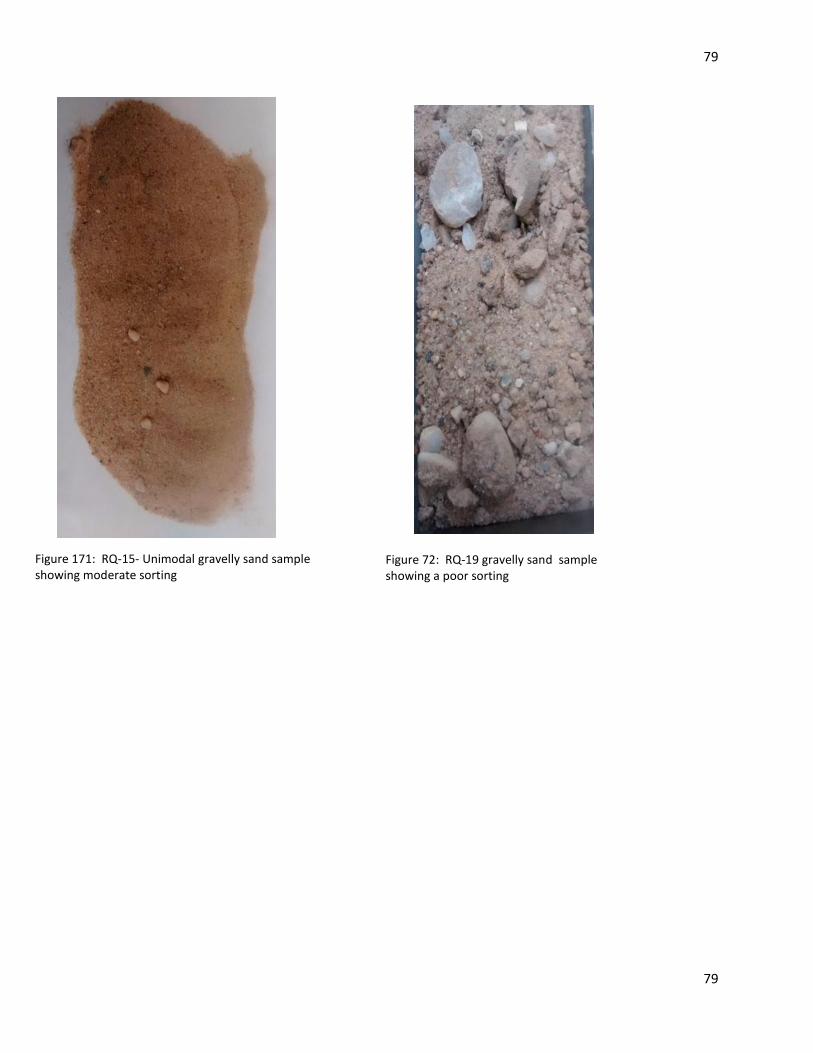
79
79
Figure 171: RQ-15- Unimodal gravelly sand sample showing moderate sorting
Figure 72: RQ-19 gravelly sand sample showing a poor sorting

80
80
Figure 73: RQ-20- A poorly sorted bimodal gravelly Muddy Sand sample at the depth of 32ft below surface.

81
81
Top Related