


Languages
Pages
Legal

Buehler 1
Determinants of Automobile Use A Comparison of Germany and the US
by Ralph Buehler
Virginia Tech University
Ralph Buehler PhD Assistant Professor School of Public and International Affairs Urban Affairs and Planning Program Virginia Tech University 1021 Prince Street Suite 200 Alexandria VA 22314 Email ralphbu[at]vtedu A revised version of this article has been accepted for publication in the Transportation Research Record
Please cite any references to this article as
Ralph Buehler ldquoDeterminants of Automobile Use Comparison of Germany and the USrdquo Transportation Research Record Journal of the Transportation Research Board No 2139 2009 pp 161-171
Buehler 2
Abstract
Germany and the US have among the highest motorization rates in the world Yet Americans make a 40 higher share of their trips by car and annually drive twice as many kilometers per capita as Germans Automobile use is linked to unsustainable trends such as climate change oil dependence traffic fatalities congestion and obesity International differences in car use can be attributed to socioeconomic and demographic factors spatial development patterns transport policies and culture Arguably differences in socio-economic and demographic factors together with denser more compact spatial development patterns and more automobile restrictive transport policies in Germany can help explain less car use there Using two comparable individual level national travel surveys this paper empirically investigates the role of socio-economic and demographic factors spatial development patterns and transport policies in explaining differences in automobile use in Germany and the US
In both countries higher population density a greater mix of land uses household proximity to a transit stop fewer cars per household and higher car operating costs are associated with shorter daily automobile travel distances However considerable differences remain for example Americans in settlements of more than 5000 people per square kilometer drive as many kilometers as Germans in settlements with five times lower density A multivariate analysis shows thatmdashcontrolling for socioeconomic factorsmdashpopulation density and automobile operating costs play a role in explaining differences in travel This is good news for the US since denser more mixed-use developments and more automobile restrictive policies can help increase the sustainability of the transport system In Germany travel behavior is more homogeneous across all groups of society and in all spatial settlement patterns than in the US This is potentially related to historically higher gasoline prices and greater availability of alternative means of transport which provide incentives for walking cycling and transit use
Buehler 3
1 Increasing Motorization in Both Countries But More Sustainable Transportation in Germany Over the last 50 years Germany and the US have displayed similar trends of increasing car
ownership and use In 2006 the US had the highest and Germany the fourth highest car ownership rate in the world (IRF 2007 OECD 2003-2007) Mobility in Germany and the US have developed on two different levels however In 2005 Americans owned 760 cars and light trucks per 10000 population compared to 560 in Germany (BMVBS 1991-2008 FHWA 1990-2008) Moreover Americans drove about 24000 kilometers in a car per year compared to only 11000 kilometers for Germans Even residents in dense US states such as New Jersey drove roughly 60 more kilometers per year than Germans (BTS 2006) In 2001 Americans made 87 of all trips by automobile compared to 61 for Germans This difference also holds for urban areas most German cities have a car modal share of up to 55 compared to roughly 80 for work trips in most US metropolitan areas (FHWA 2003 Socialdata 2006)
Automobile use is at the center of many unsustainable trends such as air pollution due to
tail pipe emissions oil dependence traffic fatalities and injuries traffic congestion urban sprawl loss of open space and obesity due to sedentary life-styles (Pucher amp Lefegravevre 1996 TRB 2001 Vuchic 1999) Dissimilar levels of car use have resulted in differences in the sustainability of the two countriesrsquo transportation systems Even though both countries have mandated the use of advanced technology Germany has been more successful in limiting negative externalities of car usemdashmainly by influencing travel behavior through more automobile restrictive transport policies
First in 2005 there were about half as many traffic deaths per 1000 population in Germany than the US (65 vs 147) (IRTAD 2008) Even adjusting for vehicle kilometers of car travel Germany was safer 78 compared to 90 deaths per one billion vehicle kilometers of car travel in the US (IRTAD 2008) Second the percentage share of obese adults was twice as high in the US as in Germany in 2006 (32 vs 13 of the population over 15 years old) (OECD 2003-2007) Driving less and cycling and walking more could help burn more calories during daily life and reduce obesity Third energy use of automobiles and light trucks is less efficient in the US than in Germany 27 Mega Joules of energy per passenger kilometer in the US compared to 20 Mega Joules for Germany (DOE 2007 ORNL 2008 UBA 2005) Fourth over 30 of all CO2 emissions in the US and about 20 in Germany are caused by the transportation sectors (BMVBS 1991-2008 ORNL 2008) Lastly American households spend roughly 19 of their disposable income on transportation compared to only 14 for Germans This difference is mainly driven by ownership and depreciation costs for multiple cars in US households
The paper proceeds as follows In the next section a literature review identifies four
groups of independent variables as explanatory factors for differences in car use and sustainable transport in Germany and the US Most studies are either descriptive or aggregate level statistical analysis All comparative multivariate studies rely on strong assumptions about the comparability of the data and most focus on socioeconomic factors but fail to include variables describing spatial development patterns and transport policies The data for this analysis originates from two uniquely comparable national travel surveys which were enriched with data capturing spatial development patterns and proxies for transport policy Subsequently descriptive and bi-variate statistics for independent and dependent variables show that for all
Buehler 4
groups of society and at all spatial development patterns Americans are more car dependent than Germans After that a multivariate regression approach for explaining international differences in travel behavior is introduced The analysis finds that spatial development patterns and transport policies play a role in explaining differences in travel behavior even after controlling for socioeconomic and demographic factors
2 Determinants of Car Use in Europe and North America
Only eight descriptive studies which were all published before 1999 explicitly compare
travel behavior in Germany and the US Thus the literature review was expanded to contain international comparative studies of Western European and North American countries in general which were published after 1980 A review of 50 international comparative studies shows that differences and similarities in travel behavior within and across countries are mainly attributed to (1) transport and land-use policies (2) demographic and socioeconomic factors (3) spatial development patterns and (4) cultural preferences (Buehler 2008)
Roughly 70 of the studies reviewed are descriptive 20 are multivariate analysis based on city or country wide averages and only 10 of the studies rely on individual level data Most international comparative studies are plagued by dissimilarity in data and methods or by the aggregate nature of available travel data Generally strong assumptions are made about the comparability of data and travel behavior is compared on the city or country level However individualsmdashnot cities or countriesmdashmake daily travel choices and therefore individual level analysis is most appropriate While most descriptive studies point to the importance of transport policies and spatial development patterns many multivariate studies focus on socioeconomic and demographic factors More recently some individual level studies have emerged that attempt to include spatial development and transport policy variables
Table 1 summarizes major characteristics of individual level comparative studies that
compare European with North-American countries and include measures of urban form The table excludes other descriptive aggregate level and non-international comparative studies Using a sample of 20000 individuals Giuliano and Narayan (Giuliano amp Narayan 2003 2006) estimate linear regression models to measure factors influencing trip distance and trip frequency They find that socio-economic and urban form variables work in the same direction in the US and the UK For example car ownership is positively related to travel distance and number of trips per day Metropolitan size only has a small effect on trip distance and frequency Higher residential densities are associated with shorter trip distances in the US but not in the UK where densities of all settlements were more homogeneous Based on the same data Giuliano and Dargay (Giuliano amp Dargay 2005) employ a structural model to disentangle the connection of land use car ownership and travel They conclude that car ownership is correlated with population density as well as policy variables not directly measured in their modelmdashsuch as the costs of operating and owning a car
Three studies by Axhausen and colleagues (Axhausen et al 2002 Axhausen amp Simma 2001 Simma amp Axhausen 2003) compare transit and car use in Holland Switzerland England Germany and the US Timing methods data and geographic coverage vary across the travel surveys used for the study To overcome these differences the researchers rely on strong assumptions concerning the comparability of their data and results They use Structural Equation Modeling (SEM) to distinguish between direct effects of certain variables on travel and indirect
Buehler 5
effect via other variables The study finds that the connection of socioeconomic factors and travel are stable across countries The only variable related to spatial development patterns is an urban vs rural distinction which yields lower automobile ownership levels in cities compared to rural areas Transit season ticket ownership a variable measuring policy is related to more transit use
Timmermanns and colleagues (Timmermanns et al 2003) compare the relationship of urban spatial development patterns access to transit and travel behavior across five regions in five different countries None of their spatial context variables are significant in explaining differences in travel behavior Even though not part of their analysis they conclude that within a society ldquopsychological principlesrdquo seem to be more important in explaining travel behavior than measurable characteristics included in their analysis
Overall socioeconomic and demographic factors have been well established as
explanatory factors for international differences in travel behavior in the literature Empirical evidence for the connection of spatial development patterns and travel in international comparative studies is less clear These variables are very often omitted from multivariate models or when included result in mixed inconsistent or unexpected results Especially the limited comparability of data can drive the results Transport and land-use policies are mentioned in most studies of travel behavior but rarely explicitly tested in individual level international comparative multivariate studies Cultural differences are difficult to measure but many authors allude to cultural differences in shaping spatial development policies and travel This study tries to overcome some of these shortcomings and can help to shed more light on the role of socio-economic and demographic factors spatial development patterns and policies in determining travel behavior
Two Uniquely Comparable National Travel Surveys
Two national travel surveys the National Household Travel Survey 2001 (NHTS) for the US and the Mobility in Germany 2002 (MiD) are the main data sources for this comparison Both surveys are based on similar data collection methods and contain comparable variables Similarities and differences of the two surveys are summarized in Table 2 Cells shaded in grey indicate comparability between the two surveys cells in white display remaining differences These two surveys are the most comparable national travel surveys that currently exist The data allow a detailed investigation of the role of socioeconomic factors spatial development patterns and policies to explain similarities and differences of individual travel behavior Some variables for the analysis were readily available for comparison Several other variables had to be added to the datasets and others had to be transformed or generated for the purpose of this comparison The next section introduces a general model for explaining international differences in travel behavior
TABLES 1 AND 2 ABOUT HERE
3 A Multivariate Approach For Comparing International Differences in Automobile
Use Car use is at the center of many unsustainable trends described above Variability in car
use within and across countries can be explained by dissimilarities in socioeconomic and
Buehler 6
demographic variables spatial development patterns transportation policies and cultural preferences Equation 1 summarizes these factors in a general model for comparing similarities and differences in travel behavior
[Equation (1) TB=f (SE SD TP CP)]
TB=travel behavior SE=socioeconomics and demographics SD=spatial development patterns TP= transportation policies CP=cultural preferences
These explanatory factors might have a different impact in each country contributing to a
unique transportation system This analysis (1) explores differences and similarities in car use within and between the countries and (2) evaluates the contribution of explanatory factors to explained variability within countries The models are based on a pooled sample of 87635 individuals from Germany and the US The following sections briefly summarize general differences in transport policy spatial development patterns and socioeconomics between the countries The focus is however on a description of policy differences the introduction of proxy variables to measure policy differences and variables measuring land use Tables 3 and 4 describe the variables in the analysis in more detail (including socio-economic and demographic factors) and list level of measurement descriptive statistics and data sources
Transport Policies
Policies and institutions in the US contribute to making car use cheaper easier and more common than in Germany In contrast to Germany all levels of government in the US have prioritized funding for highways over all other modes of transportation In 2005 for example revenues from roadway user taxes and fees in Germany were 26 times larger than roadway expenditures by all levels of government compared to net subsidies for roadways in the US (BMVBS 1991-2008 FHWA 1990-2008) The retail price of gasoline is about twice as high in Germany than the US Roughly 65 of the gasoline retail price in Germany is taxes compared to only 15 in the US (EIA 2008 IEA 2008) Moreover since the 1960s most German municipalities promote non-automobile travel and impose restrictions on driving thus making car travel in cities slower and less attractive (Hass-Klau 1993 Pucher amp Buehler 2008 Pucher amp Lefegravevre 1996) In 2002 average car travel speeds in the US were 25 percent faster than in Germany (41 vs 33 kmh) Moreover Germany has a longer history of subsidies for transit walking and cycling which has helped making those modes of transport a feasible alternative to the car Even though total subsidies for transit are higher in Germany the use of government funds is more efficient there In 2002 for example government subsidies comprised 35 percent of the operating budgets for public transit systems in Germany but a full 60 percent of public transit operating budgets in the US (APTA 2006 Roumlnnau 2004 Roumlnnau Schallaboumlck Wolf amp Huumlsing 2002 VDV 2005)
It is difficult to include policy variables in individual level multivariate analysis In this
analysis policy differences towards the automobile in Germany and the US are captured with proxy variables measuring (1) automobile operating costs and (2) household distance from a transit stop Car operating costs per kilometer are added to the datasets based on type of automobile fuel efficiency and prices assuming a 55 share of urban travel In 2001 average automobile operating costs were US 42 cents in America and 95 cents in Germany Two nominal variables capture access to transit by comparing households within 400m and 400-
Buehler 7
1000m from a transit stop to households more than 1000m away In the US 31 of households lived within 400m of transit compared to 53 in Germanymdashthus capturing the more homogeneous distribution of transit service there compared to the US
TABLES 3 amp 4 ABOUT HERE
Spatial Development Patterns Over the last 50 years Germany and the US both experienced increasing suburbanization
and decreasing population densities However the density of German settlements is two and a half to three times greater than that of their US counterparts (Kenworthy amp Laube 2001) The difference in settlement densities of inner and outer suburbs between Germany and the US are particularly pronounced (Buehler 2008 Kenworthy amp Laube 2001 Stein Wolf amp Hesse 2005)
In Germany land-use policies are much stricter than in the US making new developments outside of already built-up areas difficult allowing more mixed use and thus limiting urban sprawl (Buehler 2008 Hirt 2007 Schmidt amp Buehler 2007) Moreover the German spatial planning system prescribes coordination of transportation planning and land-use planning (BMVBS 2008 Koumlhler 1995 TRB 2001) Local regional and state spatial plans have to take transportation plans into account and vice versa This integration of planning potentially allows aligning planning goals and minimizes adverse impacts
For this analysis population density and mix of residences and workplaces were added to
the datasets and capture differences in spatial development patterns In this particular sample population densities in Germanymdashmeasured as population over built-up areamdashare two and a half times higher than in the US The distribution of the population density variable for Germany is much more homogeneous than that for the US where densities vary from the rural Mid-West to downtown Manhattan NY Mix of land uses is measured as a variable ranging from zero to one A value of one indicates a balanced mix of households and work places while a zero stands for almost no mix of work and residential uses The mean of both countriesrsquo distributions are relatively close together (031 vs 034) This is unexpected as Germany is thought to have more mixed-use than the US (Hirt 2007) A closer look reveals that the German distribution is more homogeneous than the US distribution The US median for mix of uses was 22 lower than the mean and 30 lower than the median for Germany Moreover this quantitative measure does not capture the quality of the mix of use There is no information available that would show if skill levels of residents match with jobs available in the area This additional information would be useful but was not available from the enriched datasets
Bivariate analysis shows that higher population density and a greater land use integration
of workplaces and housing reduce car use in both countries However Americans in any spatial setting are more car-dependent than Germans For example at any population density category Americans drive between 60 and 80 more kilometers per day (Figure 1) Americans who live in the highest population density category at over 5000 people per km2 only drive slightly fewer km per day than Germans in the lowest population density category at less than 1000 people per km2 Similarly Americans living in areas with a high mix of residences and workplaces drive more kilometers per day than Germans in areas with less mix Some readers might assume that trip distance could help explain the difference in car use Indeed in Germany 34 of all trips were shorter than one mile and 54 of trips were shorter than two miles compared to only 27
Buehler 8
(lt1 mile) and 39 (lt2 miles) in the US But in the US 67 of trips shorter than one mile and 90 of trips shorter than 2 miles were made by car compared to 27 and 61 in Germany
FIGURE 1 ABOUT HERE
Socioeconomic and Demographic Factors
Variables controlling for socioeconomic and demographic factors are household income cars per household driver age gender family life cycle status and an indicator if the respondent has a driverrsquos license Bivariate analysis finds that in both countries higher incomes more cars per household driver and employment are related to more car travel For all variables analyzed here however Americans are far more car-dependent than Germans In many cases the most car-dependent group of society in Germany uses the automobile less than the least car-oriented group in the US For example higher income households drive more than poorer households however households in the highest German income quartile drive fewer kilometers than American households in the lowest income quartile
4 Results of the Models
Results of two sets of models are presented in Table 5 Both sets are based on a pooled
sample including Germans and Americans The first set of models investigates the importance of socioeconomic and demographic variables spatial development patterns and transport policies in explaining differences in travel behavior in the pooled sample The second set uses interaction effects for Germany to determine the sign magnitude and statistical significance of differences in coefficients between the two countries Details of the two models are introduced in the respective sections below
Combined Models For the first three models groups of independent variables are entered one after the other
All variables measuring spatial development patterns and proxies for transport policies are included in Model 1 Socioeconomic and demographic factors are added in Model 2 and the country dummy variable is added in Model 3 This allows controlling for changes in total variability explained (adjusted R2) for different groups of independent variables Proxies for transport policies and spatial development patterns reach an adjusted R2 of 010 Once socioeconomic and demographic factors are included the adjusted R2 increases to 017 Adding the country dummy does not significantly increase the percentage of variability explained This method also identifies omitted variables bias through changing signs and magnitudes of coefficients across the different models For example the coefficient for operating cost per kilometer of car use drops significantly once the country dummy variable is includedmdashindicating that the cost variable had picked-up other differences between Germany and the US in Models 1 and 2
The sequence of entering the variable groups is chosen based on theoretical interest and novelty of independent variables for multivariate international comparative research This approach has one weakness however the order of entering groups of variables influences changes in adjusted R2 In order to identify the unique contribution of each group of independent variables three separate models are additionally estimated each with just one group of
Buehler 9
independent variables The results are as follows adjusted R2 is 012 for a model with socioeconomic and demographic variables alone 010 for spatial development patterns and policy proxy variables alone and 007 for the dummy variable alone Moreover the groups of independent variables were entered in all possible sequences to control for differences in adjusted R2 due to the order of entering the variables Comparing adjusted R2 for the full reduced and individual models allows interpreting the magnitude of variability explained by each group of variable independently Socioeconomic and demographic variables explain between seven to 12 of total variability in travel behavior Transportation policies and spatial development patterns explain between three and ten percent of the variability in the data The dummy variable captures between one and seven percent of the variability Overall adjusted R2
reaches 17mdashwhich might seem low to some readers but is common for models with individual level travel survey data
F-statistics for all models indicate that the independent variables had joint statistical
significance in explaining the dependent variable The standard tests for multicoliniarity (Variance Inflation Factor Tolerance and Condition Index) yielded satisfactory results The overall VIF was 223 well below the suggested the critical value of 5 The smallest tolerance value was 02 double the suggested critical value of 01 Another test the condition index confirms these results Robust coefficients and errors were estimated to control for potential spatial autocorrelation Interaction Effects to Capture Country Specific Differences
Coefficients of the independent variables for Models 1-3 all point in the theoretically expected direction but hide differences in sign magnitude and statistical significance within each country Therefore a second set of models is estimated to capture differences between the countries Here for every independent variable one additional interaction variable for Germany is included in the analysis Equation 2 displays a general model for explaining international similarities and differences in travel behavior with interaction effects
[Equation (2) TB=f (SE SE(G) SD SD(G) TP TP(G) CP)]
Definitions as above (G)=interaction effect for Germany
The coefficients of the independent variables are evaluated according to three criteria (1) sign (2) magnitude (3) and statistical significance First the signs of the coefficients show if theories of travel demand hold true in both countries If so signs of coefficients should point in the same and expected direction in both countries Second the magnitude of the coefficients is expected to vary between the countries Third the statistical difference of coefficients in Germany and the US indicates dissimilarities in travel behavior and transport system
Results of the OLS model with interaction variables are presented in the last two columns
of Table 5 Models with interaction effects are somewhat difficult to interpret since the interaction effect has to be added to the main effect of the variable To avoid confusion and for the convenience of the reader the interaction coefficients of the OLS regression have already been added and can be read-off the table directly
One joint coefficient for both countries indicates coefficients that were not statistically different between the countries Two different coefficientsmdashone for each countrymdashindicate
Buehler 10
statistically significantly different effects in Germany and the US For example Living within 400m of a transit stop reduces daily car travel distance by 65km in the US but only by 32km in Germany Differences in car travel distance between individuals living close and farther away from a transit stop are less pronounced in Germany than in the US Traditionally high gas prices and more possibilities for walking and cycling might encourage Germans at all distances from transit to economize their driving
Moreover a one cent increase in the operating cost per km of car use leads to a 24km
reduction in car kilometers traveled in the US compared to 03km in Germany The magnitude of these coefficients is unexpected as theory would suggest a more elastic demand in Germany given higher gasoline prices better accessibility without a car and greater availability of other modes of transportation there On the other hand it is possible that traditionally higher gas prices in Germany have led to economizing of driving Thus changes in the gas price will have a smaller effect on driving in Germany than in the US where cheap gasoline encourages more trips by car
Furthermore a 1000 people per km2 increase in population density reduces daily car
travel distance by 27km in the US and 18km in Germany Similar to transit access the difference in daily travel distance between low and high density areas is less pronounced in Germany than in the US Again Germans might economize their driving at all population densities Mix of land uses has a similar impact in both countries however
One additional automobile per household driver increases total daily car travel distance by 30km in the US and by 101km in Germany Thus car-ownership has a stronger impact on daily automobile travel distance in Germany The majority of US households own multiple cars (60) Thus most household members have easy access to a car when they need one In Germany the majority of households only own one car (53) thus forcing household members to use other modes of transport once the car is taken by another household member The dummy variable for Germany indicates that Germans drive 377 fewer kilometers per day than Americans
TABLE 5 ABOUT HERE
Improvements for Future Analysis
The unique comparability of the German MiD and the US NHTS surveys constitutes an unprecedented opportunity for individual level international comparisons However some recommendations for improvements of future travel surveys and analyses can be made Most suggestions pertain to (1) better and more comparable data about policies the built environment and personal preferences and (2) more comparable time series data
First cross-sectional data are useful in providing a glimpse into differences in travel in both countries at one point in time However to capture the impacts of variables like gasoline prices transit access income car access or population density observations would have to be measured over timemdashideally by a panel study
Second endogeneity and self-selection bias are always problems for analyses of travel behavior Endogeneity bias can occur (1) if independent variables are also a function of the dependent variable or (2) if independent variables are correlated with omitted variables (Cao Mokhtarian amp Handy 2006) Some researchers argue that the choice of household location and
Buehler 11
car ownership is associated with travel preferences and attitudes Not including specific variables about attitudes and travel preferences could also lead to biased coefficients Several solutions exist to address these problems such as statistical control instrumental variable sample selection models or joint models (Cao et al 2006) All of these approaches come with stringent requirements for comparability of variables and measurements in both countries and are hard to implement with just two cross-sectional surveys
Lastly more and better variables capturing transport policies could improve the analysis For example information about transit supply at different transit stops car parking availability and cost length of bike networks speed limits and road supply could be connected to the two travel surveys Unfortunately this data or geographic identifiers did not exist at a disaggregate level for both countries
5 Conclusion
Two enriched individual level national travel surveys the NHTS for the US and the MiD
for Germany provide a unique opportunity to compare differences in car use between the countries The multivariate analysis shows thatmdasheven after controlling for socioeconomic and demographic factorsmdashspatial development patterns and transport policies play a role in explaining international differences in travel behavior This is good news for transportation policy makers and planners in the US since denser more mixed use developments and more automobile restrictive policies can help increase the sustainability of the transport system If differences were solely driven by socioeconomic factors fewer policy levers would be available to affect changes in travel behavior
Transportation and economic theory would suggest that people with similar social and
economic attributes in Germany and the US should display similar travel behavior For example households with higher incomes are expected to own more cars and to drive more or households in denser areas are predicted to drive less often and for fewer kilometers The analysis shows that these theoretical expectations hold true within each country but they do not hold true across countries Similar people in both countries do not have identical travel behavior For some distributions of socioeconomic and demographic and spatial development variables car use in the two countries does not even overlap For example the highest income quartile in Germany travels less by car than the lowest income quartile in the US And Americans in the highest population density categories drive more kilometers by car than Germans in the lowest density category In the US all groups of society are more reliant on the automobile than their German counterparts Theories in travel behavior are correct but they must consider other contextual factors that influence travel behavior
These contextual factors include transportation policies The analysis shows that all groups
of society in all spatial settlement patterns in Germany drive less than Americans This may be related to historically higher gasoline prices and greater availability of alternative means of transport which has lead Germans to diversify and economize their travel behavior already Spiking gasoline prices and declining vehicle miles of car travel in the summer of 2008 might have been a first indicator for economizing of driving in America Combined with increased availability of transit service and better accessibility via walking and cycling facilities
Buehler 12
Americans might be able to reduce care use and increase the sustainability of their transport system
Buehler 13
6 References
ADAC (2007) Autokosten 2007 Retrieved 0814 2008 from wwwadacde APTA (2006) Transportation Factbook Washington DC Axhausen K W Lleras G C Simma A Ben-Akiva M E Schafer A amp Furutani T (2002)
Fundamental relationships specifying travel behavior - an international travel survey comparison Paper presented at the Transportation Research Board Annual Conference Washington DC
Axhausen K W amp Simma A (2001) Structures of commitment in mode use a comparison of Switzerland Germany and Great Britain Transport Policy 8
BMVBS (1991-2008) Verkehr in Zahlen German transport in figures Berlin German Federal Ministry of Transportation and Urban Development
BMVBS (2004) Mobilitaet in Deutschland - Mobility in Germany Survey Bonn German Federal Ministry of Transportation and Urban Development
BMVBS (2008) Rueckblick Staedtebau und Stadtentwicklung im Wandel - Changes in Urban Planning and Development Bonn German Federal Ministry of Transportation and Urban Development BBR
BTS (2006) State transportation profiles Washington DC Bureau of Transportation Statistics FHWA Buehler R (2008) Transport Policies Travel Behavior and Sustainability A Comparison of Germany and
the US Rutgers University Cao X Mokhtarian P L amp Handy S (2006) Examining the Impacts of Residential Self-Selection on
Travel Behavior Methodologies and Empirical Findings University of California Institute of Transportation Studies
DESTATIS (2005) Statistik Lokal 2003 Wiesbaden Destatis German Federal Office for Statistics DIW (2004) Mobilitaet in Deutschland 2002 Kontinuierliche Erhebung zum Verkehrsverhalten
Endbericht Berlin DIW German Institute for Economic Research DOE (2007) Transportation Energy Intensity Indicators Washington DC Department of Energy EIA (2008) Weekly International Gasoline Prices FHWA (1990-2008) Highway Statistics Retrieved various dates from Federal Highway Administration
FHWA httpwwwfhwadotgovpolicyohim FHWA (2003) Transportation to Work Washington DC Federal Highway Administration German Federal Agency for Employment (2006) Sozialversicherungspflichtige Beschaeftigte am
Arbeitsort Giuliano G amp Dargay J (2005) Car ownership travel and land use a comparison of the US and Great
Britain Transportation Research Part A 40 106-124 Giuliano G amp Narayan D (2003) Another look at travel patterns and urban form The US and Great
Britain Urban Studies 40(11) Giuliano G amp Narayan D (2006) Land use planning as an ingredient of transport policy is there a
sufficient link Paper presented at the Stella Focus Group Meeting Santa Barbara Hass-Klau C (1993) The pedestrian and city traffic New York Belhaven Press Hirt S (2007) The Devil is in the Definitions Contrasting American and German Approaches to Zoning
Journal of the American Planning Association 73(4) 436 - 450 IEA (2008) Energy prices and taxes New York International Energy Agency IRF (2007) World Road Statistics Brussels International Road Federation IRTAD (2008) Selected Risk Values for the Year 2005 Retrieved 01152008 2008 from
httpcemtorgIRTADIRTADPublicwe2html Kenworthy P amp Laube F (2001) Millennium cities database Brussels Belgium UITP
Buehler 14
Koumlhler U (1995) Traffic and transport planning in German cities Transportation Research Part A 29A(4)
Kunert U Kloas J amp Kuhfeld H (2002) Design Characteristics of National Travel Surveys Internationals Comparison for 10 countries Transportation Research Record 1804
OECD (2003-2007) OECD Statistics Paris France Organization of Economic Cooperation and Development
ORNL (2005) National household travel survey 2001 Version 2004 Retrieved 01082005 from Oak Ridge National LaboratoriesFHWA httpnhtsornlgov
ORNL (2008) Transportation Energy Data Book Oak Ridge Oak Ridge National Laboratories Pucher J amp Buehler R (2008) Making Cycling Irresistible Lessons from the Netherlands Denmark and
Germany Transport Reviews 28(1) Pucher J amp Lefegravevre C (1996) The urban transport crisis in Europe and North America Basingstoke
Macmillan Roumlnnau H J (2004) Anforderungen and die Verkehrsfinanzierung - Strategien fuer neue
Organisationsstrukturen und Finanzierungsinstrumente im OumlV Paper presented at the SRL Halbjahrestagung
Roumlnnau H J Schallaboumlck K-O Wolf R amp Huumlsing M (2002) Finanzierung des oeffentlichen Nahverkehrs Politische und wirtschaftliche Verantwortung trennen Der Staedtetag 12
Schmidt S amp Buehler R (2007) The Planning Process in the US and Germany A Comparative Analysis International Planning Studies 12(1) 55-75
Simma A amp Axhausen K W (2003) Commitments and modal usage An analysis of German and Dutch panels Transportation Research Record
Socialdata (2006) Mobility indicators of German cities Retrieved 06122006 from Socialdata wwwsocialdatade
Stein A Wolf U amp Hesse M (2005) Mobilitaet im suburbanen Raum Teil C Regionale Fallstudien Berlin BMVBW
Timmermanns H van der Waerden P Alves M Polak J Ellis S Harvey A S et al (2003) Spatial context and the complexity of daily travel patterns An international comparison Journal of Transport Geography 11
TRB (2001) Making transit work Insight from Western Europe Canada and the United States Washington DC Transportation Research Board National Research Council National Academy Press
US Census Bureau (2006a) Census transportation planning package Workers by place of work and census tract Retrieved 01102006 from FHWA
US Census Bureau (2006b) US Gazetteer files 2000 and 1990 Retrieved 01102006 2006 from httpwwwcensusgovgeowwwgazetteergazettehtml
UBA (2005) Vergleich Der Schadstoffemissionen Einzelner Verkehrstraeger - Comparison of Emissions of Different Modes of Transport Dessau Umweltbundesamt
VDV (2005) VDV Statistik 2005 Retrieved 10122006 2006 from wwwvdvde Vuchic V (1999) Transportation for livable cities New Brunswick NJ Center for Urban Policy Research
(CUPR)
Buehler 15
List of Tables and Figures Table 1 International Comparative Multivariate Statistical Analyses of Travel Behavior in Western Europe and North America with Individual Level Data (Note national studies and comparative studies with aggregate data are excluded from this specific table) (Axhausen et al 2002 Axhausen amp Simma 2001 Giuliano amp Dargay 2005 Giuliano amp Narayan 2003 2006 Simma amp Axhausen 2003 Timmermanns et al 2003) Table 2 Potential Sources of Divergence in National Travel Surveys and Comparability of MID and NHTS (BMVBS 2004 DIW 2004 Kunert Kloas amp Kuhfeld 2002 ORNL 2005) Table 3 Variables in the Regression Analysis Measurement Explanation and Data Sources (ADAC 2007 BMVBS 2004 DESTATIS 2005 German Federal Agency for Employment 2006 ORNL 2005 US Census Bureau 2006a 2006b) Table 4 Descriptive Statistics of Dependent and Independent Variables Table 5 Results of Multivariate Regression Analysis (Dependent Variable = Daily Car Travel Distance) Figure 1 Population Density and Daily Car Travel Distance in Germany and the US
Buehler 16
Socio-economic and Demographic Factors Policy Culture
na 1994 (CH) 1999 (UK) 1994-98 (GER)
Year of Publication Dependent Variables Year of Data Collection
and Countries IncludedAuthor(s)
SimmaAxhausen et al 2001
trips per day by cartransit miles
traveled by cartransit
sex age employment status car availability of children urbanrural indicator transit season
ticket dummy
na1994 (US) 1993 (J) 1992
(CA) 1994 (UK) 1997 (NL)
Axhausen et al na 1994 (A CH) 1995 (US) 1996-98 (UK)
Timmermanns et al 2003 trips tours per day transport mode income HH
size
urbansuburban indicator transit access
indicatorna
2002cars per adults per HH daily trips daily travel
time
workernot worker dummy HH size sex urbanrural indicator na
dummy variable 1995 (US) 199597 (UK)
SimmaAxhausen 2003 car or transit trips per day
sex age employment status HH size car availability transit
season ticket owner drivers license dummy
urbanrural dummy na na 1994-1998 (GER) 198489 (NL)
GiulianoNarayan 2003 trips per day miles of travel per day
sex age employment status income
residential density MSA size na
descriptive car ownership and operating costs
dummy variable 1995 (US) 199597 (UK)
descriptive gas price tax housing
policy
dummy variable
GiulianoDargay 2005 car ownership miles traveled
sex age employment status HH size income lifecycle HH
cars per HH
residential density MSA size distance to transit
houseapartment
Explanatory VariablesSpatial Development
PatternsUrban FormLand Use
GiulianoNarayan 2006 trips per day miles of travel per day
sex age income employment status car ownership
cardriver per HH ratio
MSA size population density 1995 (US) 199597 (UK)
Table 1 International Comparative Multivariate Statistical Analyses of Travel Behavior in Western Europe and North America with Individual Level Data (Note national studies and comparative studies with aggregate data are excluded from this specific table) (Axhausen et al 2002 Axhausen amp Simma 2001 Giuliano amp Dargay 2005 Giuliano amp Narayan 2003 2006 Simma amp Axhausen 2003 Timmermanns et al 2003)
Buehler 17
Range of NTS MiD (Germany) NHTS (US)Survey Period 10 weeks to 14 months 14 months (1101 - 1202) 14 months (0301 - 0402)Collection Rhythm annually to irregularly 76 82 89 02 69 77 83 90 95 01
25848 HH 26082 HH61729 individuals 60228 individuals
167851 trips 248512 trips
Survey Methodphone person mail
Computer Assisted Telephone Interview (95 other 5 paper
based)
Computer Assisted Telephone Interview (100)
Target Population generally civilian population
civilian civilian
Eligibility of HH Members adults children age caps adults and children adults and children
Sampling Technique RDD population registry or other lists
stratified random sample from population register
list assisted random digit dialing
Survey Period 1 to 7 days 1 day travel diary 1 day travel diaryResponse Rates often below 40 of HH 42 of HH 41 of HH
Nonresponse Treatment varies widely collection of HH data collection of HH data
Data Level HH person trip or car HH person trip car HH person trip car
Representativeness Country regions states and other subsections Germany States US Census Regions
Add-ons Yes Yes
Weights vary widelyselection reciprocal non-response
HH size weekday month regional characteristics
selection reciprocal non-response HH size weekday month regional
characteristics
Sample Size 3000 to 63000 HH
Inclusion Criteria vary widely HH where at least 50 of HH members responded HH where at least 50 of HH
members over 18 years old responded
Table 2 Potential Sources of Divergence in National Travel Surveys and Comparability of MID and NHTS (BMVBS 2004 DIW 2004 Kunert et al 2002 ORNL 2005)
Buehler 18
Variable Source
NHTSDESTATIS
CTPP GazetteerDESTATIS BAA
NHTSMiD NHTSMiD NHTSMiD NHTSMiD NHTSMiD
NHTS
MiD
NHTSMiD Germany - US dummy nominal variable value of 1 if respondent is from German sample
Gender nominal variable US value of 1 for male respondentsGermany value of 1 for male respondents
Household lifecycle and employment
series of nominal variables indicating household life cycle and respondents employment status including employed in single HH unemployed in single HH
employed in adult only HH unemployed in adult only HH employed in HH with small children
unemployed in HH with small children employed in HH with older children unemployed in HH with
older children retired in HH of retired individuals
US employed individual in hh with older children as reference category
Germany employed individual in hh with older children as reference category
Car access ratio US ratio of vehicles per household to household members with a drivers licenseGermany ratio of vehicles per household to household members with a drivers license
Teenagerchild nominal variable US value of 1 for individuals younger than driving ageGermany value of 1 for individuals younger than driving age
Household income US dollars US annual income before taxesGermany annual income before taxes
Drivers license nominal variable US value of 1 indicates individual with drivers licenseGermany value of 1 indicates individual with drivers license
Population density population per square kilometer US population per land area on census tractGermany population per settled land area per municipality
Mix of land uses index ranging from 0 (no mix) to 1 (great mix) US index based on ratio of workplaces and residentsGermany index based on ratio of workplaces and residents
Automobile operating cost US cents per kilometer
US operating cost based on type and fuel economy of vehicle (assuming 55 urban) and average state gasoline prices
EPA
Germany operating cost based on type and fuel economy of vehicle (assuming 55 urban) and average gasoline and diesel prices
ADAC
Measurement Explanation
Household distance to a transit stoptwo nominal variables indicating if a household is
located (1) within 400 meters or (2) between 400 and 1000 meters from transit
US distance of a household from a rail station or bus corridor ORNL
Germany distance of a household from a bus stop or a rail station MiD
Table 3 Variables in the Regression Analysis Measurement Explanation and Data Sources (ADAC 2007 BMVBS 2004 DESTATIS 2005 German Federal Agency for Employment 2006 ORNL 2005 US Census Bureau 2006a 2006b)
Buehler 19
Level of Measurement Overall Mean Min Max Mean
GermanyMean US
Overall N
238 485 na
Correlation with Dependent VariableDependent variable
Car travel distance (km) interval ratio 368 0 200 87635
Independent variables
Polic
y
Transit access lt400mnominaldummy
(1= hh within 400m of transit stop)
na 0 1 na na 87399
42 87635
-010
Transit access 400-1000mnominaldummy
(1= hh within 400-1000m of transit stop)
na 0 1 na na 87399 -006
Population density (pop per sqkm) interval ratio 1732 01 9979 2495
-018Automobile operating cost per km in US cents
interval ratio 680 13 191 95
1038 86810 -015
015
Drivers licensenominaldummy
(1=respondent has drivers license)
Mix of use interval ratio 033 001 999 034 031
na 87549 014
86790 -004
Soci
oeco
nom
ic a
nd d
emog
raph
ic v
aria
bles
Household income in US $ interval ratio 54738 2500 115000 49866 59819
Spat
ial
deve
lopm
ent
patt
erns
84529 008
Car accessavailability per HH driver interval ratio 091 0166 4
Younger than 1618nominaldummy
(1=respondent younger than 1618)
na
074 115 87616
87552 -001
0 1 na
na 0 1 na
87551 002
na 87550 -012
Employed in single HH nominaldummy
(1=respondent with job in single HH)
na 0 1 na na
Employed in adult only HHnominaldummy
(1=respondent with job in 2 pers HH)
na 0 1 na na
Unemployed in single HH nominaldummy
(1=respondent without job in single HH)
na 0 1 na na
87553 008
na 87554 -004
Employed in HH with small children
nominaldummy (1=respondent with job in
HH with child 0-5)na 0 1 na na
Unemployed in adult only HHnominaldummy
(1=respondent without job in 2 pers HH)
na 0 1 na
87555 006
Unemployed in HH with small children
nominaldummy (1=respondent without job
in HH with child 0-5)na 0 1 na na 87556 -004
Unemployed in HH with school children
nominaldummy (1=respondent without job in HH with child 6-1618)
na 0 1 na na 87557 -008
na 87558 -002
Sex (Male=1) nominaldummy (1=male) na 0 1 na na
Retired HHnominaldummy
(1=respondent retired in retired HH)
na 0 1 na
87635 -020
87559 005
Germany(10)nominaldummy
(1=Respondent from German sample)
na 0 1 na na
Table 4 Descriptive Statistics of Dependent and Independent Variables
Buehler 20
Model 1 Model 2 Model 3
US Germany
6834 4931 4572(12600) (4662) (4317)
-756 -681 -595 -652 -322(1610) (1447) (1260) (926) (338)
-651 -601 -459 -527 -227(1263) (1166) (877) (588) (264)
-2738 -2278 -0878 -240 -032(4254) (3325) (779) (985) (715)
-270 -250 -224 -273 -178(1936) (1757) (1581) (1115) (320)
-1118 -1129 -1153(1261) (1267) (1296)
008 007(1115) (992)
574 467 301 1007(1274) (1031) (544) (776)
1059 1069(2062) (2098)
-1183 -1203 -1587 -790(1924) (1967) (1507) (637)
157 118 -174 354(180) (135) (149) (299)-389 -443(177) (201)077 038 -126 180
(141) (069) (155) (280)-735 -711
(1066) (1035)290 239
(439) (362)-382 -406
(430) (461)-592 -596 -769 -394
(831) (840) (581) (245)-490 -540 -897 -219
(981) (1077) (1059) (655)324 316
(1361) (1327)-1109
(1500)Observations 86144 83048 83048
R-squared 010 017 017F-statistic 0000 0000 0000
Couple HH with Job
Couple HH without Job
HH Small Children with Job
HH Small Children without Job
HH Older Children without Job
Retired HH
Soci
oeco
nom
ic a
nd d
emog
raph
ic v
aria
bles
Household income
Car accessavailability
Drivers license
Younger than 1618
Single HH with Job
Single HH without Job
5755(170)
Model 4
Sex (Male=1)
Germany(10)
Spat
ial
deve
lopm
ent
pat
tern
s
Population density
Mix of use
ConstantPo
licy
Transit access lt400m
Transit access 400-1000m
Operating cost per km of car travel
(224)
-890(247)
-1276(1120)
007(748)
1103(1152)
-692(404)
214
83048017
0000Robust t statistics in () significant at 5 significant at 1
-533(358)
315(825)-3766
(1576)
Table 5 Results of Multivariate Regression Analysis (Dependent Variable = Daily Car Travel Distance)
Buehler 21
0
10
20
30
40
50
60
lt 1000 1000 lt 2000 2000lt3000 3000lt4000 4000lt5000 5000+
Car
trav
el d
ista
nce
in k
m
People per km2
USA
Germany
Figure 1 Population Density and Daily Car Travel Distance in Germany and the US
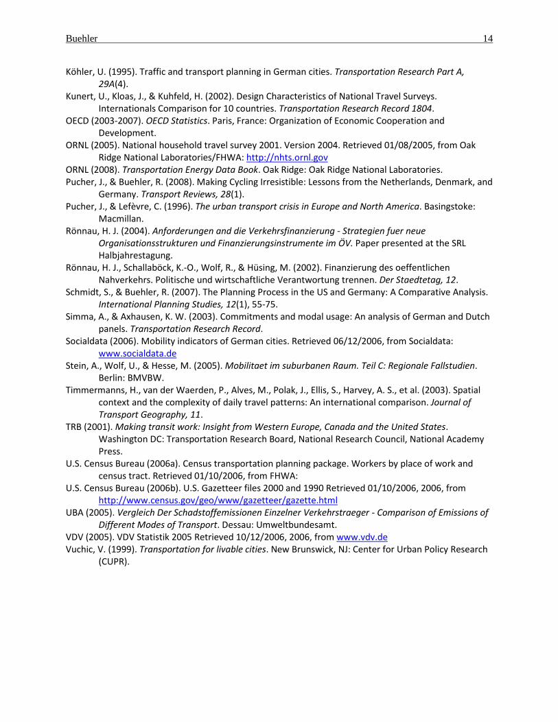
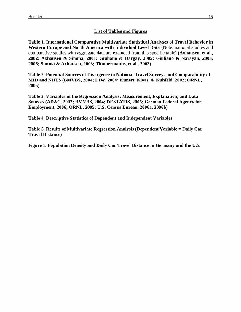
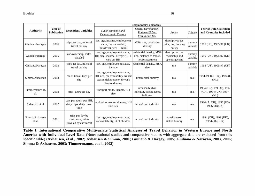
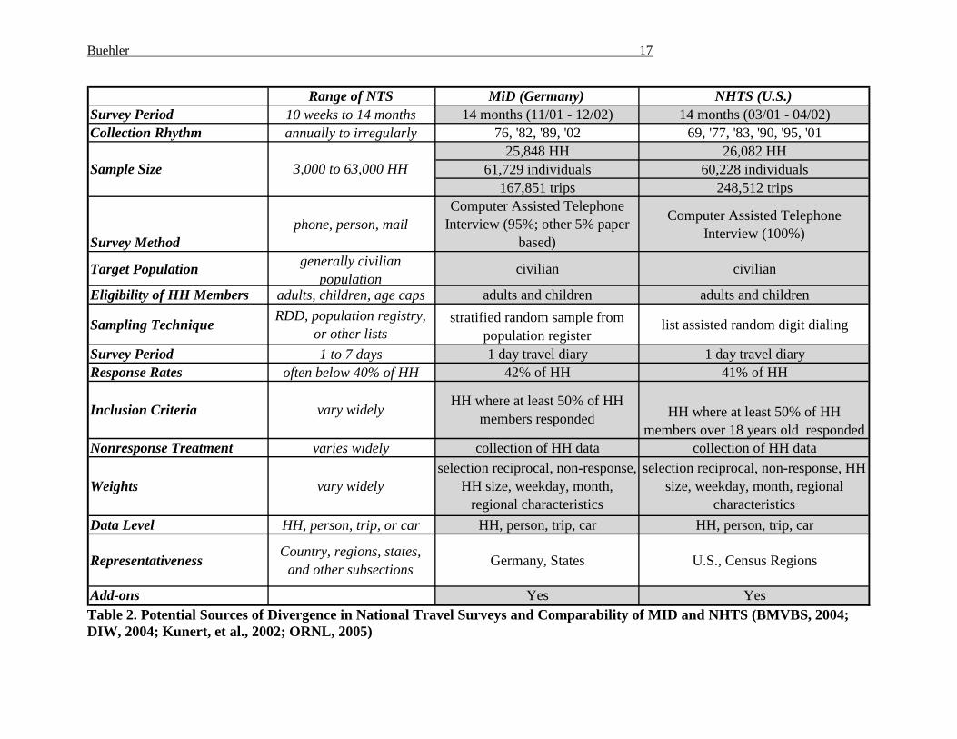
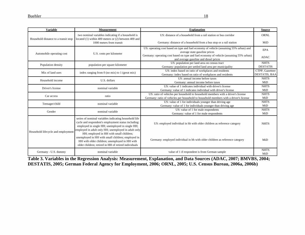
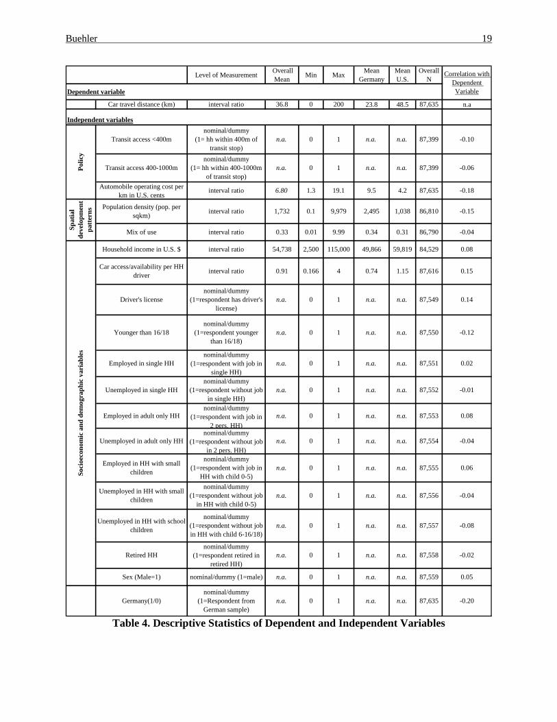
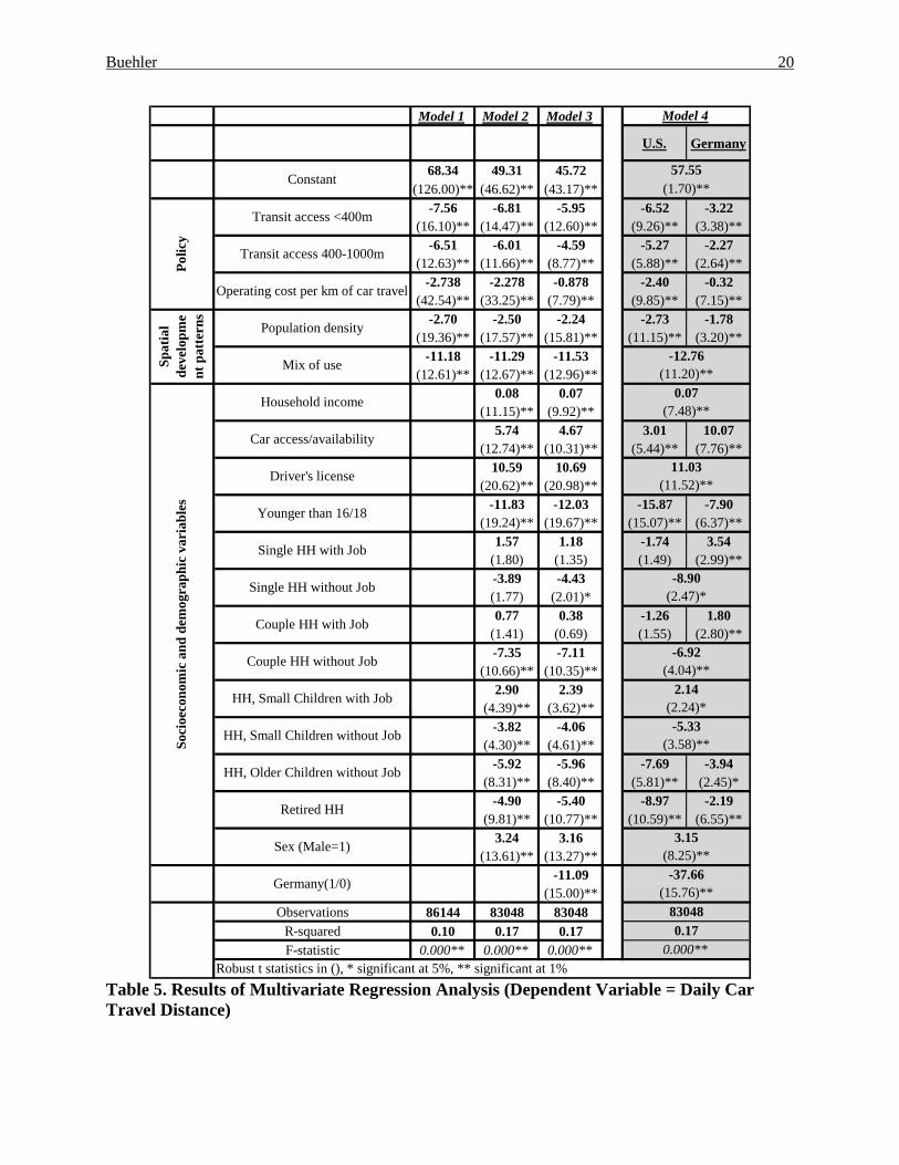
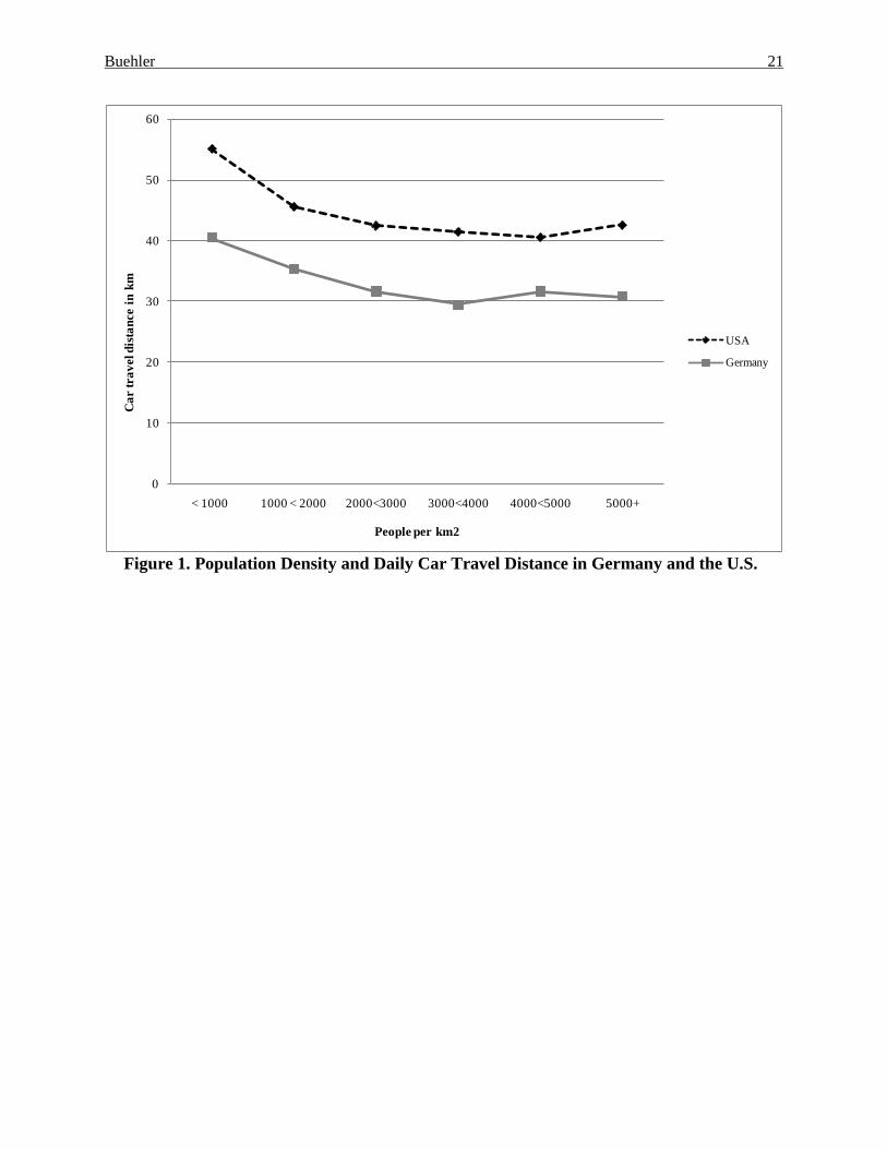
Buehler 21
0
10
20
30
40
50
60
lt 1000 1000 lt 2000 2000lt3000 3000lt4000 4000lt5000 5000+
Car
trav
el d
ista
nce
in k
m
People per km2
USA
Germany
Figure 1 Population Density and Daily Car Travel Distance in Germany and the US
Top Related