


Languages
Pages
Legal

1
Design of Marine Debris Removal System
Technical Report
Thomas Chrissley
Anthony Mason
Connor Maloy
Morgan Yang
Faculty Advisor: Dr. Lance Sherry
Sponsor: Mr. George Blaha, Raytheon
______________________________________________________
Department of System Engineering and Operation Research
George Mason University
4400 University Drive, Fairfax VA, 22030
May 1, 2017
2
Contents 1.0 Context Analysis ...................................................................................................................................... 5
1.1 Overview of Marine Debris ................................................................................................................. 5
1.2 Types and Source of Debris ................................................................................................................. 6
1.3 Movement of Debris ......................................................................................................................... 10
1.4 Impact of Debris ................................................................................................................................ 11
2.0 Stakeholder Analysis ............................................................................................................................. 12
2.1 Stakeholder Overview ....................................................................................................................... 12
2.2 Primary Stakeholders ........................................................................................................................ 12
2.3 Win-Win Analysis .............................................................................................................................. 13
3.0 Problem and Need Statement .............................................................................................................. 15
3.1 Problem Statement ........................................................................................................................... 15
3.2 Need Statement ................................................................................................................................ 15
4.0 Concept of Operations .......................................................................................................................... 16
5.0 Requirements ........................................................................................................................................ 17
5.1 Mission Requirements ...................................................................................................................... 17
5.2 Functional Requirements .................................................................................................................. 17
6.0 Technology Alternatives ....................................................................................................................... 18
6.1 Technology Alternatives Overview ................................................................................................... 18
6.2 Deploy Alternatives ........................................................................................................................... 18
6.3 Collection Alternatives ...................................................................................................................... 20
6.4 Retrieval Alternatives ........................................................................................................................ 22
6.5 Disposal Alternatives ......................................................................................................................... 23
7.0 Design Alternatives ............................................................................................................................... 25
7.1 Design Alternatives Overview ........................................................................................................... 25
7.2 Design Alternatives ........................................................................................................................... 25
7.2.1 Autonomous Vacuum ................................................................................................................ 26
7.2.2 Barge with Autonomous Surface Vehicle .................................................................................. 27
7.2.3 Barge with Unmanned Aerial Vehicle ........................................................................................ 28
7.2.4 Vessel with Nets ......................................................................................................................... 28
7.2.5 Artificial Floating Island .............................................................................................................. 29
7.2.6 Artificial Floating Island with Sail ............................................................................................... 30
7.2.7 Artificial Floating Island with Motor .......................................................................................... 30

3
8.0 Simulation ............................................................................................................................................. 31
8.1 Simulation Overview ......................................................................................................................... 31
8.2 Simulation Requirements ................................................................................................................. 31
8.3 Design of Experiment ........................................................................................................................ 31
8.4 Simulation Diagram ........................................................................................................................... 31
8.5 Simulation Parameters ...................................................................................................................... 32
8.6 Simulation Results ............................................................................................................................. 33
8.7 Simulation Verification ...................................................................................................................... 38
9.0 Utility Analysis ....................................................................................................................................... 39
9.1 Value Hierarchy ................................................................................................................................. 39
9.2 Attribute Weights ............................................................................................................................. 39
9.3 Design Alternatives Scores ................................................................................................................ 40
9.4 Sensitivity Analysis ............................................................................................................................ 40
10.0 Business Case ...................................................................................................................................... 44
9.1 Prospective Market ........................................................................................................................... 44
9.2 Business Model ................................................................................................................................. 44
9.3 Costs .................................................................................................................................................. 44
9.4 Annual Profit and Return on Investment .......................................................................................... 46
11.0 Project Plan ......................................................................................................................................... 49
11.1 Work Breakdown Structure ............................................................................................................ 49
11.2 Schedule .......................................................................................................................................... 50
11.3 Critical Path ..................................................................................................................................... 50
11.4 Budget ............................................................................................................................................. 51
11.5 Earned Value Management ............................................................................................................ 51
11.6 Project Risks and Risks Mitigation .................................................................................................. 52
References .............................................................................................................................................. 54
Appendix ..................................................................................................................................................... 56
Source Code ............................................................................................................................................ 56
A. Barge with Autonomous Surface Vehicle ....................................................................................... 56
B. Barge with Unmanned Aerial Vehicle ............................................................................................. 57
C. Autonomous Vacuum ..................................................................................................................... 58
D. Vessel with Nets............................................................................................................................. 59
E. Artificial Floating Island ................................................................................................................... 60

4
F. Artificial Floating Island with Sail .................................................................................................... 62
G. Artificial Floating Island with a Motor ............................................................................................ 64
H. Ocean Current Speed ...................................................................................................................... 66
I. Growth of amount of Debris ............................................................................................................ 67
J. Material Size Distribution ................................................................................................................ 67

5
1.0 Context Analysis
1.1 Overview of Marine Debris Debris is defined as the remains of anything broken down or destroyed [1]. Marine debris is defined as
any persistent solid material that is manufactured or processed and directly or indirectly, intentionally
or unintentionally, disposed of or abandoned into the marine environment [2]. There is not a part of the
world that is not touched by this problem [2]. The debris is a threat to our environment, navigation
safely, the economy, and human health [2]. Currently there is 8 million tons of debris or 8,000,000,000
kilograms (kg) in the North Pacific Ocean [2]. This number is estimated to increase 10% each year. The
graph below shows the increase of debris in kg, from what is currently in the ocean to what is expected
to be in 50 years (Source code in Appendix A, H). From that 8 million tons, about 30% of that debris is
floating of the surface of the ocean [2], while the rest of the debris sinks to the ocean floor.
Figure 1. Growth of the Marine Debris of 50 Years
This problem has become a “tragedy of the commons” problem. The “tragedy of the commons” is an
economic problem in which an individual tries to reap the greatest from a resource [3]. The resource in
the case in the marine environment, which everyone has the right to use. The individual in this case in
anyone who uses the marine environment for their benefit, this would include the fishing and marine
transportation industry as the biggest ones who benefit. These two industries are continuously using the
resource for their gain but they are not the ones are taking care of the problem, they are just adding to
the problem. But is not just them that is affecting the problem, it is everyone in the planet who is
contributing to the problem whether they know it or not. From this, it turns the problem of marine
6
debris into a cost problem. The reason that this a cost problem, is due the sheer amount of cost that is
needed to mitigate the harmful effects of the marine debris.
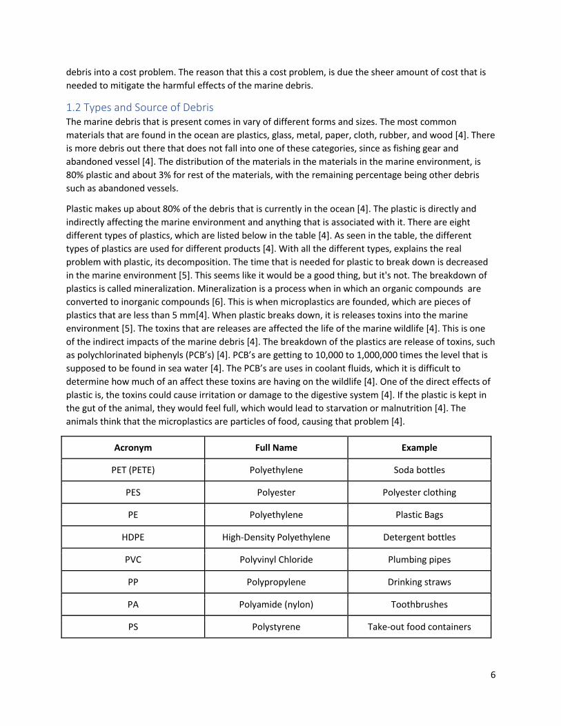
1.2 Types and Source of Debris The marine debris that is present comes in vary of different forms and sizes. The most common
materials that are found in the ocean are plastics, glass, metal, paper, cloth, rubber, and wood [4]. There
is more debris out there that does not fall into one of these categories, since as fishing gear and
abandoned vessel [4]. The distribution of the materials in the materials in the marine environment, is
80% plastic and about 3% for rest of the materials, with the remaining percentage being other debris
such as abandoned vessels.
Plastic makes up about 80% of the debris that is currently in the ocean [4]. The plastic is directly and
indirectly affecting the marine environment and anything that is associated with it. There are eight
different types of plastics, which are listed below in the table [4]. As seen in the table, the different
types of plastics are used for different products [4]. With all the different types, explains the real
problem with plastic, its decomposition. The time that is needed for plastic to break down is decreased
in the marine environment [5]. This seems like it would be a good thing, but it's not. The breakdown of
plastics is called mineralization. Mineralization is a process when in which an organic compounds are
converted to inorganic compounds [6]. This is when microplastics are founded, which are pieces of
plastics that are less than 5 mm[4]. When plastic breaks down, it is releases toxins into the marine
environment [5]. The toxins that are releases are affected the life of the marine wildlife [4]. This is one
of the indirect impacts of the marine debris [4]. The breakdown of the plastics are release of toxins, such
as polychlorinated biphenyls (PCB’s) [4]. PCB’s are getting to 10,000 to 1,000,000 times the level that is
supposed to be found in sea water [4]. The PCB’s are uses in coolant fluids, which it is difficult to
determine how much of an affect these toxins are having on the wildlife [4]. One of the direct effects of
plastic is, the toxins could cause irritation or damage to the digestive system [4]. If the plastic is kept in
the gut of the animal, they would feel full, which would lead to starvation or malnutrition [4]. The
animals think that the microplastics are particles of food, causing that problem [4].
Acronym Full Name Example
PET (PETE) Polyethylene Soda bottles
PES Polyester Polyester clothing
PE Polyethylene Plastic Bags
HDPE High-Density Polyethylene Detergent bottles
PVC Polyvinyl Chloride Plumbing pipes
PP Polypropylene Drinking straws
PA Polyamide (nylon) Toothbrushes
PS Polystyrene Take-out food containers
7
Another problem that is affecting wildlife is derelict fishing gear and abandoned vessels [4]. This type of
debris is causing a problem called ghost fishing. Ghost Fishing is an abandoned, lost, or dumped fishing
gear that continues to trap wildlife within it [7]. Even though the definition defines fishing gear as the
problem but abandoned vessel also have the chance to trap wildlife within them. The reason why ghost
fishing is a problem is that they are affecting already depleted commercial fish stocks [7]. The wildlife
that is caught will die and in turn attract scavenger which will get caught in the same gear, thus creating
a vicious circle [7]. The abandoned gear is among the greatest killers in our oceans, and not only because
of their numbers [7]. Hundreds of miles of nets and lines get lost every year and due to the materials,
that they are made of, they can keep fishing for multiple decades, or even centuries [7]. As stated
before, vessels also have the chance to cause the same problem. But one the biggest problems of an
abandoned vessel is the navigation hazard it creates in the waterways. So, of those vessels sink just
below the surface of the water making it very difficult to see it. Another vessel could hit it causing minor
to major damage or even potential sinking it.
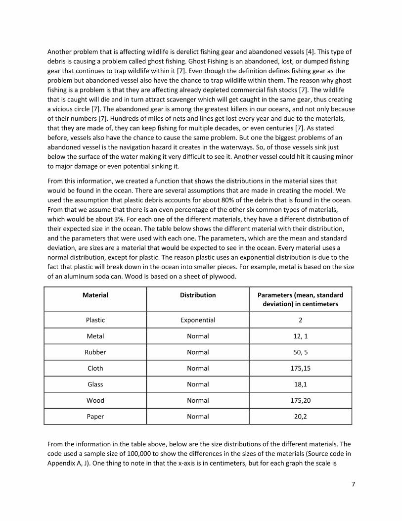
From this information, we created a function that shows the distributions in the material sizes that
would be found in the ocean. There are several assumptions that are made in creating the model. We
used the assumption that plastic debris accounts for about 80% of the debris that is found in the ocean.
From that we assume that there is an even percentage of the other six common types of materials,
which would be about 3%. For each one of the different materials, they have a different distribution of
their expected size in the ocean. The table below shows the different material with their distribution,
and the parameters that were used with each one. The parameters, which are the mean and standard
deviation, are sizes are a material that would be expected to see in the ocean. Every material uses a
normal distribution, except for plastic. The reason plastic uses an exponential distribution is due to the
fact that plastic will break down in the ocean into smaller pieces. For example, metal is based on the size
of an aluminum soda can. Wood is based on a sheet of plywood.
Material Distribution Parameters (mean, standard deviation) in centimeters
Plastic Exponential 2
Metal Normal 12, 1
Rubber Normal 50, 5
Cloth Normal 175,15
Glass Normal 18,1
Wood Normal 175,20
Paper Normal 20,2
From the information in the table above, below are the size distributions of the different materials. The
code used a sample size of 100,000 to show the differences in the sizes of the materials (Source code in
Appendix A, J). One thing to note in that the x-axis is in centimeters, but for each graph the scale is
8
different based on the mean and standard deviation for that material. As shown in the first graph, the
plastic sizes are very small which states that there is are thousands are pieces of microplastics. The
second image has six different subplots to show how each one of the different materials compare to one
another.
Figure 2. Distribution of Plastic Sizes

9
Figure 3. Distribution of Six Materials Found in the Ocean
The source of debris that is found in the marine environment is either land or sea-based [8]. Sea-based
sources account for 20% of the debris that is currently in the marine environment [8]. The materials that
turn into debris can be dumped, swept, or blown of vessel or stationary platforms that are at sea [8].
Three different categories sea-based sources are fishing vessels, stationary platforms, and cargo ships
and other vessels. Fishing vessels have fishing gear that may be lost from either commercial vessels or
recreational boats [8]. Stationary platforms, such as offshore oil or gas rigs, some of the things that are
lost are hard hats, gloves, and 55-gallon storage drums [8]. Cargo ships and other vessels have a chance
of losing freight, such as containers or even raw materials like wood logs [8]. Now, the land-based
sources include, storm water discharges, natural events, or littering, dumping, and poor waste
management [8]. Storm water discharge is water that flows along streets or the ground as a result of
rain or snow, this water has the able to carry debris with it [8]. Once the water reaches a storm drain, it
then is emptier into river, stream, canals, or even directly into ocean [8]. The debris that can be moved
by this water flow includes cigarette butts, medical items, food packaging, and containers [8]. Natural
events include hurricanes, tornadoes, tsunamis, floods and mudslides which have effects on human life
and property [8]. Floods or tidal surges are capable of carrying things that vary from cigarette butts to
roofs from houses is the affected area [8]. For example, in 2011, Japan was struck by a tsunami that was
cause by an earthquake [9]. The natural event destroyed and damaged countless building, including a
nuclear power plant. The National Oceanic and Atmospheric Administration (NOAA) saw that some of
the debris that was washed out to sea from the tsunami reached the United States and Canada over the
years since the event [9]. Littering, dumping, and poor waste management is the intentional or
unintentional disposal of domestic or industrial waste on land or in rivers can contribute to the marine

10
debris problem if a subsequent action carries the debris to the ocean[8]. An example of this problem is
the problem that the 2016 Olympic sailors faced in Rio De Janeiro, Brazil. A CNN article interviewed
several sailors that were competing in the competition, they talked about the debris that they had to
avoid [10]. One of the sailors stated that there were a lot of plastic bags that collected on the vessel,
while another stated that he need to dodge a chair [10]. The CNN article stated that the waters being
polluted by raw sewage [10]. This sewage is potentially dangerous for people who would swim in the
river [10].
1.3 Movement of Debris The movement of debris is affected by wind, ocean surface currents, and gyres. The different types of
materials will be affected differently from each one of the three source of movement. The speed and
distance that the debris will travel depend on the three different sources of movement. Below will
describe each one of the different types of movement.
Ocean winds is defined as the motion of the atmosphere relative to the surface of the ocean [11]. The
ocean winds are normally measured very close to the surface of the water, either by buoys, platforms,
and ships [11]. The most common reference height for near-surface ocean wind measurements is 10
meters above sea level [11]. The wind is measured using a mechanical anemometer, which uses the
wind to propel a very small turbine to determine the wind speed [11]. The winds speeds of the vary due
to several factors, i.e. seasonal changes. The winds affect the debris that is open to the air, an example
would be a log. The top of the log is visible and effected by the wind, while the bottom of the log is in
the water, which is affected by the ocean surface currents. For the table below shows a sample of the
data that is created from two different NOAA sites. The two different stations are Station 46006 and
Station 51101, both of which are on the closest stations to the Subtropical Convergence Zone (SCZ).
From the data that was collected over 5 years for each on the stations. The mean wind speed is 7.23 m/s
with a standard deviation of 3.46 m/s.
The ocean surface currents are created from the winds that blow on the surface of the ocean. The water
is moved in certain patterns because of the Earth’s spin and the Coriolis Effect [12]. The Coriolis Effect is
the result of Earth’s rotation on weather patterns and ocean currents [12]. This effect makes storms
swirl clockwise in the Southern Hemisphere and counterclockwise in the Northern Hemisphere [13]. The
winds are able to move the top 100 meters of the ocean, which are the surface ocean currents[12].
Surface currents flow in a regular pattern, but they are all not the same []. Some of the currents are
wide and shallow and other are deep and narrow [12]. The ocean surface currents are able to be
calculated from the wind speeds (calculation is shown in the Design Alternative Section). The ocean
surface currents are able to move everything that is the winds are not able too. The surface currents are
able to transport all types of debris, depending on the size of the debris with determine the speed that if
can travel.
A gyre is a large system of rotating ocean current that spiral around a central point, clockwise in the
Northern Hemisphere and counterclockwise in the Southern Hemisphere [4]. There are five gyres in the
world, which are the North and South Pacific Subtropical, the North and South Atlantic Subtropical, and
the Indian Ocean Subtropical gyre [4]. The most notable gyres in the North Pacific Subtropical gyre,
which is also known as the Great Pacific Garbage Patch (GPGP) [4]. The GPGP is created from four
different ocean current, which are the North Pacific, California, North Equatorial, and Kuroshio current
[4]. It is stated that if a piece of debris where to be dropped off the coast of California it would take six
11
years until it would reach the GPGP based on the four currents [4]. The exact size of the GPGP is difficult
to calculate due to the dynamics of the system [4]. From the currents that form the GPGP and the wind
and the ocean surface currents, there is another area that is known to concentrate debris [4]. This area
is called the Subtropical Convergence Zone (SCZ). The size of the SCZ is estimated to by 7 to 9 million
square miles, which includes the GPGP [4].
1.4 Impact of Debris There are some serious impacts from this problem which are habitat damage, wildlife entanglement and
ghost fishing, ingestion, economic loss, vessel damage, navigation hazards, and alien species transport
[4]. The first problem is habitat damage, which is the that debris can scour, break, smother, and
otherwise damage important habitats, like coral reefs [4]. Many of these habitats serve as the basis of
marine ecosystems and are critical to the survival of many other species [4]. The wildlife entanglement
and ghost fishing, as stated before, derelict nets, ropes, line or other fishing gear, can wrap around
marine life [4]. The entanglement can lead to injury, illness, suffocation, starvation, and even death [4].
Sea turtles, seabirds, and marine mammals have been known to ingest debris. The debris is mistaken for
food and ingested, the natural food may be attached to the debris, or the debris may have been
ingested accidentally with other food [4]. The ingestion of the debris may lead to loss of nutrition,
internal injury, intestinal blockage, starvation, and even death [4]. This are all the problems that marine
wildlife face with the debris.
The economic loss is seen across multiple industries. Two the biggest industries that are affected by the
marine debris are the fishing and marine transportation industry. The fishing industry is losing money to
the increase in maintenance cost and the reduced number of fishable wildlife. If is estimated that the
there is a loss of $6,000 of marine life per acre, from debris entanglement and ghost fishing [14]. The 21
Asia-Pacific Economic Cooperation (APEC) released that, from those numbers, it is estimated that the
fishing industry is losing about $364 million per year [15]. The marine transportation industry in dealing
the same thing of increase maintenance cost and damages to vessels. APEC estimated that the marine
transportation industry is losing about $279 million per year [15].
12
2.0 Stakeholder Analysis
2.1 Stakeholder Overview The marine debris issue is a “tragedy of the commons”, meaning that everyone contributes to the
problem yet no one is willing contribute to the cleanup. Given that the SCZ is located in international
waters, nobody wants to take responsibility for the debris, so organizations and individuals will be
reluctant to provide any necessary funding. There are five major stakeholders of the system, which are
non-profit organizations, fishing industry, military, marine transportation industry, and competing
companies. From these stakeholders, there the only tension would be the competing companies against
MDRS. Each one wants to problem to be solved to benefit them, is some way.
2.2 Primary Stakeholders Listed below are the five primary stakeholders of the MDRS system. The stakeholders are all affected by
marine debris, one way or another. Some of the stakeholders are affected by the problem more than
others, which would be the fishing and marine transportation industry.
Non-profit Organizations
The number of non-profit organizations that focus on marine conservation has increased over the years.
Currently there is about 35 different organizations, each one has a different specialization somewhere in
the marine conservation area. These organization are affected by the problem by the way that they try
to solve and help with the problem. There are several non-profit organizations that are trying to clean
up some of the debris that is found on it in the marine environment. Most the cleanup efforts take place
on the land, like cleaning up beaches before the debris makes it into the ocean.
Fishing Industry
The fishing industry is affected by the problem is a major way. As stated in the Context Analysis, the
marine wildlife is being affected by this problem is many different ways. The fishermen are dealing with
a loss of wildlife to fish for. This is due to the debris affecting the wildlife, through entanglement and
ghost fishing. The fishing industry is losing about $364 million dollars from either vessel damage or
reduced fishing populations [15]. Currently, it is estimated that about $6,000 worth of marine wildlife
per acre is lost to entanglement or ghost fishing [14]
Military
The military is affected by this problem is that if is causing interference with their activities. The vessels
that they military uses are affected by the amount of debris that is found out in the ocean. The debris
could be causing extra damage to the hulls of the vessels or blocking the intakes. This problem could be
costing millions of dollars in damages to the vessels that the United States rely on.
Marine Transportation
The marine transportation industry is affected by the debris in the same way that the military is. The
debris is causing damages to the vessels either through hull damage or blockage of intakes. This extra
damage is causing the industry about $280 million every year [14]. This increase of the damage costs in
decrease the profit that the industry could be potentially making.
Competing Companies

13
Currently, there is only one other competing company, which is the The Ocean Cleanup. However, even
though this is a competing company, we all want to clean up the ocean to help the marine wildlife and
the marine environment. The Ocean Cleanup would potentially be taking away from some of the
potential revenue that the system would generate.
Below is a table that summaries all the stakeholders with their risks, objectives, and conflicts that they
may encounter.
Primary Stakeholder Risk Objective Conflict
Marine Environment Entanglement, ingestion, habitat
destruction
Cleaner waters Harming wildlife when collecting debris
Fishing Industry Lower fish quality, reduced amount of fish
to catch and sell
Cleaner waters and healthier wildlife
Marine Transportation
Military Vessel damage and navigation hazards
Less blockage for vessels
Vessel interference
Marine Transportation Vessel damage and navigation hazards
Cleaner waters and shipping lanes
Insurance, fishing, harbors, resources
Competition Loss of profit Profit Expenses
Non-profit Organizations
Lack of funding Cleaner waters Expenses
2.3 Win-Win Analysis The following table shows the win-win analysis for each one of the stakeholders that was stated above.
As stated before, each one the stakeholders want the cleaner waters to benefit them is some way. The
benefit will be different for each one of the stakeholders. The fishing industry would benefit from
cleaner waters by, increase marine wildlife populations and healthier wildlife. The increase in wildlife
would in turn increase the profits for the industry. The military and marine transportation want to be
about to traverse the ocean in a more efficient and safer way. This would decrease the costs that both
are paying for damages to vessels.

14
Stakeholder Win Loss
Marine Environment Cleaner Waters -
Fishing Industry Healthier and more fish -
Military Clear waters and reduced costs -
Marine Transportation Cleaner waters and reduced costs
-
Non-profit Organizations Cleaner marine environment -
Competing companies Clean the debris faster Loss of profit

15
3.0 Problem and Need Statement
3.1 Problem Statement Marine debris is arming the marine wildlife through habitat damage, entanglement, ghost-fishing,
ingestion, and alien/invasive species transport. The marine transportation, military, and fishing industry
are also negatively impacted through economic loss, vessel damage and navigation hazards. This leads
to addition cost and reduced profits for the industries. Marine debris is associated with a cost of $1.2
billion to the 21 Asia-Pacific Economic Cooperation members [14].
3.2 Need Statement To migrate the harmful effects of marine debris on the marine wildlife, the debris must be removed
from the ocean before irreversible damage is done to the planet. There is a need for a removal system
that can traverse the ocean collecting the marine debris efficiently and safely.
16
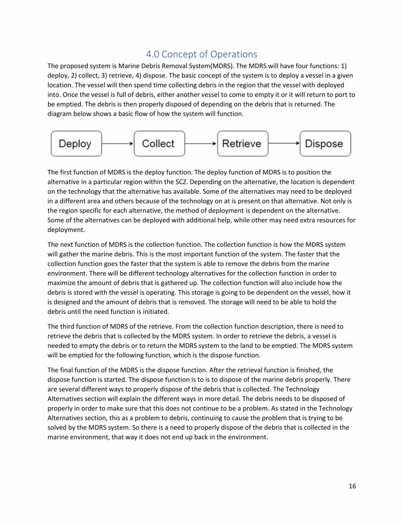
4.0 Concept of Operations The proposed system is Marine Debris Removal System(MDRS). The MDRS will have four functions: 1)
deploy, 2) collect, 3) retrieve, 4) dispose. The basic concept of the system is to deploy a vessel in a given
location. The vessel will then spend time collecting debris in the region that the vessel with deployed
into. Once the vessel is full of debris, either another vessel to come to empty it or it will return to port to
be emptied. The debris is then properly disposed of depending on the debris that is returned. The
diagram below shows a basic flow of how the system will function.
The first function of MDRS is the deploy function. The deploy function of MDRS is to position the
alternative in a particular region within the SCZ. Depending on the alternative, the location is dependent
on the technology that the alternative has available. Some of the alternatives may need to be deployed
in a different area and others because of the technology on at is present on that alternative. Not only is
the region specific for each alternative, the method of deployment is dependent on the alternative.
Some of the alternatives can be deployed with additional help, while other may need extra resources for
deployment.
The next function of MDRS is the collection function. The collection function is how the MDRS system
will gather the marine debris. This is the most important function of the system. The faster that the
collection function goes the faster that the system is able to remove the debris from the marine
environment. There will be different technology alternatives for the collection function in order to
maximize the amount of debris that is gathered up. The collection function will also include how the
debris is stored with the vessel is operating. This storage is going to be dependent on the vessel, how it
is designed and the amount of debris that is removed. The storage will need to be able to hold the
debris until the need function is initiated.
The third function of MDRS of the retrieve. From the collection function description, there is need to
retrieve the debris that is collected by the MDRS system. In order to retrieve the debris, a vessel is
needed to empty the debris or to return the MDRS system to the land to be emptied. The MDRS system
will be emptied for the following function, which is the dispose function.
The final function of the MDRS is the dispose function. After the retrieval function is finished, the
dispose function is started. The dispose function is to is to dispose of the marine debris properly. There
are several different ways to properly dispose of the debris that is collected. The Technology
Alternatives section will explain the different ways in more detail. The debris needs to be disposed of
properly in order to make sure that this does not continue to be a problem. As stated in the Technology
Alternatives section, this as a problem to debris, continuing to cause the problem that is trying to be
solved by the MDRS system. So there is a need to properly dispose of the debris that is collected in the
marine environment, that way it does not end up back in the environment.
17
5.0 Requirements The requirements for MDRS are derived a problem stated by our sponsor, which is to remove debris
from the marine environment. We developed this requirements from research about the problem,
through the context analysis. We have created High-Level Mission Requirements, which will explain
what MDRS. From that we break down into Functional Requirements, which explain how MDRS with
meet the Mission Requirements.
5.1 Mission Requirements 1. MDRS shall focus on the surface debris - where is within 3 meters deep of the surface
2. MDRS shall produce no extra debris
3. MDRS shall not harm any pre-existing ecosystem
4. MDRS shall remove 150,000,000 kg per year.
These requirements describe MDRS, based on the Concept of Operations. MDRS system will 1) Deploy,
2) Collection, 3) Retrieve, and 4) Dispose. The requirements states what each function should be able to
do.
5.2 Functional Requirements 1. MDRS shall deploy the system within the Subtropical Convergence Zone.
2. MDRS shall collect the debris from the marine environment into a collection area.
3. MDRS shall retrieve the debris and transport it back to land.
4. MDRS shall properly dispose of the debris that is removed.
18
6.0 Technology Alternatives
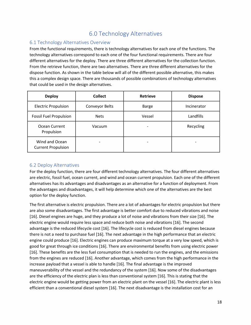
6.1 Technology Alternatives Overview From the functional requirements, there is technology alternatives for each one of the functions. The
technology alternatives correspond to each one of the four functional requirements. There are four
different alternatives for the deploy. There are three different alternatives for the collection function.
From the retrieve function, there are two alternatives. There are three different alternatives for the
dispose function. As shown in the table below will all of the different possible alternative, this makes
this a complex design space. There are thousands of possible combinations of technology alternatives
that could be used in the design alternatives.
Deploy Collect Retrieve Dispose
Electric Propulsion Conveyor Belts Barge Incinerator
Fossil Fuel Propulsion Nets Vessel Landfills
Ocean Current Propulsion
Vacuum - Recycling
Wind and Ocean Current Propulsion
- - -
6.2 Deploy Alternatives For the deploy function, there are four different technology alternatives. The four different alternatives
are electric, fossil fuel, ocean current, and wind and ocean current propulsion. Each one of the different
alternatives has its advantages and disadvantages as an alternative for a function of deployment. From
the advantages and disadvantages, it will help determine which one of the alternatives are the best
option for the deploy function.
The first alternative is electric propulsion. There are a lot of advantages for electric propulsion but there
are also some disadvantages. The first advantage is better comfort due to reduced vibrations and noise
[16]. Diesel engines are huge, and they produce a lot of noise and vibrations from their size [16]. The
electric engine would require less space and reduce both noise and vibrations [16]. The second
advantage is the reduced lifecycle cost [16]. The lifecycle cost is reduced from diesel engines because
there is not a need to purchase fuel [16]. The next advantage in the high performance that an electric
engine could produce [16]. Electric engines can produce maximum torque at a very low speed, which is
good for great through ice conditions [16]. There are environmental benefits from using electric power
[16]. These benefits are the less fuel consumption that is needed to run the engines, and the emissions
from the engines are reduced [16]. Another advantage, which comes from the high performance in the
increase payload that a vessel is able to handle [16]. The final advantage is the improved
maneuverability of the vessel and the redundancy of the system [16]. Now some of the disadvantages
are the efficiency of the electric plan is less than conventional system [16]. This is stating that the
electric engine would be getting power from an electric plant on the vessel [16]. The electric plant is less
efficient than a conventional diesel system [16]. The next disadvantage is the installation cost for an

19
electric plant and electric engines are higher [16]. The final disadvantage in the training that is required.
Currently, most crew members are training and understand how to operate a conventional system [16].
The electric system would require new or additional training [16].
Advantage Disadvantage
Better comfort due to reduced vibration and noise
Efficiency of electric plant is less than conventional system
Reduces lifecycle cost by less fuel consumption Installation cost are higher
High performance, maximum torque Different training
Environment benefits -
Increased payloads -
Improved maneuverability and redundancy -
The second alternative is fossil fuel propulsion. Fossil fuel propulsion has been one of the most sources
of propulsion on in the marine environment. The advantages of fossil fuels are its well developed and
cheap and reliable. The technology we use to harness the energy in fossil fuels are well developed [17].
This is way we are have been using fossil fuels for many years [17]. The second advantage is that fossil
fuel is cheap and reliable. They are great to an energy-base load, compared to other sources like wind
and solar [17]. However, there are several disadvantages to fossil fuels, which are contribute to global
warming, non-renewable, incentivized, and accidents happens [17]. The burning of fossil fuels is
releasing extra carbon which is a cause for global warming [17]. The next disadvantage is the fact that
fossil fuels are a non-renewable resource. This means that at some point we will run out, meaning that
the source of the fuel will run out [17]. And that it will take millions of years before that source will be
able again. The next disadvantage is that fossil fuels are incentivized. One of the reasons why fossil fuels
are cheap are due to the government incentives, coal, natural gas, and petroleum received $4.22 billion
in direct subsidies [17]. The final disadvantage is the accidents can happen. There is a potential for an
accident to happen, such as an oil spill or fuel leak [17]. Both of these events have the potential to cause
more problems than the one that is being solved. For example, Deepwater Horizon oil spill in the Gulf of
Mexico took years to clean up and the area is feeling the effect of the event.
Advantages Disadvantages
Well developed Affecting Global Warming
Cheap and Reliable Non-renewable
- Incentivized
- Accidents Happen

20
The third alternative for propulsion is ocean currents. There are couple of advantages to using ocean
currents, one of them is free source of propulsion. There is not energy of cost that would be needed in
order to use that ocean currents for propulsion. The next advantage in that it is very environmental
friendly. There is not power source or fuel that is required. As for disadvantages of the ocean currents,
there are not a reliable source. The speeds of the currents have a great deal of variability on them. The
ocean currents are based on the wind, which is not at a constant speed. The final disadvantage is the
speeds are slow. The average speed of the surface currents are about 0.015 m/s which is very slow. As
stated in the first disadvantage there is high variability in the speeds. The speed could be high but it will
not constantly but at a high rate.
Advantages Disadvantages
Free source of propulsion Not reliable
Environmental Friendly Slowest speeds
The fourth alternative is using ocean currents and the wind for propulsion. As stated in the ocean
currents above, the advantages and disadvantages are the same except adding the wind just adds some
more advantages and disadvantages. As stated, this alternative is free source of propulsion and
environmental friendly. Another advantage is that using ocean currents and winds is well developed.
Using ocean currents and wind to traverse the ocean has been used for more than 400 years. There a lot
of research and understanding of how they work together. The disadvantages are the same, not reliable
and slow speed. However, there is an add disadvantage which is an increased risk. The increased risk is
related to the potential for the sail to get damage, if there are high speeds.
Advantages Disadvantages
Free source of propulsion Not Reliable
Environmental friendly Slow speeds
Well developed Increased Risk
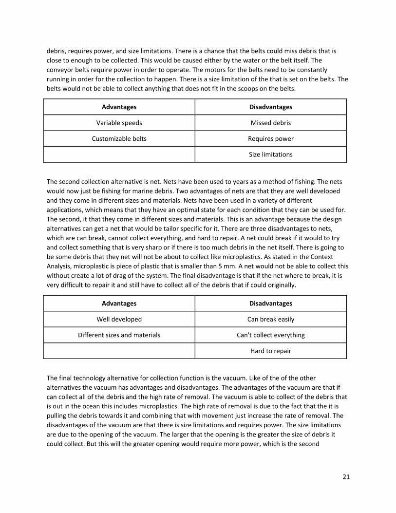
6.3 Collection Alternatives There are three different alternatives for the collection method of the system. They are conveyer belts,
nets, and vacuum. Each one of the different alternatives have advantages and disadvantages for how
they work and how they can collect the marine debris.
The first collection alternative is conveyer belts. Conveyor belts are used in a wide variety of different
applications. A couple of the advantages of conveyor belts are variable speeds and customizable belts.
The speeds of the belts can vary in speeds depending on the motor or what the code that runs the
motors for the belts. The second advantage is that the belts could be customized to the most efficient
way of removing debris from the marine environment. The belts could have scoops that would let the
scoop of the debris from the ocean. The conveyor belts have three disadvantages which are missed
21
debris, requires power, and size limitations. There is a chance that the belts could miss debris that is
close to enough to be collected. This would be caused either by the water or the belt itself. The
conveyor belts require power in order to operate. The motors for the belts need to be constantly
running in order for the collection to happen. There is a size limitation of the that is set on the belts. The
belts would not be able to collect anything that does not fit in the scoops on the belts.
Advantages Disadvantages
Variable speeds Missed debris
Customizable belts Requires power
Size limitations
The second collection alternative is net. Nets have been used to years as a method of fishing. The nets
would now just be fishing for marine debris. Two advantages of nets are that they are well developed
and they come in different sizes and materials. Nets have been used in a variety of different
applications, which means that they have an optimal state for each condition that they can be used for.
The second, it that they come in different sizes and materials. This is an advantage because the design
alternatives can get a net that would be tailor specific for it. There are three disadvantages to nets,
which are can break, cannot collect everything, and hard to repair. A net could break if it would to try
and collect something that is very sharp or if there is too much debris in the net itself. There is going to
be some debris that they net will not be about to collect like microplastics. As stated in the Context
Analysis, microplastic is piece of plastic that is smaller than 5 mm. A net would not be able to collect this
without create a lot of drag of the system. The final disadvantage is that if the net where to break, it is
very difficult to repair it and still have to collect all of the debris that if could originally.
Advantages Disadvantages
Well developed Can break easily
Different sizes and materials Can't collect everything
Hard to repair
The final technology alternative for collection function is the vacuum. Like of the of the other
alternatives the vacuum has advantages and disadvantages. The advantages of the vacuum are that if
can collect all of the debris and the high rate of removal. The vacuum is able to collect of the debris that
is out in the ocean this includes microplastics. The high rate of removal is due to the fact that the it is
pulling the debris towards it and combining that with movement just increase the rate of removal. The
disadvantages of the vacuum are that there is size limitations and requires power. The size limitations
are due to the opening of the vacuum. The larger that the opening is the greater the size of debris it
could collect. But this will the greater opening would require more power, which is the second

22
disadvantage. Running the vacuum over a large opening would require a lot of power it to run. There
needed to be a middle between the size of the opening and the power that is required.
Advantages Disadvantages
Collect all debris Size limitations
High rate of removal Requires Power
6.4 Retrieval Alternatives The first technology alternative for retrieval function is a barge. A barge is going to act as a “base of
operations” for the design alternatives that require it. The advantages of the barge are that there is no
labor cost and the operational cost is minimal. Since the barge will be unmanned, this means that there
is not labor cost associated with using it. There is a operational cost associated with a barge but it is
minimal, since the only cost would be maintenance or fuel that would be needed for that year. The
disadvantages of barge are that they are unmanned and not moveable. The disadvantage of having an
unmanned barge would be if something were to happen, then no one would be able to fix the problem.
The next is that a barge is not moveable, meaning that the barge requires another vessel to position the
barge in the correct location.
Advantages Disadvantages
No labor cost Unmanned
Operational Cost Not moveable
The vessel is the second technology alternative for the retrieval function. The vessel would has the
ability to be moveable and adaptable as the advantages. Moveable means that the vessel is able to
move on its own without the help of another vessel. Since the vessel requires a crew to operate it, it
gives them the ability to adapt any of the changing environment or conditions. The disadvantages of the
vessel are the labor cost that are associated with the crew would can be up to $50,000 per day
depending of the amount of crew that is needed to operate the ship. The second disadvantage is
operational cost of the vessel, which including the fuel, maintenance, and harboring cost. The most
expensive cost in the operational cost is the cost of fuel. A vessel could spend up to $10,000 per day in
fuel cost.
Advantages Disadvantages
Moveable Labor Costs
Adaptability Operational Cost

23
6.5 Disposal Alternatives There are three different alternatives for the dispose function of MDRS. They are incinerator, landfill,
and recycling. Each one of the different alternatives have advantages and disadvantages for how they
work and how they can collect the marine debris.
For the dispose technology alternatives, the first one is an incinerator. There are three advantages to using an incinerator and there are two disadvantages. The first advantage is that there is energy that is created from the process of using an incinerator [18] . The debris that is brought into the plant is burned, creating energy that can either heat or generate electricity for home [18]. The second advantage is better waste management [18]. An incinerator can burn up to 90% of the debris that is generated from a given area [18]. A landfill only facilitates the organic decomposition of the debris that is brought there [18]. The third advantage is the less dependence on landfills [18]. Being able to burn the debris would mean that there is less landfills that need to be created [18]. The disadvantages of incinerators is that they are not affordable and bad for the environment [18]. Incinerators are costly, in the creation of the plant and in the operation of the plant itself [18]. With burning the debris, they generate smoke, which can contain harmful toxins for the debris that is burned [18].
Advantages Disadvantages
Energy as Byproduct Not affordable
better waste management Bad of the environment
Less dependent on landfills -
The second alternative is the usage of landfills. There are three advantages of using a landfill, which are
minimize cost of export, gives energy, and safety. Landfills minimize cost of export because the debris
would not have to be transport to an isolated area [19] . So having the landfill close to the point of
where most debris is collected than it is reduced [19]. As the amount of debris is increases, the landfills
are able to collect methane that is created [19]. The methane that is created is able to be sold and
burned for energy production [19]. The next advantage is the safety that a landfill has. They are able to
safely deal with debris without the need of chemicals and containing the potential of created gases [19].
The disadvantage of landfills are the following, leachates, methane, and dust and pollution. The first
disadvantage of the landfills are leachates [19]. Leachates are when the toxins for the debris leak into
watershed, such as rain or snowfall [19]. The next disadvantage is the created of methane gas. If there
gas is not handled or contained, there is a chance that the gas would be harmful to the environment or
could ignite [19]. The final disadvantage is the dust and pollution that is created from it. The collection
of all the debris has the ability to create dust and pollution from the sheer amount of debris that is
brought to the location [19].

24
Advantages Disadvantages
Minimize cost of export Leachates
Gives Energy Methane
Safety Dust and pollution
The final technology alternative for dispose in recycling. There three advantages and two disadvantages
to using recycling. The first advantage is to minimize pollution, being able to recycle the debris means
that it would be used for other things, not ending up as pollution [20]. Next is that recycle protects the
environment, as stated in the first advantage, there is a decrease in pollution. This could help will with
the problem of marine debris as a whole [20]. The final advantage is the sustainable use of resources.
This means that instead of using something once, using it multiple times and then recycling it so it can
be used for something else [20]. The first disadvantage is that that recycling centers can unsafe [20].
There are unsafe with all the debris that is in the area and the use of chemicals on the debris [20]. The
second disadvantage is that recycling in not a widescale use in the world [20].
Advantages Disadvantages
minimize pollution Unsafe
Protects the environment Not widescale
Sustainable use of resources -
25
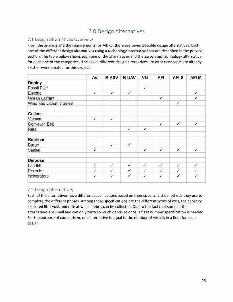
7.0 Design Alternatives
7.1 Design Alternatives Overview From the analysis and the requirements for MDRS, there are seven possible design alternatives. Each
one of the different design alternatives using a technology alternative that are described in the previos
section. The table below shows each one of the alternatives and the associated technology alternative
for each one of the categories. The seven different design alternatives are either concepts are already
exist or were created for this project.
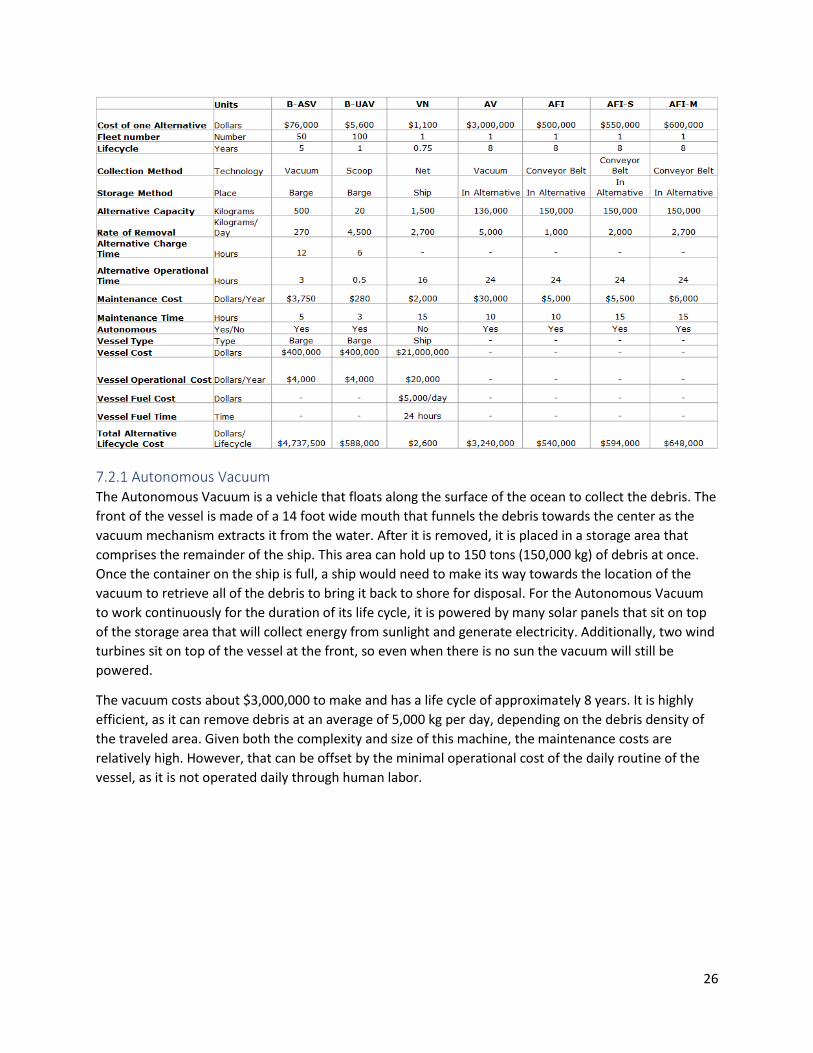
7.2 Design Alternatives Each of the alternatives have different specifications based on their sizes, and the methods they use to
complete the different phases. Among these specifications are the different types of cost, the capacity,
expected life cycle, and rate at which debris can be collected. Due to the fact that some of the
alternatives are small and can only carry so much debris at once, a fleet number specification is needed.
For the purpose of comparison, one alternative is equal to the number of vessels in a fleet for each
design.
26
7.2.1 Autonomous Vacuum The Autonomous Vacuum is a vehicle that floats along the surface of the ocean to collect the debris. The
front of the vessel is made of a 14 foot wide mouth that funnels the debris towards the center as the
vacuum mechanism extracts it from the water. After it is removed, it is placed in a storage area that
comprises the remainder of the ship. This area can hold up to 150 tons (150,000 kg) of debris at once.
Once the container on the ship is full, a ship would need to make its way towards the location of the
vacuum to retrieve all of the debris to bring it back to shore for disposal. For the Autonomous Vacuum
to work continuously for the duration of its life cycle, it is powered by many solar panels that sit on top
of the storage area that will collect energy from sunlight and generate electricity. Additionally, two wind
turbines sit on top of the vessel at the front, so even when there is no sun the vacuum will still be
powered.
The vacuum costs about $3,000,000 to make and has a life cycle of approximately 8 years. It is highly
efficient, as it can remove debris at an average of 5,000 kg per day, depending on the debris density of
the traveled area. Given both the complexity and size of this machine, the maintenance costs are
relatively high. However, that can be offset by the minimal operational cost of the daily routine of the
vessel, as it is not operated daily through human labor.

27
7.2.2 Barge with Autonomous Surface Vehicle The Barge with Autonomous Surface Vehicles is an alternative that consists of a fleet of relatively small
vehicles that collect debris, as well as a barge where the debris is stored when the vehicles are full. The
autonomous surface vehicles are four by ten meter floating bins that float over the debris to collect it.
Once the debris is extracted from the water, a compactor condenses the trash in the bin, so the vehicle
can collect until its capacity of 500 kg is met. Once the vehicle is full, it travels back to the barge it came
from to be emptied. While it is emptied, it is recharged from a solar powered charging station at the
barge before being dispatched to retrieve more debris. Given the smaller size of these vehicles, a fleet of
50 is necessary in order to clean the ocean at an effective rate. The barge associated with this
alternative is a floating storage area of which the vehicles are dispersed in all surrounding directions in
order to collect debris. A geofencing mechanism determines the area around the barge to be cleaned for
each vehicle. Similarly to the vacuum, the barge is emptied by a ship and crew that bring the debris back
to shore for proper disposal.
Each autonomous surface vehicle costs about $76,000 to make and has a life cycle of about 5 years. The
barges also cost about $400,000 to make. The vehicles collect debris at an average rate of 27o kg per
day, which means that they would return to the barge about once a day or once every two days,
depending on the amount of debris they are holding, as well as the charge they have left.

28
7.2.3 Barge with Unmanned Aerial Vehicle The Barge with Unmanned Aerial Vehicles is an alternative that acts similarly to the Barge with
Autonomous Surface Vehicles. The only differences with this option are that unmanned aerial vehicles
take the place of the surface vehicles. These are small drones that will venture off from the barge to a
given distance and drag a net along the ocean surface to collect debris. They are charged at the barge in
the same manner as the ASV’s. Each drone vehicle can hold a maximum of 20 kg, so there trips are quick
and frequent. Given this very low capacity, a fleet of 100 drones is necessary in order for this alternative
to be competitive with the other options. Each drone costs $5,600 to make and has a life cycle of about
one year. The details for the barge remain the same as the barge details in the ASV alternative.
7.2.4 Vessel with Nets The Vessel with Nets is the only alternative with already existing technology that could be deployed
immediately. While the others are concepts or in the prototype stage, the vessel with nets is simply a
large ship that drags nets along the side that collect debris floating on the surface. It would cost about
$1,100 to make nets of the appropriate size and strength and they would have a life cycle of about 9
months each. They can hold up to 1,500 kg, which is the rate of removal per day, so theoretically
speaking they will fill up to capacity with debris each day.
29
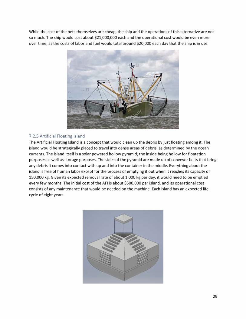
While the cost of the nets themselves are cheap, the ship and the operations of this alternative are not
so much. The ship would cost about $21,000,000 each and the operational cost would be even more
over time, as the costs of labor and fuel would total around $20,000 each day that the ship is in use.
7.2.5 Artificial Floating Island The Artificial Floating Island is a concept that would clean up the debris by just floating among it. The
island would be strategically placed to travel into dense areas of debris, as determined by the ocean
currents. The island itself is a solar powered hollow pyramid, the inside being hollow for floatation
purposes as well as storage purposes. The sides of the pyramid are made up of conveyor belts that bring
any debris it comes into contact with up and into the container in the middle. Everything about the
island is free of human labor except for the process of emptying it out when it reaches its capacity of
150,000 kg. Given its expected removal rate of about 1,000 kg per day, it would need to be emptied
every few months. The initial cost of the AFI is about $500,000 per island, and its operational cost
consists of any maintenance that would be needed on the machine. Each island has an expected life
cycle of eight years.
30
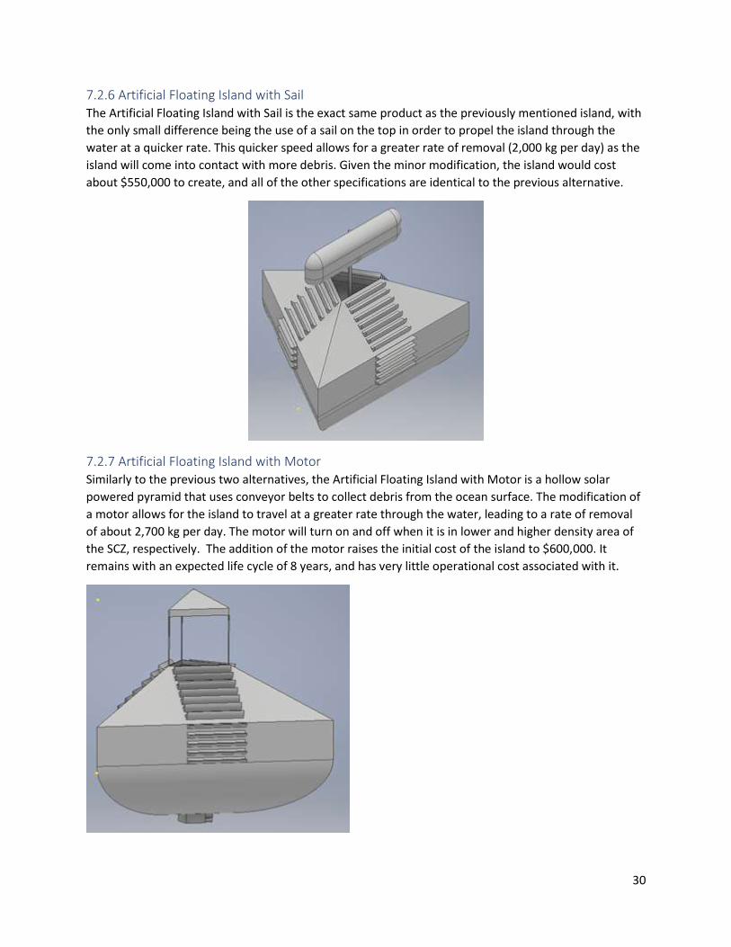
7.2.6 Artificial Floating Island with Sail The Artificial Floating Island with Sail is the exact same product as the previously mentioned island, with
the only small difference being the use of a sail on the top in order to propel the island through the
water at a quicker rate. This quicker speed allows for a greater rate of removal (2,000 kg per day) as the
island will come into contact with more debris. Given the minor modification, the island would cost
about $550,000 to create, and all of the other specifications are identical to the previous alternative.
7.2.7 Artificial Floating Island with Motor Similarly to the previous two alternatives, the Artificial Floating Island with Motor is a hollow solar
powered pyramid that uses conveyor belts to collect debris from the ocean surface. The modification of
a motor allows for the island to travel at a greater rate through the water, leading to a rate of removal
of about 2,700 kg per day. The motor will turn on and off when it is in lower and higher density area of
the SCZ, respectively. The addition of the motor raises the initial cost of the island to $600,000. It
remains with an expected life cycle of 8 years, and has very little operational cost associated with it.
31
8.0 Simulation
8.1 Simulation Overview The simulation is designed to test each one of the seven different design alternatives to give the best
utility value. The end goal is to see how each alternatives fair in terms of cost, efficiency, and time that is
needed to clean up the SCZ.
8.2 Simulation Requirements 1. The simulation shall model each design alternative as closely as possible.
2. The simulation shall generate a distribution of debris based on research data.
3. The simulation shall determine the utility of design alternatives by time and cost.
4. The simulation shall generate all possible data form random distributions based on collected
research.
8.3 Design of Experiment The table below shows the design of experiment for the simulation. The goal of the design of
experiment is to see how the output (rate of removal, cost, and time) and affected by the inputs
(alternative, fleet, speed, and collection method). The table shows a simple design of experiment, it
does not show all of the different levels that the inputs could be changed.
8.4 Simulation Diagram Below is a diagram showing how the MDRS simulation works. The inputs are the debris amount and
debris density. The uncontrollable variable is the drift rate and current speed. The parameters for the
simulation are speed of the vessel, debris collection method, operational time/ downtime, hourly cost,
and the non-recurring cost. The outputs of the simulation are the amount of debris that is collected, the
cost of operation, and the time that is needed to collect the debris.

32
8.5 Simulation Parameters The parameters of the simulation are the speed of the vessel, debris collection method, operating
time/downtime, hourly cost, and non-recurring cost that is associated with each of the different design
alternatives.
The speed of the vessel is dependent of the alternative. For example, the vessel with nets could go
faster than the speed that is input into the simulation, but the speed in limited by the nets. The nets are
creating a drag force that is acting against the vessel. Another limitation is the nets themselves, the
vessel has to travel at a low speed in order to the nets to collet everything and to reduce the risk of the
nets breaking for the debris. Each one of the different alternatives can travel at a different speed, so can
go at a faster speed, while others need to travel slower. The reasoning why each one has to travel at a
different speed is due to the different collection method.
The collection method is different for each of the alternatives. The collection method as stated in the
Technology Alternatives section and in the Design Alternatives section, each alternative has a different
collection method. The three different collection method works in different ways for each of the
alternatives. Some of the methods are better than ones but when paired with the rest of the technology
alternatives it makes for a good combination. The different collection methods require different things,
making the collection method one of the most important parameters.
The third parameter for the simulation is the operational time and downtime of each alternative.
Depending on the collection method and the speed of the vessel, which determine the rate of removal.
The rate of removal is going to be the operational time. When the capacity of the design alternatives is
full, it needed to be emptied. When the system needed to be emptied is going to be the downtime. The
reason why this is the downtime is because the system cannot collect any debris.
33
The hourly cost is the cost that is associated with operating the system per hour. Each one of the design
alternatives have different costs that are associated with it. The costs for each system is dependent on
the technology alternatives and how the system runs. For example, the vessel with nets has the lowest
cost for the collection method, however it has a huge cost associated with labor to run the vessel.
The non-recurring cost is also dependent on the design alternative. The non-recurring cost are the
lifecycle costs, which means that every time the system reaches the end of the of its lifecycle it has to be
replaced. Each of the design alternatives have a different lifecycle and cost associated with that.
8.6 Simulation Results The section will discuss the results of the simulation. Each one of the alternatives was tested with the
same inputs. The inputs are the amount of debris that is currently in the ocean and the number of
replications. The amount of debris that is used is 8,000,000,000 kg and the number of replications at
10,000. One thing to note with each of the different graphs is the scale that is used for next of the
design alternatives. The x-axis which is the time, it changes the scale for the different alternatives.
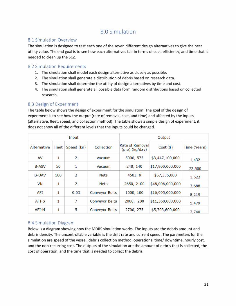
Below the output the simulation output for the autonomous vacuum. The graph shows the rate of
removal. The x-axis the is time in years for one autonomous vacuum to clean up the amount of debris
that is inputted. The y-axis is the rate of removal in kg per day. So, the graph is showing that the higher
the rate of removal it this less amount of time it will take. From this output, the mean rate of removal
for the autonomous vacuum is calculated. The autonomous vacuum’s mean rate of removal is 5,000 kg
per day.
Figure 5. Rate of Removal for Autonomous Vacuum
34
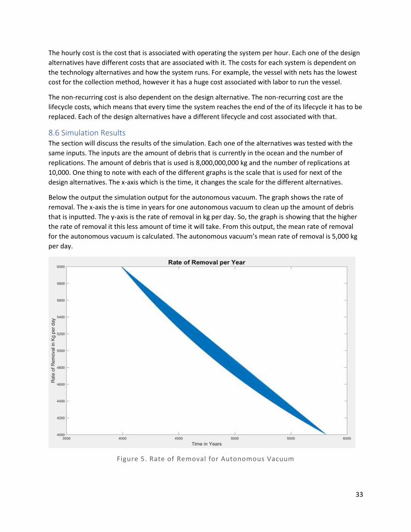
This graphs below are for the barge with autonomous surface vehicle. There are two graphs to show the
difference between with a fleet of 50 and without a fleet. The first graph shows the rate of removal for
just one ASV, however the second graph shows the rate of removal for a fleet of 50 ASVs. There second
graphs has a increased rate of removal from 15 to 500 kg per day. The mean rate of removal for the ASV
without a fleet is 9.86 kg/day with a standard deviation of 2.78, while with fleet of 50 ASVs the mean is
248.41 kg/day with a standard deviation of 139.39 kg/day.
Figure 6. Rate of Removal for One B-ASV

35
Figure 7. Rate of Removal for Fleet of B -ASV
The two graphs below show the rate of removal for the Barge with unmanned aerial vehicles. The first
graph shows the rate of removal of just one UVA, while the second graph shows a fleet of 100 UVAs. The
fleet number is chosen based on the cost of the UVAs and how the optimal way that the rate of removal
is increased. For the first graph, the maximum that a single UVA is able to handle in is 60 kg/day. The
mean for a single UVA is 44.88 kg/day with a standard deviation. However, with the fleet of 100 UVAs,
the maximum is 6,000 kg/day, with a mean of 4,503 kg/day and a standard deviation of 9.28 kg/day.

36
Figure 8. Rate of Removal for One B-UAV
Figure 9. Rate of Removal of Fleet of B -UAV
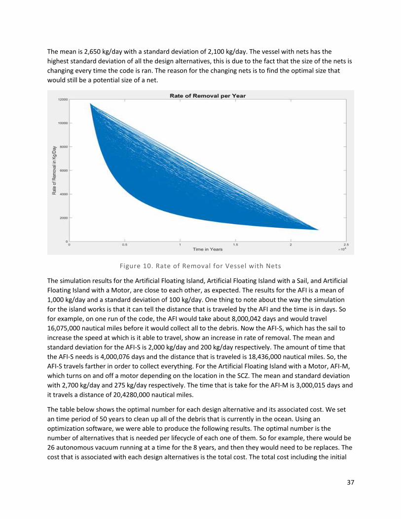
The graph below shows the rate of removal for the vessel with nets. The vessel with nets, has something
that is different from the other alternatives. The size of the nets is changed with next replication, but the
speed of the vessel is constant. This changed the mean and standard deviation of the rate of removal.
37
The mean is 2,650 kg/day with a standard deviation of 2,100 kg/day. The vessel with nets has the
highest standard deviation of all the design alternatives, this is due to the fact that the size of the nets is
changing every time the code is ran. The reason for the changing nets is to find the optimal size that
would still be a potential size of a net.
Figure 10. Rate of Removal for Vessel with Nets
The simulation results for the Artificial Floating Island, Artificial Floating Island with a Sail, and Artificial
Floating Island with a Motor, are close to each other, as expected. The results for the AFI is a mean of
1,000 kg/day and a standard deviation of 100 kg/day. One thing to note about the way the simulation
for the island works is that it can tell the distance that is traveled by the AFI and the time is in days. So
for example, on one run of the code, the AFI would take about 8,000,042 days and would travel
16,075,000 nautical miles before it would collect all to the debris. Now the AFI-S, which has the sail to
increase the speed at which is it able to travel, show an increase in rate of removal. The mean and
standard deviation for the AFI-S is 2,000 kg/day and 200 kg/day respectively. The amount of time that
the AFI-S needs is 4,000,076 days and the distance that is traveled is 18,436,000 nautical miles. So, the
AFI-S travels farther in order to collect everything. For the Artificial Floating Island with a Motor, AFI-M,
which turns on and off a motor depending on the location in the SCZ. The mean and standard deviation
with 2,700 kg/day and 275 kg/day respectively. The time that is take for the AFI-M is 3,000,015 days and
it travels a distance of 20,4280,000 nautical miles.
The table below shows the optimal number for each design alternative and its associated cost. We set
an time period of 50 years to clean up all of the debris that is currently in the ocean. Using an
optimization software, we were able to produce the following results. The optimal number is the
number of alternatives that is needed per lifecycle of each one of them. So for example, there would be
26 autonomous vacuum running at a time for the 8 years, and then they would need to be replaces. The
cost that is associated with each design alternatives is the total cost. The total cost including the initial
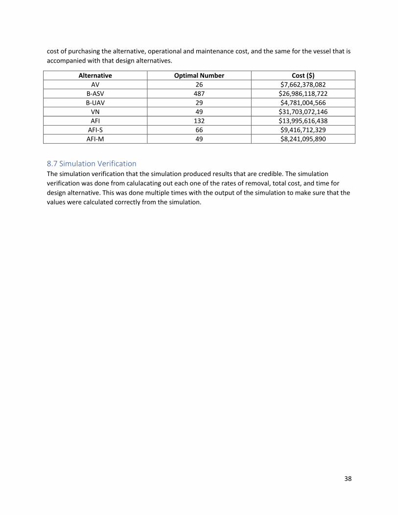
38
cost of purchasing the alternative, operational and maintenance cost, and the same for the vessel that is
accompanied with that design alternatives.
Alternative Optimal Number Cost ($)
AV 26 $7,662,378,082
B-ASV 487 $26,986,118,722
B-UAV 29 $4,781,004,566
VN 49 $31,703,072,146
AFI 132 $13,995,616,438
AFI-S 66 $9,416,712,329
AFI-M 49 $8,241,095,890
8.7 Simulation Verification The simulation verification that the simulation produced results that are credible. The simulation
verification was done from calulacating out each one of the rates of removal, total cost, and time for
design alternative. This was done multiple times with the output of the simulation to make sure that the
values were calculated correctly from the simulation.
39
9.0 Utility Analysis In order to properly identify the alternative that will be the most effective in cleaning up the ocean, a
utility analysis was conducted based on the categories listed below, and the respective specifications for
each alternative. Furthermore, a following utility vs. cost comparison helped show which alternatives
would be both effective, and financially feasible.
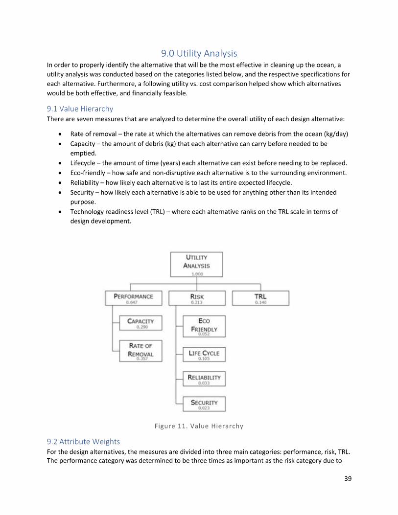
9.1 Value Hierarchy There are seven measures that are analyzed to determine the overall utility of each design alternative:
Rate of removal – the rate at which the alternatives can remove debris from the ocean (kg/day)
Capacity – the amount of debris (kg) that each alternative can carry before needed to be
emptied.
Lifecycle – the amount of time (years) each alternative can exist before needing to be replaced.
Eco-friendly – how safe and non-disruptive each alternative is to the surrounding environment.
Reliability – how likely each alternative is to last its entire expected lifecycle.
Security – how likely each alternative is able to be used for anything other than its intended
purpose.
Technology readiness level (TRL) – where each alternative ranks on the TRL scale in terms of
design development.
Figure 11. Value Hierarchy
9.2 Attribute Weights For the design alternatives, the measures are divided into three main categories: performance, risk, TRL. The performance category was determined to be three times as important as the risk category due to
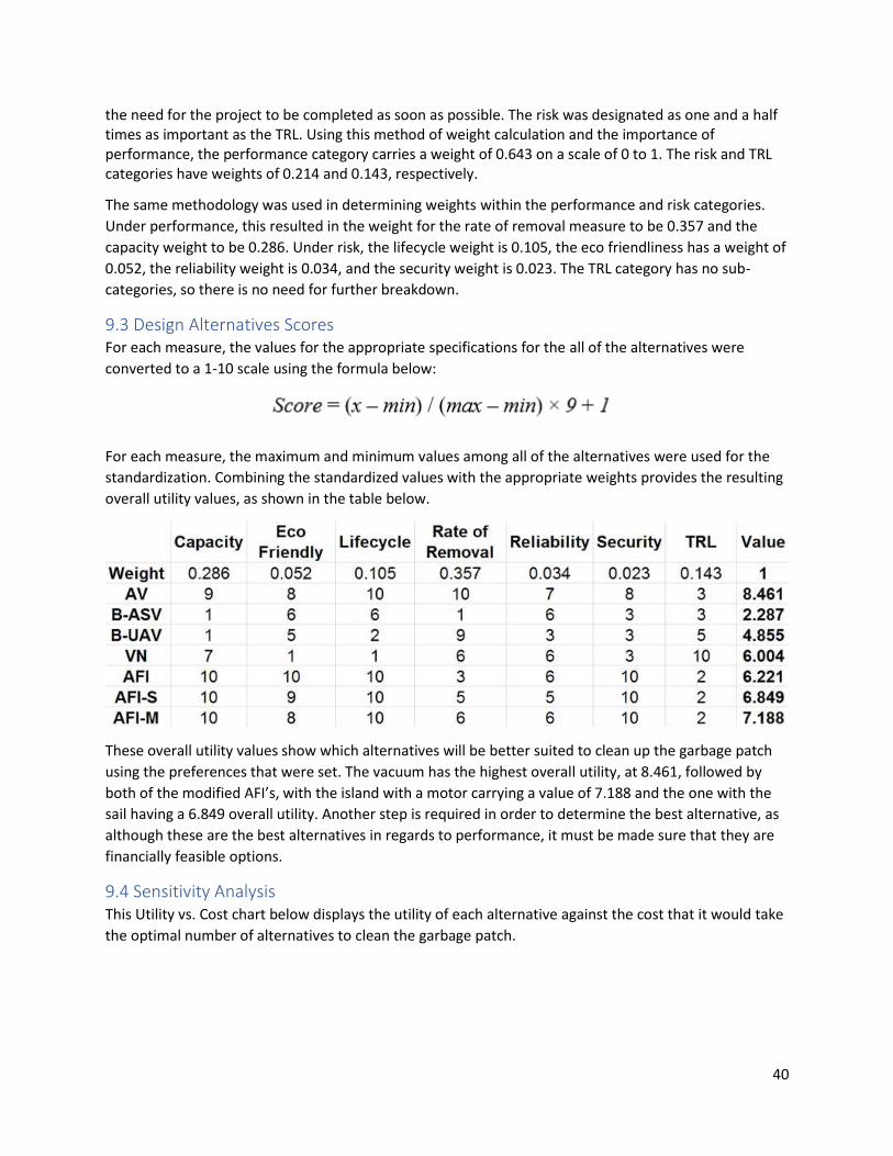
40
the need for the project to be completed as soon as possible. The risk was designated as one and a half times as important as the TRL. Using this method of weight calculation and the importance of performance, the performance category carries a weight of 0.643 on a scale of 0 to 1. The risk and TRL categories have weights of 0.214 and 0.143, respectively.
The same methodology was used in determining weights within the performance and risk categories.
Under performance, this resulted in the weight for the rate of removal measure to be 0.357 and the
capacity weight to be 0.286. Under risk, the lifecycle weight is 0.105, the eco friendliness has a weight of
0.052, the reliability weight is 0.034, and the security weight is 0.023. The TRL category has no sub-
categories, so there is no need for further breakdown.
9.3 Design Alternatives Scores For each measure, the values for the appropriate specifications for the all of the alternatives were
converted to a 1-10 scale using the formula below:
For each measure, the maximum and minimum values among all of the alternatives were used for the
standardization. Combining the standardized values with the appropriate weights provides the resulting
overall utility values, as shown in the table below.
These overall utility values show which alternatives will be better suited to clean up the garbage patch
using the preferences that were set. The vacuum has the highest overall utility, at 8.461, followed by
both of the modified AFI’s, with the island with a motor carrying a value of 7.188 and the one with the
sail having a 6.849 overall utility. Another step is required in order to determine the best alternative, as
although these are the best alternatives in regards to performance, it must be made sure that they are
financially feasible options.
9.4 Sensitivity Analysis This Utility vs. Cost chart below displays the utility of each alternative against the cost that it would take
the optimal number of alternatives to clean the garbage patch.
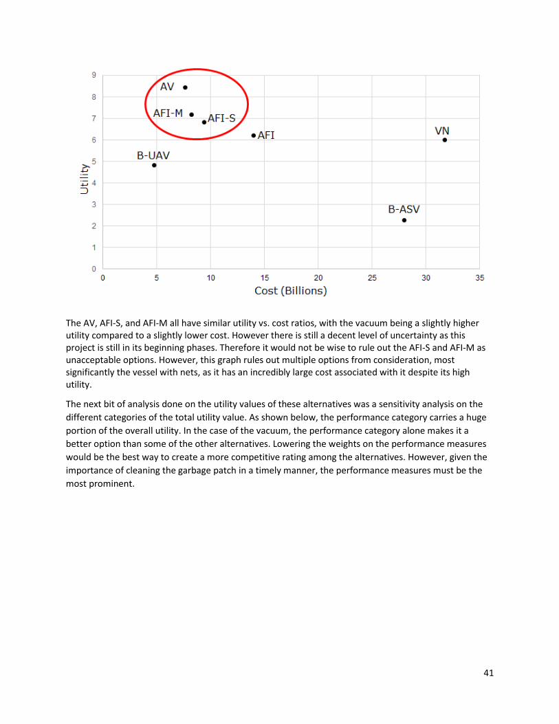
41
The AV, AFI-S, and AFI-M all have similar utility vs. cost ratios, with the vacuum being a slightly higher utility compared to a slightly lower cost. However there is still a decent level of uncertainty as this project is still in its beginning phases. Therefore it would not be wise to rule out the AFI-S and AFI-M as unacceptable options. However, this graph rules out multiple options from consideration, most significantly the vessel with nets, as it has an incredibly large cost associated with it despite its high utility.
The next bit of analysis done on the utility values of these alternatives was a sensitivity analysis on the
different categories of the total utility value. As shown below, the performance category carries a huge
portion of the overall utility. In the case of the vacuum, the performance category alone makes it a
better option than some of the other alternatives. Lowering the weights on the performance measures
would be the best way to create a more competitive rating among the alternatives. However, given the
importance of cleaning the garbage patch in a timely manner, the performance measures must be the
most prominent.

42
Figure 11. Utility Analysis Chart
Sensitivity graphs further breakdown the impact that the performance category has on the overall
utility. This graph shows that no matter what the weight is for the performance categories (0-100%), the
vacuum will always remain the top option in regards to overall utility. What this means for the other
alternatives is that they must improve on their performance specifications and capabilities in order to be
competitive with the autonomous vacuum.
Similarly to the performance sensitivity graph, the graph on the risk category shows the vacuum as a
clear favorite. The other alternatives must improve on their risk measures in order to become a
considered option for this project. However, if the weight on the risk category was raised to about 80%

43
of the overall utility, the island would become the winning option. Given the necessity for performance
in this situation, that is not a plausible scenario and therefore would not be wise to base analysis on
that.

44
10.0 Business Case MDRS is a hypothetical startup company with the goal of mitigating debris out of the ocean to save the
marine environment, through an in-house revenue stream of selling plastic recyclables and selling our
services to various industries to mitigate their costs associated with debris damages.
9.1 Prospective Market Currently, there is an estimated 2.4 million tons of debris floating at the surface in the SCZ alone. There
is only one other major competitor, The Ocean Cleanup (TOC), that is attempting to remove the debris
in the SCZ. They currently have ~100% of the market, because they have prototypes in the waters
already. TOC claims to, optimistically, have the ability to remove 45,000 tons per year [21]. The MDRS
systems far surpasses their ability to extract debris; One vacuum can remove 2,010 tons per year, so a
fleet of 26 will remove 7,260 more tons than TOC in a single year. If MDRS takes 3 years to become fully
operational, TOC will have collected, optimistically, 135,000 tons, which is 5.6% of the SCZ. It will thus
take around 19 years to surpass what TOC has removed and take over the majority market, when
measuring by amount removed from the marine environment. When measuring by potential revenue,
MDRS is the only one selling services and going past the revenue from the debris itself.
9.2 Business Model From the previous section, there is 2.4 million tons of debris floating on the surface in the SCZ. There are
multiple users of the ocean waters. The primary revenue seekers on the ocean are the fishing and
shipping industries. Both of these industries are dependent on safe waters to traverse, and fishing adds
the need for clean habitats for good quality product and haul size. The ocean debris directly affects both
of these needs in a negative way. The debris is a hazard to the ship itself and may cause damages to the
hull and/or the engine/propellers. The debris is damaging or even destroying habitats and harming fish
populations. Both of these negative impacts cost the industries millions of dollars per year in potential
revenue. The Asia-Pacific Economic Cooperation (APEC) completed a study reporting on the financial
burdens of the marine debris on various stakeholders in the 21 countries it encompasses. They reported
a loss of $364M/year to fishing industries and $279M/year to shipping industries [22]. MDRS provides a
service to remove the debris in the ocean. Thus, (1) mitigating the harmful effects of the debris, allowing
for more revenue potential, and (2) less cost from damages. MDRS will reach out to multiple countries
who industries are affected by the debris. Possibly discuss their desired regions to clean first, while
selling the services to clean those regions. Another revenue stream will come from salvaging or utilizing
the debris itself for profit
9.3 Costs This whole project is centered around more than just the way the debris can be remove, but more
centered on how to clean the debris out at a minimal cost. Cost is the greatest barrier to a project of this
magnitude. Because of this magnitude of costs, this become a Tragedy of the Commons. The ocean and
all the debris in it are not owned by any individual, group, or nation, thus no one wishes to take the
responsibility of ensuing the cost to remove the debris. The goal is to mitigate as much cost as possible
to remove the debris. Much like many other systems, operational costs are the most expensive portion
of the total costs. Thus, mitigating operational costs through the implementation of some autonomous
factors have been considered.

45
The costs involved with making MDRS operational are made up into two main costs; the alternatives
cost and the retrieval cost. The alternative cost is dependent on the specific alternative, each one has
different cost that are associated with each one. Below is chart that shows the breakdown for each
alternative. The breakdown includes the cost of one alternative itself not including the barge,
maintenance cost per year, charging station cost if needed, modification cost if needed, and fleet
number if alternative requires it. The maintenance cost of all the the alternatives is 5% of the initial cost
of B-ASV and B-UAV, and a 1% of the initial cost the the remaining alternatives. The cost of nets is $0.30
per meter, the actual size of the nets is created in the simulation for the VN.
Barge with
ASV
Barge with
UAV
Autonomous
Vacuum
(AV)
Artificial
Floating
Island (AFI) AFI with Sail
AFI with
Motor
Vessel
with
Nets
Cost of One $75,000 $4,000 $3,000,000 $500,000 $550,000 $600,000 $0.30
Maintenance $3,750 $280 $30,000 $5,000 $5,500 $6,000 -
Charging
Station $2,000 $2,000 - - - - -
Modification
s $1,000 $1,600 - - - - -
Fleet
Number 50 100 - - - - -
Now there is a more cost that is associated with each alternative, being the “base of operations” and the
retrieval cost. B-ASV, B-UAV, and VN are the three alternatives that are dependent on each vessel. B-
ASV and B-UAV both rely on the use of a barge, with is specific operational cost. The VN requires a
vessel for constant use. Below shows a table that has the cost of vessel, fuel cost per day, modification
cost that may be need, and the operational cost for each vessel per year. The operation cost of the
vessel includes the crew, maintenance, and harboring cost that are associated with the vessel.
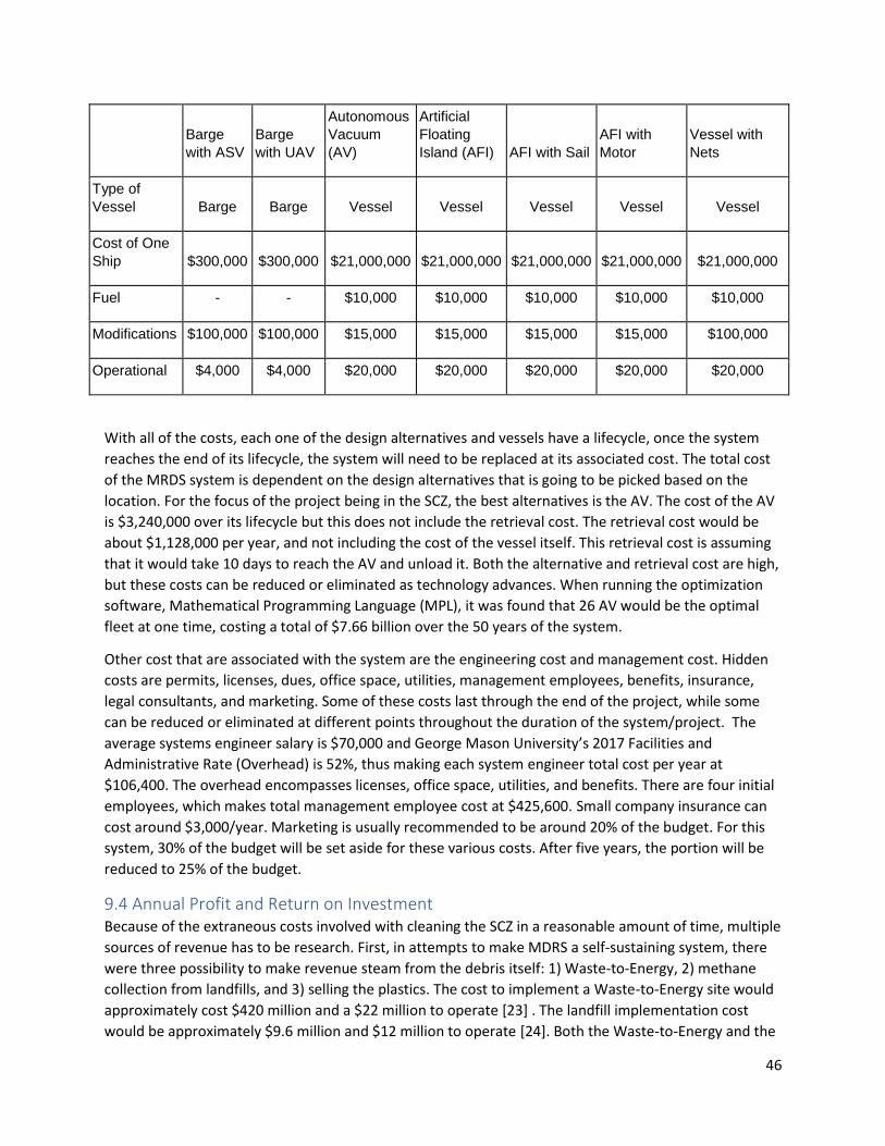
46
Barge
with ASV
Barge
with UAV
Autonomous
Vacuum
(AV)
Artificial
Floating
Island (AFI) AFI with Sail
AFI with
Motor
Vessel with
Nets
Type of
Vessel Barge Barge Vessel Vessel Vessel Vessel Vessel
Cost of One
Ship $300,000 $300,000 $21,000,000 $21,000,000 $21,000,000 $21,000,000 $21,000,000
Fuel - - $10,000 $10,000 $10,000 $10,000 $10,000
Modifications $100,000 $100,000 $15,000 $15,000 $15,000 $15,000 $100,000
Operational $4,000 $4,000 $20,000 $20,000 $20,000 $20,000 $20,000
With all of the costs, each one of the design alternatives and vessels have a lifecycle, once the system
reaches the end of its lifecycle, the system will need to be replaced at its associated cost. The total cost
of the MRDS system is dependent on the design alternatives that is going to be picked based on the
location. For the focus of the project being in the SCZ, the best alternatives is the AV. The cost of the AV
is $3,240,000 over its lifecycle but this does not include the retrieval cost. The retrieval cost would be
about $1,128,000 per year, and not including the cost of the vessel itself. This retrieval cost is assuming
that it would take 10 days to reach the AV and unload it. Both the alternative and retrieval cost are high,
but these costs can be reduced or eliminated as technology advances. When running the optimization
software, Mathematical Programming Language (MPL), it was found that 26 AV would be the optimal
fleet at one time, costing a total of $7.66 billion over the 50 years of the system.
Other cost that are associated with the system are the engineering cost and management cost. Hidden
costs are permits, licenses, dues, office space, utilities, management employees, benefits, insurance,
legal consultants, and marketing. Some of these costs last through the end of the project, while some
can be reduced or eliminated at different points throughout the duration of the system/project. The
average systems engineer salary is $70,000 and George Mason University’s 2017 Facilities and
Administrative Rate (Overhead) is 52%, thus making each system engineer total cost per year at
$106,400. The overhead encompasses licenses, office space, utilities, and benefits. There are four initial
employees, which makes total management employee cost at $425,600. Small company insurance can
cost around $3,000/year. Marketing is usually recommended to be around 20% of the budget. For this
system, 30% of the budget will be set aside for these various costs. After five years, the portion will be
reduced to 25% of the budget.
9.4 Annual Profit and Return on Investment Because of the extraneous costs involved with cleaning the SCZ in a reasonable amount of time, multiple
sources of revenue has to be research. First, in attempts to make MDRS a self-sustaining system, there
were three possibility to make revenue steam from the debris itself: 1) Waste-to-Energy, 2) methane
collection from landfills, and 3) selling the plastics. The cost to implement a Waste-to-Energy site would
approximately cost $420 million and a $22 million to operate [23] . The landfill implementation cost
would be approximately $9.6 million and $12 million to operate [24]. Both the Waste-to-Energy and the
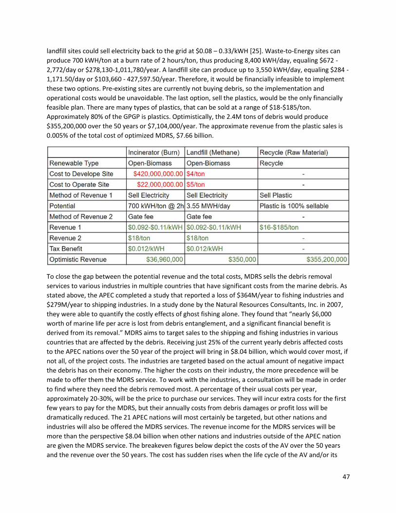
47
landfill sites could sell electricity back to the grid at $0.08 – 0.33/kWH [25]. Waste-to-Energy sites can
produce 700 kWH/ton at a burn rate of 2 hours/ton, thus producing 8,400 kWH/day, equaling $672 -
2,772/day or $278,130-1,011,780/year. A landfill site can produce up to 3,550 kWH/day, equaling $284 -
1,171.50/day or $103,660 - 427,597.50/year. Therefore, it would be financially infeasible to implement
these two options. Pre-existing sites are currently not buying debris, so the implementation and
operational costs would be unavoidable. The last option, sell the plastics, would be the only financially
feasible plan. There are many types of plastics, that can be sold at a range of $18-$185/ton.
Approximately 80% of the GPGP is plastics. Optimistically, the 2.4M tons of debris would produce
$355,200,000 over the 50 years or $7,104,000/year. The approximate revenue from the plastic sales is
0.005% of the total cost of optimized MDRS, $7.66 billion.
To close the gap between the potential revenue and the total costs, MDRS sells the debris removal
services to various industries in multiple countries that have significant costs from the marine debris. As
stated above, the APEC completed a study that reported a loss of $364M/year to fishing industries and
$279M/year to shipping industries. In a study done by the Natural Resources Consultants, Inc. in 2007,
they were able to quantify the costly effects of ghost fishing alone. They found that “nearly $6,000
worth of marine life per acre is lost from debris entanglement, and a significant financial benefit is
derived from its removal.” MDRS aims to target sales to the shipping and fishing industries in various
countries that are affected by the debris. Receiving just 25% of the current yearly debris affected costs
to the APEC nations over the 50 year of the project will bring in $8.04 billion, which would cover most, if
not all, of the project costs. The industries are targeted based on the actual amount of negative impact
the debris has on their economy. The higher the costs on their industry, the more precedence will be
made to offer them the MDRS service. To work with the industries, a consultation will be made in order
to find where they need the debris removed most. A percentage of their usual costs per year,
approximately 20-30%, will be the price to purchase our services. They will incur extra costs for the first
few years to pay for the MDRS, but their annually costs from debris damages or profit loss will be
dramatically reduced. The 21 APEC nations will most certainly be targeted, but other nations and
industries will also be offered the MDRS services. The revenue income for the MDRS services will be
more than the perspective $8.04 billion when other nations and industries outside of the APEC nation
are given the MDRS service. The breakeven figures below depict the costs of the AV over the 50 years
and the revenue over the 50 years. The cost has sudden rises when the life cycle of the AV and/or its

48
retrieval ship are ended and are replaced. The revenue is constant combining the revenue from the
plastics and the MDRS service.
Figure 13. Break-Even Graph over 50 Years
Figure 14. Break-Even Graph Close Up

49
11.0 Project Plan
11.1 Work Breakdown Structure The following hierarchy shows the different levels of the project as they are broken down. The
categories are based on deliverables and important tasks needed to complete the project. Below is the
Work Breakdown Structure.
Figure 15. Work Breakdown Structure
Management is the first task, which is the most important. There is meetings and sponsor interactions
that breakdown management. The meetings are meetings that the team has to discuss the project and
the work that needs to be done. The sponsor interactions is email and talking to the sponsor about the
direction of the project.
Next is research, which is broken down into background and design research. The background research
is important because we needed to get a better understanding of the problem and all of the factors that
affect the problem. The design research is all the research for each one of the different design
alternatives.
The next work function is the CONOPS, which is understand the what we need to do to solve the
problem.
That is followed by requirements. The requirements are broken down into mission and functional. The
mission requirements come from the CONOPS, stating what the system shall do. The functional
requirements come from the different functions within the CONOPS.
The fifth things is the design alternatives that are chosen based on the requirements. That is broken
down farther with components, which is related to the technology alternatives, each of the different
alternatives for the different functions.

50
Next is the analysis, which is broken down to cost, context, sensitivity, stakeholder, and tradeoff. Each
one these analyses, was completed to help understand the problem and how to the solve it given the
different design alternatives that were chosen based on the technology alternatives.
The seventh function in the work breakdown structure is the design. The design is the design of the
simulation and how it should work and what is included.
The next one is the simulation, this was actually coding out the simulation. The breakdown of this is the
modeling. Modeling is used for the AFI’s, since there that was a concept that was developed for the
project.
The final was is the testing of the simulation. We need to verify the simulation and validate it. The
verification is making sure that the simulation was created the correct values.
11.2 Schedule The schedule of the project is derived from the WBS and due dates. The schedule used a cyclical
approach by dividing the project into different phases based on the project briefings. Each of the project
briefing needed certain tasks to be completed before the briefing. After the briefing, we would receive
feedback that then would be part of the next phase of work.
11.3 Critical Path Below shows the schedule of the tasks that needed to be completed for the project. The red bars and
lines indicate the critical path. The tasks at are on the critical path are important to be finished on time,
if there are not finished on time then they would set up the schedule.
Figure 16. Critical Path
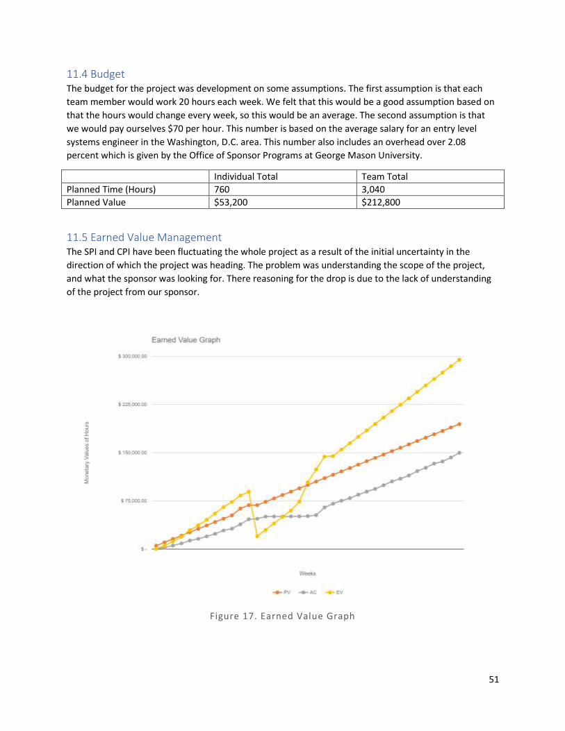
51
11.4 Budget The budget for the project was development on some assumptions. The first assumption is that each
team member would work 20 hours each week. We felt that this would be a good assumption based on
that the hours would change every week, so this would be an average. The second assumption is that
we would pay ourselves $70 per hour. This number is based on the average salary for an entry level
systems engineer in the Washington, D.C. area. This number also includes an overhead over 2.08
percent which is given by the Office of Sponsor Programs at George Mason University.
Individual Total Team Total
Planned Time (Hours) 760 3,040
Planned Value $53,200 $212,800
11.5 Earned Value Management The SPI and CPI have been fluctuating the whole project as a result of the initial uncertainty in the
direction of which the project was heading. The problem was understanding the scope of the project,
and what the sponsor was looking for. There reasoning for the drop is due to the lack of understanding
of the project from our sponsor.
Figure 17. Earned Value Graph
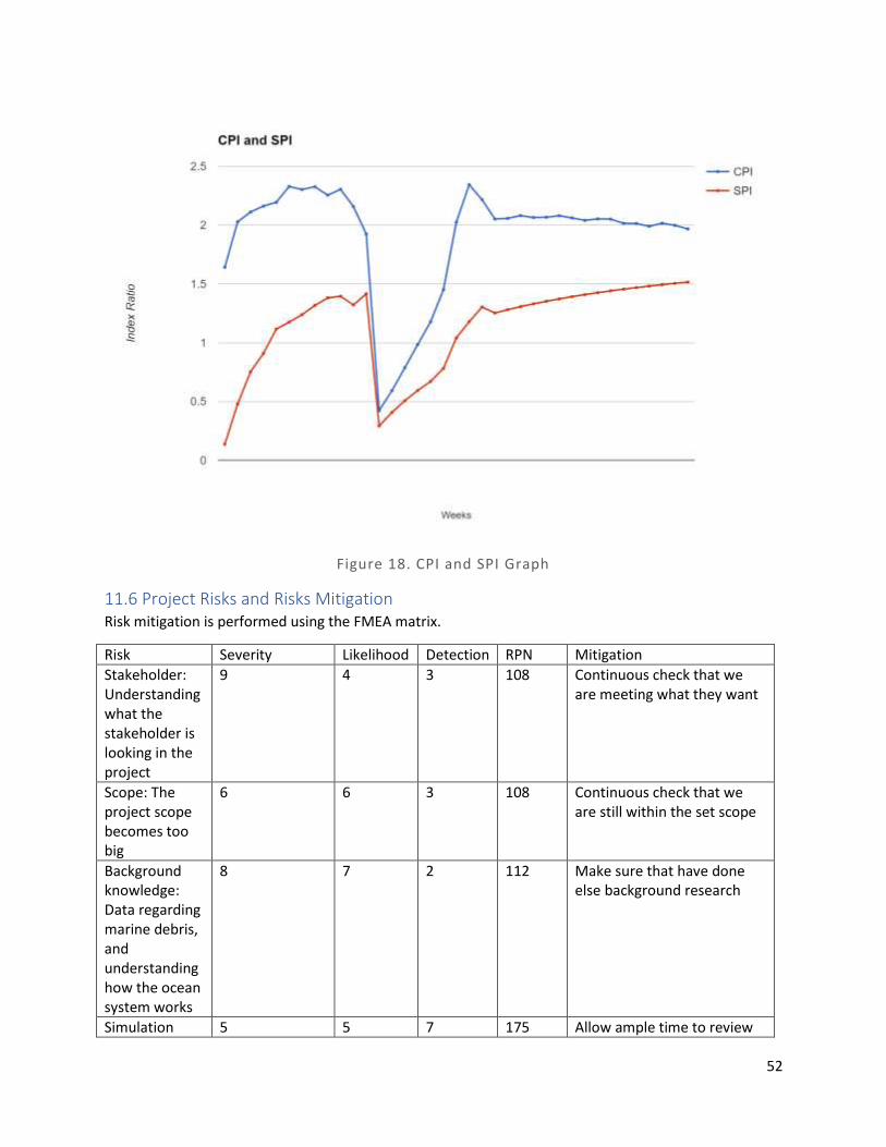
52
Figure 18. CPI and SPI Graph
11.6 Project Risks and Risks Mitigation Risk mitigation is performed using the FMEA matrix.
Risk Severity Likelihood Detection RPN Mitigation
Stakeholder: Understanding what the stakeholder is looking in the project
9 4 3 108 Continuous check that we are meeting what they want
Scope: The project scope becomes too big
6 6 3 108 Continuous check that we are still within the set scope
Background knowledge: Data regarding marine debris, and understanding how the ocean system works
8 7 2 112 Make sure that have done else background research
Simulation 5 5 7 175 Allow ample time to review

53
Issues: Outputting wrong values.
and verify that it correct
Resource Allocation: Teams ability to work and get the work done on the project.
8 3 2 48 Optimizing planning, budget and time
Severity: 1 (less severe) – 10 (very severe)
Likelihood: 1 (less likely) – 10 (most likely)
Detection: 1 (able to detection before problem) – 10 ( unable to detect before it happens)
54
References [1] - “debris,” Dictionary.com. [Online]. Available: http://www.dictionary.com/browse/debris?s=t.
[Accessed: 30-Apr-2017].
[2] - “| OR&R's Marine Debris Program,” | OR&R's Marine Debris Program. [Online]. Available:
https://marinedebris.noaa.gov/discover-issue/. [Accessed: 30-Apr-2017].
[3] I. Staff, “Tragedy Of The Commons,” Investopedia, 23-Nov-2015. [Online]. Available:
http://www.investopedia.com/terms/t/tragedy-of-the-commons.asp. [Accessed: 30-Apr-2017].
[4] - “OR&R's Marine Debris Program |,” OR&R's Marine Debris Program |. [Online]. Available:
https://marinedebris.noaa.gov/. [Accessed: 30-Apr-2017].
[5] “Plastics in oceans decompose, release hazardous chemicals, surprising new study says,” American
Chemical Society. [Online]. Available:
https://www.acs.org/content/acs/en/pressroom/newsreleases/2009/august/plastics-in-oceans-
decompose-release-hazardous-chemicals-surprising-new-study-says.html. [Accessed: 30-Apr-2017].
[6] Eni Generalic, Faculty of Chemistry and Technology, Split, Croatia, “CHEMISTRY
GLOSSARY,” Mineralization @ Chemistry Dictionary & Glossary. [Online]. Available:
http://glossary.periodni.com/glossary.php?en=mineralization. [Accessed: 30-Apr-2017].
[7] “Ghost Fishing,” Ghost Fishing. [Online]. Available: http://www.ghostfishing.org/. [Accessed: 30-Apr-
2017].
[8] “| OR&R's Marine Debris Program,” | OR&R's Marine Debris Program. [Online]. Available:
https://marinedebris.noaa.gov/types-and-sources/sources. [Accessed: 30-Apr-2017].
[9] - “| OR&R's Marine Debris Program,” | OR&R's Marine Debris Program. [Online]. Available:
https://marinedebris.noaa.gov/current-efforts/emergency-response/japan-tsunami-marine-debris.
[Accessed: 30-Apr-2017].
[10] I. Watson, “Trash creates trouble for Rio Olympic sailors,” CNN, 02-Jun-2016. [Online]. Available:
http://edition.cnn.com/2016/06/02/sport/brazil-olympic-bay-pollution/. [Accessed: 30-Apr-2017].
[11] “NASA,” NASA. [Online]. Available: https://podaac.jpl.nasa.gov/OceanWind. [Accessed: 30-Apr-
2017].
[12] “Surface Ocean Currents,” Surface Ocean Currents - Windows to the Universe. [Online]. Available:
http://www.windows2universe.org/earth/Water/ocean_currents.html. [Accessed: 30-Apr-2017].
[13] N. G. Society, “Coriolis effect,” National Geographic Society, 09-Oct-2012. [Online]. Available:
http://www.nationalgeographic.org/encyclopedia/coriolis-effect/. [Accessed: 30-Apr-2017].
[14] “Marine Debris Impacts,” Debris Free Oceans. [Online]. Available:
http://www.debrisfreeoceans.org/marine-debris/. [Accessed: 30-Apr-2017].
[15] State of California - Ca. Coastal Commission, “California Coastal Commission,” California Coastal
Commission. [Online]. Available: https://www.coastal.ca.gov/publiced/marinedebris.html. [Accessed:
30-Apr-2017].

55
[16] R. and About RaunekRaunek Kantharia is a marine engineer turned maritime writer and
professional blogger. After a brief stint at the sea, he founded Marine Insight in 2010. Apart from
managing Marine Insight, he also writes for a number of maritime magazines and websites., “Electric
Propulsion System for Ship:Future in the Shipping?,” Marine Insight, 22-Jul-2016. [Online]. Available:
http://www.marineinsight.com/marine-electrical/electric-propulsion-system-for-ship-does-it-have-a-
future-in-the-shipping/. [Accessed: 30-Apr-2017].
[17] J. R. B. says, A. Says, Z. Says, C. D. says, N. C. says, aman2272 says, B. W. says, D. L. says, R. D. Says,
R. D. S. Says, B. Says, O. Z. says, S. M. says, ♡ says, R. says, A. Says, T. Says, H. K. says, R. Says, T. Says, L. L.
says, C. castro says, L. F. says, B. Says, S. K. says, J. U. J. U. says, L. O. L. G. U. Y. says, and S. Says, “Fossil
Fuels Pros and Cons,” Energy Informative. [Online]. Available: http://energyinformative.org/fossil-fuels-
pros-and-cons/. [Accessed: 30-Apr-2017].
[18] G., “8 Pros and Cons of Incineration,” Green Garage, 13-Jan-2017. [Online]. Available: https://greengarageblog.org/8-pros-and-cons-of-incineration. [Accessed: 30-Apr-2017]. [19] “Pros and Cons of Landfills,” Earth Untouched. [Online]. Available:
http://earthuntouched.com/pros-cons-landfills/. [Accessed: 30-Apr-2017].
[20] “Advantages and Disadvantages of Recycling,” Conserve Energy Future, 16-Jan-2017. [Online].
Available: http://www.conserve-energy-future.com/advantages-and-disadvantages-of-recycling.php.
[Accessed: 30-Apr-2017].
[22] “The economic cost and control of marine debris damage in the Asia-Pacific region,” The economic
cost and control of marine debris damage in the Asia-Pacific region. [Online]. Available:
http://www.sciencedirect.com/science/article/pii/S0964569111000688. [Accessed: 30-Apr-2017].
[25] J. Jiang, “The Price Of Electricity In Your State,” NPR, 28-Oct-2011. [Online]. Available:
http://www.npr.org/sections/money/2011/10/27/141766341/the-price-of-electricity-in-your-state.
[Accessed: 30-Apr-2017].

56
Appendix
Source Code
A. Barge with Autonomous Surface Vehicle function [ ] = VesselwithASV(weight, nsamples )
%VesselwithASV Summary of this function goes here
% This function is for the Barge with Autonomous Surface Vehicle alternative. The functions creates a
% rate, based on that rate it calculates the amount of time it would take
% to clean up the weight that is enetered. From the time, it calucalates
% the cost for the system
FleetNumber = 50;
OptTime = 50; % optimal time number that we set
ChargeTime = 12;%charge time in hours
Capacity = 500;% max capacity of shark
rate = 5+9.7*rand(nsamples,1)*FleetNumber;% range of the rate of pickup
ExtraTime = (weight/Capacity)/365;%the extra time that is needed to empty it
time = ((weight./rate)/365)+ExtraTime;% the time that going to take to clean up then weight that is entered
figure
plot(time,rate)%plot the time vs. rate
title('Rate of Removal per Year', 'fontsize', 18)
xlabel('Time in Years', 'fontsize', 14)
ylabel('Rate of Removal', 'fontsize', 14)
NumofAlt = time./OptTime;% the number of alternatives needed based on the optimal time to clean up
InitialCost = 76000;% the cost of one at the start
OperationalCost = 3750*FleetNumber;%ship cost fuel and labor at bimonthly rate with a trip time of 4 days
Lifecycle = 5;% the lifecycle that the alternative should last
LifecycleShip = 10;
CostofBarge = 400000;
OperationalCostBarge = 4000;
CostofOne = (((time./Lifecycle).*InitialCost)+(time.*OperationalCost))+((time./LifecycleShip)*CostofBarge)+OperationalCostBarge.*time+(2000*FleetNumber/2);%the total cost for one system over the amount of time it is going to take
CostofOptimal = (((OptTime/Lifecycle)*InitialCost).*NumofAlt)+(NumofAlt.*(OptTime*OperationalCost))+((time./LifecycleShip)*CostofBarge)+OperationalCostBarge.*time+(2000*FleetNumber/2);% the total for the optimal number for the amount cost
mean(rate)
mean(CostofOne)
mean(time)
57
figure % plots out the cost for one vs multiple
plot(time,CostofOne,'m+')
hold on
plot(NumofAlt,CostofOptimal,'go')%plot the Number vs cost for time equal to 50 years
title('Cost of ASV(s) per Rate', 'fontsize', 18)
ylabel('Cost in Dollars', 'fontsize', 14)
xlabel('Time in Years', 'fontsize', 14)
legend('One ASV', 'Optimal ASV', 'Location', 'southeast')
end
B. Barge with Unmanned Aerial Vehicle function [ ] = Drone( weight, nsamples)
%Drone Summary of this function goes here
% This function is for the Barge with Unmanned Aerial Vehicles ALternative. The function calucalates
% the rate of removal based on a random flight time and payload that the
% drone could pick up. Then with that rate, it calucalates the the amount
% of time based on the weight.
OptTime = 50; % optimal time that was set by the team
FleetNumber = 100; % number of UAVs in a the total alternative design
FlightTime = 10+20*rand(nsamples,1);% uniform distribution of flight times in minutes
ChargeTime = 360; % charge of the UAV in minutes
payload = 10+10*rand(nsamples,1); % uniform distribution of the payload that drone can carry in kilograms
Rate = (floor(1440./(FlightTime+ChargeTime)).*payload)*FleetNumber;% the rate of removal in kg per day
time = (weight./Rate)/365;% the time of removal in years
figure
plot(time,Rate) % plot the time vs rate of removal
title('Rate of Removal per Year', 'fontsize', 18)
xlabel('Time in Years', 'fontsize', 14)
ylabel('Rate of Removal in Kg per Day', 'fontsize', 14)
NumofAlt = time./OptTime;% optimal number of drones needed
InitialCost = 5600; %the cost of one drone
OperationalCost = 280*FleetNumber; % the cost to oeprate the drone per year
LifecycleAlt = 1;%the time that the system would last in years
LifecycleBarge = 10;
CostofBarge = 400000;
OperationalCostBarge = 4000;
58
CostofOne = (((time./LifecycleAlt).*InitialCost)+(time.*OperationalCost))+((LifecycleBarge./time).*CostofBarge)+(2000*FleetNumber/2)+OperationalCostBarge.*time;% the cost to operate one drone over the amount of time it will take
CostofOptimal = (((OptTime/LifecycleAlt)*InitialCost).*NumofAlt)+(NumofAlt.*(OptTime*OperationalCost))+((LifecycleBarge./time).*CostofBarge)+OperationalCostBarge.*time;% the cost to operate the optimal number of drones in 25 years
mean(Rate)
mean(CostofOne)
mean(time)
figure
%cost of one vs optimal number
plot(time,CostofOne, 'm+')
hold on
plot(NumofAlt,CostofOptimal, 'go')
title('Cost of Barge with UAV(s) per Rate', 'fontsize', 18)
ylabel('Cost in Dollars', 'fontsize', 14)
xlabel('Time in Years', 'fontsize', 14)
legend('One Drone', 'Optimal Drones', 'Location', 'southeast')
end
C. Autonomous Vacuum function [ ] = Vacuum( weight, nsamples )
%Vaccum Summary of this function goes here
% This function is for the autonomous vaccum alternative. The function has a
% capacity for the system. With the capacity, it calucalates the extra
% time that is needed to empty the vaccum. Also calucalates the rate of
% removal and then the amount of time needed to clean up the weight.
OptTime=50;% the optimal time that the team agreed on
Capacity = 130000;% the capacity of debris that the vaccum can hold
ExtraTime = ((weight/Capacity)*2)/365;%the extra time that is needed to empty the vaccum
rate = 4000+2000*rand(nsamples,1);% uniform distributions of the rate that vaccum could run at
time = ((weight./rate)/365)+ExtraTime;% the time to clean up the weight of debris in years
figure
plot(time,rate)% plot of the different rates and the amount of time
title('Rate of Removal per Year','fontsize', 18)
xlabel('Time in Years','fontsize', 14)
ylabel('Rate of Removal in Kg per day','fontsize', 14)
NumofAlt = time./OptTime;
InitialCost = 3000000; % the inital cost of the system

59
OperationalCost = 30000; % operational cost of the system + the cost of the ship needed to empty it when it is full
Lifecycle = 8;% how long the system with last
LifecycleShip = 15;
CostofShip = 21000000;
OperationalcostShip = 25000*ExtraTime;
CostofOne = (((time./Lifecycle).*InitialCost)+(time.*OperationalCost))+((time./LifecycleShip).*CostofShip)+OperationalcostShip;%the cost of one system
CostofOptimal = (((OptTime/Lifecycle)*InitialCost).*NumofAlt)+(NumofAlt.*(OptTime*OperationalCost))+((time./LifecycleShip).*CostofShip)+OperationalcostShip;%the cost of the optimal number of the system
mean(rate)
mean(CostofOne)
mean(time)
figure
plot(time,CostofOne,'+')
plot(NumofAlt,CostofOptimal,'go')
title('Cost of AV per Rate', 'fontsize', 18)
ylabel('Cost in Dollars', 'fontsize', 14)
xlabel('Time in Years', 'fontsize', 14)
legend('One AV', 'Optimal AVs', 'Location', 'southeast')
end
D. Vessel with Nets function [ ] = Nets( speed, weight, nsamples)
%Vessel with Nets Summary of this function goes here
% This function is for Vessel with Nets alternatives. The rate of removal
% is based on the size of the net that is generated from the code that is
% stated below.
a = 0.00164579; % naticual miles size dimension
b = 0.00658315;% naticual miles size dimension
c = 0.00411447;% naticual miles size dimension
d = 0.0493737;% naticual miles size dimension
OptTime = 50;% optimal time to clean the area
Length = (b-a).*rand(nsamples,1) + a;% naticual miles
Width = (d-c).*rand(nsamples,1) + c;% naticual miles
Height = (d-c).*rand(nsamples,1) + c;% naticual miles
Area = Length.*Width;% naticual miles squared
Volume = Area.*Height;% naticual miles cubed
rate = ((speed.*Area).*(1./Volume))*24;%rate per day - nm/day - need to be

60
time= (weight./rate)/365;
figure
plot(time,rate) % plots rate vs time
title('Rate of Removal per Year','fontsize', 18)
xlabel('Time in Years','fontsize', 14)
ylabel('Rate of Removal in Kg/Day','fontsize', 14)
NumofAlt = time./OptTime;
InitialCost = Area*0.3+Height*0.3; %the cost of the net is %0.30 per nautical mile
OperationalCost = 30000*365; % per year of just the net
Lifecycle = .75; % the expected lifecycle of the net
LifecycleShip = 15; % expected lifecycle of the ship
CostofShip = 21000000; % initial cost of the ship
CostofOne = (((time./Lifecycle).*InitialCost)+(time.*OperationalCost))+(time./LifecycleShip)*CostofShip;
CostofOptimal = (((OptTime/Lifecycle)*InitialCost).*NumofAlt)+(NumofAlt.*(OptTime*OperationalCost))+(time./LifecycleShip)*CostofShip;
mean(rate)
mean(CostofOne)
mean(time)
figure
plot(time,CostofOne, 'm+')
hold on
plot(NumofAlt,CostofOptimal, 'go')
title('Cost of VN(s) per Rate', 'fontsize', 18)
ylabel('Cost in Dollars', 'fontsize', 14)
xlabel('Time in Years', 'fontsize', 14)
legend('One VN', 'Optimal VN', 'Location', 'southeast')
end
E. Artificial Floating Island function [ DayCounter, TotalDistanceCounter ] = Island( TotalWeight )
%Island Summary of this function goes here
% This function models the concpet of the Artifical Floating Island
% alternative. The concept is that the island will float with the ocean
% surface currents to collect the debris. The first part of the code
% models the density distribution of the area, Subtropical Convergence
% Zone.
a = 2;% mean of the lower concertated area
b = 1;% stdev of the lower concertated area

61
n = 1000000;%sample size
NumOutside = b.*randn(n,1) + a;% random number generator of the outside area ( kg per mile)
NumOutside(NumOutside<=0)=0;% convert negative numbers to 0
c = 60;% mean of the higher concertated area
d = 20;%stdev of the higher concertated area
NumInside = d.*randn(n,1) + c;% random number generator of the inside area (kg per mile)
OutsideLength = 4000*0.868976; %Outside length but miles to nautical miles
OutsideWidth = 1750*0.868976;%Outside width but miles to nautical miles
InsideLength = 1250*0.868976;%Inside length but miles to nautical miles
InsideWidth = 560*0.868976;%Inside width but miles to nautical miles
WeightCounter = 0; % counter for weight
DistanceCounter =0; % counter for distance
DayCounter = 0;% counter for day
TotalDistanceCounter = 0;
for t = 1:n;
if WeightCounter >= TotalWeight%check if counter is equal to the Total weight
break;
end
r = rand;% create a random number
if r < 0.9 %check if it is 90%
select = 1;%if it is select equals 1
else
select = 2;% if it is 10% it equals 2
end
if select == 1;
tempSpeed = CurrentSpeed();% run Current Speed function to get a speed that the ocean currents are at
WeightOutside = ((NumOutside(t)*0.868976)*tempSpeed)*24;%Use one of the amounts * nautical miles * current speed * 24 hours for the total that one day
WeightCounter = WeightCounter + WeightOutside; % add Weightoutside to the weight counter
DayCounter = DayCounter + 1; % add a day to the day counter
TotalDistanceCounter = TotalDistanceCounter + tempSpeed*24;
rng('shuffle') % restart the random number stream for a new random number
else
for y = 1:n;
if DistanceCounter >= InsideLength % check the length of the distance counter against the inside length of the SCZ
break;
end
62
TempSpeed = CurrentSpeed();% set the current speed
WeightInside = (NumInside(y)*0.868976*TempSpeed)*24; % Use of the amount * nautical miles * current speed * 24 hours
WeightCounter = WeightCounter + WeightInside; % add the amount to the total counter
DistanceCounter = TempSpeed*24; %use the speed to calculate a distance that is travel per day
TotalDistanceCounter = TotalDistanceCounter + DistanceCounter; %add the distance that is travel on that day to the total counter
DayCounter = DayCounter + 1; % add one to the day counter
end
rng('shuffle') % restart the random number generator
end
end
TotalDistanceCounter
Capacity = 150000; % set the capacity of the island
ExtraTime = ((TotalWeight/Capacity)*2)/365; % add the time that is needed to empty with it is full
Lifecycle = 8; % expected lifecycle of the island
InitialCost = 500000;% inital cost of the island
OperationalCost = 5000;
time = DayCounter/365;
NumofAlt = time/50;
LifecycleShip = 15;
CostofShip = 21000000;
OperationalcostShip = 25000*ExtraTime;
CostofOne = (((time/Lifecycle)*InitialCost)+(time*OperationalCost))+((time/LifecycleShip)*CostofShip)+OperationalcostShip
CostofOptimal = ((((25/Lifecycle)*InitialCost)*NumofAlt)+NumofAlt*OperationalCost*25)+((time/LifecycleShip)*CostofShip)+OperationalcostShip
end
F. Artificial Floating Island with Sail function [ DayCounter ] = IslandwithSail( TotalWeight )
%Island with Sail Summary of this function goes here
% This function models the concpet of the Artifical Floating Island with
% a sail alternative. The concept is that the island will float with the ocean
% surface currents to collect the debris. But this code adds a sail to the top to increase the travel speed.
% The first part of the code models the density distribution of the area, Subtropical Convergence
% Zone.
a = 2;% mean of the lower concertated area
b = 1;% stdev of the lower concertated area
n = 1000000;%sample size
63
NumOutside = b.*randn(n,1) + a;% random number generator of the outside area ( kg per mile)
NumOutside(NumOutside<=0)=0;% convert negative numbers to 0
c = 60;% mean of the higher concertated area
d = 20;%stdev of the higher concertated area
NumInside = d.*randn(n,1) + c;% random number generator of the inside area (kg per mile)
WindSpeed = a.*randn(n,1) + b;% random number generator of the velocity due to the sail
WindSpeed(WindSpeed<=-3)=0;%make any value less than -3 to just 0
WindSpeed(WindSpeed>=7)=7;%make any value greater than 7 to just 7
OutsideLength = 4000*0.868976; %Outside length but miles to nautical miles
OutsideWidth = 1750*0.868976;%Outside width but miles to nautical miles
InsideLength = 1250*0.868976;%Inside length but miles to nautical miles
InsideWidth = 560*0.868976;%Inside width but miles to nautical miles
WeightCounter = 0; % counter for weight
DistanceCounter =0; % counter for distance
DayCounter = 0;% counter for day
TotalDistanceCounter = 0;
for t = 1:n;
if WeightCounter >= TotalWeight%check if counter is equal to the Total weight
break;
end
r = rand;% create a random number
if r < 0.9 %check if it is 90%
select = 1;%if it is select equals 1
else
select = 2;% if it is 10% it equals 2
end
if select == 1;
tempSpeed = CurrentSpeed()+WindSpeed(t);% run Current Speed function to get a speed that the ocean currents are at
WeightOutside = ((NumOutside(t)*0.868976)*tempSpeed)*24;%Use one of the amounts * nautical miles * current speed * 24 hours for the total that one day
WeightCounter = WeightCounter + WeightOutside; % add Weightoutside to the weight counter
DayCounter = DayCounter + 1; % add a day to the day counter
TotalDistanceCounter = TotalDistanceCounter + tempSpeed*24;
rng('shuffle') % restart the random number stream for a new random number
else
for y = 1:n;
if DistanceCounter >= InsideLength % check if the island is still in the area

64
break;
end
TempSpeed = CurrentSpeed()+WindSpeed(y); % set a speed with ocean current and wind speed
WeightInside = (NumInside(y)*0.868976*TempSpeed)*24; % calcalute the weight that is collected (amount * nautical miles * speed * 24 hours
WeightCounter = WeightCounter + WeightInside; % adds the weight collected for the day to the total amount
DistanceCounter = TempSpeed*24; % calculate the distance traveled for the day
TotalDistanceCounter = TotalDistanceCounter + DistanceCounter; % add distance to the distance counter
DayCounter = DayCounter + 1; % add one the day counter
end
rng('shuffle') % restart the random number generator
end
end
TotalDistanceCounter
Capacity = 150000; % set capacity of the island
ExtraTime = ((TotalWeight/Capacity)*2)/365; % extra time needed to empty when full
Lifecycle = 8; % expected lifecycle
InitialCost = 550000; % expected cost
OperationalCost = 5500; % operational cost per year
time = DayCounter/365; % amount of time
NumofAlt = time/50; % number of alternatives needed for 50 years
LifecycleShip = 15; % lifecycle of a ship
CostofShip = 21000000; % cost of the ship
OperationalcostShip = 25000*ExtraTime % operational cost of the ship
CostofOne = (((time/Lifecycle)*InitialCost)+(time*OperationalCost))+((time/LifecycleShip)*CostofShip)+OperationalcostShip
CostofOptimal = ((((25/Lifecycle)*InitialCost)*NumofAlt)+NumofAlt*OperationalCost*25)+((time/LifecycleShip)*CostofShip)+OperationalcostShip
end
G. Artificial Floating Island with a Motor function [ DayCounter, TotalDistanceCounter ] = IslandwithMotor( TotalWeight )
%Island with Sail Summary of this function goes here
% This function models the concpet of the Artifical Floating Island with
% a sail alternative. The concept is that the island will float with the ocean
% surface currents to collect the debris. But this code adds a motor to increase the travel speed.
% The motor will turn on and off at the different levels of density
% The first part of the code models the density distribution of the area, Subtropical Convergence
% Zone.
65
a = 2;% mean of the lower concertated area
b = 1;% stdev of the lower concertated area
n = 1000000;%sample size
NumOutside = b.*randn(n,1) + a;% random number generator of the outside area ( kg per mile)
NumOutside(NumOutside<=0)=0;% convert negative numbers to 0
c = 60;% mean of the higher concertated area
d = 20;%stdev of the higher concertated area
NumInside = d.*randn(n,1) + c;% random number generator of the inside area (kg per mile)
OutsideLength = 4000*0.868976; %Outside length but miles to nautical miles
OutsideWidth = 1750*0.868976;%Outside width but miles to nautical miles
InsideLength = 1250*0.868976;%Inside length but miles to nautical miles
InsideWidth = 560*0.868976;%Inside width but miles to nautical miles
WeightCounter = 0; % counter for weight
DistanceCounter =0; % counter for distance
DayCounter = 0;% counter for day
TotalDistanceCounter = 0;
HighMotorSpeed = 5; %knots
LowMotorSpeed = 2;
for t = 1:n;
if WeightCounter >= TotalWeight%check if counter is equal to the Total weight
break;
end
r = rand;% create a random number
if r < 0.9 %check if it is 90%
select = 1;%if it is select equals 1
else
select = 2;% if it is 10% it equals 2
end
if select == 1;%add motor speed with the densities are lower
tempSpeed = CurrentSpeed()+HighMotorSpeed;% run Current Speed function to get a speed that the ocean currents are at
WeightOutside = ((NumOutside(t)*0.868976)*tempSpeed)*24;%Use one of the amounts * nautical miles * current speed * 24 hours for the total that one day
WeightCounter = WeightCounter + WeightOutside; % add Weightoutside to the weight counter
DayCounter = DayCounter + 1; % add a day to the day counter
TotalDistanceCounter = TotalDistanceCounter + tempSpeed*24;
rng('shuffle') % restart the random number stream for a new random number
else
66
for y = 1:n;
if DistanceCounter >= InsideLength % chech if it is still in the area
break;
end
TempSpeed = CurrentSpeed()+LowMotorSpeed; % set the speed with low motor speed for being in the high density area
WeightInside = (NumInside(y)*0.868976*TempSpeed)*24; % calculate the weight that is collected from (amount * nautical miles * speed * 24 hours)
WeightCounter = WeightCounter + WeightInside;% add the weight to the total counter
DistanceCounter = TempSpeed*24; % calcaluate the distance that is traveled from the speed
TotalDistanceCounter = TotalDistanceCounter + DistanceCounter; % add to the total counter
DayCounter = DayCounter + 1; % add one day to the counter
end
rng('shuffle')
end
end
TotalDistanceCounter
Capacity = 150000; % set capacity of the island
ExtraTime = ((TotalWeight/Capacity)*2)/365; % extra time that is needed to empty the island
Lifecycle = 8;% expected lifecycle
InitialCost = 600000; % expected cost of the island
OperationalCost = 6000; % expected operational cost
time = DayCounter/365; % time that is needed to collect all the debris
NumofAlt = time/50; % numebr of islands that is needed for the set time of 50 years
LifecycleShip = 15; % lifecycle of the ship
CostofShip = 21000000;% cost of a ship
OperationalcostShip = 25000*ExtraTime; % operational cost of the ship
CostofOne = (((time/Lifecycle)*InitialCost)+(time*OperationalCost))+((time/LifecycleShip)*CostofShip)+OperationalcostShip
CostofOptimal = ((((25/Lifecycle)*InitialCost)*NumofAlt)+NumofAlt*OperationalCost*25)+((time/LifecycleShip)*CostofShip)+OperationalcostShip
end
H. Ocean Current Speed function [ num ] = CurrentSpeed( )
%Ocean Current Speed Summary of this function goes here
% From the data analysis on the NOAA buoys sites. The code below sets a
% speed based on the mean and standard deviation that was calculated.
a = 43.07*0.0194384;% mean and converted to nautical miles
b = 2.32*0.0194384;% stdev and converted to nautical miles

67
n = 1;%samples size
num = b.*randn(n,1)+a;%random number generator with mean and stdev
num(num<=0)=0; % the value is less than zero than its just zero
end
I. Growth of amount of Debris function [ x ] = Growth( Amount,time )
%GROWTH Summary of this function goes here
% This shows the growth of the amount of debris for a set starting amount
% and the time of that you would like to see it over. The percent of
% increase is set at 10% but it could be increased or decreased.
x = zeros(time,1); % set an array
t = 1:1:time;
x(1) = Amount;
PercentIncrease = 0.1; % percent of increase
for y = 2:time;
x(y) = x(y-1) + (x(y-1)*PercentIncrease); % equation of the increase
end
plot(t,x)
title('Growth of Debris')
xlabel('Time in Years')
ylabel('Amount of Debris in kg')
end
J. Material Size Distribution function [ x ] = MaterialSize( n )
%MaterialSize Summary of this function goes here
% This code shows the distribution of the different types of materials
% that could be found in the ocean. There is assumption that the each
% material is the same percent of 3% except for plastic which is at 82%.
% From the distribution percentage it shows the different possible sizes
% of the debris that could be found.
n = sample size
x = zeros(n,2);
R = randsample([1 2 3 4 5 6 7], n, true, [0.82 0.03 0.03 0.03 0.03 0.03 0.03]); % array of each material and there associated percentage
for t = 1:n;
x(t) = R(t);% create an array
end
plastic = 1;
68
metal = 2;
rubber = 3;
cloth = 4;
glass = 5;
wood = 6;
paper = 7;
for t = 1:n;
if x(t) == plastic
x(t,2) = random('exp',2);% expected distribution of size of an object of that material
elseif x(t) == metal
x(t,2) = random('normal',12,1);% expected distribution of size of an object of that material
elseif x(t) == rubber
x(t,2) = random('normal',50,5);% expected distribution of size of an object of that material
elseif x(t) == cloth
x(t,2) = random('normal',175,15);% expected distribution of size of an object of that material
elseif x(t) == glass
x(t,2) = random('normal',18,1);% expected distribution of size of an object of that material
elseif x(t) == wood
x(t,2) = random('normal',175,20);% expected distribution of size of an object of that material
else
x(t,2) = random('normal',20,2);
end
end
a = zeros(n,1);% set an array for each material
b = zeros(n,1);% set an array for each material
c = zeros(n,1);% set an array for each material
d = zeros(n,1);% set an array for each material
e = zeros(n,1);% set an array for each material
f = zeros(n,1);% set an array for each material
g = zeros(n,1);% set an array for each material
for t = 1:n;
if x(t) == plastic
a(t) = x(t,2); % find a plastic material size
end
end
plasticArray = a(find(a~=0)); %add to the plastic array
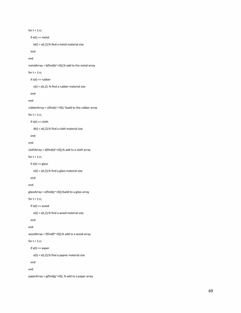
69
for t = 1:n;
if x(t) == metal
b(t) = x(t,2);% find a metal material size
end
end
metalArray = b(find(b~=0));% add to the metal array
for t = 1:n;
if x(t) == rubber
c(t) = x(t,2); % find a rubber material size
end
end
rubberArray = c(find(c~=0)); %add to the rubber array
for t = 1:n;
if x(t) == cloth
d(t) = x(t,2);% find a cloth material size
end
end
clothArray = d(find(d~=0));% add to a cloth array
for t = 1:n;
if x(t) == glass
e(t) = x(t,2);% find a glass material size
end
end
glassArray = e(find(e~=0));%add to a glass array
for t = 1:n;
if x(t) == wood
e(t) = x(t,2);% find a wood material size
end
end
woodArray = f(find(f~=0));% add to a wood array
for t = 1:n;
if x(t) == paper
e(t) = x(t,2);% find a paprer material size
end
end
paperArray = g(find(g~=0)); % add to a paper array

70
figure % create a histogram of the plastic material sizes
histogram(plasticArray)
title('Plastic')
xlabel('Centimeters')
ylabel('Quantity')
figure % create a divided plot of the material by there size
subplot(2,3,1);
histogram(metalArray)
title('Subplot 1: Metal')
xlabel('Centimeter')
ylabel('Quantity')
subplot(2,3,2);
histogram(rubberArray)
title('Subplot 2: Fabric')
xlabel('Centimeter')
ylabel('Quantity')
subplot(2,3,3);
histogram(clothArray)
title('Subplot 3: Organic')
xlabel('Centimeter')
ylabel('Quantity')
subplot(2,3,4)
histogram(glassArray)
title('Subplot 4: Glass')
xlabel('Centimeter')
ylabel('Quantity')
subplot(2,3,5)
histogram(woodArray)
title('Subplot 5: Wood')
xlabel('Centimeter')
ylabel('Quantity')
subplot(2,3,6)
histogram(paperArray)
title('Subplot 6: Paper')
xlabel('Centimeter')
ylabel('Quantity')

71
end
Top Related