


Languages
Pages
Legal


UNIVERSIDADE DE LISBOA
FACULDADE DE CIÊNCIAS
DEPARTAMENTO DE FÍSICA
Design of a Diffusion Phantom for Quality Control of
Spinal Cord DTI and EPI Distortion Improvement
Bruno Miguel de Brito Robalo
Mestrado Integrado em Engenharia Biomédica e B iofísica
Perf il em Radiações em Diagnóst ico e Terapia
Dissertação orientada por:
Dr. Bailiang Chen, INSERM U947 Imagerie Adaptative Diagnostique et Interventionnelle
Dr. Rita Nunes, Instituto de Biofísica e Engenharia Biomédica, Faculdade de Ciências da
Universidade de Lisboa
2016

If I have seen further it is by standing on the shoulders of giants.
- Sir Isaac Newton

i
ACKNOWLEDGEMENTS
First of all I want to express my deepest gratitude to all those who provided me the
opportunity to carry out this internship and work in an exceptional research team. I am very
thankful to INSERM and IADI for accepting me in their team and for funding my internship. I
also want to acknowledge the help and dedication of IADI director, Pr. Jacques Felblinger, who
promotes a spirit of fellowship, always encouraging the trainees to show and be confident in their
work.
To my supervisors Gabriella Hossu and Bailiang Chen, I want to say that I could not have
been luckier. Special thanks for your continuous guidance, patience, encouragement, and for
always being there when I needed support with work or the French administration. I had the
privilege of being supervised by two excellent professionals and I can say that I learned so much
and came to appreciate and pursue a career in research. Thank you for everything. During these
seven months I also had the privilege to learn from experts in MRI and programming, like Freddy
Odile, who was always very helpful and transmitted a great deal of knowledge. I also want to thank
my internal supervisor, Pr. Rita Nunes, for always being very helpful and giving valuable inputs for
my work.
I am grateful to the entire IADI team for providing the best work environment, especially
my office mates Maya, Antoine and Claire for always being so friendly, and for all the joyful times
that made work easier. I would also like to express my gratitude to my flatmate and friend Pedro
for all the good times, beers and cooking that made my stay in Nancy even more enjoyable.
Thanks to all my friends and colleagues, André, Carlos, Joana, Guimarães and Zé Nuno,
with whom explored some parts of Europe. Despite being abroad you made me feel home. My
gratitude to a special person, Mariana, for your words of encouragement, patience, friendship and
caring heart that always helped through rough times.
Lastly I would not forget my family, the most important people in my life. To my sisters
Evelyn and Vania, for your daily support and companionship. To my brother Samuel, for being a
role model to me. And finally to my parents José and Maria, for being to the two pillars of my life,
for all your support and for always believing in me no matter the circumstances.

ii
RESUMO
A imagem ponderada em difusão (DWI) é uma técnica de ressonância magnética (MR)
capaz de medir a magnitude da difusão de moléculas de água nos tecidos. A extensão desta técnica,
a imagem por tensor de difusão (DTI) utiliza gradientes aplicados ao longo de pelo menos seis
direções diferentes no espaço e deste modo é capaz de estimar também a principal direção de
difusão das moléculas de água nos tecidos. Consequentemente é possível obter informações sobre
a microestrutura de órgãos complexos como o cerebro e a medula espinhal. Estruturas como a
substância branca do cérebro e da medula espinhal, que são compostas por microfibras orientadas
de forma coerente, são os principais alvos de estudo de DTI, visto que esta técnica é mais sensível
a alterações que possam ocorrer na microestrutura de nervos ou neurónios.
Contudo, a medula espinhal é um órgão que apresenta vários desafios em MR,
especialmente em DTI. Em primeiro lugar, a medula espinhal tem uma dimensão relativamente
pequena quando comparada com outros órgãos e isto impõe dificuldades em termos da razão
sinal-ruído (SNR). Para além disso, as diferenças de suscetibilidade magnética entre diferentes tipos
de tecidos (medula espinhal, líquido cefalorraquidiano - LCR, osso, etc.) faz com que o campo
magnético seja menos homogéneo nessas regiões, o que por sua vez tem influência na origem de
artefactos e distorções da imagem. Outras complicações estão relacionadas com movimentos
fisiológicos (batimento cardíaco, respiração e fluxo do LCR). Em suma, estas complicações podem
resultar em estimativas erróneas dos parâmetros de DTI, o que pode influenciar o diagnóstico.
Com a evolução do hardware de MR e o desenvolvimento de novas sequências de impulsos,
e a implementação de técnicas de imagem rápidas fez com que o DTI fosse praticável em
ambiente clínico. A echo-planar imaging (EPI) é a principal sequência utilizada em DTI e permite
a obtenção de uma imagem em menos de cem milissegundos. Contudo, a EPI é muito sensível a
erros de fase e heterogeneidades do campo magnético que causam erros durante a reconstrução de
imagem, fazendo com que a presença de artefactos ghost, distorções geométricas e de intensidade
sejam frequentes. Deste modo, os passos necessários para a melhoria da qualidade de imagem não
podem ser ignorados. Isso pode ser conseguido durante a aquisição, modificando as sequências,
com a aplicação de técnicas como partial Fourier e parallel imaging que reduzem a quantidade de
linhas do espaço-k que são preenchidas, e consequentemente diminuem a acumulação de erros
relacionados com a EPI. Outra alternativa foca-se na melhoria da imagem após a aquisição, através

iii
da aplicação de métodos para correção de distorções e remoção de artefactos. Deste modo,
quando as dificuldades do DTI da medula espinhal são ultrapassadas, este torna-se numa
ferramenta de grande importância para o estudo de diversas patologias que afetam o sistema
nervoso central (CNS), como é o caso da esclerose múltipla (MS).
O principal objetivo deste estudo foi a otimização da sequência standard de DTI para a
medula espinhal utilizada em ambiente clínico, utilizando uma antena head-neck-spine
recentemente instalada. Para isso, foi construído um fantoma para simular as propriedades de
difusão da água na substância branca da medula espinhal. O fantoma é composto por fibras de
acrílico inseridas num tubo de plástico com dimensões semelhantes à medula espinhal.
Posteriormente, o tubo foi mergulhado em água de modo a que ocorra perfusão das fibras, sendo
assim possível simular algumas propriedades de difusão na medula espinhal.
O fantoma foi mantido na sala de MR a uma temperatura estável e foi submetido a várias
sessões de MR com o objetivo de determinar a configuração ideal da antena para a obtenção de
imagens da medula espinhal, bem como para a obtenção de imagens de DTI que iriam ser
utilizadas no pós-processamento. Problemas como a redução de ruído e minimização de artefactos
foram abordados durante a aquisição das imagens e durante o pós-processamento.
No pós-processamento, foi aplicado um método baseado na aquisição de duas imagens com
gradiente invertido para correção de distorções provocadas por diferenças de suscetibilidade do
campo magnético. Este método utiliza duas imagens de DTI obtidas nas mesmas condições e com
os mesmos parâmetros, com a exceção do gradiente de codificação de fase que apresentam
polaridades opostas, para calcular o mapa de deslocamento dos pixéis. Neste método, durante o
cálculo do mapa de deslocamento (DM) dos pixéis responsável pelas distorções, foram aplicadas
algumas inovações, nomeadamente um ajuste a uma curva sigmoide seguida por um ajuste a uma
superfície polinomial. O método modificado foi otimizado e comparado com o original em termos
de robustez na redução de distorções. Por fim, o mesmo protocolo de imagiologia e métodos de
melhoria de qualidade de imagem foram aplicados a imagens de voluntários saudáveis.
Os resultados demonstraram que o fantoma se manteve estável e as imagens obtidas foram
reprodutíveis durante o decorrer do estudo. Os parâmetros de DTI como a anisotropia fracionada
(FA) e o coeficiente de difusão aparente (ADC) foram calculados várias vezes e o seu valor foi
sempre dentro dos limites espectáveis. Para além disso, os mapas de codificação de cores FA
mostram que foi conseguida uma difusão anisotrópica nas fibras de acrílico, sendo que a difusão
ocorre predominantemente na direção paralela à orientação das fibras tal como acontece no caso

iv
da substância branca da medula espinhal. As imagens de tractografia também mostram que as
fibras são claramente distinguíveis das outras estruturas.
Nas imagens de DTI não corrigidas, existem distorções geométricas e de intensidade, sendo
que na região das fibras existem curvaturas e erros na estimativa da direção das fibras, fazendo com
que a imagem não seja uma representação fidedigna do fantoma físico. Após a aplicação, na sua
implementação original, do método de gradiente invertido para a correção de distorções, as regiões
com baixa intensidade de sinal continuam a apresentar curvaturas e são mal representadas.
Quando são aplicados o ajuste sigmoide e o ajuste à superfície polinomial, o método torna-se mais
eficiente, sendo capaz de minimizar as distorções em regiões de baixo sinal, bem como no resto da
imagem. Quando o mesmo método é aplicado às imagens de humanos, verifica-se que nas regiões
da imagem em que apenas existem distorções e não ocorrem artefactos ghost, o método de
correção é capaz de minimizar essas distorções. Contudo, na presença de artefactos que não sejam
apenas distorções, a correção é menos eficiente.
Em suma, o fantoma apresentado, apesar de ser uma simplificação da estrutura complexa da
medula espinhal, é um objeto estável que permitiu o estudo e otimização de uma sequência de
DTI para a medula espinhal, bem como o teste de métodos de pós-processamento para a melhoria
da qualidade de imagem.
Palavras-chave: Fantoma de difusão, imagem por tensor de difusão, medula espinhal,
distorções de suscetibilidade magnética, tractografia, substância branca.

v
ABSTRACT
Diffusion tensor imaging (DTI) is a magnetic resonance imaging (MRI) technique capable of
measuring the magnitude and direction of diffusion of water molecules within tissue and,
consequently, give an insight into the microstructure of complex organs such as the brain or the
spinal cord.
However, DTI of the spinal cord is arguably one of the most challenging applications of MRI
to the human body. Problems such as the small size of the spine, magnetic susceptibility differences
between surrounding tissues, local field inhomogeneities and bulk motion can cause image
deterioration, artifacts and distortions that ultimately result in erroneous estimations of DTI
parameters. With the evolution of coil technology, MR pulse sequences and the employment of
fast imaging techniques, DTI is becoming an important tool in clinical settings for the study of
pathologies that affect the central nervous system (CNS), such as multiple sclerosis (MS). However,
the steps necessary to improve image quality cannot be ignored: during acquisition with methods
such as partial Fourier and parallel imaging or after acquisition with post-processing methods.
The main goal of this work was to optimize the standard DTI sequence for the spine using a
newly installed coil. First, a diffusion phantom was built to simulate the diffusion properties of
white matter in the spine. The phantom is composed by acrylic fibers tightened inside a plastic tube
with dimensions similar to those of the spine and then perfused with water. Several scans were
performed on the phantom in order to determine the optimal coil configuration as well as to obtain
DTI images for post-processing. Here, a distortion correction method based on the reversed
gradient correction was applied to minimize susceptibly distortions. The correction method uses
two DTI datasets with opposite phase-encoding directions in order to estimate the pixel
displacement map (DM) that causes the intensity and geometric distortions. Here, some novelties
were applied to the reversed gradient method in the calculation of the DM, namely a sigmoid fit
followed by a polynomial surface fit. Finally, the same protocol and processing steps were applied
to images from healthy volunteers.
The results show that the phantom was stable and the obtained images displayed a good
reproducibility over time. DTI metrics such as FA (fractional anisotropy) and ADC (apparent
diffusion coefficient) were within the expected range and the fibers were clearly distinguishable in

vi
color maps and tractography images. The phantom allowed a continuous study and optimization of
the distortion correction method.
As expected, when no correction is applied, the DTI images present severe geometric and
intensity distortions. When the original reversed gradient correction is applied, regions of the image
with low signal, namely the fiber bundles, are still not accurately represented since the noise
influences the calculation of the DM. When the sigmoid and surface fit are added to the original
method, the distortions in the regions of low signal are minimized. Finally, when the method is
applied to human data, regions that are only affected by susceptibility distortions are corrected but
in the presence of ghost artifacts and motion, the method is less robust and cannot fully improve
the distorted regions.
In summary, the phantom is a simplification of the spinal cord, but nevertheless it is a reliable
object that allows the study and optimization of DTI protocols for the spine, as well as processing
methods for the improvement of image quality.
Key-words: Diffusion phantom, diffusion tensor imaging, spinal cord, magnetic susceptibility
distortion, fiber tractography, white matter.

vii
CONTENTS
ACKNOWLEDGEMENTS . . . . . . . . . . . . . . . . . . . . . . . . . . . . . . . i
RESUMO . . . . . . . . . . . . . . . . . . . . . . . . . . . . . . . . . . . . ii
ABSTRACT . . . . . . . . . . . . . . . . . . . . . . . . . . . . . . . . . . . . V
CONTENTS . . . . . . . . . . . . . . . . . . . . . . . . . . . . . . . . . . . vii
LIST OF TABLES . . . . . . . . . . . . . . . . . . . . . . . . . . . . . . . . . ix
LIST OF FIGURES . . . . . . . . . . . . . . . . . . . . . . . . . . . . . . . . . x
LIST OF ABBREVIATIONS . . . . . . . . . . . . . . . . . . . . . . . . . . . . . xiv
INTRODUCTION . . . . . . . . . . . . . . . . . . . . . . . . . . . . . . . . . 1
1 BACKGROUND . . . . . . . . . . . . . . . . . . . . . . . . . . . . . . . . 3
1.1 Diffusion Tensor Imaging . . . . . . . . . . . . . . . . . . . . . . . . . . 3
1.2 Echo-Planar Imaging (EPI) . . . . . . . . . . . . . . . . . . . . . . . . . . 6
1.3 K-space and Parallel Imaging . . . . . . . . . . . . . . . . . . . . . . . . . 7
1.4 Partial Fourier . . . . . . . . . . . . . . . . . . . . . . . . . . . . . . . 9
1.5 EPI susceptibility distortion . . . . . . . . . . . . . . . . . . . . . . . . 10
1.6 Distortion correction . . . . . . . . . . . . . . . . . . . . . . . . . . . 11
1.7 State-of-the-art of spinal cord DTI . . . . . . . . . . . . . . . . . . . . . . 12
2 MATERIALS & METHODS . . . . . . . . . . . . . . . . . . . . . . . . . . . . 18
2.1 Phantom Design . . . . . . . . . . . . . . . . . . . . . . . . . . . . . 18
2.2 Hardware . . . . . . . . . . . . . . . . . . . . . . . . . . . . . . . . 19
2.2.1 Coil Decoupling . . . . . . . . . . . . . . . . . . . . . . . . . . . 19
2.2.2 Data analysis . . . . . . . . . . . . . . . . . . . . . . . . . . . . 21
2.3 Phantom experiments . . . . . . . . . . . . . . . . . . . . . . . . . . . 22
2.3.1 Imaging protocol . . . . . . . . . . . . . . . . . . . . . . . . . . 22
2.3.2 Reconstruction . . . . . . . . . . . . . . . . . . . . . . . . . . . 23

viii
2.3.3 Distortion correction . . . . . . . . . . . . . . . . . . . . . . . . . 23
2.3.4 Data analysis . . . . . . . . . . . . . . . . . . . . . . . . . . . . 29
2.4 Healthy volunteer studies . . . . . . . . . . . . . . . . . . . . . . . . . 31
3 RESULTS . . . . . . . . . . . . . . . . . . . . . . . . . . . . . . . . . . . 32
3.1 Coil decoupling . . . . . . . . . . . . . . . . . . . . . . . . . . . . . 32
3.2 Distortion correction . . . . . . . . . . . . . . . . . . . . . . . . . . . 35
3.3 DTI metrics . . . . . . . . . . . . . . . . . . . . . . . . . . . . . . . 44
3.4 Healthy volunteer studies . . . . . . . . . . . . . . . . . . . . . . . . . 46
4 DISCUSSION . . . . . . . . . . . . . . . . . . . . . . . . . . . . . . . . . 48
5 CONCLUSION AND PERSPECTIVES . . . . . . . . . . . . . . . . . . . . . . . . 51
REFERENCES . . . . . . . . . . . . . . . . . . . . . . . . . . . . . . . . . . . 52
APPENDIX I . . . . . . . . . . . . . . . . . . . . . . . . . . . . . . . . . . . 57

ix
LIST OF TABLES
Table 2.1 - Coil configurations . . . . . . . . . . . . . . . . . . . . . . . . . . . 20
Table 2.2 – Organization of the data for the Wilcoxon test. Each column is a group and the
slice number is the criterion for the paired test. . . . . . . . . . . . . . . . 22
Table 2.3 - Organization of the data for the comparison of mutual information. . . . . . . . 30

x
LIST OF FIGURES
Figure 1.1 - Illustration of Spin Echo Diffusion Weighting Sequence with the 90° and 180° RF
pulses and diffusion gradients in gray (top). The middle section represents the
effect of the diffusion gradients on the phase of the molecules in the sample.
Finally, the bottom section represents the MR signal decay with time. a) – In
absence of motion the phase offset introduced by the first gradient is canceled by
the second. b) – In the presence of diffusion, the phase offset is not canceled after
the second gradient, producing an additional signal loss. Note: Image encoding
gradients omitted for simplicity purposes. Adapted from [6]. . . . . . . . . . 4
Figure 1.2 - a) Spin Echo DWI sequence with EPI readout. b) Corresponding k space
trajectory. Adapted from [2]. . . . . . . . . . . . . . . . . . . . . . . . 7
Figure 1.3 - a) Illustration of a fully sampled k-space and an under-sampled k-space that results
in an aliased image. b) Coil configuration and respective direction of acceleration.
Note that each coil is more or less sensitive to a specific volume of the object. In
parallel imaging each coil acquires an under-sampled k-space that results in an
aliased image. After application of SENSE or GRAPPA reconstruction a full FOV
image is obtained. Adapted from [12]. . . . . . . . . . . . . . . . . . . . 9
Figure 1.4 - a) ADC map of a sagittal slice of the cervical spinal cord. b) FA maps on of
different levels of the spinal cord. Note the higher intensities on the periphery,
corresponding to white mater, while grey matter (center) present lower anisotropy.
Adapted from [39]. . . . . . . . . . . . . . . . . . . . . . . . . . . . 15
Figure 1.5 – Sagittal T2 MRI image (A) in comparison with DT tractography images acquired
in two diagonally opposite planes. Three-dimensional tractography images
acquired in the medio–lateral and anterior–posterior (B and C) planes show the
disrupted fiber tracts [41]. . . . . . . . . . . . . . . . . . . . . . . . . 16
Figure 1.6 – A: MR imaging of a spinal cord involvement due to a solid state astrocytoma. FA
map and fiber tracking over b0 image show warped fibers around the tumor [42].
B: Selected axial T2-weighted image (left) of the cervical spinal cord of a MS
patient acquired at C3 level (the arrow indicates a hyperintense lesion). MD
(center) and FA (right) maps corresponding to the level of the T2 weighted image
[57].. ................................................................................................................................. 17
Figure 2.1 – Left – Bundle of acrylic-fibers tightened with (green) plastic cuffs inside a plastic
tube; One euro coin used for scale. Right – Final shape of the phantom; the fiber
bundle inside a bottle of water (1.5 liters). . . . . . . . . . . . . . . . . . 18
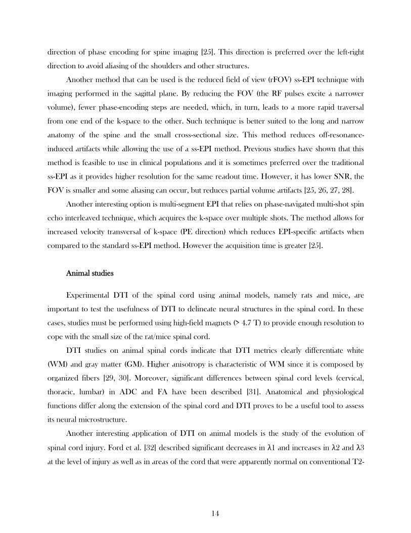
Figure 2.2 – A - Head-neck-spine coil. Sections A and B contain 6 groups of elements in the
posterior part. Section C corresponds to the face group, section D is the
“horseshoe” group and finally section E is the chest group. B – Coil configuration
superimposed to a sagittal slice of the head, neck and torso, showing the location
of each group relative to the body. . . . . . . . . . . . . . . . . . . . . 19
Figure 2.3 – Schematic representation of the algorithm used for distortion correction. Only the
most relevant steps are show for simplicity purposes. . . . . . . . . . . . . . 25

xi
Figure 2.4 – Matlab interface for EPI distortion correction and data analysis. The interface is
organized in 4 main panels: “1. Import Data from Archimed”; “2. Reversed
Gradient Correction”, “3. Corrected”; “4. Stats” . . . . . . . . . . . . . . . 29
Figure 3.1 - Signal-to-noise ratio in four channels when two coil configurations are used. The
red boxplot represents the coil configuration with segments 1-2 and with the chest
and face elements. The blue boxplot corresponds to the coil configuration with
segments 1-2 and without the face and chest elements. A: Channel 1; B: Channel
2; C: Channel 3; D: Channel 4. The boxplots represent values of SNR in 20 slices.
The Wilcoxon test was used for a pairwise comparison between the two coil
configurations. The asterisks represent the result of the test, *** (1.4 × 10⁻⁵
≤ p-
value ≤ 0.0013). . . . . . . . . . . . . . . . . . . . . . . . . . . . . 32
Figure 3.2 – Signal-to-noise ratio in seven channels for different coil configurations when the
chest and face elements are connected. The red boxplot corresponds to segments
1-2, the blue corresponds to 1-2-3 and the green corresponds to 1-2-3-4. The
boxplots represent values of SNR in 20 slices. The asterisks mark the result of the
Wilcoxon test performed pairwise between the three boxes. Red asterisk over the
blue plot is the result between the blue and red boxes; Red asterisk over the green
box is the result between the green and the red boxes; Blue asterisk over the green
box is the result between the green and blue boxes; * (p-value < 0.05); *** (p-value
< 0.001); When no asterisk are present it means that there is no significant
difference. . . . . . . . . . . . . . . . . . . . . . . . . . . . . . . 34
Figure 3.3 – Cumulative distribution function. A, B: CDFs of one slice in the I + image
before and after sigmoid fit, respectively. Each curve is represents the CDF from
one line of the image. Note the smoothness of the curves after the fitting. C: CDF
of one line (128) in the I+ image (in red) and in the I– image (in blue) before the
sigmoid fit; D: CDF of the same line after sigmoid fit. . . . . . . . . . . . . 35
Figure 3.4 - RMSE between the CDF+ and CDF- before and after sigmoid fit. A: Each point is
the RMSE between one CDF+ line and its corresponding CDF- line shown in
Figure 3.3. Note that one slice has 256 lines, therefore 256 values of RMSE are
calculated. B: Boxplot representation of the values shown in A. . . . . . . . . 36
Figure 3.5 – A – Preliminary corrected image used to generate a mask; B – Mask; C – Original
displacement map calculated from the CDF; D – DM with regions of low signal
intensity removed; E – DM fitted to a polynomial surface; F – Final displacement
map. . . . . . . . . . . . . . . . . . . . . . . . . . . . . . . . . . 37
Figure 3.6 – Top: A: DTI-EPI dataset with left-right phase encoding direction (blue arrow); B:
DTI-EPI dataset with right-left phase encoding direction (blue arrow), the + and –
symbolically indicate the PE direction; C: Distortion-free T2 FRFSE image.
Bottom: A: Contour (in magenta) of the DTI-EPI+ image superimposed to the T2
FRFSE; B: Contour of the DTI-EPI– image superimposed to the T2 FRFSE;
C: Contour of the T2 FRFSE superimposed to the respective image. Red arrows
indicate regions distortions. . . . . . . . . . . . . . . . . . . . . . . . 38
Figure 3.7 – Top: A: DTI-EPI after distortion correction using the original method with no
fitting; B: Result after distortion correction using only the sigmoid fit; C: Result
after when using both the sigmoid and surface fit in the correction method.

xii
Bottom: Contour of the images on the top superimposed to the distortion free T2
FRFSE images. Red arrows indicate regions of low SNR where the correction fails. 39
Figure 3.8 – Mutual information between the DTI-EPI and T2 FRFSE images. A: Boxplot
representation of the MI before and after distortion correction with different
methods. B-G: Pairwise comparison between the boxplots; The Wilcoxon test was
used; the asterisk represent the result of the test, ** (0.015 ≤ p-value ≤ 0.022). No
asterisks are shown when the p-value > 0.05. . . . . . . . . . . . . . . . . 40
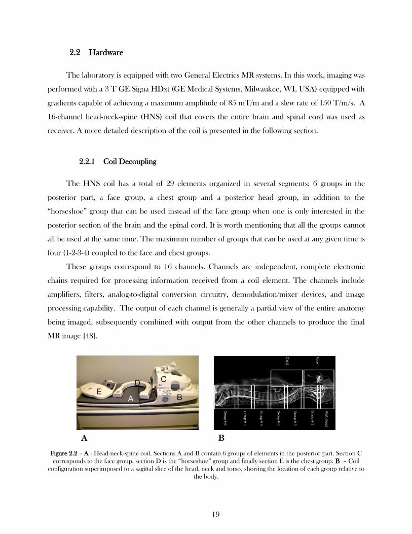
Figure 3.9 – Fiber tracts computed with the STT technique before distortion correction. Red
arrow indicates a curvature in the fiber tracts due to distortion. Red and yellow
boxes indicate the regions that were amplified and shown in the bottom images.
The left image shows the seed ROI where the fiber tracking begins. The right
image shows a region where errors in fiber tracking occur.. . . . . . . . . . . 41
Figure 3.10 – Fiber tracts computed with the STT technique correction without sigmoid or
surface fit. Red arrow indicates a curvature in the fiber tracts due to distortion. Red
and yellow boxes indicate the regions that were amplified and shown in the bottom
images. The left image shows the seed ROI where the fiber tracking begins. The
right image shows a region where errors in fiber tracking occurs. . . . . . . . . 42
Figure 3.11 – Fiber tracts computed with the STT technique after correction with the sigmoid
fit alone. Red arrow indicates a curvature in the fiber tracts due to distortion. Red
and yellow boxes indicate the regions that were amplified and shown in the bottom
images. The left image shows the seed ROI were the fiber tracking begins. The
right image shows a region were errors in fiber tracking occurs. . . . . . . . . 43
Figure 3.12 – Fiber tracts computed with the STT technique after correction using both the
sigmoid and surface fit. The curvature present in figures is minimized. Red and
yellow boxes indicate the regions that were amplified and shown in the bottom
images. The left image shows the seed ROI were the fiber tracking begins. The
right image shows a region were errors in fiber tracking occurred in the previous
case. . . . . . . . . . . . . . . . . . . . . . . . . . . . . . . . . . 44
Figure 3.13 – A: FA maps of ten slices. The fiber bundle presents higher values. B: Color
coded FA map. The colors are defined by the direction of the main eigenvector
and the amplitude is weighted by FA. Note the color code given by the arrow
system. Diffusion in the up-down direction is represented in red; Left-right is
represented in green, and finally inwards-outwards of the plane is represented by
blue. C: ADC maps. Regions congaing free water have higher values. D: FA and
ADC values in the fiber bundle over a period of 4 months. The Mann-Wallis test
shoes now significant difference over time; p-value > 0.6. . . . . . . . . . . . 45
Figure 3.14 – Images from healthy volunteers before correction. Top: A: Dataset with left-
right phase encoding direction (blue arrow); B: Dataset with right-left phase
encoding direction (blue arrow), the + and – symbolically indicate the PE
direction; C: Distortion-free T2 FRFSE image. Bottom: A: Contour (in magenta)
of the DTI-EPI + image superimposed to the T2 FRFSE; B: Contour of the DTI-
EPI– image superimposed to the T2 FRFSE; C: Contour of the T2 FRFSE
superimposed to the respective image. Red arrows indicate distortions. Yellow
arrows indicate ghost artifact. . . . . . . . . . . . . . . . . . . . . . . . 46

xiii
Figure 3.15 – Images from healthy volunteers after correction. Top A: Post correction using
the original method with no fitting; B: Result after distortion correction using only
the sigmoid fit; C: Result after using both the sigmoid and surface fit in the
correction method. Bottom: Contour of the images on the top superimposed to
the distortion free T2 FRFSE images. Red arrows indicate regions where the
correction fails. . . . . . . . . . . . . . . . . . . . . . . . . . . . . 47

xiv
LIST OF ABBREVIATIONS
2D . . . . . . . . . . . . . . . . . . . . . . . . . . . . . . . . . two-dimensional
ADC . . . . . . . . . . . . . . . . . . . . . . . . . . . apparent diffusion coefficient
AP . . . . . . . . . . . . . . . . . . . . . . . . . . . . . . . . . anterior-posterior
CDF . . . . . . . . . . . . . . . . . . . . . . . . cumulative distribution function
CNS . . . . . . . . . . . . . . . . . . . . . . . . . . . . . central nervous system
CSF . . . . . . . . . . . . . . . . . . . . . . . . . . . . . . . cerebrospinal fluid
DM . . . . . . . . . . . . . . . . . . . . . . . . . . . . . . . displacement map
DTI . . . . . . . . . . . . . . . . . . . . . . . . . . . . . diffusion tensor imaging
DWI . . . . . . . . . . . . . . . . . . . . . . . . . . . . diffusion weighted imaging
EPI . . . . . . . . . . . . . . . . . . . . . . . . . . . . . . echo-planar imaging
FA . . . . . . . . . . . . . . . . . . . . . . . . . . . . . . . fractional anisotropy
FE . . . . . . . . . . . . . . . . . . . . . . . . . . . . . . . . frequency encoding
FID . . . . . . . . . . . . . . . . . . . . . . . . . . . . . . free induction decay
FOV . . . . . . . . . . . . . . . . . . . . . . . . . . . . . . . . . . field-of-view
FRFSE . . . . . . . . . . . . . . . . . . . . . . . . . . . fast recovery fast spin echo
FSPGR . . . . . . . . . . . . . . . . . . . . . . . . . . . fast spoiled gradient echo
FT . . . . . . . . . . . . . . . . . . . . . . . . . . . . . . . . Fourier transform
GM . . . . . . . . . . . . . . . . . . . . . . . . . . . . . . . . . . gray matter
GRAPPA . . . . . . . . . . . . . . generalized autocalibrating partially parallel aquisition
HARDI . . . . . . . . . . . . . . . . . . . . high angular resolution diffusion imaging
HNS . . . . . . . . . . . . . . . . . . . . . . . . . . . . . . . . head-neck-spine
IADI . . . . . . . . . . . . . . . . Imagerie Adaptative Diagnostique et Interventionnelle
MI . . . . . . . . . . . . . . . . . . . . . . . . . . . . . . . . mutual information
MR . . . . . . . . . . . . . . . . . . . . . . . . . . . . . . . magnetic resonance
MRI . . . . . . . . . . . . . . . . . . . . . . . . . . . magnetic resonance imaging
NEX . . . . . . . . . . . . . . . . . . . . . . . . . . . . . . number of excitations
PE . . . . . . . . . . . . . . . . . . . . . . . . . . . . . . . . . phase encoding
PGSE . . . . . . . . . . . . . . . . . . . . . . . . . . . pulsed gradient spin echo

xv
PSF . . . . . . . . . . . . . . . . . . . . . . . . . . . . . . point spread function
QBI . . . . . . . . . . . . . . . . . . . . . . . . . . . . . . . . . Q-ball imaging
ReLSEP . . . . . . . . . . . . . . . . . . . Registre Lorraine de la Sclerose en Plaque
RF . . . . . . . . . . . . . . . . . . . . . . . . . . . . . . . . . radio frequency
rFOV . . . . . . . . . . . . . . . . . . . . . . . . . . . . . reduced field of view
SCI . . . . . . . . . . . . . . . . . . . . . . . . . . . . . . . . spinal cord injury
SE . . . . . . . . . . . . . . . . . . . . . . . . . . . . . . . . . . . . spin echo
SENSE . . . . . . . . . . . . . . . . . . . . . . . . . . . . . . sensitivity encoding
SNR . . . . . . . . . . . . . . . . . . . . . . . . . . . . . . . signal-to-noise ratio
ss-EP . . . . . . . . . . . . . . . . . . . . . . . . . . single shot echo-planar imaging
STT . . . . . . . . . . . . . . . . . . . . . . . . . . streamline tracking technique
TE . . . . . . . . . . . . . . . . . . . . . . . . . . . . . . . . . . . echo time
TR . . . . . . . . . . . . . . . . . . . . . . . . . . . . . . . . . repetition time
WM . . . . . . . . . . . . . . . . . . . . . . . . . . . . . . . . . . white matter

1
INTRODUCTION
Diffusion-weighted imaging (DWI) and its extension diffusion tensor imaging (DTI) are
magnetic resonance (MR) techniques capable of measuring the magnitude of diffusion of water
molecules within tissues. With DTI it is also possible to measure the direction of diffusion, and
consequently the estimation of tissue microstructure. Spinal cord DTI is one of the most
challenging applications of MR imaging to the human body. Difficulties such as the relative small
size of the spine, magnetic susceptibility differences between surrounding tissues (bone, cerebro-
spinal fluid - CSF, spinal cord), local field inhomogeneities and bulk motion are among the factors
that cause image deterioration, artifacts and distortions.
Advancements in software and hardware have allowed for the development of more complex
MR pulse sequences, designed specifically to overcome these difficulties. When its inherent
imaging challenges are overcome, DTI can be a valuable tool to assess several spinal cord
pathologies, which affect both anatomy and physiology, such as multiple sclerosis (MS).
DTI sequences usually employ an echo planar imaging (EPI) readout to avoid macroscopic
motion artifacts and reduce the readout time. This can also be coupled with parallel imaging and
partial Fourier to further decrease the readout, making DTI feasible in clinical settings.
Furthermore, parallel imaging and partial Fourier in EPI reduce the echo train length (ETL) and
therefore reduce EPI specific artifacts. However, implementation of parallel imaging in the spinal
cord remains challenging, due the geometric arrangement of the coils that is usually in conflict with
the preferred phase encoding (PE) direction. These fast imaging capabilities always come with a
cost in image quality. EPI is very sensitive to field inhomogeneities that cause image distortion and
this is aggravated in the spinal cord. This can be minimized with post-processing algorithms that
estimate the distortion field and use it to obtain the undistorted image.
The IADI laboratory where this work was carried out is part of a network that aims to
improve knowledge of multiple sclerosis (MS) and to advance research on prevention and
treatment. A registry (ReLSEP - Registre Lorraine de la Sclerose en Plaque) was opened and since
2009, 180-250 new cases are being included into the registry each year. Several clinical research
protocols have been initiated in order to perform MRI on a portion of the network patients,
including spinal cord DTI since the spine can also be affected by MS.

2
In this manuscript, the theoretical background necessary to understand this work is
introduced in Chap. 1. Concepts such as DTI, parallel imaging, partial Fourier, EPI and
susceptibility distortions are explained (Chap. 1.1 to Chap. 1.6). A state-of-the-art of spinal cord
DTI is also disclosed in Chap. 1.7.
The aim of this study was to optimize the standard DTI sequence for the spinal cord using
the newly installed head-neck-spine (HNS) coil with a focus on artifact and distortion reduction.
For this purpose, a phantom was built to simulate the diffusion properties in the spinal cord
(Chap. 2.1). Problems such as field inhomogeneity, noise and artifact reduction were addressed
(Chap. 2.3). Optimization of the sequence was performed during acquisition by studying methods
such as parallel imaging and partial Fourier (Chap. 2.4.2) and with post processing methods to deal
with distortions (Chap 2.4.3). Finally a pilot healthy volunteer study was conducted to ensure the
robustness of the implemented optimization steps and to evaluate the reproducibility of the
measured DTI parameters (Chap. 2.5).
The results of these studies are presented in Chap. 3 and a discussed in chapter 4. A general
conclusion is provided in chapter 5.

3
1 BACKGROUND
1.1 Diffusion Tensor Imaging
The free induction decay (FID) MR signal can be made sensitive to the movement of water
molecules (Brownian motion) within the tissue, providing contrast which reflects their molecular
displacement on a sub-voxel scale.
It was however, Stejskal and Tanner that provided a detailed description of a DW MR
sequence in 1964 [1]. Briefly, the pulsed gradient spin echo (PGSE) sequence is based on the
standard SE sequence with an additional pair of identical diffusion weighting gradients placed
symmetrically on both sides of the 180° RF pulse, which makes the sequence sensitive to the
diffusion of water molecules. A detailed explanation of MRI and the standard SE sequence is
beyond the scope of this work but it can be found in references [2, 3]. As shown in Figure 1.1, the
first diffusion gradient, before the 180° pulse, adds an additional phase offset dependent on each
molecule’s position. After the 180° refocusing pulse, if the molecule’s position did not change, the
second diffusion gradient will reverse the phase offset. In this case, the only signal loss that will be
measured is due to the T2 relaxation process. However, if there is motion due to diffusion in the
direction of the applied gradients, the individual positions will differ between the application of the
first and second diffusion gradients. Therefore, the second gradient will not cancel the phase offset
caused by the first. This will result in an additional loss in amplitude of the signal that is
independent of the T2 relaxation.
The degree of signal loss can be quantified by the following equation [1, 4, 5]:
S = S0 exp(−bD) (1.1)
Here, S is the signal intensity, S0 the signal intensity when no diffusion gradients are applied, b
is the diffusion sensitizing factor (b-value) and D the apparent diffusion coefficient (ADC), usually
expressed in mm2
/s. The b-value (s/mm2
) carries the information about the diffusion encoding
gradients and can be expressed as:
b = γ2G2δ2 (Δ −δ
3 ) (1.2)

4
Here, 𝛾 is the gyromagnetic ratio of the nucleus, G the gradient amplitude, 𝛿 the duration of
the gradient and 𝛥 the time interval between the applications of the two gradients.
Figure 1.1 - Illustration of Spin Echo Diffusion Weighting Sequence with the 90° and 180° RF pulses and diffusion
gradients in gray (top). The middle section represents the effect of the diffusion gradients on the phase of the molecules
in the sample. Finally, the bottom section represents the MR signal decay with time. a) – In absence of motion the
phase offset introduced by the first gradient is cancelled by the second. b) – In the presence of diffusion, the phase
offset is not cancelled after the second gradient, producing an additional signal loss. Note: Image encoding gradients
omitted for simplicity purposes. Adapted from [6].
By performing at least two experiments with different b-values, b1 and b2 (usually
b1 = 0 smm-2), one can extract the ADC of the sample by means of:
𝐷 = −1
𝑏1− 𝑏2𝑙𝑛 (
𝑆(𝑏1)
𝑆(𝑏2) ) (1.3)
Where S (b1) and S (b2) represent…
With this sequence, a contrast can already be achieved and ADC maps can be generated.
In pure water, the molecules move randomly without any predominant diffusion direction,
therefore there is an isotropic diffusion. In biological tissues, such as gray matter, despite being
practically isotropic, diffusion is hindered by macromolecules and cell structures. In white matter of
the brain for example, motion of water parallel to axon fibers is facilitated while motion in the
perpendicular direction is restricted, leading to an anisotropic diffusion [7].
In order to estimate directionality, the concept of diffusion tensor was introduced by Basser
et al. [8]. Here, Equation (1.1) can be extended to reflect the complete 3-dimensional diffusion co-
variance matrix, where D is measured in at least 6 directions (in addition to a b0 image) and fitted
by a 3×3 symmetric matrix. The matrix is also positive and definite.

5
D = [
Dxx Dxy DxzDyx Dyy DyzDzx Dzy Dzz
] (1.4)
By diagonalization of the tensor we obtain three eigenvectors 𝑒1 , 𝑒2 , 𝑒3 and their
corresponding eigenvalues 𝜆1 ≥ 𝜆2 ≥ 𝜆3. The first eigenvector can be interpreted as the principal
diffusion direction and 𝜆1 its amplitude. This eigenvector is assumed to represent the main
direction of the fibers in that voxel [9]. The first eigenvalue is also known as axial diffusivity (parallel
to the fibers) while the mean of 𝜆2 and 𝜆3 represent radial diffusivity (perpendicular to the fibers).
Given these parameters, other metrics can be computed:
ADC = λ1+ λ2+ λ3
3 (1.5)
The fractional anisotropy (FA) that represents the degree of diffusion anisotropy in each
voxel (0, isotropic; 1, anisotropic) is derived as:
FA = √3
2 √(λ1− ADC)2+ (λ2 − ADC)2+ (λ3 − ADC)2
√λ12+ λ2
2+ λ32
(1.6)
In order to accurately estimate diffusion metrics and fiber orientations, DTI sequences
acquiring more than six images corresponding to non-coplanar diffusion directions are required. In
this case, the 3×3 tensor matrix is obtained by linear least-square fit as explained in detail by
Kingsley [10]. Using matrix algebra, this model can be summarized by the following equation:
𝑌 = 𝐻𝑑 (1.7)
Here, d is the unknown six-element column vector representing the tensor matrix,
𝑑 = [Dxx, Dyy, Dzz, Dxy, Dxz, Dyz]𝑇 (1.8)
H is a large M x 6 matrix, containing the gradient direction coefficients. M is the number of
gradient directions and each gradient direction gi is represented by a vector (𝐺𝑥𝑖 , 𝐺𝑦𝑖 , 𝐺𝑧𝑖),

6
𝐻 =
(
𝐺𝑥12 𝐺𝑦1
2 𝐺𝑧12 2𝐺𝑥1𝐺𝑦1 2𝐺𝑥1𝐺𝑧1 2𝐺𝑦1𝐺𝑧1
𝐺𝑥22 𝐺𝑦2
2 𝐺𝑧22 2𝐺𝑥2𝐺𝑦2 𝐺𝑥2𝐺𝑧2 2𝐺𝑦22𝐺𝑧2
⋮ ⋮ ⋮ ⋮ ⋮ ⋮𝐺𝑥M2 𝐺𝑦1
2 𝐺M12 2𝐺𝑥M𝐺𝑦M 2𝐺𝑥M𝐺𝑧M 2𝐺𝑦M2𝐺𝑧M)
(1.9)
Lastly, the left side of Equation (1.7) is defined as:
𝑌 = (ln
𝑆0𝑆1
𝑏, ln
𝑆0𝑆2
𝑏, … , ln
𝑆0𝑆M
𝑏)𝑇
(1.10)
Note that apart from the signal intensities for each gradient direction (𝑆𝑖), another
measurement with b = 0 smm-2 is required (𝑆0). In equation (1.7) the only unknown term is d. For
six gradient directions (M = 6), the equation has an exact solution. When more than six diffusion
gradient direction are used, an approximate solution can be obtained by linear least square fit [10].
1.2 Echo-Planar Imaging (EPI)
In DTI, one measures microscopic motion of water molecules due to diffusion while
simultaneously trying to avoid macroscopic motion due to respiration and other physiological
mechanisms, meaning that a fast imaging capability is required.
Echo-planar imaging is one of the fastest MR imaging techniques, capable of acquiring an
image in less than 100 ms [2, 11]. In conventional imaging, one line of imaging data (one line in k-
space or one phase-encoding step) is collected within each repetition time (TR). The pulse
sequence is then repeated for multiple TR periods until all phase-encoding steps are collected and
k-space is filled. Therefore, the imaging time is equal to the product of the TR and the number of
phase-encoding steps. In single shot EPI, multiple lines of imaging data are acquired after a single
RF excitation. Like a conventional SE sequence, a SE-EPI sequence begins with 90° and 180° RF
pulses. However, after the 180° RF pulse, the frequency-encoding gradient oscillates rapidly from a
positive to a negative amplitude, forming an echo train (Figure 1.2 a). Each echo is phase encoded
differently by phase-encoding (PE) blips on the PE axis. Each oscillation of the frequency-encoding
gradient corresponds to one line of imaging data in k space, and each blip corresponds to a
transition from one line to the next in k-space as illustrated in references [2, 12].

7
With this sequence, acquisition times of 100 ms/slice can be achieved. However, EPI suffers
from several artifacts linked to: sensitivity to magnetic susceptibility, which can be reduced by
acquiring a shorter echo train (parallel imaging and/or partial Fourier); gradient imperfections
(particularly induced currents) which perturb spatial encoding, leading to ghost images [12].
Figure 1.2 - a) Spin Echo DWI sequence with EPI readout. b) Corresponding k space trajectory. Adapted from [2].
1.3 K-space and Parallel Imaging
In MRI, information about the image is collected in k-space which contains spatial frequency
information and is related to the actual image through the Fourier transform (FT). The spacing
between k-space points is inversely proportional to the field-of-view (FOV) in that direction. For
example, decreasing the spacing in y-direction of k-space will result in increase of FOV in the same
direction in the image domain. The highest frequency collected in k-space (kx,max or ky,max) is
inversely proportional to the image resolution, or spacing between points in the image domain (Δx
or Δy, respectively). The FOV and resolution can be manipulated by changing the number of
points acquired in k-space, the spacing between these points and the k-space spanned by these
points [13].
In conventional sequences, k-space data are acquired line by line in order to fill the entire
grid of points before the inverse FT is applied to obtain the final image. The kx direction is the
frequency-encoding direction and the ky direction is the phase-encoding direction. In general, the
acquisition time is proportional to the time necessary to read one line (repetition time, TR)
multiplied by the number of lines (phase-encoding steps) [13].

8
One possibility to decrease acquisition time is to reduce the amount of k-space data collected
by under-sampling in y-direction, in other words, by increasing the spacing between the lines. In
this case the original resolution is maintained because the highest frequencies are also collected but
the FOV in y-direction is reduced which will result in aliasing (Figure 1.3 a). The reason for this is
that as the k-space data are under-sampled, a high-frequency originating from one part of the object
is indistinguishable from a low frequency signal originating from another part of the object and the
two locations will overlap in the image (aliasing). The spacing between points in k-space needs to be
small enough so that the frequencies from different locations within the object can be distinguished
from one another. The FOV should be at least as large as the image size of the object. This is
known as the Nyquist criteria [14].
In parallel imaging the acquisition is accelerated by collecting fewer phase-encoding lines in k-
space (under-sampling), which will result in aliased images that must be corrected for clinical
purposes. There are several parallel imaging methods but they are all based on the same principles
[13]:
1. K-space data are under-sampled in the phase-encoding direction to reduce the scan time.
The acceleration factor R, is inversely proportional to the number of lines acquired. If the
fully sampled image is composed by 80 lines in k-space and the acquisition is accelerated by
a factor of R = 2, the resulting k-space will only be composed of 40 lines.
2. Data are acquired using an array of independent receiver channels instead of using a large
homogeneous volume receiver coil. Each channel is more sensitive to the specific volume
of tissue nearest to the coil, which means that the channels provide additional spatial
information for image reconstruction. It is important that the PE direction (the direction
along the acceleration will be performed) is in accordance with the coil configuration. In
other words, the coil geometry must be in such manner that distinct channels have different
sensitivities in the PE direction (Figure 1.3 b).
3. A special algorithm, which requires the knowledge of individual coil sensitivities, is used to
combine the under-sampled data from each of the receiver coils into the unalisaed
reconstructed image with the full FOV.
Note that parallel imaging is not a pulse sequence but instead a reconstruction algorithm that
can be used to reconstruct under-sampled data from any type of pulse sequences. These algorithms
can be grouped into two categories: algorithms that act on the aliased images of each coil in the
image domain (e.g. SENSE – SENSitivity Encoding) [13, 15] and algorithms that act in the under-

9
sampled k-space and estimate the missing lines of data (e.g. GRAPPA - Generalized
Autocalibrating Partially Parallel Acquisitions) [13, 16].
Figure 1.3 - a) Illustration of a fully sampled k-space and an under-sampled k-space that results in an aliased image. b)
Coil configuration and respective direction of acceleration. Note that each coil is more or less sensitive to a specific
volume of the object. In parallel imaging each coil acquires an under-sampled k-space that results in an aliased image.
After application of SENSE or GRAPPA reconstruction a full FOV image is obtained. Adapted from [13].
1.4 Partial Fourier
Partial Fourier takes advantage of the conjugate symmetry properties of the Fourier
transform. In theory, MRI images represent the spin density as a function of position, hence should
be real valued. Since real functions have conjugate symmetry in frequency space (k-space) an image
can be reconstructed by acquiring only part of the data (half or more) in the frequency domain.
The uncollected data can be synthetized by reflecting conjugate data across the origin of the k-
space. Unfortunately there are many sources of phase errors that cause the real-valued assumption
to be violated. These include variations in resonance frequency, flow and motion. As a result,
partial Fourier reconstruction always requires some type of phase correction that allows a real
image to be reconstructed [17].
The simplest method to reconstruct a partial k-space dataset is to simply fill the uncollected
data with zeros, followed by inverse 2D FT and display the magnitude. This works well if the
fraction of k-space collected is close to 1 and works poorly when this fraction approaches 0.5. The
result is significant blurring in the phase-encoding direction. The reason for the blurring can be
identified by considering the partial dataset to be a product of the full k-space multiplied by a

10
weighting function (a step function). In order to correct for the blurring, the missing uncollected
data must be synthetized by exploring the k-space symmetry. However, phase correction must not
be skipped [17].
Methods such as Homodyne reconstruction and Iterative partial k-space reconstruction apply
phase correction and then the conjugate symmetry principle in one or several steps, respectively
[17].
1.5 EPI susceptibility distortion
Magnetic susceptibility (χ) is a property of material that characterizes the degree to which the
material interacts with the external magnetic field. There is microscopic variation of the magnetic
field near the interface between substances with different magnetic susceptibility. In the human
brain, large variation of the B0 field can be observed near the sinuses which are the interface of air
and water (brain tissue) as well as in the spinal cord close to bone-CSF interfaces and in regions of
the thoracic spine due to the proximity of the lungs. Since the field inhomogeneity is proportional
to susceptibility inhomogeneity and field strength, the higher the field strength, the worse the
artifacts are [18]:
𝑀𝑖𝑛𝑑𝑢𝑐𝑒𝑑 = 𝜒𝐵0 (1.11)
Two kinds of artifacts can be caused by susceptibility: local signal loss due to dephasing
within the voxel (intravoxel dephasing) and geometric image distortion (voxel shift). The MR signal
in the presence of field inhomogeneity 𝛥𝐵0(𝑥, 𝑦) can be expressed by [18]:
𝑠(𝑡) = ∬𝑚(𝑥, 𝑦)exp [−𝑖2𝜋(𝑘𝑥(𝑡)𝑥 + 𝑘𝑦(𝑡)𝑦) ]exp [𝑖𝛾𝛥𝐵0(𝑥, 𝑦)𝑡] 𝑑𝑥𝑑𝑦 (1.12)
The second exponential term is the phase error, which is dependent on the field
inhomogeneity. According to the time-shift property of the Fourier transform, after the FT, the
phase error becomes the pixel shift in the image space. That is how geometric distortion produced
in the MR image is related with the existence of field inhomogeneity due to susceptibility
differences. The effect of 𝛥𝐵0 on the image also depends on the trajectory used to fill the k-space.

11
For a conventional sequence, after the RF excitation in each TR, one line of k-space is
measured. If there is some phase error due to susceptibility difference, it will only occur
immediately after the RF excitation and reset to zero after the relaxation (assuming a full relaxation
after each TR). Therefore, the phase errors are minimal for the conventional SE sequence.
However, the scenario is different for single-shot EPI where the whole k-space is measured (single-
shot). The phase error accumulates over the acquisition process. That is the reason that EPI is
much more affected by susceptibility distortion. Since the time interval between two lines in the
phase-encoding direction is much longer than in the frequency-encoding direction, the geometric
distortions is predominantly in the PE direction. Therefore, the phase error in the frequency
direction is usually neglected. Equation (1.12) can be written in the form of [18]:
𝑠(𝑘𝑥, 𝑘𝑦) ≈ ∬𝑚(𝑥, 𝑦). exp [−𝑖2𝜋{𝑘𝑥. 𝑥 + 𝑘𝑦[𝑦 + 𝛾𝛥𝐵0(𝑥, 𝑦)𝛥𝑇
𝛥𝑘𝑦]}] 𝑑𝑥𝑑𝑦 (1.13)
After the Fourier transform, the pixel displacement in the image space can be quantified as:
𝛥𝑦 = 𝛾𝛥𝐵0(𝑥, 𝑦)𝛥𝑇 (1.14)
Where 𝛾 is the gyromagnetic ratio of the nucleus, 𝛥𝐵0 is the field inhomogeneity and 𝛥𝑇 the
time between successive echoes in the EPI echo train.
1.6 Distortion correction
There are several methods for the improvement of image quality. These algorithms can be
categorized into two classes: improvement in the data collecting process and improvement in the
post-acquisition process for distortion correction. In the first case the aim is to reduce the phase
error accumulation by reducing the amount of k-space lines acquired after each excitation. This can
be achieved with parallel imaging. On the other hand, there are post-processing methods that
reduce the susceptibility distortions.
The most intuitive and widely used method is field map correction. This method first measures
the field inhomogeneity maps and calculates the voxel shift map based on the field inhomogeneity map
[19]. However, the field map method requires an additional acquisition to obtain the field
inhomogeneity information. It is difficult to accurately match the field map with EPI image pixel-by-
pixel. The commonly used smoothing process further limits its accuracy [18]. Furthermore, when the

12
phase errors overcome a certain limit, phase wrapping will occur, compromising the effectiveness of the
method. Another approach is the point spread function (PSF) [20]. In this method, an additional
spin-warp PE gradient, which encodes the same spatial information as the EPI PE gradient, is
added to the original EPI sequence. After 3D inverse fast Fourier transformation, the reconstructed
PSFs are represented along the correlation (or diagonal) line in the spin-warp (or non-distorted)
and EPI (or distorted) PE coordinates. Any distortion in the image is reflected in a deviation of the
PSFs from the diagonal line along the EPI PE coordinates versus the spin-warp PE coordinates,
and thus this deviation of the PSFs allows the accurate calculation of distortions. This method has
the potential to provide robust solutions to the distortion problem in regions of high or low field
inhomogeneity and allow the correction of both geometric and intensity distortions. However, it is not
only more computationally expensive but also has longer acquisition time (#PE lines × EPI acquisition
time).
Another approach is the reversed gradient method [21, 22] that estimates the distortion field from
two EPI images with opposite PE direction and uses it to calculate the undistorted image. The method
is described in detail in the Materials & Methods section.
1.7 State-of-the-art of spinal cord DTI
DTI itself is well established and has its main applications in the brain, but much less so in
the spinal cord. This part of the central nervous system is a more challenging structure to study. In
clinical in vivo settings, where acquisition time should be kept as short as possible, these difficulties
increase along with the demands on hardware and software performance.
Technical challenges
The small size of the spine and surrounding structures require smaller voxel sizes (higher
matrices) for adequate spatial resolution, which will decrease the SNR [23]. The spinal cord is a
relatively small structure with approximately 45 cm in length in the adult male, with the largest
cross-sectional area in the lower cervical (38 mm circumference) and lumbar regions (35 mm). This
means that a sagittal acquisition is usually necessary to obtain sufficient coverage in a reasonable
scan time [7]. Nonetheless, axial slices can also be obtained.
Some spinal regions present even greater challenges arising from magnetic susceptibility
artifacts due to surrounding bony structures, such as at the cervicothoracic junction, for example.

13
This results in off-resonance–related artifacts and limits the usable readout duration [24].
Moreover, the bone–CSF and air-bone interfaces in the thoracic region, given the proximity of the
pulmonary parenchyma, lead to local field inhomogeneity due to susceptibility differences between
tissues, which in turn creates off-resonance induced artifacts in the images. Generally this results in
geometric distortions. Furthermore, when moving to higher magnetic fields, these challenges are
aggravated as the absolute size of the field perturbations increase with B0. The naturally very-curved
shape of the spine can also create field distortions [24].
Another problem arises from physiological motion, from cardiac and respiratory cycles, as
well as CSF pulsation that results in nonlinear phase errors and shifts/dispersions of k-space when
these motions occur during the diffusion encoding gradients and the phase encoding direction is
anterior-posterior (AP), resulting in ghosting artifacts and erroneous estimations of DTI metrics
[25, 26]. Some of these problems can be reduced by cardiac and/or respiratory gating but the
pulsatile motion of CSF remains difficult to overcome and can lead to significant artifacts since they
occur independently. With improvement of software and hardware technology, some of these
challenges can be minimized, as described below.
Imaging protocols
A fast imaging capability is crucial in order to avoid the effects of macroscopic motion (e.g.
respiration). EPI based sequences put enormous demands on hardware capabilities. The
requirements for gradient strength, rise time and duty cycle are markedly increased because all of k-
space is traversed following a single RF excitation by using a rapidly oscillating frequency-encoding
gradient. Modern clinical scanners are usually equipped with gradient strengths of 40 - 70 mT/s and
slew rates of 200 T/m/s. In EPI, the full capabilities of the gradients are made use of [12].
The most commonly used technique for DTI is the SE single-shot EPI (ss-EPI). As all data is
acquired within a single shot, with this method magnitude images do not suffer from ghosting
artifact and higher resolutions can be obtained by acquiring a longer echo train, or by using a multi-
shot method. However, image distortions may still persist in regions of inhomogeneous magnetic
susceptibility. Distortions can be reduced using parallel imaging in such EPI sequences because the
readout duration is reduced, avoiding cumulative EPI errors. Successful implementation and
application of parallel imaging in the spine is limited primarily because of the geometric
arrangements of spine array coils, which is often in conflict with the preferred anterior-posterior
14
direction of phase encoding for spine imaging [25]. This direction is preferred over the left-right
direction to avoid aliasing of the shoulders and other structures.
Another method that can be used is the reduced field of view (rFOV) ss-EPI technique with
imaging performed in the sagittal plane. By reducing the FOV (the RF pulses excite a narrower
volume), fewer phase-encoding steps are needed, which, in turn, leads to a more rapid traversal
from one end of the k-space to the other. Such technique is better suited to the long and narrow
anatomy of the spine and the small cross-sectional size. This method reduces off-resonance-
induced artifacts while allowing the use of a ss-EPI method. Previous studies have shown that this
method is feasible to use in clinical populations and it is sometimes preferred over the traditional
ss-EPI as it provides higher resolution for the same readout time. However, it has lower SNR, the
FOV is smaller and some aliasing can occur, but reduces partial volume artifacts [25, 26, 27, 28].
Another interesting option is multi-segment EPI that relies on phase-navigated multi-shot spin
echo interleaved technique, which acquires the k-space over multiple shots. The method allows for
increased velocity transversal of k-space (PE direction) which reduces EPI-specific artifacts when
compared to the standard ss-EPI method. However the acquisition time is greater [25].
Animal studies
Experimental DTI of the spinal cord using animal models, namely rats and mice, are
important to test the usefulness of DTI to delineate neural structures in the spinal cord. In these
cases, studies must be performed using high-field magnets (> 4.7 T) to provide enough resolution to
cope with the small size of the rat/mice spinal cord.
DTI studies on animal spinal cords indicate that DTI metrics clearly differentiate white
(WM) and gray matter (GM). Higher anisotropy is characteristic of WM since it is composed by
organized fibers [29, 30]. Moreover, significant differences between spinal cord levels (cervical,
thoracic, lumbar) in ADC and FA have been described [31]. Anatomical and physiological
functions differ along the extension of the spinal cord and DTI proves to be a useful tool to assess
its neural microstructure.
Another interesting application of DTI on animal models is the study of the evolution of
spinal cord injury. Ford et al. [32] described significant decreases in λ1 and increases in λ2 and λ3
at the level of injury as well as in areas of the cord that were apparently normal on conventional T2-

15
w images. DTI has also demonstrated the ability to detect changes in diffusion metrics at regions
remote from the lesion area [33].
Human studies
Baseline DTI studies in healthy subjects have allowed for the differentiation between WM
and GM along the spinal cord, as well as quantitative values of diffusivity and anisotropy. Studies
such as the ones performed by Clark et al. [34] and Ries et al. [35] mark baseline quantitative
values of ADC for the spinal cord. More recent studies [39] have also shown a clear contrast
between GM and WM in the spinal cord when axial slices are acquired (Figure 1.4). WM in the
periphery presents higher anisotropy, with FA values around 0.50-0.70 ± 0.05. The apparent
diffusion coefficient along the extension of the cord averages 0.83 ± 0.06 × 10⁻³
mm2
/s.
Extensions of DTI, high angular resolution diffusion imaging (HARDI) [36] and Q-Ball
imaging (QBI) [37], can represent more than one diffusion direction in each voxel and therefore be
able to assess the spinal cord in even greater detail, as demonstrated by Cohen−Adad and
colleagues [38].
Figure 1.4 - a) ADC map of a sagittal slice of the cervical spinal cord. b) FA maps on of different levels of the spinal
cord. Note the higher intensities on the periphery, corresponding to white mater, while grey matter (center) presents
lower anisotropy. Adapted from [39].
Given its sensitivity to fiber organization and directionality, DTI appears to be the ideal
imaging technique to study diseases affecting WM structures in the CNS, namely the spinal cord, in
vivo.
In acute spinal cord injury (SCI), neural injury is characterized by axonal deterioration, and
loss of myelin. Therefore, the decrease in FA that is observed is related not only to axonal loss,

16
meaning that diffusion will no longer occur parallel to the fibers, but it is also related to the
augmentation of extracellular space since loss of myelin permits diffusion perpendicular to the
fibers (increase of radial diffusivity), hence decrease of anisotropy. Rajasekaran et al. [40, 41]
showed that in Brown Sequard syndrome, which in anatomical MRI is merely viewed as a change
of intensity at the injury site, when assessed with DTI, the lesions are in fact extended to the spinal
cord tracts (Figure 1.5).
Figure 1.5 – Sagittal T2 MRI image (A) in comparison with DT tractography images acquired in two diagonally
opposite planes. Three-dimensional tractography images acquired in the medio–lateral and anterior–posterior (B and
C) planes show the disrupted fiber tracts [41].
Neoplasms such as spinal cord astrocytoma can also be assessed with DTI, as shown by
Ducreux et al. [42]. This rare pathology can result in alteration of the spinal cord structural integrity
and DTI based tractography can reveal detailed information. In this study, in addition to the 2D
FA color maps that revealed a decreased anisotropy (FA = 0.48 when compared to 0.78 for healthy
subjects), 3D white matter fiber tracts were created. Here, at the site of the tumor it is possible to
visualize the warped WM tracts in the solid state astrocytomas (Figure 1.6 A).
MS is a chronic autoimmune disease of the CNS in which the spinal cord is often involved.
The pathologic hallmark of the disease is the inflammatory demyelination, which leads to
irreversible tissue loss or partial demyelination in cases where reparative processes occur with
subsequent remyelination [43]. In anatomical imaging, MS is identified as hyper-intensities. In
DTI, MS has been characterized by an increase of the diffusion coefficient and loss of anisotropy
(Figure 1.6 B). A decrease of axial diffusivity may be the consequence of axonal loss, whereas an
increase of radial diffusivity has been associated with an attempt made by a compensative
mechanism to maintain functionality in the presence of WM damage [44, 45].

17
Figure 1.6 – A: MR imaging of a spinal cord involvement due to a solid state astrocytoma. FA map and fiber tracking
over b0 image show warped fibers around the tumor [42]. B: Selected axial T2-weighted image (left) of the cervical
spinal cord of a MS patient acquired at C3 level (the arrow indicates a hyperintense lesion). MD (center) and FA (right)
maps corresponding to the level of the T2 weighted image [57].
In conclusion, DTI gives a unique insight into the microstructure of tissues and allows for
more detailed non-invasive studies of pathologies involving the spinal cord such as MS, SCI and
tumors.
However, DTI of the human spinal cord still presents a number of limitations. Despite the
generalized use of 3 T scanners in clinical settings, achieving adequate spatial resolution and SNR
remains a great challenge when imaging such small structures. The implementation of faster
imaging techniques such as parallel imaging, compress sensing [47] and EPI, as well as the use of
cardiac gating cannot fully compensate for the artifacts and image distortions inherent to DTI. Post-
processing steps to correct for artifacts and distortion cannot be ignored.
Studies with phantoms such has the one described in this work are always useful for the
optimization of DTI protocols and the study of post processing methods for image quality
improvement.
A
B

18
2 MATERIALS & METHODS
2.1 Phantom Design
An artificial phantom was built to simulate the diffusion of water in the spinal cord (Figure
2.1). The phantom was built with common materials that can be found in retail stores. It is
comprised of a bundle of artificial fibers tightened together in order to achieve a great density of
fibers inside a plastic tube with 1.2 cm in diameter and 22 cm in length. Each single fiber is a
composite of acrylic-polyester, similar to synthetic hair, and has a diameter of approximately 100
µm. The bundle was tightened with plastic cuffs and secured inside a bottle of water in order for the
water to perfuse the fibers. Here, the anisotropic diffusion will be created by the water molecules
that are diffusing in-between the fibers (the “extracellular space”). Care was taken in order to
minimize the presence of air bubbles inside the fiber bundles. The phantom was kept in the MRI
room during the course of this work.
Figure 2.1 – Left – Bundle of acrylic-fibers tightened with (green) plastic cuffs inside a plastic tube; One euro coin used
for scale. Right – Final shape of the phantom; the fiber bundle inside a bottle of water (1.5 liters).
19
2.2 Hardware
The laboratory is equipped with two General Electrics MR systems. In this work, imaging was
performed with a 3 T GE Signa HDxt (GE Medical Systems, Milwaukee, WI, USA) equipped with
gradients capable of achieving a maximum amplitude of 85 mT/m and a slew rate of 150 T/m/s. A
16-channel head-neck-spine (HNS) coil that covers the entire brain and spinal cord was used as
receiver. A more detailed description of the coil is presented in the following section.
2.2.1 Coil Decoupling
The HNS coil has a total of 29 elements organized in several segments: 6 groups in the
posterior part, a face group, a chest group and a posterior head group, in addition to the
“horseshoe” group that can be used instead of the face group when one is only interested in the
posterior section of the brain and the spinal cord. It is worth mentioning that all the groups cannot
all be used at the same time. The maximum number of groups that can be used at any given time is
four (1-2-3-4) coupled to the face and chest groups.
These groups correspond to 16 channels. Channels are independent, complete electronic
chains required for processing information received from a coil element. The channels include
amplifiers, filters, analog-to-digital conversion circuitry, demodulation/mixer devices, and image
processing capability. The output of each channel is generally a partial view of the entire anatomy
being imaged, subsequently combined with output from the other channels to produce the final
MR image [48].
Figure 2.2 – A - Head-neck-spine coil. Sections A and B contain 6 groups of elements in the posterior part. Section C
corresponds to the face group, section D is the “horseshoe” group and finally section E is the chest group. B – Coil
configuration superimposed to a sagittal slice of the head, neck and torso, showing the location of each group relative to
the body.
B A

20
In this work, a coil decoupling experiment was performed in order to test the decoupling
circuit between the elements of this coil. In MRI, when using RF coils with multiple elements with
different sensitivity distributions, it is important to ensure minimal electromagnetic coupling
between these elements so as to avoid interference and/or induction between them [49]. To
minimize coupling between elements, optimal coil overlap between nearest-neighbor elements is
sought. Furthermore, each coil can have a decoupling circuit with low input impedance
preamplifiers to isolate the relatively weak coupling between non-nearest neighbors. Techniques
such as the use of capacitor or inductors between two elements can also be employed to reduce
coupling [50].
In this study the object of interest (the diffusion phantom) was placed in the section of the coil
covered only by groups 1 and 2. The rest of the coil was filled with standard GE water phantoms to
simulate the rest of the body and contribute to the noise. Then, in the scanner console, several coil
configurations were selected for imaging as described in Table 2.1.
Table 2.1 - Coil configurations
Phantom location Coil configuration
(groups) used
Coil configuration
(groups) used
1-2 1- 2
1-2 1-2, face and chest

21
1-2 1-2-3, face and chest
1-2 1-2-3-4, face and chest
2.2.2 Data analysis
A T1 FSPGR (fast spoiled gradient echo) sequence [51] was used. Signal (with RF excitation)
and noise-only (without RF excitation) acquisitions were obtained. The k-space data from each
channel was reconstructed separately and the SNR was calculated by dividing the mean signal by
the standard deviation of the noise: S𝑁𝑅 = 𝑆𝑖𝑔𝑛𝑎𝑙 (𝑚𝑒𝑎𝑛)
𝑛𝑜𝑖𝑠𝑒(𝑠𝑡𝑑𝑒𝑣). For each coil configuration, the SNR
in channels 1 to 7 was studied. For each channel SNR was calculated in all slices in Matlab and the
data was organized as in Table 2.2. Using R (R Foundation for Statistical Computing, Vienna,
Austria) the paired Wilcoxon test was performed between the coil configurations. Here the
comparison of SNR is not done directly between different channels but within the same channel
when different coil configurations are used (i.e., when other channels are also connected). For
example, Table 2.1 is only representing the SNR calculated in channel 1 with different coil
configurations. Here, the goal is to test differences indicative of coil coupling, i.e., the following
question is posed: is one channel influencing the SNR in another channel.
For all the statistical tests in this work, p-values smaller than 0.05 were considered significant.

22
Table 2.2 – Organization of the data for the Wilcoxon test. Each column is a group and the slice number is the
criterion for the paired test.
Configuration
Slice 1-2 1-2, face, chest 1-2-3, face, chest 1-2-3-4, face, chest
1 SNR SNR SNR SNR
2 SNR SNR SNR SNR
3 SNR SNR SNR SNR
: SNR SNR SNR SNR
2.3 Phantom experiments
2.3.1 Imaging protocol
The imaging protocol was chosen and optimized based on existing clinical protocols used for
the ReLSEP registry. For DTI, a PGSE DWI sequence with ss-EPI readout was used. Imaging
parameters were optimized as follows: In order to keep the acquisition time under 10 minutes, 15
diffusion gradient with b = 1000 s/mm2
were used; an additional non-diffusion-weighted image
(b = 0 s/mm2); axial slices (slice thickness, 2.0 mm and spacing between slices, 0.2 mm, PE
direction anterior-posterior), sagittal slices (slice thickness, 2.0 mm and spacing between slices, 0.2
mm, PE direction anterior-posterior), acquisition matrix of 80 × 80 and 240 × 240 mm2 FOV;
TR/TE = 6000/86.7 ms; number of excitations (NEX) = 4; The number of slices used was such that
a sufficient coverage of the fibre regions is obtained. In the axial plane, 20-40 slices; in the sagittal
plane, 7-14 slices were used. An interleaved slice order was used, with the odd slices being acquired
before the even slices. Parallel imaging with an acceleration factor of R = 2 was used. Groups 1-2,
face and chest were used as the coil configuration. Partial Fourier factor of 0.7. Total acquisition
time was approximately 8 minutes.
A second DTI dataset with the same imaging parameters was, with exception for the PE
direction was obtained. Here the PE direction was flipped by 180° (posterior-anterior instead of
anterior-posterior) by changing a control variable in the scanner console. The acquisition time was
approximately 45 seconds, which adds a minimal time to the total acquisition time. Only the b0
acquisition was obtained.

23
For comparison purposes, anatomical dataset was obtained. A T2 FRFSE (fast recovery fast
spin echo) sequence with the same geometry as the DTI images was used. Other imaging
parameters were as follows: acquisition matrix 352 × 256, TR/TE = 1509/117 ms.
2.3.2 Reconstruction
The prescribed k-space for the DTI images was an 80 × 80 matrix but due to acceleration
factor of R = 2 and partial Fourier acquisition, only 36 phase encoding steps were collected, in
order to decrease the readout time and avoid EPI specific artifacts. The raw data obtained from the
scanner was an 80 × 36 k-space with phase shifts between the echoes (odd and even) due to the
EPI readout. The odd and even lines of k-space are acquired with opposite polarity, and
experimental imperfections such as gradient eddy currents, imperfect pulse sequence timing, B0
field inhomogeneity and susceptibility differences result in the even and odd lines of k-space being
offset by different amounts relative to the true center of the acquisition window [51].
Image processing was performed on the raw data and consisted of phase correction (by
multiplication of the k-space with EPI phase correction coefficients provided by the scanner), and
reorganization of the lines of k-space by redistributing them in full 80 × 80 empty matrix, with
spacing between the lines in accordance with the acceleration factor used. Note that due to partial
Fourier acquisition, the entire span of k-space is not covered. Therefore, apart from SENSE
reconstruction to synthesize the missing information in-between the lines, Homodyne
reconstruction was also performed to fill the rest of the data. After inverse FT, magnitude images
for each slice and each diffusion direction were obtained.
2.3.3 Distortion correction
When the single shot EPI readout is used, regions of field inhomogeneity suffer from severe
geometric and intensity distortions. In this work a method based on the reversed gradient
correction [21, 22] was developed for distortion correction. Two DTI-EPI datasets with opposite
phase encoding directions are necessary. Here, it is assumed that the diffusion gradients do not
contribute for the distortions and therefore the second DTI-EPI dataset need not contain all the
diffusion directions, only the b0 acquisition. Note that for a full DTI dataset with 15 directions, the

24
acquisition time is approximately 8 minutes but when only the b0 image is obtained, the acquisition
time is less than 50 seconds.
The algorithm was developed in Matlab R2013a (Mathworks, Natick, MA) and it is
summarized in Figure 2.3. Each step is explained in detail below:
1. The first step is to acquire two EPI-DTI images with opposite PE polarities. Here, for better
comprehension, the image with the forward PE direction will be called EPI+ or I+ and the
image with the reversed PE direction will be called EPI– or I–. Furthermore, because only
the distortions in the PE direction (y coordinate) are considered relevant and to simplify the
notation, only the y is specified. In these two distorted images, each pixel is displaced from
its original position y by 𝛥𝑦, but in opposite directions:
𝑦+ = 𝑦 + 𝛥𝑦 and 𝑦− = 𝑦 − 𝛥𝑦 (2.1)
Let us not forget that these two variables are functions of 𝑦 and should be written
𝑦+(𝑦) and 𝑦−(𝑦) but for simplicity purposes (𝑦) is dropped in some cases. Here, 𝛥𝑦 is
proportional to the field inhomogeneity. Equation (2.1) simply gives the geometric
transformation from the true position 𝑦 to the distorted positions 𝑦+ and 𝑦−. These two
images are representations of the same object.
2. The image integral from 0 to 𝑦 is the cumulative distribution function (CDF) given by:
𝐶(𝑦) = ∫ 𝐼(𝑌)𝑑𝑌𝑦
0 (2.2)
Here, the cumulative distribution function (CDF) is calculated along the PE direction, line-
by-line. Considering one line with N pixels, for pixel P, the corresponding CDF is the
summation of all the pixels from 1 to P. The process is repeated for all the lines in both
images.
3. If the effects of noise and other artifacts apart from distortions are neglected, then both CDF
curves should present the same shape and the value for the two points 𝑦+ and 𝑦− should be
equal. The calculated CDFs are fitted to a sigmoid function, giving a more smooth shape to
the curve. This removes small discrepancies between the shapes of the two curves. By using
the least-square method, the parameters (a, b, c and d) that best fit the following equation are
estimated.
𝑓(𝑥) = 𝑏−𝑎
1+𝑒(𝑐−𝑥)𝑑 (2.4)

25
Figure 2.3 –. Schematic representation of the algorithm used for distortion correction. Only the most relevant steps are
shown for simplicity purposes. Step1: Acquisition of two EPI images with opposite PE direction; Step 2: Calculation of
the cumulative distribution function (CDF) of each image; Step 3 - The CDFs are fitted to a sigmoid function; Step 4:
Calculation of the displacement map (DM); Step 5: Calculation of the intensity correction factor; Step 6: Calculation of
a preliminary corrected image to generate a mask; Step 7: The DM is masked and regions of low intensity are removed;
Step 8: The DM is fitted to a polynomial surface; Step 9: Smoothing; Step 10: Calculation of the corrected image.

26
4. Next, in each line, 𝑦+ and 𝑦− can be recovered as the points that have equal CDF by a
search algorithm.
𝐶+(𝑦+) = 𝐶−(𝑦−) (2.5)
From equation (2.1) the real position 𝑦 of each pixel in the undistorted image can be found
as:
𝑦 = (𝑦+ + 𝑦−)/2 (2.6)
Now the pixel displacement map (DM) can be obtained by
𝛥𝑦 = 𝑦+ − 𝑦 (2.7)
5. The next step involves the calculation of an intensity correction factor for the distorted
pixels. As a consequence of geometric distortions, intensity distortions also occur. Assuming
that the functions in equation (2.1) are invertible, we can substitute the integration variables
in equation (2.3) which becomes::
𝐶+(𝑦+(𝑦)) = ∫ 𝐼+(𝑦
0𝑦+(𝑌))
𝜕𝑦+(𝑌)
𝜕𝑌𝑑𝑌
And 𝐶−(𝑦−(𝑦)) = ∫ 𝐼−(𝑦
0𝑦−(𝑌))
𝜕𝑦−(𝑌)
𝜕𝑌𝑑𝑌 (2.8)
Let us not forget that 𝐶+(𝑦+(𝑦)) = 𝐶−(𝑦−(𝑦)) = 𝐶(𝑦). By taking the derivative, the
following equation is obtained:
𝐼+(𝑦+(𝑦))𝜕𝑦+(𝑦)
𝜕𝑦= 𝐼−(𝑦−(𝑦))
𝜕𝑦−(𝑦)
𝜕𝑦= 𝐼(𝑦) (2.9)
Defining the two Jacobians
𝜑+(𝑦 ) = 𝜕𝑦+(𝑌)
𝜕𝑌 and 𝜑−(𝑦 ) =
𝜕𝑦−(𝑌)
𝜕𝑌 (2.10)
Equation (2.9) becomes
𝐼+(𝑦+(𝑦))𝜑+(𝑦 ) = 𝐼−(𝑦−(𝑦))𝜑−(𝑦 ) = 𝐼(𝑦) (2.11)
And from equation (2.6) we know that
𝑦+ (𝑦) = 2𝑦 − 𝑦− (𝑦) (2.12)
Therefore by taking the derivative with respect to 𝑦 we obtain
𝜕𝑦+(𝑦)
𝜕𝑦= 2 −
𝜕𝑦−(𝑦)
𝜕𝑦 (2.13)

27
From (2.10) it follows that
𝜑+(𝑦 ) = 2 − 𝜑−(𝑦 ) (2.14)
Finally, by inserting the above into equation (2.11) we obtain:
𝜑−(𝑦 ) = 2𝐼+
𝐼++ 𝐼− and 𝐼(𝑦) =
2𝐼+ 𝐼−
𝐼++ 𝐼− (2.15)
I(y) is the new value of intensity for the corrected image.
6. With the DM from equation (2.7) and the new intensities for each pixel from equation
(2.15) the undistorted image can be calculated.
7. This preliminary corrected image is used to generate a mask to remove regions of low
intensity from the DM. Calculation of pixel displacement in these regions is susceptible to
errors due to noise.
8. In order to estimate the new displacement values for the regions of low intensity, the masked
DM is fitted to a smooth 2D surface. We assume that the magnetic field variations that
cause image distortions are smooth across the sample and, therefore, the pixel displacement
in regions of low signal intensity should be consistent with their neighboring regions and
could be represented by a 2D polynomial surface. The surface is estimated by using a
piecewise spline interpolation over several lattices of points. The estimated surface is
combined with the masked DM to generate the final DM.
9. Gaussian smoothing is applied to alleviate eventual discontinuities.
10. Finally, using the new DM and the intensity from equation (2.13) the corrected image is
generated.
5.* In DTI, every slice is acquired a certain number of times. First with no diffusion weighting
(b = 0 smm-2) and then with diffusion weighting (in this case b = 1000 smm-2) according to
the number of gradient directions used (15 directions). Here we assume that the
susceptibility distortions are independent of the diffusion gradients. Therefore, the DM is
the same for the b0 image and the diffusion weighted images. For the following explanation,
the diffusion weighted image will be noted as 𝐼.

28
For the diffusion weighted images we can write the same equations. From equation (2.11) it
follows that
𝐼+�̃�+ = 𝐼−�̃�− = 𝐼 (2.16)
To save time during acquisition, if we acquire the entire DTI dataset for the “+” image
(b0 image 𝐼+and all the diffusion weighted images 𝐼+) and partial DTI dataset for the “–“
image (b0 image 𝐼−) we will need to estimate 𝐼− by other means in order to calculate the
intensities for the undistorted images. From (2.16) it follows that
𝐼− = 𝐼+�̃�+
�̃�−= 𝐼+
𝜑+
𝜑− (2.17)
Then, for the diffusion weighted images, equation (2.15) becomes
𝐼 = 2𝐼+𝐼−
𝐼++ 𝐼−=
2𝐼+
𝐼+/𝐼− + 1=
2𝐼+
𝑟 + 1 (2.18)
With
𝑟 =�̃�−
�̃�+=𝜑−
𝜑+=
𝐼+
𝐼− (2.19)
A Matlab interface was developed for distortion correction and data analysis (Figure 2.4).
Each function module in the interface corresponds to one or several steps of the algorithm
described above. Step 1 corresponds to the first function module (“1. Import Data from
Archimed” – Archimed is the database used by the laboratory, where the images are stored) where
the two images are given as input. Steps 2-10 correspond to the second function module (“2.
Reversed Gradient Correction”). Here the user can choose to skip both the sigmoid fit and the
surface fit (steps 3, 7-10) by selecting “original method”; or choose to skip only the sigmoid fit (step
3) by selecting “Surface Fit”; skip only the surface fit (steps 7-10) by selecting “Sigmoid Fit” or skip
none of the steps described above by choosing “Sigmoid+Surface Fit”. These 4 methods
(“Original”, “Sigmoid”, and “Surface”, “Surface + Sigmoid) are then compared in the other panels
of the interface. Both visual and statistical comparison is performed (“3. Corrected”, “4.Stats”). A
more detailed description of the interface is given in the user manual in Appendix I.

29
Figure 2.4 – Matlab interface for EPI distortion correction and data analysis. The interface is organized in 4 main
panels: “1. Import Data from Archimed”; “2. Reversed Gradient Correction”, “3. Corrected”; “4. Stats”.
2.3.4 Data analysis
Image distortions: Before and after distortion correction, the DTI images were compared to
the T2 FRFSE images. First, a visual inspection was performed by superimposing the two images,
their respective edges and masks. First, Matlab’s function “edge” was used for edge detection in
order to obtain the contours of the images. Then, the contours were superimposed with the T2
FRFSE images Matlab’s function “imfuse”.
For statistical comparison, the mutual information (MI), a measure of similarity between two
variables, was computed between the DTI images and the T2 FRFSE images. MI is based on the
concept of information theory and expresses the amount of information that one image X contains
about a second image Y and it is defined as [52, 53]:
𝑀𝐼 = 𝐻(𝑋) + 𝐻(𝑌) − 𝐻(𝑋, 𝑌) (2.20)
Where:
𝐻(𝑋) = −∑ 𝑝𝑋𝑥 (𝑥) log 𝑝𝑋(𝑥) ; 𝐻(𝑌) = −∑ 𝑝𝑦𝑦 (𝑦) log 𝑝𝑌(𝑦) (2.21)

30
𝐻(𝑋) = −∑ 𝑝𝑋𝑌𝑥 (𝑥, 𝑦) log 𝑝𝑋𝑌(𝑥, 𝑦) (2.22)
Here, 𝑝𝑋 and 𝑝𝑌 are the probabilities associated with the distributions of pixels in images X
and Y respectively and 𝑝𝑋𝑌 is the joint probability associated with the distribution of pixels of both
images simultaneously [52, 53].
The Wilcoxon test was used for a slice-by-slice pairwise comparison of MI. The data was
organized as shown in Table 2.3 and the comparison is performed between the columns.
Table 2.3 - Organization of the data for the comparison of mutual information.
Method of correction
Slice Uncorrected No fit Sigmoid fit Sigmoid + Surface
fit
1 MI MI MI MI
2 MI MI MI MI
3 MI MI MI MI
: MI MI MI MI
N MI MI MI MI
DTI metrics: During the course of the study the phantom was kept in the MRI room to
maintain a relatively stable temperature. Regions of interest were placed in the fiber bundles and
using the equations from the DTI model, relevant metrics such as ADC and FA computed in
Matlab and analysed over a period of four months to test the stability, robustness and
reproducibility of the phantom. The Kruskal-Wallis test was used for comparison between five
scans.
Finally, fiber tractography was performed using the streamline tracking technique (STT) [56].
This technique assumes that the main eigenvector represents the principal direction of diffusion in
each voxel and therefore the direction of the fibers. A starting region of interest (seed ROI) was
defined and streamlines were computed between adjacent points until one or both «the stopping
criteria were met, either the angle of the fibers exceeded a pre-defined value of 70º or the FA value

31
was smaller than a threshold of 0.2. A software (DTI search) [54] for Matlab was adapted for this
dataset and fiber tractography was computed before and after distortion correction.
2.4 Healthy volunteer studies
The same protocol was applied to human data and images from five healthy volunteers
covering the cervical and thoracic spine were obtained but three were discarded due to subject
motion. The effectiveness of the correction method was tested with this data.

32
3 RESULTS
3.1 Coil decoupling
Several coil configurations were tested to determine the optimal coil configuration for imaging
different regions of the spine.
Figure 3.1 shows boxplots of the SNR calculated in each channel (only 4 channels are shown)
with the first two coil configurations shown in Table 2.1, using groups 1-2 without the chest and face
groups, or using groups 1-2 with the chest and face groups.
Figure 3.1 - Signal-to-noise ratio in four channels when two coil configurations are used. The red boxplot
represents the coil configuration with groups 1-2 and with the chest and face elements. The blue boxplot
corresponds to the coil configuration with groups 1-2 and without the face and chest elements. A: Channel 1;
B: Channel 2; C: Channel 3; D: Channel 4. The boxplots represent values of SNR in 20 slices. The
Wilcoxon test was used for a paired comparison between the two coil configurations. The asterisks represent
the result of the test, *** (1.4 × 10⁻⁵ ≤ p-value ≤ 0.0013).
A B
C D

33
The SNR in each channel is significantly higher when the face and chest groups are coupled
to groups 1-2. The Wilcoxon test gives p-values smaller than 0.001. Furthermore, channel number
3 shows higher SNR, with a mean of 71 ± 17 with the chest and face elements and 50 ± 14 without
the chest and face elements.
Knowing that by having the chest and face elements connected, higher SNR could be
achieved, the following step was to keep the face and chest groups and study the SNR while
progressively adding other groups (1-2-3-4-5-6). Figure 3.2 shows boxplots of SNR in 7 channels.
Only 7 channels are shown because when only segments 1-2 are connected, 7 channels are
acquiring signal. When segments 1-2-3 are connected, 9 channels are acquiring signal and when
segments 1-2-3-4 are connected 11 channels are acquiring signal. Therefore, in order to compare
the SNR for different coil configurations, only the channels (1 through 7) that are always acquiring
signal can be considered. For clarification purposes, it is also worth noting that the segment number
does not necessarily correspond to the channel number.
Here the Wilcoxon test was performed two-by-two between the three coil configurations
shown in Figure 3.2. It is evident that there is a significant decrease of SNR in the channels when
the number of segments that are acquiring signal increases. For all the channels there is a significant
decrease of SNR from configuration 1-2 to configuration 1-2-3 with p-values between 2.9 × 10⁻⁶
and
0.0019. The same happens when we compare configuration 1-2 with configuration 1-2-3-4 with p-
values between 2.2 × 10⁻⁵
and 0.001.
Comparing configuration 1-2-3 with configuration 1-2-3-4 there is also a significant decrease
of SNR in channels number 2, 3, 6 and 7 when increasing the number of elements.

34
Figure 3.2 – Signal-to-noise ratio in seven channels for different coil configurations when the chest and face
elements are connected. The red boxplot corresponds to groups 1-2, the blue corresponds to 1-2-3 and the
green corresponds to 1-2-3-4. The boxplots represent values of SNR in 20 slices. The asterisks mark the
result of the Wilcoxon test performed pairwise between the three boxes. Red asterisk over the blue plot is
the result between the blue and red boxes; Red asterisk over the green box is the result between the green
and the red boxes; Blue asterisk over the green box is the result between the green and blue boxes; * (p-
value < 0.05); *** (p-value < 0.001); When no asterisks are present it means that there is no significant
difference.
G
B A
C D
F E

35
3.2 Distortion correction
An important issue to take in account with DTI images is the intensity and geometric
distortions caused by field inhomogeneities. In the correction method described in section 2.4.3,
the calculation to the displacement map is divided in several steps.
One of the most important steps (steps 2 – 3) is the calculation of the CDF and respective
fitting to a sigmoid function. Figure 3.3 A and B shows examples of the result of the CDF of the I+
image before and after sigmoid fit, respectively. The curves are smoother after the fit. Figure 3.3 C
and D shows the comparison of the CDF from one line (128) in the I+ and the I- image. The two
curves present similar shapes but in some regions there are slight differences. In this correction
method it is assumed that the CDFs of the two images have the same shape, with the only
difference being the displacement of these curves relative to a central point.
Figure 3.3 – Cumulative distribution function. A, B: CDFs of one slice in the I + image before and after
sigmoid fit, respectively. Each curve is represents the CDF from one line of the image. Note the smoothness
of the curves after the fitting. C: CDF of one line (128) in the I+ image (in red) and in the I– image (in blue)
before the sigmoid fit; D: CDF of the same line after sigmoid fit.
A B
C D

36
The root mean square error (RMSE) was calculated between the CDF+ and CDF- before and
after sigmoid fit and the result is shown in Figure 3.4:
𝑅𝑀𝑆𝐸 = 𝑚𝑒𝑎𝑛(√(𝑐𝑑𝑓+−𝑐𝑑𝑓−)2)
𝑚𝑒𝑎𝑛 𝑜𝑓 𝑎𝑙𝑙 𝑡ℎ𝑒 𝑜𝑏𝑠 (3.1)
Here 𝑐𝑑𝑓+ and 𝑐𝑑𝑓− are the two CDF curves being compared.
The results show that the RMSE between the two curves decreases after the sigmoid fit (p-
value of Wilcoxon test, <0.001), indicating that the discrepancies between the curves are
minimized.
Figure 3.4 - RMSE between the CDF+ and CDF- before and after sigmoid fit. A: Each point is the RMSE between one
CDF+ line and its corresponding CDF- line shown in Figure 3.3. Note that one slice has 256 lines, therefore 256 values
of RMSE are calculated. B: Boxplot representation of the values shown in A.
The next step (steps 4-10) was the calculation of the DM and respective fitting of a
polynomial surface. In this step, DM regions of the image with low signal intensity where
calculation errors may occur are removed from the map and their values are estimated from the
polynomial surface. The final DM is the combination of the original map (regions of high signal)
with the surface (regions of low signal). To remove the regions of low signal, a preliminary image
was calculated and a mask was computed from it (Figure 3.5 A and B). This preliminary corrected
image is still not the desired result since some regions are inaccurately represented.
After surface fit, the result is a displacement map with smooth variations between nearest-
neighboring regions (Figure 3.5 F).
B A

37
Figure 3.5 – A – Preliminary corrected image used to generate a mask; B – Mask; C – Original displacement
map calculated from the CDF; D – DM with regions of low signal intensity removed; E – DM fitted to a
polynomial surface; F – Final displacement map.
A B
C D
E F

38
Figure 3.6 shows the images before distortions correction (step 1). The two DTI-EPI
images (only the b0 acquisition is shown) with opposite phase encoding directions have distortions
in opposite directions in the PE axis. The third image is a distortion free T2 FRFSE, which is a
more reliable representation of the phantom.
When the contour of the images is superimposed with the T2 FRFSE image, it is evident
that the distortions are more severe in the edges of the bottle. The fine details in the edges are
distorted and not accurately represented. Some regions of the fiber bundles, especially the top and
bottom, are also affected, showing curvatures that do not exist in the physical phantom.
Figure 3.6 – Top: A: DTI-EPI dataset with anterior-posterior phase encoding direction (blue arrow); B: DTI-EPI
dataset with posterior-anterior phase encoding direction (blue arrow), the + and – symbolically indicate the PE
direction; C: Distortion-free T2 FRFSE image. Bottom: A: Contour (in magenta) of the DTI-EPI+ image
superimposed to the T2 FRFSE; B: Contour of the DTI-EPI– image superimposed to the T2 FRFSE; C: Contour of
the T2 FRFSE superimposed to the respective image. Red arrows indicate regions presenting higher distortions.
A B C
DTI-EPI + DTI-EPI - T2 FSE

39
Figure 3.7 shows the result after distortion correction. When no fitting is applied (by skipping
steps 3, 5-9), the correction method is able to minimize the distortions in the edges of the bottle.
However, the method fails in regions of low SNR such as the fiber bundles. The same problem still
occurs when the CDF are fitted to a sigmoid function before the estimation of the displacement
maps, but the surface fit is skipped (steps 5-9 are skipped). When these low SNR regions are
removed from the DM and fitted to polynomial surface (none of the steps are skipped), the final
result is a more accurate representation of the phantom. The distortions in the edges of the bottle
are minimized, as well as in the regions of the fiber bundle that present a straighter shape. Visual
inspection of the contours of the corrected images superimposed to the T2 FRFSE confirms the
results mentioned above
Figure 3.7 – Top: A: DTI-EPI after distortion correction using the original method with no fitting; B: Result
after distortion correction using only the sigmoid fit; C: Result when using both the sigmoid and surface fit in the
correction method. Bottom: Contour of the images on the top superimposed to the distortion free T2 FRFSE images.
Red arrows indicate regions of low SNR where the correction fails.
No fit Sigmoid Sigmoid+Surface
A B C

40
The MI, a measure of similarity between two images, was calculated between the DTI-EPI
image and the distortion free T2. The boxplots represent the MI calculated in all slices.
Figure 3.8 shows that there is a lower similarity between the DTI-EPI and the T2 FRFSE
images when no correction method is used. After distortion correction there is an increase of
similarity, independently of the method used. However, there is a high variability (size of the
boxplots) between the slices when different correction methods are used. The Wilcoxon test shows
a significant difference in MI when no correction method is used, i.e. the comparison of the red
boxplot with all the others result in p-values between 0.015 and 0.022. No significant differences in
MI were found between the correction methods.
Figure 3.8 – Mutual information between the DTI-EPI and T2 FRFSE images. A: Boxplot representation of
the MI before and after distortion correction with different methods. B-G: Pairwise comparison between the
boxplots; The Wilcoxon test was used; the asterisk represent the result of the test, ** (0.015 ≤ p-value ≤
0.022). No asterisks are shown when the p-value > 0.05.
A
B C D
E F G
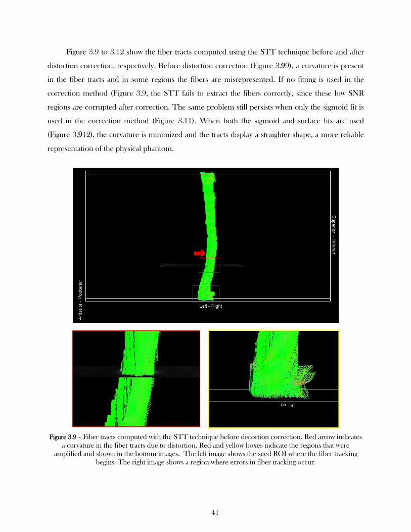
41
Figure 3.9 to 3.12 show the fiber tracts computed using the STT technique before and after
distortion correction, respectively. Before distortion correction (Figure 3.99), a curvature is present
in the fiber tracts and in some regions the fibers are misrepresented. If no fitting is used in the
correction method (Figure 3.9, the STT fails to extract the fibers correctly, since these low SNR
regions are corrupted after correction. The same problem still persists when only the sigmoid fit is
used in the correction method (Figure 3.11). When both the sigmoid and surface fits are used
(Figure 3.912), the curvature is minimized and the tracts display a straighter shape, a more reliable
representation of the physical phantom.
Figure 3.9 – Fiber tracts computed with the STT technique before distortion correction. Red arrow indicates
a curvature in the fiber tracts due to distortion. Red and yellow boxes indicate the regions that were
amplified and shown in the bottom images. The left image shows the seed ROI where the fiber tracking
begins. The right image shows a region where errors in fiber tracking occur.

42
Figure 3.10 – Fiber tracts computed with the STT technique after the correction with the original method
(without sigmoid or surface fit). Red arrow indicates a curvature in the fiber tracts due to distortion. Red and
yellow boxes indicate the regions that were amplified and shown in the bottom images. The left image
shows the seed ROI where the fiber tracking begins. The right image shows a region where errors in fiber
tracking occurs.
43
Figure 3.11 – Fiber tracts computed with the STT technique after distortion correction using only the
sigmoid fit. The curvature present in the figures is minimized. Red and yellow boxes indicate the regions that
were amplified and shown in the bottom images. The left image shows the seed ROI were the fiber tracking
begins. The right image shows a region were errors in fiber tracking occurred in the previous case.
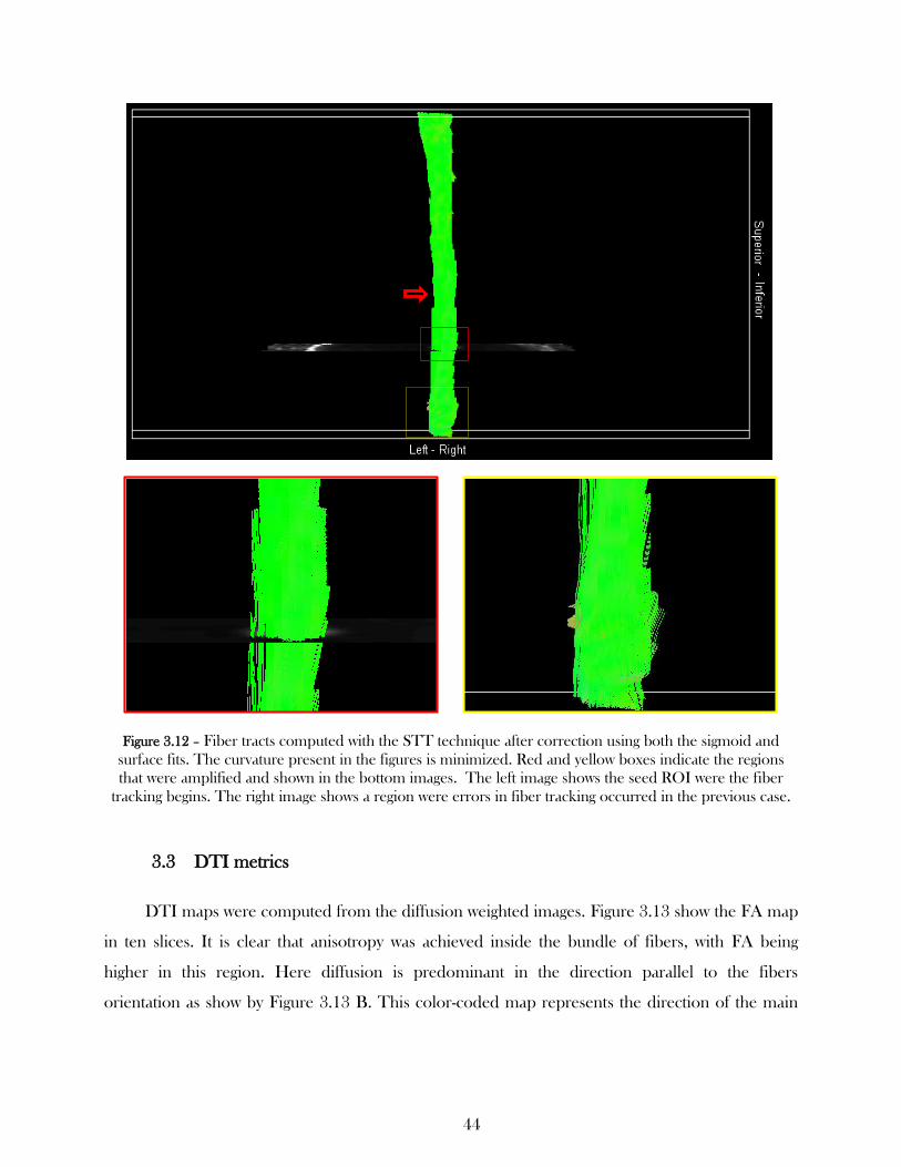
44
Figure 3.12 – Fiber tracts computed with the STT technique after correction using both the sigmoid and
surface fits. The curvature present in the figures is minimized. Red and yellow boxes indicate the regions
that were amplified and shown in the bottom images. The left image shows the seed ROI were the fiber
tracking begins. The right image shows a region were errors in fiber tracking occurred in the previous case.
3.3 DTI metrics
DTI maps were computed from the diffusion weighted images. Figure 3.13 show the FA map
in ten slices. It is clear that anisotropy was achieved inside the bundle of fibers, with FA being
higher in this region. Here diffusion is predominant in the direction parallel to the fibers
orientation as show by Figure 3.13 B. This color-coded map represents the direction of the main

45
eigenvector weighted by the value of FA. The fiber bundle has a red color, indicating that water
molecules are moving preferentially in the up-down direction.
Figure 3.13 – A: Color coded FA map. The colors are defined by the direction of the main eigenvector and
the amplitude is weighted by FA. Note the color code given by the arrow system. Diffusion in the up-down
direction is represented in red; Left-right is represented in green, and finally inwards-outwards of the plane is
represented by blue. B: FA maps of ten slices. The fiber bundle show higher values. Note the ROI
placement (in red) for the measurement of FA and ADC. C: ADC maps. Regions containing free water have
higher values. D: FA and ADC values in the fiber bundle over a period of 4 months. The Mann-Wallis test
shows no significant difference over time; p-value > 0.6.
Figure 3.13 C represents ADC maps. As expected, ADC is higher in the water surrounding
the fiber bundle. Nevertheless, in this region, ADC has the same order of magnitude.
In order to verify the stability and reproducibility of the phantom, ADC and FA were
measured several times over a period of 4 months and the result is shown in Figure 3.13 D.
0
0,2
0,4
1 2 3 4 5
FA
0,00E+004,00E-048,00E-041,20E-031,60E-032,00E-03
1 2 3 4 5MD
(m
m2
/s)
Scan number
A B
C D

46
Regions of interest were placed in the fiber bundles and FA and MD values were calculated. A
mean FA of 0.38 ± 0.20 and a mean MD of (1.50 ±0.04) x 10-3
mm2
/s were obtained. The Kruskal-
Wallis test shows no significant difference in these metrics over time (p-value > 0.6).
3.4 Healthy volunteer studies
Figure 3.14 shows images from healthy volunteers before distortion correction. The two EPI
images present distortions in opposite directions along the PE axis. These distortions are reflected
as sheering and compression of the structures, small undulations along the spine as well as
accentuated curvatures that are better displayed when the contour of the EPI images are
superimposed to the T2 FRFSE image. Apart from distortion there is also the presence of ghost
artifacts.
Figure 3.14 – Images from healthy volunteers before correction. Top: A: Dataset with left-right phase
encoding direction (blue arrow); B: Dataset with right-left phase encoding direction (blue arrow), the + and
– symbolically indicate the PE direction; C: Distortion-free T2 FRFSE image. Bottom: A: Contour (in
magenta) of the DTI-EPI + image superimposed to the T2 FRFSE; B: Contour of the DTI-EPI– image
superimposed to the T2 FRFSE; C: Contour of the T2 FRFSE superimposed to the respective image. Red
arrows indicate distortions. Yellow arrows indicate ghost artifact.
A B C
DTI-EPI + DTI-EPI -

47
Figure 3.15 shows the same images after correction. None of the methods is able to
completely correct the distortions. The three methods are able to correct the distortions in the
upper region of the image where ghost artifacts are minimal. However, in the lower regions were
ghosting is more severe, the correction is not efficient.
Figure 3.15 – Images from healthy volunteers after correction. Top A: Post correction using the original
method with no fitting; B: Result after distortion correction using only the sigmoid fit; C: Result after using
both the sigmoid and surface fit in the correction method. Bottom: Contour of the images on the top
superimposed to the distortion free T2 FRFSE images. Red arrows indicate regions where the correction
fails.
A B C
No fit Sigmoid Sigmoid+Surface

48
4 DISCUSSION
In this work, the first step was to determine the optimal coil configurations for the HNS coil
for imaging a structure such as the spinal cord, and also explore the possibilities of using parallel
imaging. This was performed with a coil decoupling experiment.
Previous studies [55] show that in a multi-channel or multi-element coil array there can be
noise induction or interference of one channel over the other. This can affect the information
gathered by each channel. This is relevant when we are interest in applying parallel imaging. With
this technique, the information collected by each channel is treated as independent of one another
and then combined to produce a final image. The influence of one channel over the other can also
be verified by studying the noise correlation matrix between the cannels.
This is also relevant in order to determine which coil configuration should be used to image
different regions of the spinal cord with this HNS coil. The coil has a total of 29 elements
connected to 16 channels and organized in 8 segments (the chest, face, and other 6 segments in the
posterior part).
In the upper section of the coil there is the possibility to use the face and chest part in
addition to segments 1-2, in order to have a greater coverage of the object of interest. Indeed it was
possible to verify that in the channels that were acquiring signal, higher SNR is achieved when using
the face and chest parts with groups 1-2 in contrast with the case where they are not used. In order
to successfully use parallel imaging, it would be ideal to have coil elements symmetrically
distributed over the imaged object. In spinal cord imaging, it is most common to use the anterior-
posterior direction as the PE direction since no aliasing of the shoulders and other structures would
occur over the spine. With this coil, the distribution of elements in the PE direction is relatively
symmetrical in the upper region where there are elements in the anterior and the posterior part of
the spine. This means that parallel imaging is possible in the upper section of the spine covered by
groups 1-2-3, the face and chest parts. Therefore it is advantageous to use the chest and face parts,
not only because of the increase of SNR but also due to the fact that it allows parallel imaging for
acceleration in the PE direction. In the lower regions, covered only by 4-5-6, parallel imaging
would only be possible if the PE direction was cranial-caudal. However, this is difficult to
accomplish because the phase FOV cannot cover the entire extent of the spinal cord which means
that the regions outside of the FOV would suffer aliasing.

49
Knowing that the SNR is higher when using the face and chest parts, the next step was to
keep these parts connected and add other elements in the posterior section (groups 3-4). As
additional elements are used, the SNR in the channels decreases. This may happen because the
decoupling circuit between the elements of the coil is not perfect, hence the channels are not totally
independent. For example, channels 1 to 7 are only acquiring signal from elements grouped in
groups 1-2, chest and face. The signals from elements grouped in groups 3-4-5-6 are acquired by
other channels. However, when these elements are connected, their noise also contributes to the
decrease in SNR in channels 1 to 7 that do not correspond to them. Thus when imaging specific
sections of the spinal cord, for instance the cervical spine, it is preferable to use the minimal
number of coil elements. In this case, one should only use groups 1-2, face and chest. The same
principle applies to the other sections of the spine. If bigger FOVs are intended when imaging
larger portions of the spine, this can be achieved by using more elements at the same time, with a
cost in SNR.
The next step in this work was the improvement of distortions in DTI images caused by
static field inhomogeneities. The algorithm used is based on a method that estimates the pixel
displacement map from two DTI-EPI images with opposite PE directions. The correct estimation
of the DM depends on several factors, including the SNR, the presence of other artifacts apart from
distortion (e.g. ghost, motion). One of the assumptions is that the two images, if not affected by
other artifacts, differ only in terms of distortions that will have opposite directions. Therefore, their
respective CDFs should have similar curves. This is ensured by fitting both CDFs to a sigmoid
function before calculating the DM. Moreover, the influence of SNR is minimized by removing
regions of low SNR form the DM. The new values of displacement in these regions are obtained
from a fitted polynomial surface. Indeed if no surface fit is used, the correction fails in regions of
low signal intensity (fiber bundle) due to erroneous estimation of pixel displacement.
In general, the distortions are more severe in the edges of the bottle. The small undulations
of the bottle are distorted and unrecognizable from the physical phantom. In fact, in these regions
the correction results are slightly better when no fitting is used. This occurs because there is always
a loss of information when the original CDF curves and DM are fitted to the sigmoid function and
polynomial surface, respectively. Visually, the uncorrected image presents low resemblance with the
T2 FRFSE image and this is confirmed by the MI. Statistical analysis shows an increase of MI
between the distortion free T2 FRFSE and DTI-EPI images when the correction is applied.
However, no significant difference was found between the methods (the original reversed gradient
50
method with no fitting, with the sigmoid fit and with the surface fit). This is due to the fact that the
calculation of MI is based on the entire image. Therefore, the regions where the correction
methods differ (low SNR regions) are too small to make a significant difference on the value of MI.
Nevertheless, by visual inspection it is clear that using the sigmoid and the surface fit is
advantageous for the improvement of the image quality (Figure 3.7). This is emphasized after the
estimation of the fiber tracts (Figures 3.9 – 3.12). The fiber bundle is not accurately represented in
the uncorrected image or when no fitting is used in the correction method. When only the sigmoid
fit is used, the estimation of the fiber tracts is also corrupted because the fiber bundles have low
SNR in the DTI images. As mentioned before, the sigmoid fit alone is not sufficient for a correct
estimation of the DM in low SNR regions. Only when both the sigmoid and surface fits are used,
do the fiber tracts have a more reliable shape and resemblance with the physical fiber bundle.
In order to study the reproducibility and stability of the phantom, FA and ADC maps were
calculated over time and their values were measured in ROIs placed in the fiber bundle. The
results show that an anisotropic diffusion was achieved inside the fiber bundles, with water diffusing
predominantly in the direction parallel to the fibers as expected. The ADC value is within the
expected range and the FA value was slightly lower than observed in white matter of the spinal cord
(FA between 0.4 and 0.75) [31, 32, 34]. This may be explained by the fact that the phantom is only
a simplification of reality. Here, the anisotropic diffusion is only created by the molecules between
the fibers (extracellular space). Moreover, diffusion is also dependent on the composition of the
fluid and its temperature, which are not the same as in the spinal cord. Nonetheless, the phantom
was stable over time and FA and ADC did not display significant variations.
Lastly, the distortion correction method was applied to human data. Images from the
brainstem and the cervical spinal cord were obtained. When compared to the T2 FRFSE, the DTI
images present distortions mainly along the phase encoding direction. Here, the curvature of the
spine is misrepresented. Furthermore, there are ghost artifacts that influence the correction. The
method works in regions where ghost artifacts are minimal, but fails in regions where they are more
severe. This happens because these artifacts are not the same for the two EPI images. There is no
linearity for the ghost artifacts between the two images. For example, in an inverse line of thought,
with the DM and the EPI+ image, one can estimate the EPI- image. However, if the EPI+ image
has ghosts, it is not possible to correctly estimate the second image. Therefore, when the DM map
is estimated from the two EPI images, the pixel displacement values obtained are corrupted
because errors occur during the estimation of the CFD.

51
5 CONCLUSION AND PERSPECTIVES
DTI is gaining relevance in clinical studies including the spinal cord. However, imaging this
organ is not straight-forward and many challenges may arise. In longitudinal MR studies with the
spinal cord, test-objects are always relevant for the optimization of protocols and methods for the
improvement of image quality.
The phantom presented in this work is a simplification of the complex structure of the spinal
cord but it was easily constructed with cheap materials and during the course of the study it was a
reliable and reproducible object that allowed a continuous optimization of the DTI protocol, coil
configurations and improvement of distortion correction method. Moreover, the novelties
proposed for the correction method, namely the sigmoid and surface fit, proved to be robust
improvement of distortions both in regions of low SNR and regions of higher SNR.
Future work will reside on the improvement of the phantom, with more complex structures
(curved shapes and crossing fibers,) that are more accurate representations of the spinal cord.
Different fiber dimension and materials can also be explored. As for the correction method, when
transposed to human data, other challenges apart from susceptibly distortions, such as ghost
artifacts, must also be taken in account in order to improve the robustness of the correction
method.

52
REFERENCES
[1] J. E. T. E. O. Stejskal, “Spin Diffusion Measurements: Spin Echos in the Presence of a
Time Dependent Field Gradient,” JCP, vol. 42, no. 1, pp. 288–292, 1965.
[2] “MRI online course (Magnetic Resonance Imaging),” IMAIOS. [Online]. Available:
https://www.imaios.com/en/e-Courses/e-MRI. [Accessed: 07-Dec-2015].
[3] E. M. Haacke, R. W. Brown, M. R. Thompson, and R. Venkatesan, Magnetic Resonance
Imaging: Physical Principles and Sequence Design. Wiley, 1999.
[4] H. Y. Carr and E. M. Purcell, “Effects of Diffusion on Free Precession in Nuclear Magnetic
Resonance Experiments,” Phys. Rev., vol. 94, no. 3, pp. 630–638, May 1954.
[5] W. S. Price, “Pulsed-field gradient nuclear magnetic resonance as a tool for studying
translational diffusion: Part 1. Basic theory,” Concepts Magn. Reson., vol. 9, no. 5, pp. 299–
336, Jan. 1997.
[6] T. Schneider, “Spinal cord diffusion imaging: Challenging characterization and prognostic
value,” Doctoral Thesis, UCL (University College London), 2013.
[7] Bammer, F. Fazekas, M. Augustin, J. Simbrunner, S. Strasser-Fuchs, T. Seifert, R.
Stollberger, and H. P. Hartung, “Diffusion-weighted MR imaging of the spinal cord,” AJNR Am J Neuroradiol, vol. 21, no. 3, pp. 587–591, Mar. 2000.
[8] P. J. Basser, J. Mattiello, and D. LeBihan, “Estimation of the effective self-diffusion tensor
from the NMR spin echo,” J Magn Reson B, vol. 103, no. 3, pp. 247–254, Mar. 1994.
[9] P. J. Basser and C. Pierpaoli, “Microstructural and physiological features of tissues
elucidated by quantitative-diffusion-tensor MRI,” J Magn Reson B, vol. 111, no. 3, pp. 209–
219, Jun. 1996.
[10] P. B. Kingsley, “Introduction to diffusion tensor imaging mathematics: Part III. Tensor
calculation, noise, simulations, and optimization,” Concepts Magn. Reson., vol. 28A, no. 2,
pp. 155–179, Mar. 2006.
[11] A. Kumar, D. Welti, and R. R. Ernst, “NMR Fourier zeugmatography. 1975,” J. Magn. Reson., vol. 213, no. 2, pp. 495–509, Dec. 2011.
[12] M. Poustchi-Amin, S. A. Mirowitz, J. J. Brown, R. C. McKinstry, and T. Li, “Principles and
applications of echo-planar imaging: a review for the general radiologist,” Radiographics,
vol. 21, no. 3, pp. 767–779, Jun. 2001.

53
[13] A. Deshmane, V. Gulani, M. A. Griswold, and N. Seiberlich, “Parallel MR imaging,” J Magn Reson Imaging, vol. 36, no. 1, pp. 55–72, Jul. 2012.
[14] R. Brown, Y.-C Cheng, E. Haacke, M. Thompson, e R. Venkatesan, «Sampling and
Aliasing in Image Reconstruction», in Magnetic Resonance Imaging, John Wiley & Sons
Ltd, 2014, pp. 669–700.
[15] K. P. Pruessmann, M. Weiger, M. B. Scheidegger, and P. Boesiger, “SENSE: sensitivity
encoding for fast MRI,” Magn Reson Med, vol. 42, no. 5, pp. 952–962, Nov. 1999.
[16] M. A. Griswold, P. M. Jakob, R. M. Heidemann, M. Nittka, V. Jellus, J. Wang, B. Kiefer,
and A. Haase, “Generalized autocalibrating partially parallel acquisitions (GRAPPA),”
Magn Reson Med, vol. 47, no. 6, pp. 1202–1210, Jun. 2002.
[17] J. Puly, Chapter 2: Partial Fourier Reconstruction, Lecture Notes http://users.fmrib.ox.ac.uk/~karla/reading_group/lecture_notes/Recon_Pauly_read.pdf, Standford University, [Available online February 2016].
[18] X. Liu, “Magnetic Resonance Diffusion Tensor Imaging: Distortion Correction Methods
and Their Applications in High-Resolution In vivo Monkey Brain Scans,” Doctoral Thesis,
University of Rochester, Rochester, New York, 2009.
[19] P. Jezzard e R. S. Balaban, «Correction for geometric distortion in echo planar images from
B0 field variations», Magn Reson Med, vol. 34, n. 1, pp. 65–73, Jul. 1995.
[20] H. Zeng e R. T. Constable, «Image distortion correction in EPI: Comparison of field
mapping with point spread function mapping», Magn. Reson. Med., vol. 48, n. 1, pp. 137–
146, Jul. 2002.
[21] Chang H, Fitzpatrick JM. A technique for accurate magnetic resonance imaging in the
presence of field inhomogeneities. IEEE Trans Med Imaging 1992;11:319–29.
[22] H. U. Voss, R. Watts, A. M. Uluğ, e D. Ballon, «Fiber tracking in the cervical spine and
inferior brain regions with reversed gradient diffusion tensor imaging», Magn Reson Imaging, vol. 24, n. 3, pp. 231–239, Abr. 2006.
[23] D. Weishaupt, V. D. Köchli, and B. Marincek, How does MRI work?: An Introduction to the Physics and Function of Magnetic Resonance Imaging. Springer Science & Business
Media, 2008.
[24] E. U. Saritas, S. J. Holdsworth, and R. Bammer, “Chapter 2.3 - Susceptibility Artifacts,” in
Quantitative MRI of the Spinal Cord, J. C.-A. A. M. Wheeler-Kingshott, Ed. San Diego:
Academic Press, 2014, pp. 91–105.
[25] J. B. Andre and R. Bammer, “Advanced Diffusion-Weighted Magnetic Resonance Imaging
Techniques of the Human Spinal Cord,” Top Magn Reson Imaging, vol. 21, no. 6, pp.
367–378, Dec. 2010.

54
[26] A. W. Anderson and J. C. Gore, “Analysis and correction of motion artifacts in diffusion
weighted imaging,” Magn Reson Med, vol. 32, no. 3, pp. 379–387, Sep. 1994.
[27] G. Zaharchuk, E. U. Saritas, J. B. Andre, C. T. Chin, J. Rosenberg, T. J. Brosnan, A.
Shankaranarayan, D. G. Nishimura, and N. J. Fischbein, “Reduced field-of-view diffusion
imaging of the human spinal cord: comparison with conventional single-shot echo-planar
imaging,” AJNR Am J Neuroradiol, vol. 32, no. 5, pp. 813–820, May 2011.
[28] E. U. Saritas, C. H. Cunningham, J. H. Lee, E. T. Han, and D. G. Nishimura, “DWI of
the spinal cord with reduced FOV single-shot EPI,” Magn Reson Med, vol. 60, no. 2, pp.
468–473, Aug. 2008.
[29]. C. Beaulieu, “The basis of anisotropic water diffusion in the nervous system - a technical
review,” NMR Biomed, vol. 15, no. 7–8, pp. 435–455, Dec. 2002.
[30] M. E. Moseley, Y. Cohen, J. Kucharczyk, J. Mintorovitch, H. S. Asgari, M. F. Wendland,
J. Tsuruda, and D. Norman, “Diffusion-weighted MR imaging of anisotropic water diffusion
in cat central nervous system,” Radiology, vol. 176, no. 2, pp. 439–445, Aug. 1990.
[31] B. M. Ellingson, S. N. Kurpad, S.-J. Li, and B. D. Schmit, “In vivo diffusion tensor imaging
of the rat spinal cord at 9.4T,” J Magn Reson Imaging, vol. 27, no. 3, pp. 634–642, Mar.
2008.
[32] J. C. Ford, D. B. Hackney, D. C. Alsop, H. Jara, P. M. Joseph, C. M. Hand, and P. Black,
“MRI characterization of diffusion coefficients in a rat spinal cord injury model,” Magn
Reson Med, vol. 31, no. 5, pp. 488–494, May 1994.
[33] B. M. Ellingson, S. N. Kurpad, and B. D. Schmit, “Ex vivo diffusion tensor imaging and
quantitative tractography of the rat spinal cord during long-term recovery from moderate
spinal contusion,” J Magn Reson Imaging, vol. 28, no. 5, pp. 1068–1079, Nov. 2008.
[34] C. A. Clark, G. J. Barker, and P. S. Tofts, “Magnetic resonance diffusion imaging of the
human cervical spinal cord in vivo,” Magn Reson Med, vol. 41, no. 6, pp. 1269–1273, Jun.
1999.
[35] M. Ries, R. A. Jones, V. Dousset, and C. T. Moonen, “Diffusion tensor MRI of the spinal
cord,” Magn Reson Med, vol. 44, no. 6, pp. 884–892, Dec. 2000.
[36] M. Descoteaux and J. G. Webster, “High Angular Resolution Diffusion Imaging
(HARDI),” in Wiley Encyclopedia of Electrical and Electronics Engineering, John Wiley &
Sons, Inc., 1999.
[37] D. S. Tuch, “Q-ball imaging,” Magn Reson Med, vol. 52, no. 6, pp. 1358–1372, Dec. 2004.

55
[38] J. Cohen-Adad, M. Descoteaux, S. Rossignol, R. D. Hoge, R. Deriche, and H. Benali,
“Detection of multiple pathways in the spinal cord using q-ball imaging,” Neuroimage, vol.
42, no. 2, pp. 739–749, Aug. 2008.
[39] B. M. Ellingson, J. L. Ulmer, S. N. Kurpad, and B. D. Schmit, “Diffusion tensor MR
imaging of the neurologically intact human spinal cord,” AJNR Am J Neuroradiol, vol. 29,
no. 7, pp. 1279–1284, Aug. 2008.
[40] D. Facon, A. Ozanne, P. Fillard, J.-F. Lepeintre, C. Tournoux-Facon, and D. Ducreux,
“MR diffusion tensor imaging and fiber tracking in spinal cord compression,” AJNR Am J
Neuroradiol, vol. 26, no. 6, pp. 1587–1594, Jul. 2005.
[41] S. Rajasekaran, R. M. Kanna, R. Karunanithi, and A. P. Shetty, “Diffusion tensor
tractography demonstration of partially injured spinal cord tracts in a patient with
posttraumatic Brown Sequard syndrome,” J Magn Reson Imaging, vol. 32, no. 4, pp. 978–
981, Oct. 2010.
[42] D. Ducreux, J.-F. Lepeintre, P. Fillard, C. Loureiro, M. Tadié, and P. Lasjaunias, “MR
diffusion tensor imaging and fiber tracking in 5 spinal cord astrocytomas,” AJNR Am J Neuroradiol, vol. 27, no. 1, pp. 214–216, Jan. 2006.
[43] D. M. Wingerchuk, C. F. Lucchinetti, and J. H. Noseworthy, “Multiple Sclerosis: Current
Pathophysiological Concepts,” Lab Invest, vol. 81, no. 3, pp. 263–281, Jan. 2001.
[44] E. Sbardella, F. Tona, N. Petsas, P. Pantano, E. Sbardella, F. Tona, N. Petsas, and P.
Pantano, “DTI Measurements in Multiple Sclerosis: Evaluation of Brain Damage and
Clinical Implications, DTI Measurements in Multiple Sclerosis: Evaluation of Brain
Damage and Clinical Implications,” Multiple Sclerosis International, Multiple Sclerosis International, vol. 2013, 2013, p. e671730, Mar. 2013.
[45] F. Fink, J. Klein, M. Lanz, T. Mitrovics, M. Lentschig, H. K. Hahn, and H. Hildebrandt,
“Comparison of Diffusion Tensor-Based Tractography and Quantified Brain Atrophy for
Analyzing Demyelination and Axonal Loss in MS,” Journal of Neuroimaging, vol. 20, no. 4,
pp. 334–344, Oct. 2010.
[46] R. Brown, Y.-C Cheng, E. Haacke, M. Thompson, e R. Venkatesan, «Sampling and
Aliasing in Image Reconstruction», in Magnetic Resonance Imaging, John Wiley & Sons
Ltd, 2014, pp. 669–700.
[47] P. Li, X. Yu, J. Griffin, J. M. Levine, e J. Ji, «High-resolution MRI of spinal cords by
compressive sensing parallel imaging», em 2015 37th Annual International Conference of the IEEE Engineering in Medicine and Biology Society (EMBC), 2015, pp. 4266–4269.
[48] Questions and Answers in MRI, http://mriquestions.com/array-coils.html [Available
Online September 2016].
[49] R. F. Lee, R. O. Giaquinto, e C. J. Hardy, «Coupling and decoupling theory and its

56
application to the MRI phased array», Magn Reson Med, vol. 48, n. 1, pp. 203–213, Jul.
2002.
[50] R. F. Lee, R. O. Giaquinto, e C. J. Hardy, «Coupling and decoupling theory and its
application to the MRI phased array», Magn Reson Med, vol. 48, n. 1, pp. 203–213, Jul.
2002.
[51] M. A. Bernstein, K. F. King, e X. J. Zhou, Handbook of MRI Pulse Sequences. Elsevier,
2004.
[52] D. B. Russakoff, C. Tomasi, T. Rohlfing, e C. R. M. Jr, «Image Similarity Using Mutual
Information of Regions», in Computer Vision - ECCV 2004, T. Pajdla e J. Matas, Eds.
Springer Berlin Heidelberg, 2004, pp. 596–607.
[53] A. Collignon, F. Maes, D. Delaere, D. Vandermeulen, P. Suetens, e G. Marchal,
«Automated multi-modality image registration based on information theory», In: Bizais, 1995.
[54] Chang Chia-Hao, “DtiSearch - DTI Fiber Tractography (Streamline Tracking Technique)”,
NTHU Magnetic Resonance Imaging Laboratory Department of Biomedical Engineering
and Environmental Sciences, 2012 [Available online January 2016].
https://www.mathworks.com/matlabcentral/fileexchange/34008-dti-fiber-tractography--
streamline-tracking-technique-/all_files.
[55] A. Sewonu, “DéveloppementsMéthodologiques et Techniques pour le Contrôle Qualité en
Imagerie par RésonanceMagnétique”, École Doctorale BioSE (Biologie-Santé-
Environnement), Doctoral Thesis, Université de Lorraine, 2014. [Available Online
September 2016] http://docnum.univ-
lorraine.fr/public/DDOC_T_2014_0002_SEWONU.pdf
[56] M. Bai e S. Luo, «Improved Fiber Tracking for Diffusion Tensor MRI», em Medical Imaging and Augmented Reality, G.-Z. Yang e T.-Z. Jiang, Eds. Springer Berlin Heidelberg,
2004, pp. 171–178.
[57] Inglese M, Bester M. “Diffusion imaging in multiple sclerosis: research and clinical
implications”. NMR in biomedicine. 2010;23(7):865-872. doi:10.1002/nbm.1515.

57
APPENDIX I
TEDI - Tool for EPI Distortion Improvement
Requirements:
This interface was created using Matlab R2013a (version 8.1) under Linux environment. It
is recommended using this or later versions of Matlab. In order to successfully use this interface
connection between Matlab and Archimed3 (database for the images) is necessary. Moreover some
inhouse Matlab functions in the database are called. Before starting the interface set the path to
these functions. <Add to path> <Select folders and subfolders>. Everything (including the files to
run the interface tedicor.fig and tedicor.m) are in the zipped folder “workspace”:
Summary:
TEDI is a Matlab interface for the correction of EPI distortions in DTI images. The
correction methods are based on the reversed gradient method describe in this thesis. For this
method to work, two EPI images with opposite phase encoding direction must have been acquired.
Theoretically, these two images will have distortions in opposite direction in the PE direction and
can be combined to produce the undistorted image. A detailed description of the interface is given
in this tutorial. The order of execution of each panel is as follows 1. Import Data from Archimed,
2. Correction, 3. Corrected, 4. Stats.
A figure of the full interface is displayed bellow.

58
1. Import Images from Archimed
To start double click on the tedicor.fig file or open the tedicor.m in Matlab and run the
code;
First, specify the exam code and the series of the two DTI datasets and the T2FRFSE
dataset (without distortions) for comparison. The images are imported as 3D volumes in
“signed 16-bit” format (int16). For the DTI images, the size is (Nx, Ny, Nz), where Nx and
Ny are the dimension of the image in pixels and Nz is the number of slices times the
number of diffusion directions (including the b0 measurement). For the FRFSE image Nz is
the number of slices;
Then press the Load button to import the images;
A window will pop up to specify the slice orientation for this dataset;

59
In the left panel, the first DTI dataset is automatically displayed;
In the right panel toggle between the FRFSE and the second DTI dataset;
Change contrast and intensity using the sliders to better visualize the images;
Scroll between different slices (and diffusion directions in the case of the DTI datasets);
2. Reversed Gradient Correction
Choose the fit options for the calculation of the displacement map for the correction. For
more details about each fit option (Original, Surface Fit, Sigmoid Fit, Sigmoid + Surface Fit)
read section 2.4.3 of this thesis;
Choose the number of iterations (1, 2, 3) and registration options (None, Rigid, Affine); 1
Iteration and no registration are recommended.
Press on the bear logo button to apply correction;
Toggle between the two images

60
3. Corrected
This panel displays the results after the correction;
Toggle between the Corrected, Uncorrected, FRFSE images and the pixel Displacement
map;
Change contrast and intensity using the sliders to better visualize the images;
Scroll between different slices (and diffusion directions in the case of the DTI dataset);
Apply correction
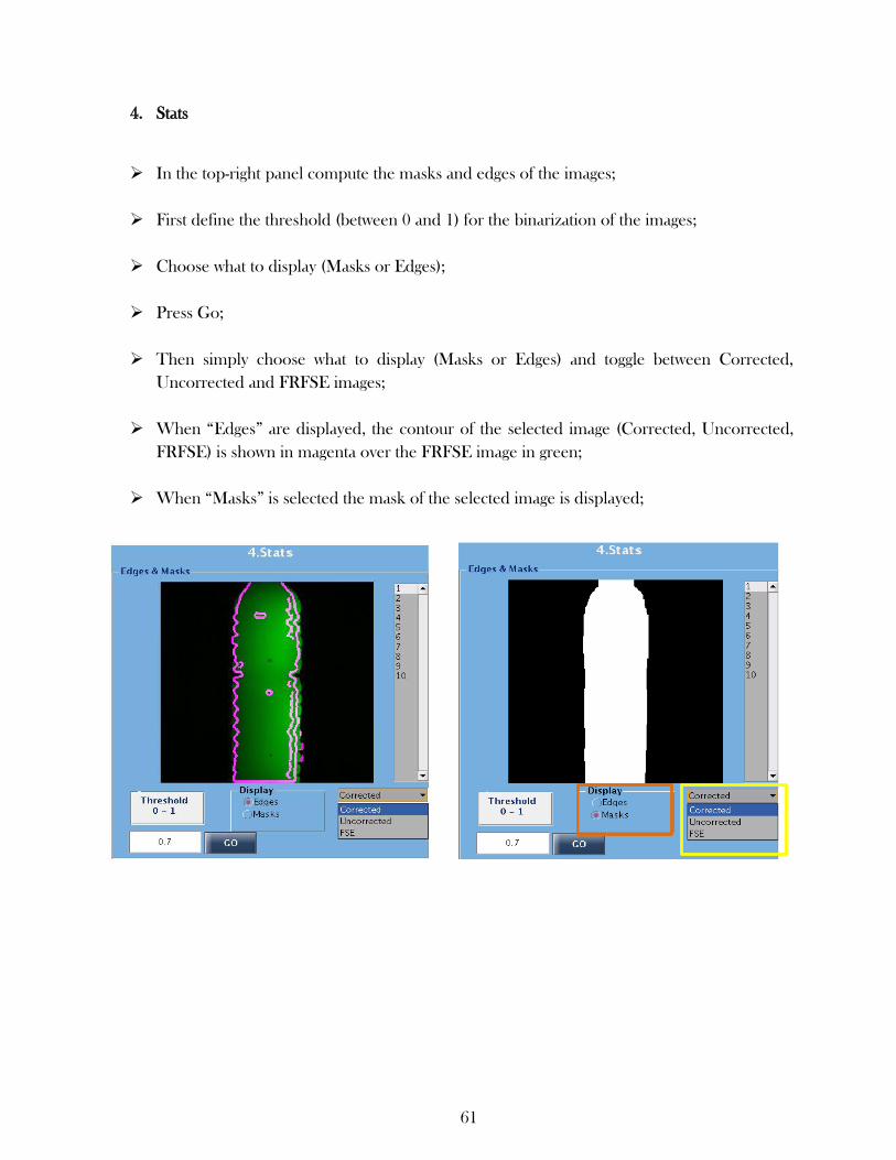
61
4. Stats
In the top-right panel compute the masks and edges of the images;
First define the threshold (between 0 and 1) for the binarization of the images;
Choose what to display (Masks or Edges);
Press Go;
Then simply choose what to display (Masks or Edges) and toggle between Corrected,
Uncorrected and FRFSE images;
When “Edges” are displayed, the contour of the selected image (Corrected, Uncorrected,
FRFSE) is shown in magenta over the FRFSE image in green;
When “Masks” is selected the mask of the selected image is displayed;

62
In the bottom-right panel compute the mutual information. In this case the MI is being
calculated between the uncorrected image and the distortion-free FRFSE image and
between the corrected image and the distortion-free FRFSE image;
Choose if the MI is computed in the “Whole Image” or in the “Masked image”;
Press Go;
Boxplots are displayed. The values are from all the slice;
Progress and Report
Here, error messages and the computation progress are displayed.
The mean values of the mutual information computed above are also displayed here;

63
Press Clear to clean the message board;
Press Save to save the data in a .mat file; specify a name (e.g. “data”) and a path;
Press Exit to exit the program;
After the data is saved it can be loaded it into Matlab workspace;
The data is saved as a structure and some relevant fields are displayed in the figure below.
Top Related