


Languages
Pages
Legal


Design of a Data Analysis System for Walking Robots.
A Design Project Report
Presented to the Engineering Division of the Graduate School
of Cornell University
in Partial Fulfillment of the Requirements for the Degree of
Masters of Engineering
by
Leticia Rojas Camargo
Project Advisor: Andy Ruina
Degree Date: January 2009

Abstract
Masters of Engineering in Mechanical and Aerospace engineeing
Cornell University
Design Project Report
Project title:
Design of a Data Analysis System for Walking Robots.
Author:
Leticia Rojas Camargo
Abstract:
The main goal of this project was to design a tool to simplify the data visualization and data analysis for our robotics research. At the end of the project the goal is to have a functional data analysis program that incorporates our specific visualization and analysis needs, as well as the option of visualizing and analyzing data alongside a video. MATLAB was chosen as a platform for programming the data analysis tool. The final program consists of a data analysis and a data with video analysis option. The functions that the program is capable of doing are divided in three sections, the data visualization functions, the data analysis function and the video functions. The data visualization functions are changing the data file to analyze, changing the variables plotted, moving the cursor to an exact time point, moving discretely along data points, choosing the min and max values of time to be plotted, changing the min and max values of the variables to be plotted, zooming in and out in time and in the variables and showing error messages. The data analysis functions are plotting two variables against each other, plotting more than one variable against time on the same graph, scaling a variable and entering a MATLAB function into the data. The video analysis tools are moving frame by frame and playing and stopping the video in synch with the data and synchronizing the video and data to a new synch point.
Report Approved By:
Project Advisor: Andy Ruina
Signature: ______________________________ Date:_____________

Table of contents
Table of contents i
Index of figures iii
1. Introduction 1
1.1 Motivation 1
1.2 The MATLAB based GUI 2
1.3 Report structure 3
2. Problem Statement 5
2.1 Problem statemen 5
2.2 Design objectives 6
2.3 Requirements 6
3. The data analysis GUI 8
3.1 Program structure 8
3.2 The data analysis GUI 9
3.2.1 Data Only GUI 10
3.2.2 The Data and Video GUI 12
3.3 Functions 14
4. Data display 16
4.1 Data file reading 16
4.2 Plot display 18
4.3 Zoom functions 20
4.4 Error display 22
5. Data analysis 24
5.1 Scaling a variable 24
i

5.2 Plotting two variables against each other 26
5.3 Plotting several variables in one graph 27
5.4 Manipulating a variable 29
6. Combined video and data analysis 31
6.1 Video reading. 31
6.2 The video display window 32
6.2.1 Video functions 33
6.3 Data and video synchronization 34
6.4 Video capturing and deinterlacing 35
6.5 Limitations 37
7. Conclusions 39
8. References 40
A.1 Source Code for the Data Analysis program 41
ii

Index of figures and tables
Figure 1.1. The data analysis MATLAB GUI. 3
Figure 3.1. Initial Prompt 10
Figure 3.2. Data file open prompt. 10
Figure 3.3 The MATLAB data analysis GUI (Data display only). 11
Figure 3.4. Help Menu 12
Figure 3.5. Video file open prompt 13
Figure 3.6. The MATLAB data analysis GUI (Data and video display). 14
Figure 4.1. Sample data file 17
Figure 4.2 Error message if data file is not chosen 18
Figure 4.3. Plot display 18
Figure 4.4. Variable list 19
Figure 4.5. Variable change prompt 20
Figure 4.6. Moving cursor to a user chosen time. 20
Figure 4.7. Changing maximum and minimum values of t. 21
Figure 4.8. Changing max. and min. values of a variable. 22
Figure 4.9. Error Display 23
Figure 5.1. Scaling a Variable 25
Figure 5.2. Loadcell variable, a)before scaling, b) after scaling 26
Figure 5.3. Plotting two variables against each other 26
Figure 5.4. PWM vs Torque plot 27
Figure 5.5. Plotting several variables on the same graph 28
Figure 5.6. Angle comparison plot 28
iii

iv
Figure 5.7. Manipulating the data. 29
Figure 5.8. Manipulated data plot 30
Figure 6.1. The video display window 33
Figure 6.2. Button functions 34
Figure 6.3. Video to data toggle message 34
Figure 6.4. Synchronization success message 35
Figure 6.5. Data to video toggle message 35
Figure 6.6. Deinterlacing a video with VirtualDub 37
Table 3.1 Data display functions 14
Table 3.2 Data analysis functions 15
Table 3.3 Video and data analysis functions. 15

1. Introduction
1.1 Motivation
The need for a data analysis tool became more pressing as the Cornell Ranger team
prepared for a record breaking walk and problems with the robot arose. The main
motivation for this project was driven from that one basic need that had not been fulfilled
until now. This data analysis program would provide us with an easy to use data display to
visualize possible unexpected behavior or errors as soon as they happened, as well as more
advanced tools to analyze the data more thoroughly after a walk or test.
Having the ability to perform these tasks with ease would help us greatly to achieve the
goals the team had set. Thus, making a program that could incorporate both, and even
more incorporate the reading and analysis needs of the different team members working
with the robot, became a priority.
1

The less pressing but certainly important issue of including video reading with data
synchronization into the data analysis was also considered and integrated at a later stage of
the project.
1.2 The MATLAB based GUI
Up until now, all the data analysis of the robot had been done by directly reading the
robot’s data file and plotting the data needed in MATLAB, and having to repeat the
operation every time we needed to analyze certain data. This was often a time consuming
task that if simplified, would be of much help for the team.
Making a GUI (Graphical User Interface) for the data analysis was the best option for
creating a user friendly data analysis program. Since most of the data analysis was already
done with the help of MATLAB, and because MATLAB is a powerful tool for this
purpose, it was decided to take advantage of the GUI programming capabilities of
MATLAB.
2

Figure 1.1. The data analysis MATLAB GUI.
1.3 Report structure
This report is designed to serve as both a technical report of the data analysis gui as well as
the documentation of the software for users of the program and future developers in the
case that more features are needed.
The Design problem section will focus on familiarizing the reader with the goal and the
main requirements of the project, as well as the main challenges faced in programming the
tool.
3

The following section will explain the general structure of the data analysis GUI. It will
also serve as a user’s guide and provide a brief description of the functions available to the
user.
Next the report will proceed to the technical details and characteristics of the data analysis
functions, dividing them in three sections. The first of these sections will focus on the data
reading and display. It will explain the way the data is read from the data file. It will also
focus on the display functions of zooming, changing plots and showing errors.
The following section will focus on the data analysis functions of the program. Each of the
data analysis functions of scaling a variable, plotting two variables against each other,
plotting more than one variable on the same plot will be justified within the context of the
needs of our team. This section will also have a description of the implementation and use
of each of these functions.
The third and final section of this report will center on the combined video and data
analysis option of the program. In this section, the differences between the data only and
data and video GUI windows will be explained. The section will also cover the way the
video is read into MATLAB, as well as its playback and synchronization with the data
characteristics. Finally this section considers the limitations of the video reading
capabilities of MATLAB.
4

2. Problem statement
2.1 Problem Statement
Communication with the Cornell Ranger Robot is made through a wireless data acquisition
card. It sends and receives data through a LabView interface. LabView then generates a
data file from the received data from the robot sensors. Currently, up to 25 different
variables can be collected into the data file. The contents of the data file help to diagnose
problems with the robot, as well as understanding how it works and matching it with a
simulation of the system.
This Masters of Engineering project was born from the need of a general data analysis tool
for the robot. This tool should help all of those working on the robot to visualize and
analyze its data. The problem solving scheme can be divided into two stages. The first one
is developing a functional and user friendly data analysis GUI that incorporates the
5

different data analysis needs of the team. The second stage will be to include video
synchronization into the data analysis.
2.2 Design objectives
The main goals of this project are:
• To have a functional and easy to use data display and analysis tool for the Cornell
Ranger Robot.
• To incorporate into the program the necessary functions to meet the data analysis
needs of the Cornell Ranger Teams.
• To have the option of combined video and data analysis capabilities that are not
limited by the video format.
• To be able to easily upgrade the code to accommodate new analysis needs, both for
the Cornell Ranger Robot as well as future robots.
2.3 Requirements
The requirements of the MATLAB data analysis program were decided taking into account
the different needs of the team, while taking into account the format of the data we got from
the data acquisition.
6

The data display requirements of the GUI are:
• One of more plots should be able to be displayed at once.
• It should show the value of the plotted variable at a certain time chosen through a
cursor.
• It should allow the users to change which and how many plots they want to see.
• It should allow zooming in both in time (x axis) and variable (y axis).
• It should have is the capability to display errors.
The data analysis requirements are:
• It should be able to plot 2 variables against each other.
• It should be able to plot several variables on the same plot for comparison.
• It should have is a scaling function.
• It should allow the user to mathematically manipulate a variable.
For the video and data analysis the requirements are
• It should be able to read the videos captured with either of the lab cameras, as well
as to have the possibility of reading videos captured with other devices.
• The user should be able to synchronize the video with the data and play it-back
simultaneously.
• The user should be able to move through the video frame by frame and also fast-
forward and backwards.
• We should be able to get as much frames per second from our cameras as we can.
7

3. The data analysis GUI
The following section is intended to familiarize the reader with the data analysis program.
This section contains the structure of the program, a guide to the use of the GUI and a
description of all the functions available to the user,
3.1 Program structure
The data analysis program for the Cornell Ranger Robot is a MATLAB based GUI. It is
made of a startup file, two main program files and three function files. These files are:
• startdataanalysis.m: The startup file. Running this m-file will start the GUI and let
the user choose the option of reading a video file along with the data.
8

• graphs_dataanalysis.m: This is the data analysis only program file. If the user
chooses to analyze data without video, this file will be used. Its GUI consists of a
single window and different functions are called back using the keyboard.
• graphs_videoread.m: This is the data and video analysis program file. If the user
chooses the option to read data along with video, this is the file that will be used.
Its GUI consists of two windows, a video display window with buttons to control
the video options, and a data display window, identical to the no-video GUI window
except for the synchronization functions.
• initgraphs.m: First of two data reading functions. This function is used to prompt the
user to open a data file and returns the filename and path information.
• rdfile.m: Second of two data reading functions. This function takes the file name and
path information from initgraphs.m and opens the data file information.
• The mmread function folder: This is a third party function used to read video files
regardless of its format.
3.2 The data analysis GUI
Upon running startdataanalysis.m, the user will be prompted to decide if they want to work
with video and data or only data, as seen in fig. 3.1. The default option is No (Data Only)/
9

Figure 3.1. Initial Prompt
3.2.1 Data Only GUI.
If the user chooses to not read a video, the Data Only GUI will be launched. The first thing
it does is prompt the user to select a data file (fig. 3.2). This data file is obtained from the
data acquisition program for the robot and is in *.txt format.
Figure 3.2. Data file open prompt.
10

Once the user selects the data file, the program reads the data into MATLAB, and into the
GUI. The main window will then be launched (fig 3.2).
Figure 3.3 The MATLAB data analysis GUI (Data display only).
By default, the program plots the first four variables of the data file. These variables can be
changed by pressing the C key. The program displays the values of the variables at the
time denoted by the red cursor. This cursor can be moved using the LEFT and RIGHT
arrow keys or by pointing and clicking with the mouse at the desired position.
11

Pressing the H key will bring out the help menu (fig 3.4). This menu provides a quick
guide of the different functions available in the program and its corresponding callback
keys. To call a function the user must press okay to close the help menu, once in the main
window the user can proceed to press the corresponding callback key of the function.
Figure 3.4. Help Menu
3.2.2 The Data and Video GUI
If the option to read a video with the data is chosen in the initial prompt (fig 3.1), the Data
and Video GUI will be launched. Like in the Data Only version, a prompt to choose a data
file pops up (fig 3.2). However, once the data file is chosen a second file opening prompt
appears, allowing the user to choose a video file (fig 3.5)
12

Figure 3.5. Video file open prompt
After both the video and the data are read into the program, the video display and the data
display windows are loaded (fig 3.6). The data display window opens with same default
options of the data only version. Also by default the video display functions are on and the
data display options can’t be used. To use the data display options, press the Go to data
window button to toggle completely to the data display window or the Allow graph functions
button to use one function and return immediately to the video display. The user can
navigate through the video with the different buttons or the slider on the video display
window.
13

Figure 3.6. The MATLAB data analysis GUI (Data and video display).
3.3 Functions
In the following subsection we will show a brief overview of all the functions. The
functions are called back by pressing the lower case callback key on the keyboard
Table 3.1 Data display functions.
Callback Key Function description H Opens the help menu. P Shows a list of the variable names and their
corresponding number. C Changes variables to plot. Which and how
many variables are plotted, and the order of plotting can be chosen.
N Changes the data file displayed T Moves the cursor to an exact time,
alternatively, this can be done by pointing and clicking on the plots.
← and → Moves discretely along data points. M Changes the maximum and minimum values
of time to plot (x axis). ↑ and ↓ Zooms in and out in time (x axis).
14

Y Change the maximum and minimum values of a given variable to plot (y axis).
X and Z Zooms in and out of the variables (y axis). E Reverts to the original zoom conditions. R Shows the error messages that appeared at t. F Hides error messages.
Table 3.2 Data analysis functions.
Callback Key Function description U Plots two variables against each other in a
new window. D Plots more than one variable against time on
the same graph in a new window. L Scales a variable by a given value. O Enters a function into the data and plots the
results against time. B Reverts back to the original data.
Table 3.3 Video and data analysis functions.
Callback Function description left button Moves video one frame back.
right button Moves video one frame forward. Play button Plays video. Stop button Stops video when playing
Load New Data File button
Changes the data file displayed
Go to data display button
Toggles to the data display window
Allow data function button
Allows the use of a data function and returns to video window
Slider Navigates through video S key Synchronizes the video with a chosen data
point V key Returns to video display window when Go
to data display button is used.
In the following sections, these functions will be explained in depth.
15

4. Data display
The purpose of this section is to explain in detail the data display characteristics of the
program. In the following subsections, we will cover the data reading, the plot display on
the GUI, the zoom functions and the error display.
4.1 Data File Reading
The data analysis program can read the values contained in a data file generated by the
Cornell Ranger data acquisition LabView program. A new data file is loaded into the
program when it’s run. The user can also choose to read a new data file while the program
is running by pressing the N key on the data display window or the Load New Data File
button on the video display window.
16

The data file that the program uses is generated by the Cornell Ranger data acquisition
LabView program. Right now, this file captures the information of up to 25 sensors of the
robot during a user-chosen time. The data file is in *.txt format, it consists of 25 columns
the first row of data has the name of the data parameters and the next rows have the values.
The data from the robot is collected in 16 ms intervals.
Figure 4.1. Sample data file
The data file is read into the data analysis program with the initgraphs.m and rdfile.m
functions. The initgraphs.m function opens a prompt window for the user to select a data file
and returns its name and path to the main program. If no data file is chosen the program
closes and an error message appears prompting the user to rerun the program (fig. 4.2).
17

Figure 4.2 Error message if data file is not chosen
The filename and path information from initgraphs.m is then input into rdfile.m. The rdfile.m
function loads the data file into MATLAB and then reads the first line to generate the
variable names. It then reads the numerical values of the data into a matrix. It also checks
that all the rows have the same number of columns. The function is set to read a file with
25 variables (columns), which is the format of the current data file. If this format is
changed, the number of columns to read can be changed in line 13 of rdfile. This function
also reads an error file if available.
4.2 Plot display
Figure 4.3. Plot display
18

Once the data is loaded into the program it is plotted into the GUI. By default, the first four
variables are initially subplotted in the main GUI window as shown on figure 4.3. These
can be edited in line 16 of graphs_dataanalysis.m and line 30 of graphs_videoread.m. A list of
the numbers and names of the variables can be seen when pressing the P key (fig. 4.4).
This list will also appear with other functions that require the variable number.
Figure 4.4. Variable list
To change the variables to be plotted in the main GUI, press the C key. This function will
display the variable list and prompt the user to choose the variables to plot (fig 4.5). The
order of the plots is set by the order in which the variable number is written in the prompt,
and there is no limit on the number of plots to be shown. In the code, this changes the
value of the vector param and updates the GUI to the new plots.
19

Figure 4.5. Variable change prompt
A red cursor line will also appear on the plots, perpendicular to the time axis (x axis). The
values of the variables at the particular time shown by the cursor will appear over it (see fig
4.3). The user can move through the plots with the LEFT and RIGHT arrows in intervals
of 16 ms. This value can be changed on line 28 of graphs_dataanalysis.m. Alternatively, the
user can point and click with the mouse to a particular place in the plot, or press the T key
to move to an exact time location. In the code, the cursor is generated by plotting a line at
the location given by moving the arrows, inputting the value or clicking with the mouse,
and the value is displayed using the text function in MATLAB.
Figure 4.6. Moving cursor to a user chosen time.
The plot display as it is coded now has the limitation that it doesn’t use the time vector
information from the data file, but a time vector generated by the code. If the time interval
20

of future data files is changed, the code should be changed to read the time vector directly
from the data file.
4.3 Zoom functions
The zoom functions are divided in two: Zooming in time (x axis) and zooming in the
variables (y axis). To zoom in time, the user can use the UP and DOWN arrows. UP will
zoom in and DOWN will zoom out. The zoom factor is originally five, and can be set on
line 38 of the code. Alternatively, the user can choose the maximum and minimum values
of time to be plotted by pressing the M key (fig. 4.7).
Figure 4.7. Changing maximum and minimum values of t.
To zoom in the variable axis, the user can use the Z and X keys. X will zoom in and Z will
zoom out. Like with the zoom in time, the zoom factor is five, and it can be changed in line
65 of the code. Using these keys the zoom will take effect in all of the plots. Alternatively,
the user can zoom in only one of the plots by pressing the Y key. A prompt will then
appear asking for the variable number to zoom, and the new maximum and minimum
21

values to plot. To return to the original zoom of time and of the variables, the user must
press the E key
Figure 4.8. Changing max. and min. values of a variable.
4.4 Error display
In order to visualize the errors encountered by the robot in a run, the user should be able to
get an error file from the data acquisition program. As part of this project, a function to
generate an error file was added to the data acquisition program. For every data file created
a companion error file is also created. The name of this error file has the same time stamp
as the data file name. Thus, if the error file is placed in the same folder as the data file, the
MATLAB data analysis program will recognize this data stamp and read it along with the
data file.
The error information will be shown on top of the error variable when plotted as shown in
figure 4.9. Currently, the error is sent from the robot through data channel 15, placing it in
variable 16 of the data file. If this data channel changes, the error variable number can be
22

changed in line 18 of the code. Alternatively, the error information can be shown on top of
the plots by pressing the R key. Pressing the F key will hide it again.
Figure 4.9. Error Display. On top is error shown using the R key, and on third graph is error shown
on the error variable.
23

5. Data analysis
In this following section we will explore the different data analysis functions. These
functions are: scaling a variable, plotting two variables against each other, plotting several
variables in one graph and manipulating a variable.
5.1 Scaling a variable
To scale a variable, the user must press the L key. A prompt will ask the user to choose the
variable to scale, and the scale factor (fig. 5.1). In the code, the variable is multiplied by
the scale factor chosen by the user, and the minimum and maximum values are changed
accordingly. To return to the original data, the user must press the B key.
24

Figure 5.1. Scaling a Variable
This function is useful for example for comparison of two variables with a very different
scale. In this case, one of them can be scaled to a similar scale to the other one and then
plotted on the same graph to compare how they change in time. It can also serve to change
the units of a variable, like changing the value of angles from radians to degrees. Figure
5.2 shows an example of scaling. In this case, the Loadcell variable (variable 4) is scaled
by a factor of 0.001.
a)
25

b)
Figure 5.2. Loadcell variable, a)before scaling, b) after scaling
5.2 Plotting two variables against each other
To plot two parameters against each other the user must press the U key. A prompt will ask
the user to choose two parameters to compare, one to be plotted on the x axis and another
on the y axis. It will also ask the user if they want a title for this plot (fig 5.3). The
resulting plot will be plotted on a new window and can be saved as a MATLAB fig file.
Figure 5.3. Plotting two variables against each other
26

An example of this function is shown on figure 5.4. In this case, the PWM applied to the
motor is plotted against the Torque output by the motor to see the hysteresis of the motor
response.
Figure 5.4. PWM vs Torque plot
5.3 Plotting several variables in one graph
To plot several variables in one graph, the D key must be pressed. The corresponding
prompt will ask to enter the variables to be plotted on the same graph (fig. 5.5). The
number of variables to be plotted is not limited. The chosen variables will be plotted on a
27

new window, and a legend showing which plot corresponds to which variable will be
included.
Figure 5.5. Plotting several variables on the same graph
Figure 5.6 shows an example where the angles of the feet and hip are compared. In this
case only the outer feet are moving, but the hip and inner feet angle were included to show
the capabilities of the function. The difference between the left and right outer feet angle
will make the robot change direction, thus plotting these two variables in the same graph
helped to find how much the robot will turn.
Figure 5.6. Angle comparison plot
28

5.4 Manipulating a variable
Pressing the O key will send you to the command window where the prompt introduce
an expression to compute the parameter with >> will appear (fig. 5.7).
There, the user can type a function to compute the data. Since the data is stored in a matrix
(called data), the format to compute it is to get the column vector of the desired variable
number, for example data(:,3). The desired function can then be typed using the
standard MATLAB functions with data(:,n) as the variable. The result of the function
will be plotted in a new window
Figure 5.7. Manipulating the data. Command window
This function is very useful if for example the data is noisy, since it can be put through a
filter. But it can also be used to do all kinds of manipulations For example the expression
written in figure 5.7 where the variable 3 is divided by the variable 4. The result of this
function is shown on figure 5.8.
29

Figure 5.8. Manipulated data plot
30

6. Video and data analysis
When the user chooses to load a video, the graphs_videoread.m file will load. This file will
load a GUI consisting of two windows, a video display window, and a data display
window. The data display window is practically identical to the one in
graphs_dataanalysis.m, except for a couple of video analysis functions added. The video
display window has other functions that can be accessed by the buttons on that window. In
this section we will explore these functions more thoroughly.
6.1 Video reading
In order to be able to read any kind of windows supported video file, the program uses the
mmread function. This function is a third party function by Micah Richert of UCSD found
through the MATLAB file exchange website. This function is capable of reading any file
supported by Windows Media Player by accesing to the codec information, and
31

transforming it into a format readable by MATLAB. The output of the function is shown in
the next few lines.
>>movread = mmread(vfilename,[],[],false,true) movread = width: 720 height: 480 nrFramesTotal: 232 frames: [1x232 struct] rate: 29.9700 totalDuration: 0 times: [1x232 double]
The data analysis program is set to read the video without sound in order to save time and
memory. The size information of the video is used to set up the video display window size.
The rate information sets the data and video playback synchronization. However, this
value can be sometimes wrong due to the video file format used (for example with the slow
motion capture option of the lab camera, the recording frame rate is 120 fps but the
playback frame rate will be 30). If the user encounters this problem, the frame rate can be
manually edited in line 47 of graphs_videoread.m.
6.2 The video display window
The video display window (fig.6.1) will appear on the left hand side of the screen once it
loads. Its size will vary depending on the size of the video. The window also has function
buttons at the top of the window, and a slider at the bottom. The slider allows the user to
move through the video fast.
32

Figure 6.1. The video display window
6.2.1 Video functions
The video functions can be called back with the buttons on top of the video display
window. The buttons left and right move the video one frame backward or forward as well
as the data. Play starts the playback of the video along with the data, Stop stops playback.
Load New Data File calls the same function as the N key in the data display window to open
and load a new data file. Go to data window suspends the video window functions
temporarily and allows the data window functions. This function allows the user to choose
a synchronization point on the data. To return to the video display window press the V key.
33

Finally, Allow Graph functions allows the user to access one of the keyboard activated data
display window functions and then returns automatically to the video display window.
Figure 6.2. Button functions
6.3 Data and video synchronization
When the user presses the Go to data window button a message will appear showing the user
several options available (fig 6.3). The user can either make use of data display and
analysis functions or choose a new synchronization point for the data and video.
Figure 6.3. Video to data toggle message
Upon loading, the video and data are synchronized to their corresponding first points (Data
point 1 with frame 1 of the video). To change this, the user must navigate to the video
frame they wish to use for synchronization. Then, the user should press the Go to data
window button. Once on the data display window the user must choose the data point to
which they wish to synchronize the data with, either using the mouse, the left and right
arrow keys or the T key. Once the user has the data at the desired point, pressing the S key
34

will synchronize the video and data for future playback. A message will appear with both
the frame and data point numbers of synchronization (fig 6.4). To return to the video
display window after synchronization press the V key, a message will appear when the user
has successfully returned to the video display window (fig. 6.5).
Figure 6.4. Synchronization success message
Figure 6.5. Data to video toggle message
6.4 Video capturing and deinterlacing.
Since the mmread function allows the user to read any kind of video into the data analysis
program, video capturing from a camera can be done through the users preferred method.
However, if the video from the camera comes interlaced, the user might want to deinterlace
it to get a higher frame rate. The suggested method to do it is using VirtualDub, a video
editing freeware.
35

Most videos taken from hand held cameras are interlaced. Interlacing is the method in
which a video frame of height h is made by mixing two “fields” or frames of height h/2
taken at two times. This is done in order to have a higher resolution for the camera, but it
means that the video can be deinterlaced in order to get a higher frame rate from the
camera, by sacrificing some of its resolution.
To deinterlace a video using VirtualDub, the user must go to Video>Filters after opening a
video (fig 6.6a). Once in the filter window, the user should choose Add… the bob doubler
filter to do the deinterlacing. The options of the filter can be left as default (fig 6.6c), if the
user notices that the final video output jumps forward and backwards, the field order should
be changed.
a)
36

b) c)
Figure 6.6. Deinterlacing a video with VirtualDub.
a) Opening the filter choice window. b) Adding the filter. c) Filter options.
6.5 Limitations
The combined video and data analysis progam has several limitations must be take into
account when using it. First of all, because of the way mmread reads the videos, the video
size is limited to a certain number of frames. The maximum number of frames that a video
might have in order to avoid crashing is variable and depends on the computer’s memory.
However, this value is around 600 frames.
Another limitation it has is the fact that by using the slider to search for a point in the video,
this might become desynchronized if the end of the data is reached before the end of the
video. In this case, when the end of the data is reached, the cursor will stay at this value
even if the video keeps moving forward, but if it is moved backwards, the data cursor will
move back starting at this new desynchronized point. This problem might be solved in the
37

future by finding a way to save the information of the last synchronized point of the video
before it is desynchronized and being able to return to it.
38

7. Conclusions
In the end, we were able to finish a completely functional data analysis system that has
been invaluable to our team. Since its first stages, it has made the data analysis tasks easier
and has saved us valuable time. During the April 2008 record run, it was an essential tool,
both to find problems in the earlier failed attempts and to process the 5+ hours of data from
the 9 km run. Currently, it is the preferred method for data analysis and data visualization
used by the Cornell Ranger Team.
While it is completely functional, the program is also updatable. This will allow the team
to accommodate new data analysis needs as well as changes in the data acquisition
configuration as the Cornell Ranger is updated, and also as new robots are built.
39

8. References
[1] Palm, William J. Introduction to MATLAB for engineers. McGrawHill, Boston, 1998.
[2] MATLAB Help files
[3] What is Deinterlacing? Facts, solutions, examples. http://www.100fps.com/
[4] VirtualDub documentation. http://www.virtualdub.org/virtualdub_docs.html
[5] Richert, Micah. MATLAB File Exchange. Mmread file detail.
http://www.mathworks.com/matlabcentral/fileexchange/8028
40

Appendix 1. Source Code for the Data Analysis program
A1.1 startdataanalysis.m
% %%%%%%%%%%%%%%%%%%%%%%%%%%%%%%%%%%%%% % Leticia Rojas Camargo % Fall 2008 MEng Project % %With the help of Stephane Constantin % % Data analysis program for Cornell Ranger % Start up file % % This file works with graphs_dataanalysis.m, graphs_videoread.m, the functions rdfile.m,initgraphs.m, % and the mmread function folder % % %%%%%%%%%%%%%%%%%%%%%%%%%%%%%%%%%%%%% button = questdlg('Do you want to read a video with the data?','','Yes','No','No'); if (button(1) == 'Y') run graphs_videoread elseif (button(1) =='N') run graphs_dataanalysis end
41

A1.2 initgraphs.m
function varargout = initgraphs() %This function is used to open the data file for the %data analysis program [filename, path] = uigetfile('*.txt', 'Choose New Data File'); if (filename == 0) %user pressed cancel errordlg('Rerun the program and choose a file when prompted', 'Must choose a file'); return; end varargout{1} = filename; varargout{2} = path;
A1.3 rdfile.m
function [name, data, errors]=rdfile(filename,path) %this function reads the data file addpath(path); cd(path) %update current directory if one is given %Load Data fid = fopen(filename); %open file for reading remain = fgetl(fid); %read first line numvars = 25; %total number of variables (number of columns) %this number can be edited to fit a different %number of variables for i = 1:numvars %parse first line into individual variable names [token, remain] = strtok(remain); name{i} = token; end data = fscanf(fid,'%f'); % Load the numerical values into one long vector nd = length(data); % total number of data points nr = nd/numvars; % number of rows; check (next statement) to make sure if (nr ~= round(nd/numvars)) fprintf(1,'\ndata: nrow = %f\tncol = %d\n',nr,numvars);
42
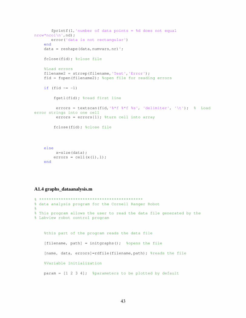
fprintf(1,'number of data points = %d does not equal nrow*ncol\n',nd); error('data is not rectangular') end data = reshape(data,numvars,nr)'; fclose(fid); %close file %Load errors filename2 = strrep(filename,'Test','Error'); fid = fopen(filename2); %open file for reading errors if (fid ~= -1) fgetl(fid); %read first line errors = textscan(fid,'%*f %*f %s', 'delimiter', '\t'); % Load error strings into one cell errors = errors{1}; %turn cell into array fclose(fid); %close file else x=size(data); errors = cell(x(1),1); end
A1.4 graphs_dataanalysis.m
% ******************************************* % data analysis program for the Cornell Ranger Robot % % This program allows the user to read the data file generated by the % Labview robot control program %this part of the program reads the data file [filename, path] = initgraphs(); %opens the file [name, data, errors]=rdfile(filename,path); %reads the file %Variable Initialization param = [1 2 3 4]; %parameters to be plotted by default
43

E=16; %variable where error is read, this value is determined by the data channel that reads the error signal err=0; %Error messages not shown at startup position = 0; %this saves the window size/position single_cursor=1; %flag to have one or multiple cursors zn=0; %zoom counter zyn=0; %zoom counter %one data point every 16 ms: T=16; %left or right arrow keys move the cursor T ms left or right: LRdelta=T; n=length(param); %create time array: index_array=1:length(data(:,1)); %array of indexes time = (index_array-1).*T ; %if T=16, time = [0 16 32 48 64 .... ] tmin = min(time); tmax = max(time); ZF=round(tmax-tmin/5); %zoom factor (variable) %corresponding array indexes for tmin and tmax: xmin = floor(tmin/T) + 1; xmax = floor(tmax/T) + 1; %save original param if user want to go back to original plot after zooming tmin_original = tmin; tmax_original = tmax; %save original data if user wants to go back after scaling data_original=data; %create mins and maxs for each parameter for f=1:25 entirerange=data(:,f); ymax(f)=max(entirerange(xmin:xmax)) + 0.05*(max(entirerange(xmin:xmax))-min(entirerange(xmin:xmax))) ; ymin(f)=min(entirerange(xmin:xmax)) - 0.05*(max(entirerange(xmin:xmax))-min(entirerange(xmin:xmax))) ; if(ymin(f)==ymax(f)) %extreme case ymax(f)=ymax(f)+1; ymin(f)=ymin(f)-1; end ZFy(f)=round(ymax(f)-ymin(f)/5); %zoom factor
44

ymax_original(f)=ymax(f); ymin_original(f)=ymin(f); ymaxd_original(f)=ymax(f); %original data max and min ymind_original(f)=ymin(f); end fig = figure(1); if (position ~= 0)%update position of figure window set(fig, 'Position', position); end %define help message as cell array of strings: helpstring{1} = 'C: change variables'; helpstring{2} = 'P: view variable names and corresponding numbers'; helpstring{3} = 'T: move the cursor to an exact time'; helpstring{4} = 'E: revert to original zoom conditions'; helpstring{5} = 'N: view new data file'; helpstring{6} = 'M: change the max and min t values (zoom in t)'; helpstring{7} = 'Y: change the max and min values for a given parameter (zoom in y)'; %helpstring{7} = 'A: toggle multiple cursor lines *cannot scroll if multiple cursors are on*'; helpstring{8} = 'O: enter a function to the data and plot the result against time'; helpstring{9} = 'U: plot 2 parameters against each other'; helpstring{10} = 'D: plot 2 or more parameters against time on the same graph'; helpstring{11} = 'L: scale a parameter'; helpstring{12} = 'R: Show Error at t'; helpstring{13} = 'B: revert to original data'; helpstring{14} = 'ARROW KEYS: scroll using left and right, zoom in x using up and down'; helpstring{15} = 'X and Z: zoom in y using this keys'; %loop initializations: but=0; t = tmin + T; x_index = round(t/T) + 1; while(but~=3) %always wait for a click %stops program by right-clicking for i = 1:length(name) %create the variable list for reference paramslist(i) = {[num2str(i),' = ',name{i},';']}; end clf; %clear current figure %This part of the program plots the data for f=1:n
45

subplot(n,1,f) %work on specific plot per iteration if(single_cursor==1) %user chose to have only one cursor %replot graphs: (erasing previous cursor) %Comment or uncomment line to plot with lines or points %plot(time,data(:,param(f)),'.','MarkerSize',4) %plots with marker points plot(time,data(:,param(f)),'','LineWidth',2) %plots with lines axis([tmin tmax ymin(param(f)) ymax(param(f))]) end if (f == 1) %display this message on the top of the window title('Press H for help'); end %plot new cursor line: t_click=[t t]; %x intercept of line (obtained from mouse click) yy=[ymin(param(f)) ymax(param(f))]; %initial y range of line for particular subplot line(t_click,yy,'Color','r') %data value display: (y vaues) text(t,ymax(param(f)), num2str(data(x_index,param(f))),... 'Tag','Cursor',... 'UserData', 4,... 'FontSize',10,... 'HorizontalAlignment','center',... 'VerticalAlignment','bottom',... 'Color','y',... 'BackgroundColor',[26/255 133/255 5/255],... 'Clipping','off',... 'ButtonDownFcn',{@CursorButtonDownFcn}); %Error display: (on error variable) if(param(f)==E) %variable where error info is located text(t,ymax(param(f))+0.3*(ymax(param(f))-ymin(param(f))), errors(x_index),... 'Tag','Cursor',.. . 'UserData', 4,... 'FontSize',10,... 'HorizontalAlignment','center',... 'VerticalAlignment','bottom',... 'Color','y',... 'BackgroundColor',[1/255 1/255 1/255],... 'Clipping','off',... 'ButtonDownFcn',{@CursorButtonDownFcn}); end %Error display: (on top)
46

if(f==1) if (err == 1) text(t,ymax(param(f))+0.35*(ymax(param(f))-ymin(param(f))), errors(x_index),... 'Tag','Cursor',... 'UserData', 4,... 'FontSize',10,... 'HorizontalAlignment','center',... 'VerticalAlignment','bottom',... 'Color','y',... 'BackgroundColor',[1/255 1/255 1/255],... 'Clipping','off',... 'ButtonDownFcn',{@CursorButtonDownFcn}); end end %data value display: (time value) if(f==n) %only for last graph text(t,ymin(param(f))-0.5*(ymax(param(f))-ymin(param(f))), ['t= ' num2str(t) ' ms'],... 'Tag','Cursor',.. . 'UserData', 4,... 'FontSize',10,... 'HorizontalAlignment','center',... 'VerticalAlignment','bottom',... 'Color','y',... 'BackgroundColor',[1/255 1/255 1/255],... 'Clipping','off',... 'ButtonDownFcn',{@CursorButtonDownFcn}); end %add appropriate variable name and index to y axis ylabel([(param(f)) name(param(f))]); end %--------------------------------button functions---------------------------------------% %get click and save x,y [t_all,y,but]=ginput(1); %t_all is in ms %change data set if (but == double('n')) position = get(fig, 'Position'); %save figure position (user may have changed it) [filename, path] = initgraphs(); if (filename ~= 0) %user did not press cancel close(gcf); [name, data]=rdfile(filename,path); %one data point every 16 ms: T=16;
47

%left or right arrow keys move the cursor 50 ms left or right: LRdelta=T; n=length(param); %create time array: index_array=1:length(data(:,1)); %array of indexes time = (index_array-1).*T ; %if T=16, time = [0 16 32 48 64 .... ] tmin = min(time); tmax = max(time); ZF=round(tmax-tmin/5); %zoom factor (variable) %corresponding array indexes for tmin and tmax: xmin = floor(tmin/T) + 1; xmax = floor(tmax/T) + 1; %save original param if user want to go back to original plot after zooming tmin_original = tmin; tmax_original = tmax; but=0; t = tmin + T; x_index = round(t/T) + 1; %create mins and maxs for each parameter for f=1:25 entirerange=data(:,f); ymax(f)=max(entirerange(xmin:xmax)); ymin(f)=min(entirerange(xmin:xmax)); if(ymin(f)==ymax(f)) %extreme case ymax(f)=ymax(f)+1; ymin(f)=ymin(f)-1; end ymax_original(f)=ymax(f); ymin_original(f)=ymin(f); end end end %changing variables to plot if (but == double('c')) msg = msgbox(paramslist, 'Variables and Values', 'modal'); %create default answer (current variables) str = [num2str(param(1)), ','];
48

for i = 2:n str = [str, num2str(param(i)), ',']; end newparamcell = inputdlg('Enter new parameter values seperated by commas:', 'Change parameters', 1, cellstr(str)); if(isempty(newparamcell)) %user pressed cancel newparamcell = cellstr(str); end close(msg) param = str2num(newparamcell{1}); n = length(param); end %changing time max,min using m key if (but == double('m')) prompt = {'New min:','New max:'}; def = {num2str(tmin),num2str(tmax)}; maxmincell = inputdlg(prompt,'Change xmax and xmin (milliseconds)', 1, def); if (isempty(maxmincell))%user pressed cancel maxmincell = def; end newmin = str2num(maxmincell{1}); newmax = str2num(maxmincell{2}); if (newmin >= newmax) %do nothing newmin = tmin; newmax = tmax; end tmin = newmin; tmax = newmax; end %user wants to bring up quick guide (help box) if (but == double('h')) uiwait(msgbox(helpstring, 'Quick Guide', 'help')); end %if user wants to list variables if (but == double('p')) uiwait(msgbox(paramslist, 'Variables and Values')) end %moving cursor conditions: if(but==1)%left click %save useful mouse location data only when user left-clicks: t = round(t_all); x_index = round(t/T) + 1; end %user wants to move cursor left if(but==28) %but=28 ==> left arrow key pressed newt = t - LRdelta; if (newt >= 0) %ensure t is nonnegative if (newt < tmin) %move plot to the right, since cursor can't move further left
49

tmin = newt; tmax = tmax - LRdelta; end t = newt; end x_index = round(t/T) + 1; end %user wants to move cursor right if(but==29) %but=29 ==> right arrow key pressed newt=t+LRdelta; if (newt <= max(time)) %ensure t is within domain if (newt > tmax) %move plot to the left, since cursor can't move further right tmax = newt; tmin = tmin + LRdelta; end t = newt; end x_index = round(t/T) + 1; end % move cursor by directly entering new value if (but == double('t')) newxcell = inputdlg('Input time value:','View Input Time',1,cellstr(num2str(t))); newt = str2double(newxcell{1}); if(newt < tmin && newt >= min(time)) tmin = newt; elseif(newt > tmax && newt <= max(time)) tmax = newt; end if (newt >= min(time) && newt <= max(time)) t = newt; x_index = round(t/T) + 1; end end %zooming conditions: %user wants to zoom in but=30 ==> up arrow key pressed if(but==30) zn=zn+1; tmin=t-ZF/zn; tmax=t+ZF/zn; end %user wants to zoom out but=31 ==> down arrow key pressed if(but==31) if(zn>1) %removes case of dividing by zero zn=zn-1; tmin=t-ZF/zn; tmax=t+ZF/zn; end end
50

%user wants to zoom in in y if(but==double('x')) zyn=zyn+1; ymin=data(x_index,1:25)-ZFy./zyn; ymax=data(x_index,1:25)+ZFy./zyn; end %user wants to zoom out in y if(but==double('z')) if(zyn>1) %removes case of dividing by zero zyn=zyn-1; ymin=data(x_index,1:25)-ZFy./zyn; ymax=data(x_index,1:25)+ZFy./zyn; end end %user wants stop zooming and go back to original graph if(but== double('e')) tmin=tmin_original; tmax=tmax_original; ymin=ymin_original; ymax=ymax_original; zn=1; end %manipulate the data and plot the result against time if (but == double('o')) mandata=input('introduce an expression to compute the parameter with >>'); ymaxm=max(mandata(xmin:xmax)); yminm=min(mandata(xmin:xmax)); if(yminm==ymaxm) %extreme case ymaxm=ymaxm+1; yminm=yminm-1; end figure axis([tmin tmax yminm ymaxm]) plot(time,mandata,'','LineWidth',2) grid on figure(1) end %Plot 2 parameters against each other if (but == double('u')) msg = msgbox(paramslist, 'Variables and Values', 'modal'); paramx = inputdlg('Enter parameter to be plotted on x axis:', 'Plot 2 parameters against each other', 1);
51

paramy = inputdlg('Enter parameter to be plotted on y axis:', 'Plot 2 parameters against each other', 1); graphtitle = inputdlg('Enter title for your graph', 'Plot 2 parameters against each other', 1); if(isempty(paramx)) %user pressed cancel paramx = '1'; end if(isempty(paramy)) %user pressed cancel paramy = '1'; end xparam = str2double(paramx); yparam = str2double(paramy); figure plot(data(:,xparam),data(:,yparam)) title(graphtitle) xlabel(name(xparam)) ylabel(name(yparam)) grid on close(msg ) figure(1) end %plot 2 or more parameters against time if (but == double('d')) msg = msgbox(paramslist, 'Variables and Values', 'modal'); %create default answer (current variables) str = [num2str(param(1)), ',']; for k = 2:n str = [str, num2str(param(k)), ',']; end paramplotstr = inputdlg('Enter parameters to be plotted:', 'Plot more than one parameter vs. time on graph', 1,cellstr(str)); %paramplot = input('Enter parameters to be plotted:'); graphtitle = inputdlg('Enter title for your graph', 'Plot more than one parameter vs. time on graph', 1); paramplot = str2num(paramplotstr{1}); close(msg) figure for k=1:length(paramplot)
52

%plot(time,data(:,paramplot(k)),'.','MarkerSize',4) %plots with marker points h=plot(time,data(:,paramplot(k)),'','LineWidth',2); %plots with lines title(graphtitle) grid on hold all end legend(name(paramplot(1:length(paramplot))),'Location', 'SO') figure(1) end %zoom in y if (but == double('y')) msg = msgbox(paramslist, 'Variables and Values', 'modal'); paramminmax = inputdlg('Enter number of parameter to be zoomed:', 'Zoom on y axis', 1); i = str2double(paramminmax); yprompt = {'New min:','New max:'}; def = {num2str(ymin(i)),num2str(ymax(i))}; ymaxmincell = inputdlg(yprompt,'Change ymax and ymin', 1, def); if (isempty(ymaxmincell))%user pressed cancel ymaxmincell = def; end ynewmin = str2num(ymaxmincell{1}); ynewmax = str2num(ymaxmincell{2}); if (ynewmin >= ynewmax) %do nothing ynewmin = ymin(i); ynewmax = ymax(i); end ymin(i) = ynewmin; ymax(i) = ynewmax; close(msg) end %scale parameters if (but == double('l')) msg = msgbox(paramslist, 'Variables and Values', 'modal'); scprompt = {'Parameter to scale:','Scale factor:'}; paramscale = inputdlg(scprompt, 'Scale a parameter', 1);
53

if (isempty(paramscale))%user pressed cancel paramscale = {'1','1'}; end pscale=str2double(paramscale{1}); scale=str2double(paramscale{2}); close(msg) data(:,pscale) = scale*data(:,pscale); entirerange=data(:,pscale); ymax(pscale)=max(entirerange(xmin:xmax)); ymin(pscale)=min(entirerange(xmin:xmax)); if(ymin(pscale)==ymax(pscale)) %extreme case ymax(pscale)=ymax(pscale)+1; ymin(pscale)=ymin(pscale)-1; end ZFy(pscale)=round(ymax(pscale)-ymin(pscale)/5); %zoom factor ymax_original(pscale)=ymax(pscale); %new original zoom conditions for the parameter ymin_original(pscale)=ymin(pscale); end %go back to original data if(but== double('b')) tmin=tmin_original; tmax=tmax_original; ymin=ymind_original; ymax=ymaxd_original; ymin_original=ymind_original; ymax_original=ymaxd_original; data=data_original; zn=1; end %show (and stop showing) errors on top of the page if (but == double('r')) err=1; end if (but == double('f')) err=0; end
54

%------------------------end button functions------------------------% %limit x-axis: if(tmin<0) tmin=0; end %mm=length( data(:,param(2)) ); if(tmax> max(time)) tmax=max(time); end end %while
A1.5 graphs_videoread.m
% ******************************************* % data and video analysis program for the Cornell Ranger Robot % % This program allows the user to read the data file generated by the % Labview robot control program plus a video of any format clear all clear fig %Prompt user for data file and read it [filename, path] = initgraphs(); [name, data, errors]=rdfile(filename,path); %prompt user for video file: [vfilename, vpath] = uigetfile('*.*', 'Choose Video File'); addpath(vpath); cd(vpath) %read video file. The usual maximum frames that the program can read is %about 600 movread = mmread(vfilename,[],[],false,true); %get parameters from the video file maxframes=movread.nrFramesTotal; %number of frames mov=movread.frames; %frame info h=movread.height; %height of video w=movread.width; %width of video
55

%Variable initialization param = [1 2 3 4]; E=16; %variable where error is read err=0; position = 0; %this saves the window size/position single_cursor=1; %flag to have one or multiple cursors Gmode=0; %flag to toggle between Graph only and Graph+Video modes -- intitially in Graph+Video %Synchronize=0; Gmode_change=1; zn=0; %zoom counter zyn=0; %zoom counter %camera frame rate: FPS=round(movread.rate); %frames per second from camera. edit if value is incorrect %get the period automatically from reading the time stamp in the data %file: T=data(3,1) - data(2,1); %originally T=16ms %T=1; %left or right arrow keys move the cursor LRdelta ms left or right: LRdelta=round(1000/FPS); %time between two camera frames (camera mode) ----> is rounding good ???? n=length(param); %create time array: index_array=1:length(data(:,1)); %array of indexes time = (index_array-1).*T ; %if T=16, time = [0 16 32 48 64 .... ] tmin = min(time); tmax = max(time); ZF=round(tmax-tmin/5); %zoom factor (variable) %corresponding array indexes for tmin and tmax: xmin = floor(tmin/T) + 1; xmax = floor(tmax/T) + 1; c=1; %save original param if user want to go back to original plot after zooming tmin_original = tmin;
56

tmax_original = tmax; %save original data if user wants to go back after scaling data_original=data; %create mins and maxs for each parameter for f=1:25 entirerange=data(:,f); ymax(f)=max(entirerange(xmin:xmax)) + 0.05*(max(entirerange(xmin:xmax))-min(entirerange(xmin:xmax))) ; ymin(f)=min(entirerange(xmin:xmax)) - 0.05*(max(entirerange(xmin:xmax))-min(entirerange(xmin:xmax))) ; if(ymin(f)==ymax(f)) %extreme case ymax(f)=ymax(f)+1; ymin(f)=ymin(f)-1; end ZFy(f)=round(ymax(f)-ymin(f)/5); %zoom factor ymax_original(f)=ymax(f); ymin_original(f)=ymin(f); ymaxd_original(f)=ymax(f); %original data max and min ymind_original(f)=ymin(f); end %intialize variables to save synchronization points k_sync=1; t_sync=tmin+T; x_sync = round(t_sync/T) + 1; %initialize variables for video file: play_speed=15; k=1; loc=[0.5 0.5 0 0]; nmovie=[1 k]; but=0; Allow=0; play=0; Fwd=0; moveright=0; fig2=figure(2);
57

set(fig2,'Position', [5 100 w h+30]) %screen buttons: hR = uicontrol(fig2,'Style', 'pushbutton', 'String', 'right',... 'Position', [55 h 50 30], 'Callback', 'but=29'); hL = uicontrol(fig2,'Style', 'pushbutton', 'String' 'left',... , 'Position', [5 h 50 30], 'Callback', 'but=28'); hS = uicontrol(fig2,'Style', 'pushbutton', 'String', 'Load New Data File',... 'Position', [210 h 100 30], 'Callback', 'but=110'); hA = uicontrol(fig2,'Style', 'pushbutton', 'String', 'Allow Graph functions',... 'Position', [430 h 120 30], 'Callback', 'Allow=1'); hP = uicontrol(fig2,'Style', 'pushbutton', 'String', 'Play',... 'Position', [110 h 50 30], 'Callback', 'play=1'); hS = uicontrol(fig2,'Style', 'pushbutton', 'String', 'Stop',... 'Position', [160 h 50 30], 'Callback', 'play=0'); hGr = uicontrol(fig2,'Style', 'pushbutton', 'String', 'Go to data window',... 'Position', [310 h 120 30], 'Callback', 'Gmode=1'); hFwd = uicontrol(fig2,'Style', 'slider','value',1,... 'SliderStep',[1/maxframes 0.1],'min',1,'max',maxframes,... 'Position', [0 0 w 20], 'Callback', 'Fwd=1'); hfps= uicontrol(fig2,'Style','edit ...%,'Min',1,'Max',200)%... ', 'Position',[0 20 30 20]) % uicontrol(hR) uicontrol(hL) uicontrol(hS) uicontrol(hA) uicontrol(hP) uicontrol(hS) uicontrol(hGr) uicontrol(hFwd) %Data window fig = figure(1); if (position ~= 0)%update position of figure window set(fig, 'Position', position); end %define help message as cell array of strings: helpstring{1} = 'C: change variables'; helpstring{2} = 'P: view variable names and corresponding numbers'; helpstring{3} = 'T: move the cursor to an exact time'; helpstring{4} = 'E: revert to original zoom conditions'; helpstring{5} = 'N: view new data file'; helpstring{6} = 'M: change the max and min t values (zoom in t)';
58

helpstring{7} = 'Y: change the max and min values for a given parameter (zoom in y)'; %helpstring{7} = 'A: toggle multiple cursor lines *cannot scroll if multiple cursors are on*'; helpstring{8} = 'O: enter a function to the data and plot the result against time'; helpstring{9} = 'U: plot 2 parameters against each other'; helpstring{10} = 'D: plot 2 or more parameters against time on the same graph'; helpstring{11} = 'L: scale a parameter'; helpstring{12} = 'R: Show Error at t'; helpstring{13} = 'B: revert to original data'; helpstring{14} = 'ARROW KEYS: scroll using left and right, zoom in x using up and down'; helpstring{15} = 'X and Z: zoom in y using this keys'; helpstring{16} = 'S: To synchronize: When in Graph Mode, move cursor to data point that corresponds with current video frame and press S'; helpstring{17} = 'V: Return to Video Mode (Synchronization will be saved)'; %loop initializations: but=0; t = tmin + T; x_index = round(t/T) + 1; x_indexmin=x_index; x_indexmax=round((tmax)/T) - 1; while(but~=3) %always wait for a click %stops program by right-clicking but=0; for i = 1:length(name) %create the variable list for reference paramslist(i) = {[num2str(i),' = ',name{i},';']}; end %limits video frames at extremes: if(nmovie(2)==0) k=1; nmovie(2)=1; end if(nmovie(2)>=maxframes) k=maxframes; nmovie(2)=maxframes; end nmovie x_index movie(fig2,mov,nmovie,play_speed,loc) %displays the video
59

set(0,'CurrentFigure',fig) % make figure 1 current figure for plotting if(but==3) disp torma!!!! ttt=333 end if(play==1 && k<maxframes) if x_index==x_indexmax msgbox('You have reached the end of the data') play=0 else k=k+1; c=1; movecursor=1; nmovie=[1 k]; moveright=1; set(hFwd,'value',k); end end if(but==28) %user wants to move cursor left but=28 ==> left arrow key pressed if (x_index==x_indexmin || x_index==(x_indexmin+1)) msgbox('You have reached the begining of the data') else c=1; movecursor=1; k=k-1; nmovie=[1 k]; set(hFwd,'value',k); end end if(but==29) %user wants to move cursor right but=29 ==> right arrow key pressed if x_index > x_indexmax-1 msgbox('You have reached the end of the data') else c=1; movecursor=1; k=k+1; nmovie=[1 k]; set(hFwd,'value',k); end end if (Fwd==1) comp=k; k=get(hFwd,'value'); k=round(k); nmovie=[1 k]; if (comp < k)
60

c=k-comp; but=29; moveright=1; end if (comp > k) c=comp-k; but=28; end Fwd=0; end %this part of the program plots the data for f=1:n subplot(n,1,f) %work on specific plot per iteration if(single_cursor==1) %user chose to have only one cursor %replot graphs: (erasing previous cursor) %Comment or uncomment line to plot with lines or points plot(time,data(:,param(f)),'.','MarkerSize',4) %plots with marker points %plot(time,data(:,param(f)),'','LineWidth',2) %plots with %lines axis([tmin tmax ymin(param(f)) ymax(param(f))]) end if (f == 1) %display this message on the top of the window title('Press H for help'); end %plot new cursor line: t_click=[t t]; %x intercept of line (obtained from mouse click) yy=[ymin(param(f)) ymax(param(f))]; %initial y range of line for particular subplot line(t_click,yy,'Color','r') %data value display: (y vaues) text(t,ymax(param(f)), num2str(data(x_index,param(f))),... 'Tag','Cursor',... 'UserData', 4,... 'FontSize',10,... 'HorizontalAlignment','center',... 'VerticalAlignment','bottom',... 'Color','y',... 'BackgroundColor',[26/255 133/255 5/255],...
61

'Clipping','off',... 'ButtonDownFcn',{@CursorButtonDownFcn}); %Error display: (on error variable) if(param(f)==E) %variable where error info is located text(t,ymax(param(f))+0.3*(ymax(param(f))-ymin(param(f))), errors(x_index),... 'Tag','Cursor',... 'UserData', 4,... 'FontSize',10,... 'HorizontalAlignment','center',... 'VerticalAlignment','bottom',... 'Color','y',... 'BackgroundColor',[1/255 1/255 1/255],... 'Clipping','off',... 'ButtonDownFcn',{@CursorButtonDownFcn}); end %Error display: (on top) if(f==1) if (err == 1) text(t,ymax(param(f))+0.35*(ymax(param(f))-ymin(param(f))), errors(x_index),... 'Tag','Cursor',... 'UserData', 4,... 'FontSize',10,... 'HorizontalAlignment','center',... 'VerticalAlignment','bottom',... 'Color','y',... 'BackgroundColor',[1/255 1/255 1/255],... 'Clipping','off',... 'ButtonDownFcn',{@CursorButtonDownFcn}); end end %data value display: (time value) if(f==n) %only for last graph text(t,ymin(param(f))-0.5*(ymax(param(f))-ymin(param(f))), ['t= ' num2str(t) ' ms'],... 'Tag','Cursor',... 'UserData', 4,... 'FontSize',10,... 'HorizontalAlignment','center',... 'VerticalAlignment','bottom',... 'Color','y',... 'BackgroundColor',[1/255 1/255 1/255],... 'Clipping','off',... 'ButtonDownFcn',{@CursorButtonDownFcn}); end %add appropriate variable name and index to y axis ylabel([(param(f)) name(param(f))]); end %--------------------------------button functions---------------------------------------%
62

if(Gmode==0) %Graph+Vide0 mode LRdelta=round(1000/FPS); %vertical cursor moves left or right by period between two video frames Gmode_change=1; end if(Gmode==1) %graph only mode LRdelta=T; %vertical cursor moves left or right by period between two data points disp GraphMode! if(Gmode_change==1) uiwait(msgbox('You can now use Graph functions. Press H for help or S to synchronize a data point with current video frame. Press V to return to video mode', 'Graph mode')) Gmode_change=0; end [t_all,y,but]=ginput(1); %t_all is in ms %always waits for keyboard or mouse commands end if(Allow==1) %can also get graphs keyboard or mouse for graphs while in video mode disp GnputAllowed!!! [t_all,y,but]=ginput(1); %t_all is in ms Allow=0; end %go back to video mode if(but == double('v')) Gmode=0; k=k_sync; %return to saved framd and data point number when synchronized x_index=x_sync; t=t_sync; uiwait(msgbox('Successfully returned to Video Mode at synchronized point', 'Success')) end %change data set if (but == double('n')) position = get(fig, 'Position'); %save figure position (user may have changed it) [filename, path] = initgraphs(); if (filename ~= 0) %user did not press cancel [name, data, errors]=rdfile(filename,path); T=data(3,1) - data(2,1); %originally T=16ms
63

%left or right arrow keys move the cursor LRdelta ms left or right: LRdelta=round(1000/FPS); %time between two camera frames (camera mode %create time array: index_array=1:length(data(:,1)); %array of indexes time = (index_array-1).*T ; %if T=16, time = [0 16 32 48 64 .... ] tmin = min(time); tmax = max(time); ZF=round(tmax-tmin/5); %zoom factor (variable) %corresponding array indexes for tmin and tmax: xmin = floor(tmin/T) + 1; xmax = floor(tmax/T) + 1; %save original param if user want to go back to original plot after zooming tmin_original = tmin; tmax_original = tmax; but=0; t = tmin + T; x_index = round(t/T) + 1; %create mins and maxs for each parameter for f=1:25 entirerange=data(:,f); ymax(f)=max(entirerange(xmin:xmax)); ymin(f)=min(entirerange(xmin:xmax)); if(ymin(f)==ymax(f)) %extreme case ymax(f)=ymax(f)+1; ymin(f)=ymin(f)-1; end ymax_original(f)=ymax(f); ymin_original(f)=ymin(f); end end end %changing variables to plot if (but == double('c')) msg = msgbox(paramslist, 'Variables and Values', 'modal'); %create default answer (current variables) str = [num2str(param(1)), ','];
64

for i = 2:n str = [str, num2str(param(i)), ',']; end newparamcell = inputdlg('Enter new parameter values seperated by commas:', 'Change parameters', 1, cellstr(str)); if(isempty(newparamcell)) %user pressed cancel newparamcell = cellstr(str); end close(msg) param = str2num(newparamcell{1}); n = length(param); end %changing time max,min using m key if (but == double('m')) prompt = {'New min:','New max:'}; def = {num2str(tmin),num2str(tmax)}; maxmincell = inputdlg(prompt,'Change xmax and xmin (milliseconds)', 1, def); if (isempty(maxmincell))%user pressed cancel maxmincell = def; end newmin = str2num(maxmincell{1}); newmax = str2num(maxmincell{2}); if (newmin >= newmax) %do nothing newmin = tmin; newmax = tmax; end tmin = newmin; tmax = newmax; end %user wants to bring up quick guide (help box) if (but == double('h')) uiwait(msgbox(helpstring, 'Quick Guide', 'help')); end %user wants to synchronize data and video if (but == double('s')) k_sync=k; %save current frame and data point number x_sync=x_index; t_sync=t; k_str=num2str(k); x_str=num2str(x_index); uiwait(msgbox(['Video and Graph successfully synchronized: Frame No ',k_str,' with Data Point No ',x_str,], 'Success', 'Sync')); end %if user wants to list variables if (but == double('p')) uiwait(msgbox(paramslist, 'Variables and Values')) end
65

%------------------------------------------------------------------ %------------------------------------------------------------------ %moving cursor conditions: if(but==1)%left click %save useful mouse location data only when user left-clicks: t = round(t_all); x_index = round(t/T) + 1; end %user wants to move cursor left if(but==28) %but=28 ==> left arrow key pressed newt = t - c*LRdelta; if (newt >= 0) %ensure t is nonnegative if (newt < tmin) %move plot to the right, since cursor can't move further left tmin = newt; tmax = tmax - LRdelta; end t = newt; end x_index = round(t/T) + c; end %user wants to move cursor right if(but==29 || moveright==1) %but=29 ==> right arrow key pressed moveright=0; newt=t+ c*LRdelta; if (newt <= max(time)) %ensure t is within domain if (newt > tmax) %move plot to the left, since cursor can't move further right tmax = newt; tmin = tmin + LRdelta; end t = newt; end x_index = round(t/T) + 1; end % move cursor by directly entering new value if (but == double('t')) newxcell = inputdlg('Input time value:','View Input Time',1,cellstr(num2str(t))); newt = str2double(newxcell{1}); if(newt < tmin && newt >= min(time)) tmin = newt; elseif(newt > tmax && newt <= max(time)) tmax = newt; end if (newt >= min(time) && newt <= max(time)) t = newt; x_index = round(t/T) + 1;
66

end end %zooming conditions: %user wants to zoom in time but=30 ==> up arrow key pressed if(but==30) zn=zn+1; tmin=t-ZF/zn; tmax=t+ZF/zn; end %user wants to zoom out time but=31 ==> down arrow key pressed if(but==31) if(zn>1) %removes case of dividing by zero zn=zn-1; tmin=t-ZF/zn; tmax=t+ZF/zn; end end %user wants to zoom in in y if(but==double('x')) zyn=zyn+1; ymin=data(x_index,1:25)-ZFy./zyn; ymax=data(x_index,1:25)+ZFy./zyn; end %user wants to zoom out in y if(but==double('z')) if(zyn>1) %removes case of dividing by zero zyn=zyn-1; ymin=data(x_index,1:25)-ZFy./zyn; ymax=data(x_index,1:25)+ZFy./zyn; end end %user wants stop zooming and go back to original graph if(but== double('e')) tmin=tmin_original; tmax=tmax_original; ymin=ymin_original; ymax=ymax_original; zn=1; end %manipulate the data and plot the result against time if (but == double('o')) mandata=input('introduce an expression to compute the parameter with >>'); ymaxm=max(mandata(xmin:xmax)); yminm=min(mandata(xmin:xmax));
67

if(yminm==ymaxm) %extreme case ymaxm=ymaxm+1; yminm=yminm-1; end figure(3) axis([tmin tmax yminm ymaxm]) plot(time,mandata,'','LineWidth',2) grid on figure(1) end %Plot 2 parameters against each other if (but == double('u')) msg = msgbox(paramslist, 'Variables and Values', 'modal'); paramx = inputdlg('Enter parameter to be plotted on x axis:', 'Plot 2 parameters against each other', 1); paramy = inputdlg('Enter parameter to be plotted on y axis:', 'Plot 2 parameters against each other', 1); graphtitle = inputdlg('Enter title for your graph', 'Plot 2 parameters against each other', 1); if(isempty(paramx)) %user pressed cancel paramx = '1'; end if(isempty(paramy)) %user pressed cancel paramy = '1'; end xparam = str2double(paramx); yparam = str2double(paramy); figure(3) plot(data(:,xparam),data(:,yparam)) title(graphtitle) xlabel(name(xparam)) ylabel(name(yparam)) grid on close(msg) figure(1) end %plot 2 or more parameters against time if (but == double('d'))
68

msg = msgbox(paramslist, 'Variables and Values', 'modal'); %create default answer (current variables) str = [num2str(param(1)), ',']; for k = 2:n str = [str, num2str(param(k)), ',']; end paramplotstr = inputdlg('Enter parameters to be plotted:', 'Plot more than one parameter vs. time on graph', 1,cellstr(str)); graphtitle = inputdlg('Enter title for your graph', 'Plot more than one parameter vs. time on graph', 1); paramplot = str2num(paramplotstr{1}); close(msg) figure(3) for k=1:length(paramplot) %plot(time,data(:,paramplot(k)),'.','MarkerSize',4) %plots with marker points h=plot(time,data(:,paramplot(k)),'','LineWidth',2); %plots with lines title(graphtitle) grid on hold all end legend(name(paramplot(1:length(paramplot))),'Location', 'SO') figure(1) end %zoom in y if (but == double('y')) msg = msgbox(paramslist, 'Variables and Values', 'modal'); paramminmax = inputdlg('Enter number of parameter to be zoomed:', 'Zoom on y axis', 1); i = str2double(paramminmax); yprompt = {'New min:','New max:'}; def = {num2str(ymin(i)),num2str(ymax(i))}; ymaxmincell = inputdlg(yprompt,'Change ymax and ymin', 1, def); if (isempty(ymaxmincell))%user pressed cancel ymaxmincell = def;
69

end ynewmin = str2num(ymaxmincell{1}); ynewmax = str2num(ymaxmincell{2}); if (ynewmin >= ynewmax) %do nothing ynewmin = ymin(i); ynewmax = ymax(i); end ymin(i) = ynewmin; ymax(i) = ynewmax; close(msg) end %scale parameters if (but == double('l')) msg = msgbox(paramslist, 'Variables and Values', 'modal'); scprompt = {'Parameter to scale:','Scale factor:'}; paramscale = inputdlg(scprompt, 'Scale a parameter', 1); if (isempty(paramscale))%user pressed cancel paramscale = {'1','1'}; end pscale=str2double(paramscale{1}); scale=str2double(paramscale{2}); close(msg) data(:,pscale) = scale*data(:,pscale); entirerange=data(:,pscale); ymax(pscale)=max(entirerange(xmin:xmax)); ymin(pscale)=min(entirerange(xmin:xmax)); if(ymin(pscale)==ymax(pscale)) %extreme case ymax(pscale)=ymax(pscale)+1; ymin(pscale)=ymin(pscale)-1; end ZFy(pscale)=round(ymax(pscale)-ymin(pscale)/5); %zoom factor ymax_original(pscale)=ymax(pscale); %new original zoom conditions for the parameter ymin_original(pscale)=ymin(pscale); end %go back to original data if(but== double('b')) tmin=tmin_original; tmax=tmax_original;
70

71
ymin=ymind_original; ymax=ymaxd_original; ymin_original=ymind_original; ymax_original=ymaxd_original; data=data_original; zn=1; end %show (and stop showing) errors on top of the page if (but == double('r')) err=1; end if (but == double('f')) err=0; end %------------------------end button functions------------------------% %limit x-axis: if(tmin<0) tmin=0; end if(tmax> max(time)) tmax=max(time); end end %while % run graphs7scrE
Top Related