


Languages
Pages
Legal


CLINICAL DOSIMETRY IN
RADIOTHERAPY
Karl L. Prado, Ph.D., FACR, FAAPM
Argonne National Laboratory Course: 3DCRT for Technologists
Department of Radiation Oncology

Advertencia:

Dose Ratios and MU Calculations
Our Goals:
A. Actually understand
things like PDDs,
Inverse Square,
TMRs, Scatter
Factors, and other
such physics terms …
B. And then be able to
use them in
calculations of
accelerator monitor-
units
Not as scary as you think!

Objectives
Understand the basic concepts underlying radiation
dosimetry
Recognize the fundamental quantities that are used
to describe these basic radiation dosimetry concepts
Apply radiation dosimetry concepts and quantities
in calculations of dose in clinical radiation-oncology
practice situations

Clinical Dosimetry
Fundamental Quantities
Think measurements
made in a water
phantom
Define quantities: the
ratio of doses at two
points: one point
different than the other
because of distance,
depth, and conditions of
scatter
MU Calculations
Apply measured data
to clinical dose
calculations
Specifically – calculate
the monitor-unit setting
on the treatment unit
that will deliver an
intended dose

The next couple of hours
First talk about how we
characterize dose
deposition in a medium
… “dosimetry” (dose
ratios)
Then talk about dose-
calculation methods …
Perform an accelerator
monitor-unit (MU)
calculation

Sample Dose Calculation Problem
A patient’s whole brain is to be treated.
The prescribed dose is 300 cGy per fraction, (10
fractions, 30 Gy total dose).
Radiation and technique are 6 MV x rays, parallel-
opposed right and left lateral fields
Prescribed dose is to isocenter.
Fields are 20x18, mlc-shaped
The patient set up for isocentric treatment at mid-
brain, lateral separation 16 cm
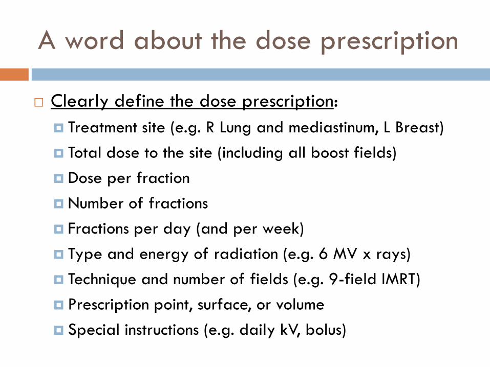
A word about the dose prescription
Clearly define the dose prescription:
Treatment site (e.g. R Lung and mediastinum, L Breast)
Total dose to the site (including all boost fields)
Dose per fraction
Number of fractions
Fractions per day (and per week)
Type and energy of radiation (e.g. 6 MV x rays)
Technique and number of fields (e.g. 9-field IMRT)
Prescription point, surface, or volume
Special instructions (e.g. daily kV, bolus)

Who else thinks this is a pretty cool
Google Logo?

Beam Data (Measured Dose Ratios)
Quantitative description of
the dose characteristics of
the therapy beams
All units
All energies
Each machine and energy
has its corresponding set of
beam data
Machine Data Book
“Golden Data Set”
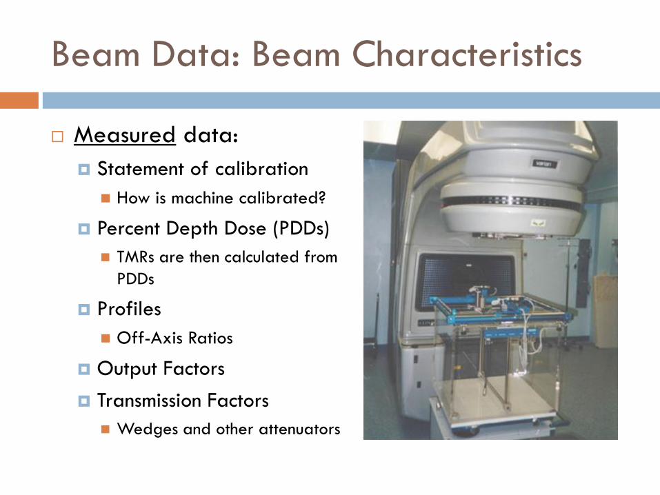
Beam Data: Beam Characteristics
Measured data:
Statement of calibration
How is machine calibrated?
Percent Depth Dose (PDDs)
TMRs are then calculated from
PDDs
Profiles
Off-Axis Ratios
Output Factors
Transmission Factors
Wedges and other attenuators

Beam Data
What’s in the
machine data
books?

The Definitions of Field Size
Many details
How defined? …
SSD, SAD
Field size at what
distance? …
beam divergence
How produced?
… collimator
jaws, multi-leaf
collimator
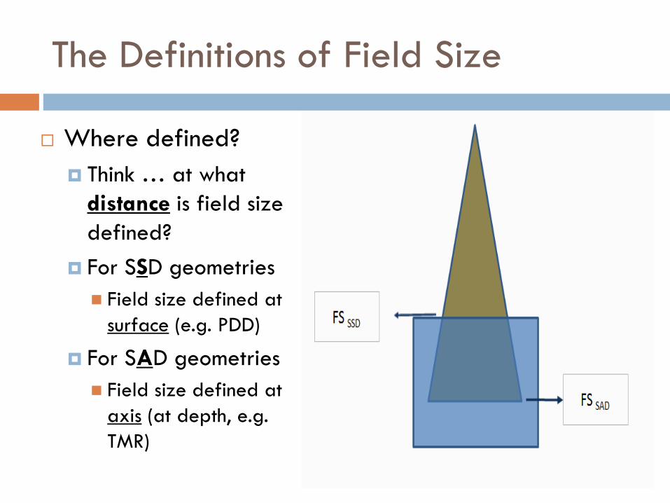
The Definitions of Field Size
Where defined?
Think … at what
distance is field size
defined?
For SSD geometries
Field size defined at
surface (e.g. PDD)
For SAD geometries
Field size defined at
axis (at depth, e.g.
TMR)
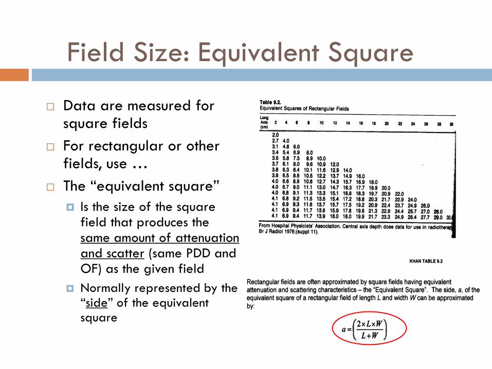
Field Size: Equivalent Square
Data are measured for square fields
For rectangular or other fields, use …
The “equivalent square”
Is the size of the square field that produces the same amount of attenuation and scatter (same PDD and OF) as the given field
Normally represented by the “side” of the equivalent square

Dose Ratios Concepts:
Distance and Depth
Distance How far away
from the source
Inverse Square
Depth How deep in
absorber (water, patient)
Attenuation
Note Difference !! Commonly
confused

Distance, Depth, and Scatter
How does the dose at
point P differ from
that at point Q?
Point P farther away
Inverse square
Point P deeper
Attenuation
Field size at Point P
larger
More scatter
Dosimetry Concepts in 1 Dimension
1D Dose Distributions

Percent Depth Dose (PDD)
PDD Notes
The differences in dose at
the two depths, d0 and d,
are due to:
Differences in depth
Differences in distance
Differences in field size at
each depth (scatter)
Field size is defined at
the surface of the
phantom or patient 0/ dd DDPDD

PDD: Depth and Energy
Dependence
PDD Curves - Characteristics
Note change in depth of dmax
Can characterize beam quality (energy) using
PDD at 10-cm depth
Build-up
Region
What leads
to Build-up
Effect?

PDD Build-up Region
Kerma to dose relationship Kerma and dose represent
two different quantities
Kerma is energy released
Dose is energy absorbed
Build-up region produced by forward-scattered electrons that stop at deeper depths
Areas under both curves are equal

PDD: Distance, Depth, Scatter
Note that in mathematical description of PDD:
Inverse-square (distance) factor
Dependence on SSD
Attenuation (depth) factor
Scatter (field-size) factor

PDD: Effect of Distance
Effect of inverse-square
term on PDD
As distance increases,
relative change in dose
rate decreases (less steep
slope)
Less Inverse-Square effect
This results in an increase in
PDD (since there is less of
a dose decrease due to
distance), although the
actual dose rate decreases

PDD Example
If the dose in a 10x10 cm2 field at
the depth of dmax in water 100 cm
SDD is 200 cGy, what is the dose
at a depth of 10 cm?
0/ dd DDPDD
PDDDD dd 0
6.133668.0200dD

The Mayneord F Factor
(no longer a mystery) The inverse-square term within the PDD
PDD is a function of distance (SSD + depth)
PDDs at given depths and distances (SSD) can be corrected to produce approximate PDDs at the same depth but at other distances by applying the Mayneord F factor
“Divide out” the previous inverse-square term (for SSD1), “multiply in” the new inverse-square term (for SSD2)
I have a patient set up at 120
cm SSD, but I only have 100
cm SSD PDD tables …

The Mayneord F Factor
Mayneord F – Example
Previous Problem
100 SSD, 10x10, depth 10
PDD was 0.668
Now assume 120 SSD …
Divide out 100 SSD, d10 inverse square, and multiply back in 120 SSD, d10 inverse square:
685.0668.0
1105.101
1305.121
2
2

TAR: A traditional yet useful quantity
The TAR …
Developed for isocentric treatments
The ratio of doses at two points:
Equidistant from the source
That have equal field sizes at the points of calculation
Field size is defined at point of calculation
Relates dose at depth to dose “in air” (free space)
Concept of “equilibrium mass”
Need for electronic equilibrium – constant Kerma-to-dose relationship
fsd DDTAR /

PSF (BSF): An extension of the TAR
The PSF (or BSF) is a special case of the TAR when dose in air is compared to dose at the depth (dmax) of maximum dose
At this point the dose is maximum (peak) since the contribution of scatter is not offset by attenuation
The term BSF applies strictly to situations where the depth of dmax occurs at the surface of the phantom or patient (i.e. kV x rays)

PSF Details: Energy and Field Size
In general, scatter contribution decreases as energy increases
Note:
Scatter can contribute as much as 50% to the dose a dmax in kV beams
The effect at 60Co is of the order of a few percent (PSF 60Co 10x10 = 1.035
Increase in dose is greatest in smaller fields (note 5x5, 10x10, and 20x20)

TPR and TMR: More current quantities
Similar to the TAR, the TPR is the ratio of doses (Dd and Dt0) at two points equidistant from the source Field sizes are equal
Again field size is defined at depth of calculation
Only attenuation by depth differs
The TMR is a special case of the TPR when t0 equals the depth of dmax
0/ td DDTPR
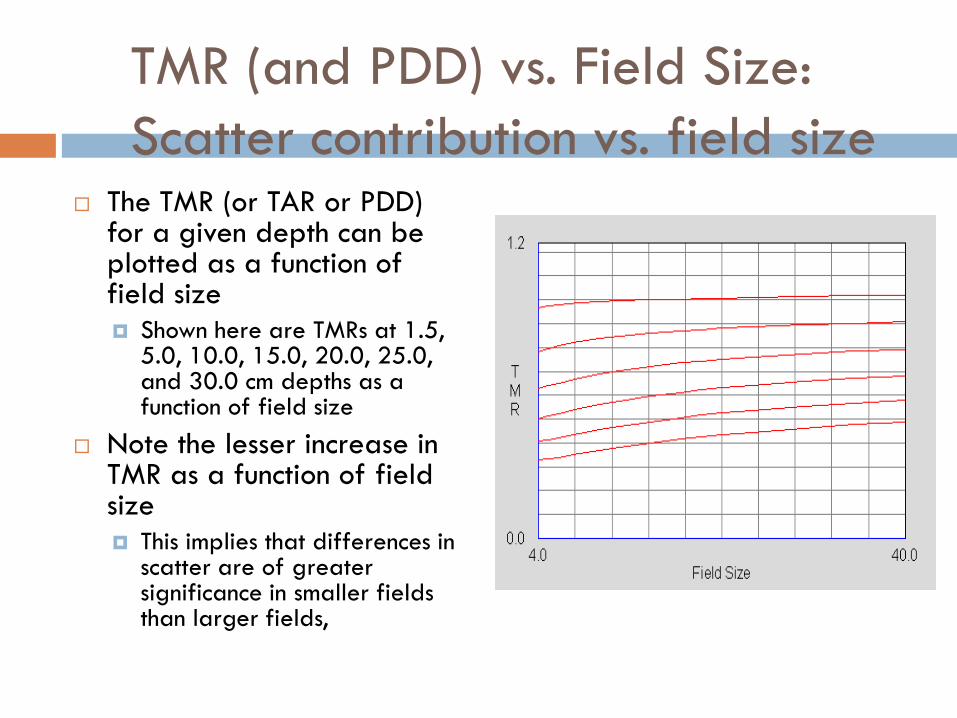
TMR (and PDD) vs. Field Size:
Scatter contribution vs. field size The TMR (or TAR or PDD)
for a given depth can be plotted as a function of field size Shown here are TMRs at 1.5,
5.0, 10.0, 15.0, 20.0, 25.0, and 30.0 cm depths as a function of field size
Note the lesser increase in TMR as a function of field size This implies that differences in
scatter are of greater significance in smaller fields than larger fields,

TMR / PDD / TAR Relationships
From: ICRU 14

TMR / PDD Relationship

Scatter Factors
Characterize scatter
Scatter factors describe field-size dependence of dose at a point Often wise to
separate sources of scatter
Scatter from the head of the treatment unit
Scatter from the phantom or patient
Measurements complicated by need for electronic equilibrium
Khan

Transmission Factors: Wedges
Beam intensity is also affected by the introduction of beam attenuators that may be used modify the beam’s shape or intensity Such attenuators may be
plastic trays used to support field-shaping blocks, or physical wedges used to modify the beam’s intensity
The transmission of radiation through attenuators is often field-size and depth dependent Wedged field PDDs
Gibbons
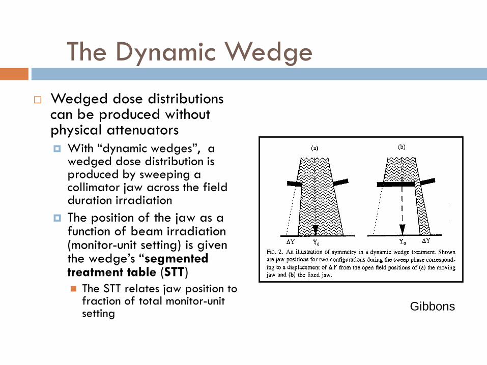
The Dynamic Wedge
Wedged dose distributions can be produced without physical attenuators With “dynamic wedges”, a
wedged dose distribution is produced by sweeping a collimator jaw across the field duration irradiation
The position of the jaw as a function of beam irradiation (monitor-unit setting) is given the wedge’s “segmented treatment table (STT)
The STT relates jaw position to fraction of total monitor-unit setting
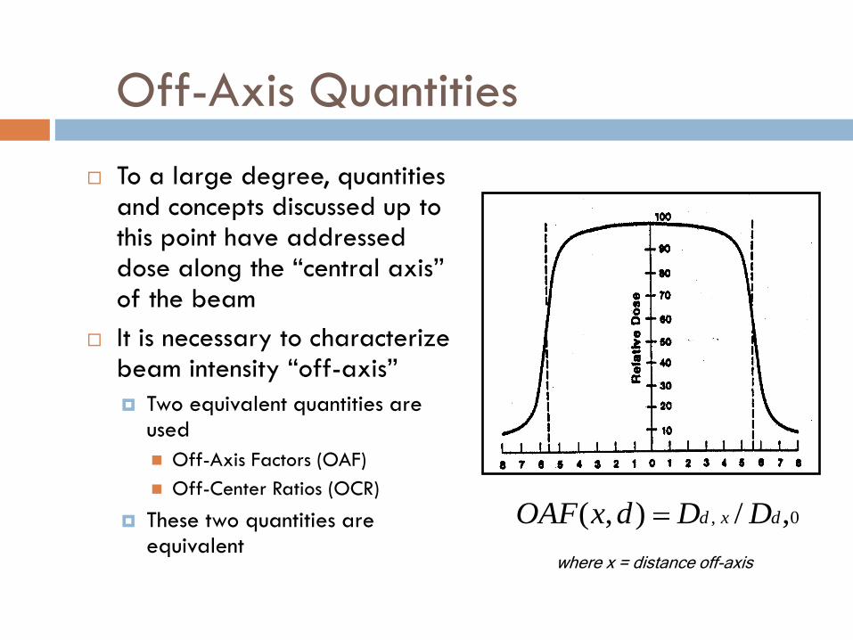
Off-Axis Quantities
To a large degree, quantities and concepts discussed up to this point have addressed dose along the “central axis” of the beam
It is necessary to characterize beam intensity “off-axis”
Two equivalent quantities are used
Off-Axis Factors (OAF)
Off-Center Ratios (OCR)
These two quantities are equivalent
0, ,/),( dxd DDdxOAF
where x = distance off-axis
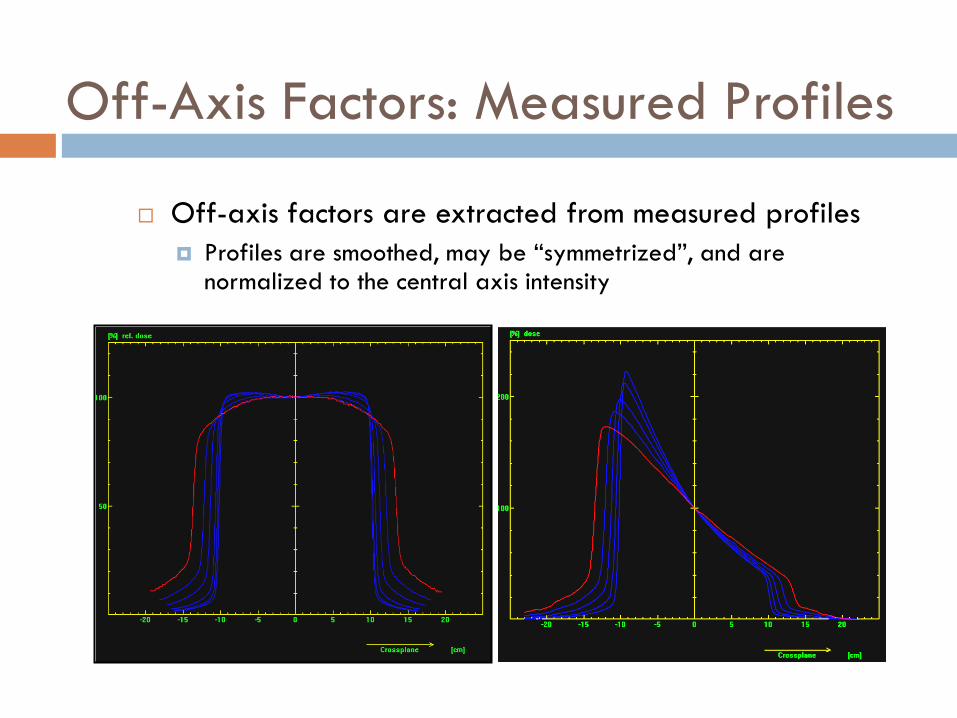
Off-Axis Factors: Measured Profiles
Off-axis factors are extracted from measured profiles
Profiles are smoothed, may be “symmetrized”, and are normalized to the central axis intensity
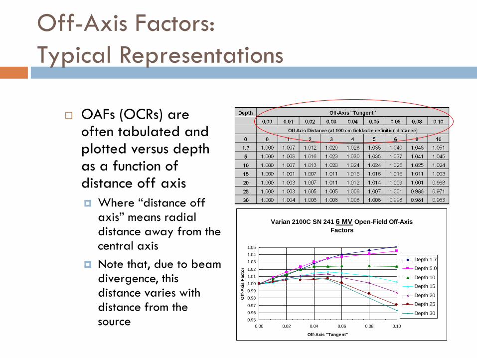
Off-Axis Factors:
Typical Representations
OAFs (OCRs) are often tabulated and plotted versus depth as a function of distance off axis
Where “distance off axis” means radial distance away from the central axis
Note that, due to beam divergence, this distance varies with distance from the source
Varian 2100C SN 241 6 MV Open-Field Off-Axis
Factors
0.95
0.96
0.97
0.98
0.99
1.00
1.01
1.02
1.03
1.04
1.05
0.00 0.02 0.04 0.06 0.08 0.10
Off-Axis "Tangent"
Off
-Axis
Facto
r
Depth 1.7
Depth 5.0
Depth 10
Depth 15
Depth 20
Depth 25
Depth 30

Off-Axis Wedge Corrections
Descriptions vary of off-axis intensity in wedged fields
Measured profiles contain both open-field off-axis intensity as well as differential wedge transmission
We have defined off-axis wedge corrections as corrections to the central axis wedge factor
Open-field off-axis intensity is divided out of the profile
The corrected profile is normalized to the central axis value
Dose Ratios: What have we learned
PDDs and TMRs
One has inverse square
and the other does not
Field Size
At what distance
Equivalent square
Scatter Factors
From accelerator head
From phantom (patient)
Almost halfway there …

Combine 1D Dosimetry Concepts
2D Dose Distributions
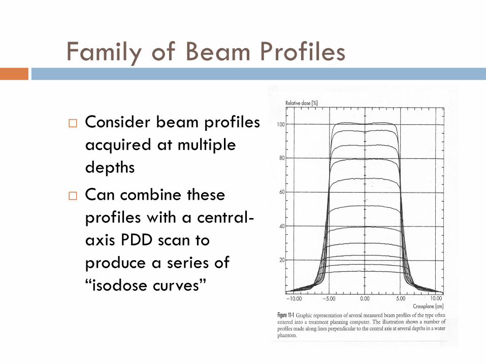
Family of Beam Profiles
Consider beam profiles
acquired at multiple
depths
Can combine these
profiles with a central-
axis PDD scan to
produce a series of
“isodose curves”

Isodose Curves
Isodose curves are “lines”
connecting equal intensities
or doses
Commonly normalized to dmax
along central axis
Characteristics
Flatness
Penumbra
Penetration
Depth of Dose Maximum

Wedged-field Isodose Distribution
Wedge angle defined
at
Depth of 80% (old
definition)
At 10 cm depth (new IEC
definition)
Distribution can be
normalized to dmax
central axis of wedged
field
Sometimes normalized to
open field

Isodose Curve Summation: Parallel
Opposed Fields
Hourglass
Shape

Parallel Opposed Fields
What are percent doses at midplane and at exit?

Two Pairs of Parallel Opposed
Fields
Using two pairs of
parallel opposed fields
at 90 degrees to each
other results in
peripheral doses on
the order of only 60-
70 percent of the
isocenter dose
The four-field box

Three Field Beam Arrangement
Increased avoidance of
critical structures can also be
achieved using a three field
technique
Three fields can introduce
challenges into daily setup,
however:
Table rail obstruction for beam
entry
Center spine obstruction for port
filming

Combinations of Wedged Fields

Penumbrae
Physical Penumbra
Is the region of the beam not irradiated by entire source
Accelerator source diameter is about 2 mm
Depends on source size, distance from the source to beam-definition device, and distance from source to measurement plane

-26 -24 -22 -20 -18 -16 -14 -12 -10 -8
0.1
0.2
0.3
0.4
0.5
0.6
0.7
0.8
0.9
1
Crossline position (mm)R
ela
tive D
ose
6MV3X3, d = 100 mm
CC01 unshifted
CC04 unshifted
Diode unshifted
Film
Penumbrae
Penumbrae of radiation
beams include scatter as
well as physical
characteristics
Common definition is distance
between 80% and 20%
isodose
Typical (corrected *)
penumbrae depend on
energy, and depth
3-6 mm 80%-20%
* corrected for detector
response
Schinkel, and others …

A “Physics Joke” …
Intermission
Take a brief break
Don’t go too far!
Stand up
Stretch
Is this OK … ??
“Dose Calculations”
is next

Calculation of linear accelerator monitor-unit
(MU) settings to deliver a prescribed dose
Dose Calculations
Problems

Our Sample Problem
A patient’s whole brain is to be treated.
The prescribed dose is 30 Gy total dose, 300 cGy
per fraction, 10 fractions, 5 fractions per week.
Radiation and technique are 6 MV x rays, parallel-
opposed right and left lateral fields; prescribed
dose is to isocenter.
Fields are 20x18, mlc-shaped
The patient set up for isocentric treatment at mid-
brain, lateral separation 16 cm

First rule of dose calcs …
Make a picture
Now … let’s reason this through ..

Output: From Relative Dose Ratios
to Absolute Dose
Standard calibration geometry
The geometry used to determine the dose output of the treatment
unit
Treatment units are calibrated such that their absolute dose is known at a
single point (the calibration point) in a predetermined (standard) geometry
Calibration geometries are SAD Calibration and SSD Calibration
Calibration Point Calibration Point
SAD
Calibration
SSD
Calibration

Introduction
Standard calibration point and geometry (SAD)
For linear accelerators in the Department of Radiation
Oncology, University of Maryland School of Medicine,
and commonly elsewhere, this point is located at dmax in a
water phantom, 100 cm SAD, along the central axis of an
open 10x10 field.
The unit is calibrated such that a dose equal to 1.0 cGy is
delivered to this point per 1 Monitor Unit (MU) setting

Introduction
Standard calibration geometry (SSD)
Other radiation oncology centers, UT M.D. Anderson
Cancer Center for example, use an SSD calibration
geometry
At these centers, this point is located at dmax in a water
phantom, 100 cm SSD, along the central axis of an
open standard field, most commonly the 10x10 field.
At this point (note – farther from the source), the unit is
calibrated such that 1 monitor unit (MU) is equal to 1.0
cGy
Introduction
Corrections to standard geometry
At depths other than dmax, distances other than the standard SAD
or SSD, and for field sizes other 10x10, and points off of the
central axis, corrections become necessary
Depth corrections are PPDs or TMRs,
Distance corrections are Inverse-Square corrections, and
Field-size corrections are Scatter Factors.
Corrections for points away from the central axis of the beam are
Off-Axis Factors
Corrections are also necessary to account for transmission through
beam attenuators such as wedges
These corrections are given in tabulated beam data where
relationships to the standard geometry have been established

Corrections to standard geometry: Summary
Depth corrections
Field-size corrections
Distance corrections
Off-axis corrections
Attenuation corrections
PDD, TAR, TMR
Output (scatter factors) ST SP SC
Inv. Sq. “SAD” or “SSD” Factors
OAFs
WFs, TFs, etc.
Formalism
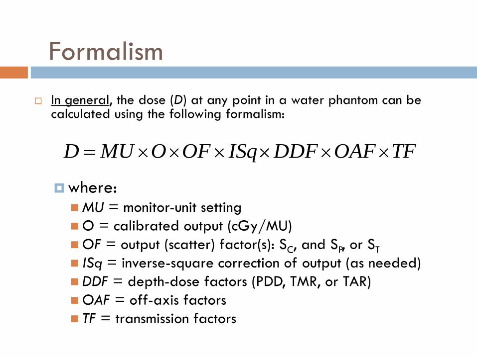
In general, the dose (D) at any point in a water phantom can be calculated using the following formalism:
where: MU = monitor-unit setting
O = calibrated output (cGy/MU)
OF = output (scatter) factor(s): SC, and SP, or ST
ISq = inverse-square correction of output (as needed)
DDF = depth-dose factors (PDD, TMR, or TAR)
OAF = off-axis factors
TF = transmission factors
TFOAFDDFISqOFOMUD
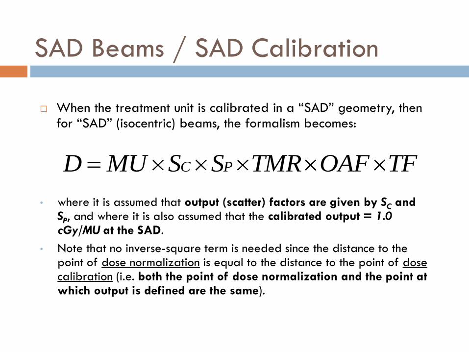
SAD Beams / SAD Calibration
When the treatment unit is calibrated in a “SAD” geometry, then for “SAD” (isocentric) beams, the formalism becomes:
• where it is assumed that output (scatter) factors are given by SC and SP, and where it is also assumed that the calibrated output = 1.0 cGy/MU at the SAD.
• Note that no inverse-square term is needed since the distance to the point of dose normalization is equal to the distance to the point of dose calibration (i.e. both the point of dose normalization and the point at which output is defined are the same).
TFOAFTMRSSMUD PC
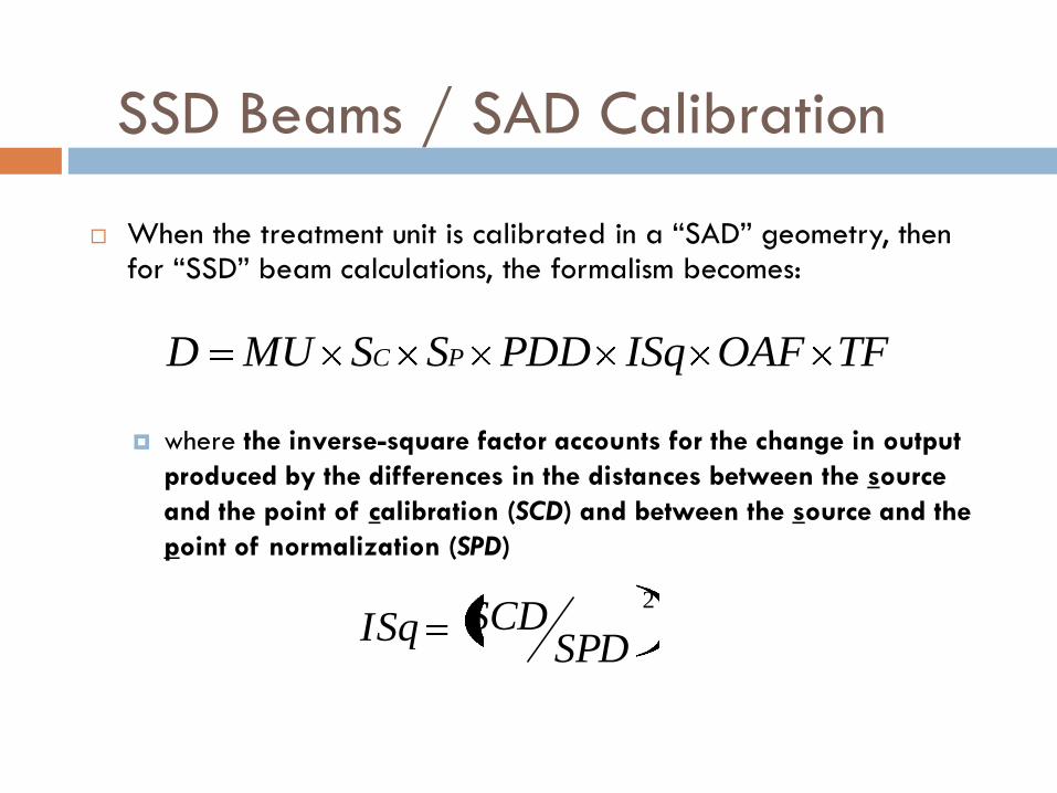
SSD Beams / SAD Calibration
When the treatment unit is calibrated in a “SAD” geometry, then for “SSD” beam calculations, the formalism becomes:
where the inverse-square factor accounts for the change in output
produced by the differences in the distances between the source
and the point of calibration (SCD) and between the source and the
point of normalization (SPD)
TFOAFISqPDDSSMUD PC
2
SPDSCDISq
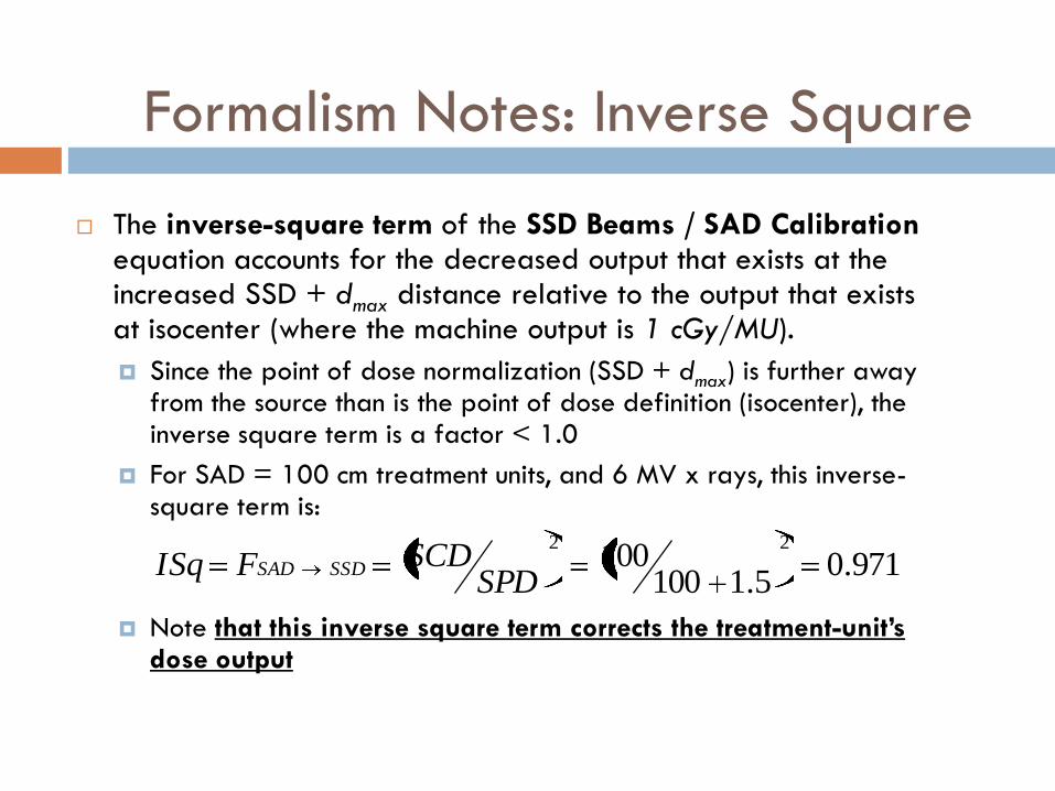
Formalism Notes: Inverse Square
The inverse-square term of the SSD Beams / SAD Calibration equation accounts for the decreased output that exists at the increased SSD + dmax distance relative to the output that exists at isocenter (where the machine output is 1 cGy/MU).
Since the point of dose normalization (SSD + dmax) is further away from the source than is the point of dose definition (isocenter), the inverse square term is a factor < 1.0
For SAD = 100 cm treatment units, and 6 MV x rays, this inverse-square term is:
Note that this inverse square term corrects the treatment-unit’s dose output
971.05.1100
10022
SPDSCDFISq SSDSAD

SSD Beams / SSD Calibration
When the treatment unit is calibrated in a “SSD” geometry, then for “SSD” beams, the formalism becomes:
Again, note that no inverse-square term is needed since the distance to the point of dose normalization (SSD + dmax) is equal to the distance to the point of dose calibration.
TFOAFPDDSSMUD PC

SAD Beams / SSD Calibration
When the treatment unit is calibrated in a “SSD” geometry, then
for “SAD” (isocentric) beams, the formalism becomes:
where again the inverse-square factor accounts for the change in
output produced by the differences in the distances between the
source and the point of calibration (SCD) and between the source
and the point of normalization (SPD):
The inverse-square correction in this case is a factor > 1.0, since
isocenter is closer to the source than is 100 SSD + dmax.
TFOAFTMRISqSSMUD PC
2
SPDSCDISq

Formalism Notes: Field Sizes
Field sizes, unless otherwise stated, represent collimator
settings
For most accelerators, field sizes are defined at 100 cm
(the distance from the source to isocenter)
For SSD beams, field sizes are defined at the surface (normally 100 cm
SSD)
For SAD beams, field sizes are defined at the depth of dose calculation
(normally 100 cm SAD)
For field sizes at distances other than 100 cm, field sizes
must be computed using triangulation:
100100, dSSDFSFS dSSD

Formalism Notes: Field Size Details
Scatter Factors, PDDs, TMRs
SC is a function of the collimator setting
SP is a function of the size of the field:
at the phantom surface for SSD beams
at the depth of calculation for SAD beams
PDDs are a function of:
field size at the phantom surface (SSD beams}
TMRs are a function of:
field size at depth (SAD beams)

Formalism Notes: Prescribed Dose
In general, one wishes to compute the MU setting necessary to
deliver a certain dose to a defined point.
This dose is “prescribed”, and
Its value must be known at the point of calculation.
When fields are combined to produce a prescribed dose at a
point, the doses from each field are computed from the
relative weights of each field.
Thus, if a dose DRx is prescribed through multiple fields i each having a
relative weight wti, then the dose Di from each field is:
i
iRxi
wtwtDD
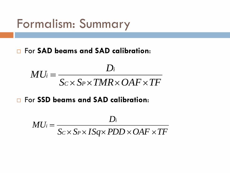
Formalism: Summary
For SAD beams and SAD calibration:
For SSD beams and SAD calibration:
TFOAFPDDISqSS
DMU
PC
ii
TFOAFTMRSS
DMU
PC
ii
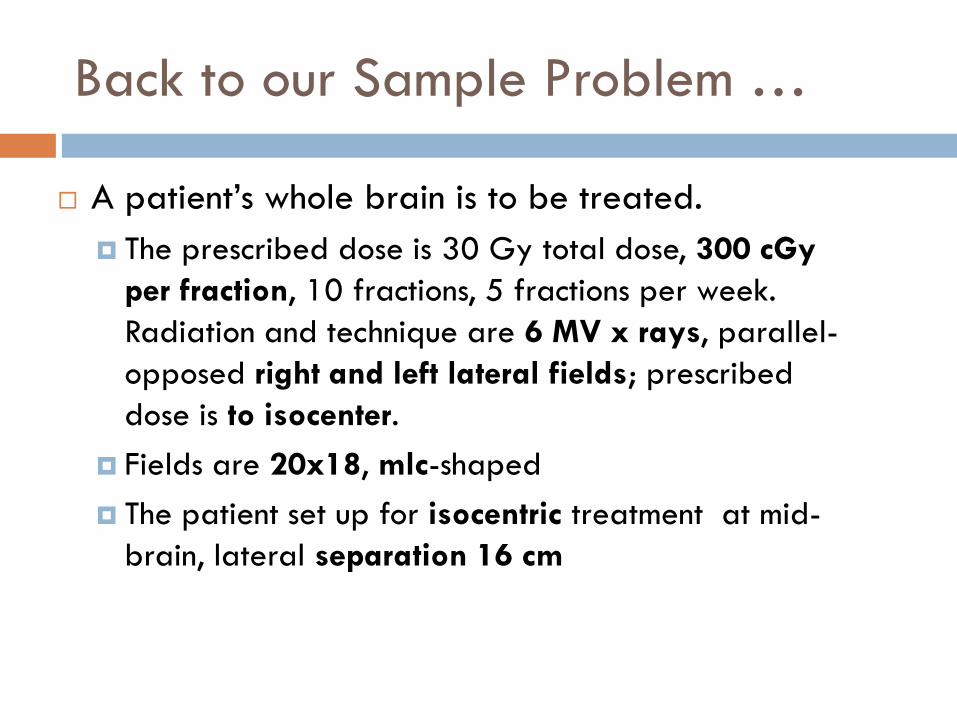
Back to our Sample Problem …
A patient’s whole brain is to be treated.
The prescribed dose is 30 Gy total dose, 300 cGy
per fraction, 10 fractions, 5 fractions per week.
Radiation and technique are 6 MV x rays, parallel-
opposed right and left lateral fields; prescribed
dose is to isocenter.
Fields are 20x18, mlc-shaped
The patient set up for isocentric treatment at mid-
brain, lateral separation 16 cm

Sample Problem
First compute equivalent squares
of the fields:
Then look up Output Factors and
TMRs
FS = 19 cm2 Depth = 8 cm
Substitute in:
And you’re done!
0.191820
182022WL
LWEqSq
TFOAFTMRSSDoseMU
PC
Assumes SAD Calibration

Thank You!
Clinical Dosimetry
Top Related