


Languages
Pages
Legal

Deep Network Interpolation
for Continuous Imagery Effect Transition
Xintao Wang1 Ke Yu1 Chao Dong2 Xiaoou Tang1 Chen Change Loy3
1CUHK - SenseTime Joint Lab, The Chinese University of Hong Kong2SIAT-SenseTime Joint Lab, Shenzhen Institutes of Advanced Technology, Chinese Academy of Sciences
3Nanyang Technological University, Singapore{wx016, yk017, xtang}@ie.cuhk.edu.hk [email protected] [email protected]
photo Van Gogh Ukiyo-e
deep DoF shallow DoF
MSE GAN
day night
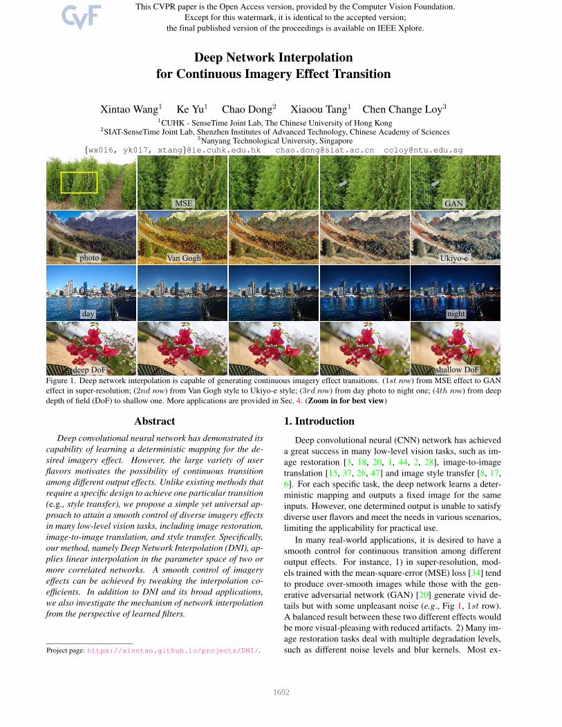
Figure 1. Deep network interpolation is capable of generating continuous imagery effect transitions. (1st row) from MSE effect to GAN
effect in super-resolution; (2nd row) from Van Gogh style to Ukiyo-e style; (3rd row) from day photo to night one; (4th row) from deep
depth of field (DoF) to shallow one. More applications are provided in Sec. 4. (Zoom in for best view)
Abstract
Deep convolutional neural network has demonstrated its
capability of learning a deterministic mapping for the de-
sired imagery effect. However, the large variety of user
flavors motivates the possibility of continuous transition
among different output effects. Unlike existing methods that
require a specific design to achieve one particular transition
(e.g., style transfer), we propose a simple yet universal ap-
proach to attain a smooth control of diverse imagery effects
in many low-level vision tasks, including image restoration,
image-to-image translation, and style transfer. Specifically,
our method, namely Deep Network Interpolation (DNI), ap-
plies linear interpolation in the parameter space of two or
more correlated networks. A smooth control of imagery
effects can be achieved by tweaking the interpolation co-
efficients. In addition to DNI and its broad applications,
we also investigate the mechanism of network interpolation
from the perspective of learned filters.
Project page: https://xinntao.github.io/projects/DNI/.
1. Introduction
Deep convolutional neural (CNN) network has achieved
a great success in many low-level vision tasks, such as im-
age restoration [3, 18, 20, 1, 44, 2, 28], image-to-image
translation [15, 37, 26, 47] and image style transfer [8, 17,
6]. For each specific task, the deep network learns a deter-
ministic mapping and outputs a fixed image for the same
inputs. However, one determined output is unable to satisfy
diverse user flavors and meet the needs in various scenarios,
limiting the applicability for practical use.
In many real-world applications, it is desired to have a
smooth control for continuous transition among different
output effects. For instance, 1) in super-resolution, mod-
els trained with the mean-square-error (MSE) loss [34] tend
to produce over-smooth images while those with the gen-
erative adversarial network (GAN) [20] generate vivid de-
tails but with some unpleasant noise (e.g., Fig 1, 1st row).
A balanced result between these two different effects would
be more visual-pleasing with reduced artifacts. 2) Many im-
age restoration tasks deal with multiple degradation levels,
such as different noise levels and blur kernels. Most ex-
1692

isting methods can only handle limited degradation levels.
It is costly to train lots of models for continuous degrada-
tion levels in practice. Thus, a model with the flexibility of
adjusting the restoration strength would expand the appli-
cation coverage. 3) In artistic manipulation like image-to-
image translation and image style transfer, different users
have different aesthetic flavors. Achieving a smooth control
for diverse effects with a sliding bar are appealing in these
applications.
Several approaches have been proposed to improve the
CNN’s flexibility for producing continuous transitions in
different tasks. Take image style transfer as an example,
adaptive scaling and shifting parameters are used in instance
normalization layers [6, 12] for modeling different styles.
Interpolating these normalization parameters for different
styles produces the combination of various artistic styles. In
order to further control the stroke size in the stylized results,
a carefully-designed pyramid structure consisting of several
stroke branches are proposed [16]. Though these methods
are able to realize continuous transition, there are several
drawbacks: 1) These careful designs are problem-specific
solutions, lacking the generalizability to other tasks. 2)
Modifications to existing networks are needed, thus com-
plicate the training process. 3) There is still no effective
and general way to solve the smooth control in tasks like
balancing MSE and GAN effects in super-resolution.
In this paper, we address these drawbacks by introduc-
ing a more general, simple but effective approach, known
as Deep Network Interpolation (DNI). Continuous imagery
effect transition is achieved via linear interpolation in the
parameter space of existing trained networks. Specifically,
provided with a model for a particular effect A, we fine-tune
it to realize another relevant effect B. DNI applies linear
interpolation for all the corresponding parameters of these
two deep networks. Various interpolated models can then be
derived by a controllable interpolation coefficient. Perform-
ing feed-forward operations on these interpolated models
using the same input allows us to outputs with a continuous
transition between the different effects A and B.
Despite its simplicity, the proposed DNI can be applied
to many low-level vision tasks. Some examples are pre-
sented in Fig 1. Extensive applications showcased in Sec. 4
demonstrate that deep network interpolation is generic for
many problems. DNI also enjoys the following merits. 1)
The transition effect is smooth without abrupt changes dur-
ing interpolation. The transition can be easily controlled by
an interpolation coefficient. 2) The linear interpolation op-
eration is simple. No network training is needed for each
transition and the computation for DNI is negligible. 3)
DNI is compatible with popular network structures, such
as VGG [31], ResNet [10] and DenseNet [11].
Our main contribution in this work is the novel notion
of interpolation in parameter space, and its application in
low-level vision tasks. We demonstrate that interpolation in
the parameter space could achieve much better results than
mere pixel interpolation. We further contribute a system-
atic study that investigates the mechanism and effectiveness
of parameter interpolation through carefully analyzing the
filters learned.
2. Related Work
Image Restoration. CNN-based approaches have led to a
series of breakthroughs for several image restoration tasks
including super-resolution [3, 18, 25, 19, 33, 20, 43], de-
noising [1, 44], de-blocking [40, 7] and deblurring [42, 32,
28]. While most of the previous works focus on address-
ing one type of distortion without the flexibility of adjusting
the restoration strength, there are several pioneering works
aiming to handle various practical scenarios with control-
lable “hyper-parameters”. Zhang et al. [45] adopt CNN
denoisers to solve image restoration tasks by manually se-
lecting the hyper-parameters in a model-based optimiza-
tion framework. However, a bank of discriminative CNN
denoisers are required and the hyper-parameter selection
in optimization is not a trivial task [4]. SRMD [46] pro-
poses an effective super-resolution network handling mul-
tiple degradations by taking an degradation map as extra
inputs. However, the employed dimensionality stretching
strategy is problem-specific, lacking the generalizability to
other tasks.
Image Style Transfer. Gatys et al. [8] propose the neural
style transfer algorithm for artistic stylization. A number of
methods are developed to further improve its performance
and speed [35, 17, 21]. In order to model various/arbitrary
styles in one model, several techniques are developed, in-
cluding conditional instance normalization [6], adaptive in-
stance normalization [12, 9] and whitening and coloring
transforms [23]. These carefully-designed approaches are
also able to achieve user control. For example, interpolating
the normalization parameters of different styles produces
the combination of various artistic styles. The balance of
content and style can be realized by adjusting the weights
of their corresponding features during mixing. In order to
control the stroke size, a specially designed pyramid struc-
ture consisting of several stroke branches are further pro-
posed [16]. In these studies, different controllable factors
require specific structures and strategies.
Image-to-image Translation. Image-to-image transla-
tion [15, 37, 26, 47, 13] aims at learning to translate an
image from one domain to another. For instance, from
landscape photos to Monet paintings, and from smartphone
snaps to professional DSLR photographs. These methods
can only transfer an input image to a specific target mani-
fold and they are unable to produce continuous translations.
The controllable methods proposed in image restoration and
image style transfer are problem-specific and cannot be di-
1693
rectly applied to the different image-to-image translation
task. On the contrary, the proposed DNI is capable of deal-
ing with all these problems in a general way, regardless of
the specific characteristics of each task.
Interpolation. Instead of performing parameter interpola-
tion, one can also interpolate in the pixel space or feature
space. However, it is well known that interpolating images
pixel by pixel introduces ghosting artifacts since natural im-
ages lie on a non-linear manifold [41]. Upchurch et al. [36]
propose a linear interpolation of pre-trained deep convo-
lutional features to achieve image content changes. This
method requires an optimization process when inverting the
features back to the pixel space. Moreover, it is mainly de-
signed for transferring facial attributes and not suitable for
generating continuous transition effects for low-level vision
tasks. More broadly, several CNN operations in the in-
put and feature space have been proposed to increase the
model’s flexibility. Concatenating extra conditions to in-
puts [46] or to middle features [22] alters the network be-
havior in various scenes. Modulating features with an affine
transformation [29, 5, 38] is able to effectively incorporate
other information. Different from these works, we make
an attempt to investigate the manipulation in the parameter
space. A very preliminary study for network interpolation
is presented by ESRGAN [39], focusing to enhance compe-
tition results. DNI provides more comprehensive investiga-
tions and extends to more applications.
3. Methodology
3.1. Deep Network Interpolation
Many low-level vision tasks, e.g., image restoration,
image style transfer, and image-to-image translation, aim
at mapping a corrupted image or conditioned image x to
the desired one y. Deep convolutional neural networks
are applied to directly learn this mapping function Gθ
parametrized by θ as y = Gθ(x).
Consider two networks GA and GB with the same struc-
ture, achieving different effects A and B, respectively. The
networks consist of common operations such as convolu-
tion, up/down-sampling and non-linear activation. The pa-
rameters in CNNs are mainly the weights of convolutional
layers, called filters, filtering the input image or the prece-
dent features. We assume that their parameters θA and θBhave a “strong correlation” with each other, i.e., the filter or-
ders and filter patterns in the same position of GA and GB
are similar. This could be realized by some constraints like
fine-tuning, as will be analyzed in Sec. 3.2. This assumption
provides the possibility for meaningful interpolation.
Our aim is to achieve a continuous transition between the
effects A and B. We do so by the proposed Deep Network
Interpolation (DNI). DNI interpolates all the corresponding
parameters of these two models to derive a new interpolated
model Ginterp, whose parameters are:
θinterp = α θA + (1− α) θB , (1)
where α ∈ [0, 1] is the interpolation coefficient. Indeed,
it is a linear interpolation of the two parameter vectors θAand θB . The interpolation coefficient α controls a balance
of the effect A and B. By smoothly sliding α, we achieve
continuous transition effects without abrupt changes.
Generally, DNI can be extended for N models, denoted
by G1, G2, ..., GN , whose parameters have a “close corre-
lation” with each other. The DNI is then formulated as:
θinterp = α1θ1 + α2θ2 + ...+ αNθN , (2)
where αi satisfy αi ≥ 0 and α1 + α2 + · · · + αN = 1.
In other words, it is a convex combination of the param-
eter vectors θ1, θ2, ..., θN . By adjusting (α1, α2, ..., αN ), a
rich and diverse effects with continuous transitions could be
realized.
The interpolation is performed on all the layers with pa-
rameters in the networks, including convolutional layers
and normalization layers. Convolutional layers have two
parameters, namely weights (filters) and biases. The biases
are added to the results after filtering operation with filters.
Apart from the weights, DNI also operates on the biases,
since the added biases influence the successive non-linear
activation.
Batch normalization (BN) layers [14] have two kinds of
parameters. 1) The statistics running mean and running var
track the mean and variance of the whole dataset during
training and are then used for normalization during eval-
uation. 2) the learned parameters γ and β are for a fur-
ther affine transformation. During inference, all these four
parameters actually could be absorbed into the precedent
or successive convolutional layers. Thus, DNI also per-
forms on normalization parameters. Instance normalization
(IN) has a similar behavior as BN, except that IN uses in-
stance statistics computed from input data in both training
and evaluation. We take the same action as that for BN.
In practice, the interpolation is performed on not only the
weights but also the biases and further normalization lay-
ers. We believe a better interpolation scheme considering
the property of different kinds of parameters is worthy of
exploiting.
It is worth noticing that the choice of the network struc-
ture for DNI is flexible, as long as the structures of mod-
els to be interpolated are kept the same. Our experiments
on different architectures show that DNI is compatible with
popular network structures such as VGG [31], ResNet [10]
and DenseNet [11]. We also note that the computation of
DNI is negligible. The computation is only proportional to
the number of parameters.
1694
43 575 16 1915 503
a b c
ed f
filterindex
N20
run 1
N20run 2
N60fine-tuned
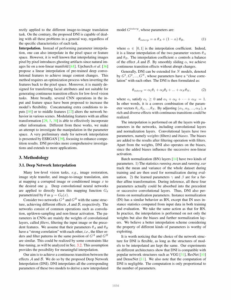
Figure 2. Filter correlations. The first two rows are the filters of
different runs (both from scratch) for the denoising (N20) task.
The filter orders and filter patterns in the same position are differ-
ent. The fine-tuned model (N60) (3rd row) has a “strong correla-
tion” to the pre-trained one (1st row).
3.2. Understanding Network Interpolation
We attempt to gain more understanding on network in-
terpolation from some empirical studies. From our experi-
ments, we observe that: 1) Fine-tuning facilitates high cor-
relation between parameters of different networks, provid-
ing the possibility for meaningful interpolation. 2) Fine-
tuned filters for a series of related tasks present continu-
ous changes. 3) Our analyses show that interpolated filters
could fit the actual learned filters well. Note that our anal-
yses mainly focus on filters since most of the parameters in
CNNs are in the form of filters.
We present our main observations with a representative
denoising task and focus on increasing noise levels with
N20, N30, N40, N50, and N60, where N20 denotes the
Gaussian noise with zero mean and variance 20. In order
to better visualize and analyze the filters, we adopt a three-
layer network similar to SRCNN [3], where the first and last
convolutional layers have 9×9 filter size. Following the no-
tion of [3], the first and last layer layers can be viewed as a
feature extraction and reconstruction layer, respectively.
Fine-tuning for inter-network correlation. Even for the
same task like denoising with the N20 level, if we simply
train two models from scratch, the filter orders among chan-
nels and filter patterns in the corresponding positions could
be very different (Fig. 2). However, a core representation
is shared between these two networks [24]. For instance, in
Fig. 2, filer c is identical to filter f ; filter a and filter e have a
similar pattern but with different colors; filter b is a inverted
and rotated counterpart of filter d.
Fine-tuning, however, can help to maintain the filters’s
order and pattern. To show this, we fine-tune a pre-trained
network (N20) to a relevant task (N60). It is observed that
the filter orders and filter patterns are maintained (Fig. 2).
The “high correlation” between the parameters of these two
networks provides the possibility for meaningful interpo-
lation. We note that besides fine-tuning, other constraints
such as joint training with regularization may also achieve
such inter-network correlation.
Learned filters for related tasks exhibit continuous
changes. When we fine-tune several models for relevant
N20 N30 N40 N50 N60
learned
interp
N20 N30 N40 N50 N60feature extraction layer reconstruction layer
0.75
0.8
0.85
0.9
0.95
1
learned
interp
learned
interp
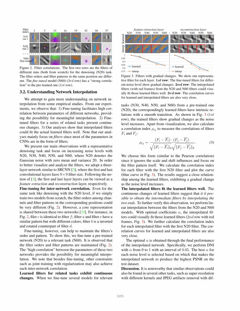
Figure 3. Filters with gradual changes. We show one representa-
tive filter for each layer. 1st row: The fine-tuned filters for differ-
ent noise level show gradual changes. 2nd row: The interpolated
filters (with red frames) from the N20 and N60 filters could visu-
ally fit those learned filters well. 3rd row: The correlation curves
for learned and interpolated filters are also very close.
tasks (N30, N40, N50, and N60) from a pre-trained one
(N20), the correspondingly learned filters have intrinsic re-
lations with a smooth transition. As shown in Fig. 3 (1strow), the trained filters show gradual changes as the noise
level increases. Apart from visualization, we also calculate
a correlation index ρij to measure the correlations of filters
Fi and Fj :
ρij =(Fi − Fi) · (Fj − Fj)
√
‖Fi − Fi‖2
√
‖Fj − Fj‖2
. (3)
We choose this form (similar to the Pearson correlation)
since it ignores the scale and shift influences and focus on
the filter pattern itself. We calculate the correlation index
for each filter with the first N20 filter and plot the curve
(blue curve in Fig. 3). The results suggest a close relation-
ship among the learned filters, exhibiting a gradual change
as the noise level increases.
The interpolated filters fit the learned filters well. The
continuous changes of learned filters suggest that it it pos-
sible to obtain the intermediate filters by interpolating the
two ends. To further verify this observation, we perform lin-
ear interpolation between the filters from the N20 and N60
models. With optimal coefficients α, the interpolated fil-
ters could visually fit those learned filters (2nd row with red
frames, Fig. 3). We further calculate the correlation index
for each interpolated filter with the first N20 filter. The cor-
relation curves for learned and interpolated filters are also
very close.
The optimal α is obtained through the final performance
of the interpolated network. Specifically, we perform DNI
with α from 0 to 1 with an interval of 0.05. The best α for
each noise level is selected based on which that makes the
interpolated network to produce the highest PSNR on the
test dataset.
Discussion. It is noteworthy that similar observations could
also be found in several other tasks, such as super-resolution
with different kernels and JPEG artifacts removal with dif-
1695

ferent compression levels. We provide the details in the sup-
plementary material.
The analysis above is by no means complete, but it gives
a preliminary explanation behind the DNI from the filter
perspective. As the network goes deeper, the non-linearity
increases and the network behaviors become more compli-
cated. However, we still observe a similar phenomenon
for deeper networks. Since filter visualization is difficult
in deep networks, which typically designed with a stack of
convolutional layers of 3 × 3 kernels, we adopt the corre-
lation index (Eq. 3) to analyze the filter correlations among
models for a series of noise levels. We employ DnCNN [44]
with 17 layers and analyze the 5th (the front) and 12th (the
back) convolutional layers. In Fig. 4, the correlation curves
show the median of correlation indexes w.r.t. the first N20
model and the correlation distribution are also plotted. Be-
sides the high correlation among these models, we can also
observe gradual changes as the noise level increases. Fur-
thermore, the front and the back convolution layers present
a similar transition trend, even their distributions highly co-
incide.
1.00
0.95
0.90
0.85
N20 N30 N40 N50 N60
12th conv
5th conv
Noise level
co
rrela
tio
n i
nd
ex
Figure 4. Filter correlation for deeper denoising networks. We
show a front (5th) and a back (12th) layer. The curves present
the median of correlation indexes and the correlation distribution
are also plotted. Note that the two distributions highly coincide.
Zoom in for subtle differences.
4. Applications
We experimentally show that the proposed DNI can
be applied to extensive low-level vision tasks, e.g., image
restoration (Sec. 4.1), image-to-image translation (Sec. 4.2)
and image style transfer (Sec. 4.3). Another example
of smooth transitions on face attributes are presented in
Sec. 4.4, indicating its potential for semantic changes. Due
to space limitations, more examples and analyses are pro-
vided in the supplementary material and the project page1.
4.1. Image Restoration
Balance MSE and GAN effects in super-resolution. The
aim of super-resolution is to estimate a high-resolution im-
1https://xinntao.github.io/projects/DNI
age from its low-resolution counterpart. A super-resolution
model trained with MSE loss [34] tends to produce over-
smooth images. We fine-tune it with GAN loss and percep-
tual loss [20], obtaining results with vivid details but always
together with unpleasant artifacts (e.g., the eaves and water
waves in Fig. 5). We use dense blocks [11, 39] in the net-
work architecture and the MATLAB bicubic kernel with a
scaling factor of 4 is adopted as the down-sampling kernel.
As presented in Fig. 5, DNI is able to smoothly alter
the outputs from the MSE effect to the GAN effect. With
appropriate interpolation coefficient, it produces visually-
pleasing results with largely reduced artifacts while main-
taining the textures. We also compare it with pixel interpo-
lation, i.e., interpolating the output images pixel by pixel.
However, the pixel interpolation is incapable of separating
the artifacts and details. Taking the water waves for exam-
ple (Fig. 5), the water wave texture and artifacts simulta-
neously appear and enhance during the transition. Instead,
DNI first enhances the vivid water waves without artifacts
and then finer textures and undesirable noise appears suc-
cessively. The effective separation helps to remove the dis-
pleasing artifacts while keeping the favorable textures, su-
perior to the pixel interpolation. This property could also be
observed in the transition of animal fur in Fig. 5, where the
main structure of fur first appears followed by finer struc-
tures and subtle textures.
One can also obtain several models for different mixture
effects, by tuning the weights of MSE loss and GAN loss
during training. However, this approach requires tuning on
the loss weights and training many networks for various bal-
ances, and thus it is too costly to achieve continuous control.
Adjust denoising strength. The goal of denoising is to
recover a clean image from a noisy observation. In order
to satisfy various user demands, most popular image edit-
ing softwares (e.g., Photoshop) have controllable options
for each tool. For example, the noise reduction tool comes
with sliding bars for controlling the denoising strength and
the percentage of preserving or sharpening details.
We show an example to illustrate the importance of ad-
justable denoising strength. We are provided with a de-
noising model specialized in addressing a specific Gaussian
noise level N40. We use DnCNN [44] as our implementa-
tion. As shown in Fig. 6, however, the determined outputs
(with yellow frames) are not satisfactory due to the differ-
ent imagery contents. In particular, the denoising strength
for the grass is too strong, producing over-smooth results,
while in the smooth sky region, it requires a larger strength
to remove the undesired artifacts.
Existing deep-learning based approaches fail to meet this
user requirements since they are trained to generate deter-
ministic results without the flexibility to control the denois-
ing strength. On the contrary, our proposed DNI is able to
achieve adjustable denoising strength by simply tweaking
1696

compare with
pixel interpolation
MSE effect GAN effect
Figure 5. Balancing the MSE and GAN effects with DNI in super-resolution. The MSE effect is over-smooth while the GAN effect is
always accompanied with unpleasant artifacts (e.g., the eaves and water waves). DNI allows smooth transition from one effect to the other
and produces visually-pleasing results with largely reduced artifacts while maintaining the textures. In contrast, the pixel interpolation
strategy fails to separate the artifacts and textures. (Zoom in for best view)
grass
DnCNN baseweaker denosing strength stronger denosing strength
corrupted
sky
Figure 6. Adjustable denoising strength with DNI. One model without adjustment (with yellow frames) is unable to balance the noise
removal and detail preservation. For the grass, a weaker denoising strength could preserve more textures while for the sky, the stronger
denoising strength could obtain an artifact-free result, improving the visual quality (with red frames). (Zoom in for best view)
the interpolation coefficient α of different denoising models
for N20, N40 and N60. For the grass, a weaker denoising
strength could preserve more details while in the sky region,
the stronger denoising strength could obtain an artifact-free
result (red frames in Fig. 6). This example demonstrates the
flexibility of DNI to customize restoration results based on
the task at hand and the specific user preference.
4.2. Imagetoimage Translation
Image-to-image translation aims at learning to translate
an image from one domain to another. Most existing ap-
proaches [15, 37, 26, 47] can only transfer one input image
to several discrete outputs, lacking continuous translation
for diverse user flavors. For example, one model may be
able to mimic the style of Van Gogh or Cezanne, but trans-
lating a landscape photo into a mixed style of these two
painters is still challenging.
The desired continuous transition between two painters’
styles can be easily realized by DNI. The popular Cycle-
GAN [47] is used as our implementation. We first train
a network capturing characteristics of Van Gogh, and then
fine-tune it to produce paintings of Cezanne’s style. DNI is
capable of generating various mixtures of these two styles
given a landscape photo, by adjusting the interpolation co-
efficient. Fig. 7a presents a smooth transition from Van
Gogh’s style to Cezanne’s style both in the palette and brush
strokes. We note that DNI can be further employed to mix
styles of more than two painters using Eq. 2. Results are
provided in the supplementary material.
In addition to the translation between painting styles of
a whole image, DNI can also achieve smooth and natural
translation for a particular image region. Fig. 7b shows
an example of photo enhancement to generate photos with
shallower depth of field (DoF). We train one model to gen-
erate flower photos with shallow DoF and then fine-tune it
with identity mapping. DNI is then able to produce con-
1697

Van Gogh Cézannephoto(a) Photos to paintings. DNI produces a smooth transition from Van Gogh’s style to Cezanne’s style both in the palette and brush strokes.
DNI (ours)
pixel interpolation
depth of field shallowdeep(b) Smooth transition on depth of field with DNI. However, pixel interpolation generates ghosting artifacts. (Zoom in for best view)
day night(c) Day photos to night ones. As the night approaches, it is getting darker and the lights are gradually lit up, reflected on the water.
Figure 7. Several applications for image-to-image translation. (Zoom in for best view)
tinuous transitions of DoF by interpolating these two mod-
els. We also compare DNI with pixel interpolation, where
the results look unnatural due to the ghosting artifacts, e.g.,
translucent details appearing at the edge of blurry leaves.
DNI can be further applied to achieve continuous im-
agery translations in other dimensions such as light changes,
i.e., transforming the day photos to night ones. Only trained
with day and night photos, DNI is capable of generating
a series of images, simulating the coming of nights. In
Fig. 7c, as the night approaches, it is getting darker and the
lights are gradually lit up, reflected on the water.
4.3. Style Transfer
There are several controllable factors when transferring
the styles of one or many pieces of art to an input image,
e.g., style mixture, stroke adjustment and the balance of
content and style. Some existing approaches design spe-
cific structures to achieve a continuous control of these fac-
tors [16]. On the contrary, DNI offers a general way to at-
tain the same goals without specific solutions. As shown in
Fig. 8, DNI is capable of generating smooth transitions be-
tween different styles, from large to small strokes, together
with balancing the content and style. Furthermore, DNI can
be applied among multiple models to achieve a continuous
control of various factors simultaneously. For instance, the
stroke and style can be adjusted at the same time based on
user flavors, as shown in Fig. 8.
Another branch of existing methods achieves a combina-
tion of various artistic styles by interpolating the parameters
of instance normalization (IN) [6, 12]. These approaches
can be viewed as a special case of DNI, where only IN
parameters are fine-tuned and interpolated. To clarify the
difference between DNI and IN interpolation, we conduct
experiments with 3 settings: 1) fine-tune IN; 2) fine-tune
convolutional layers and 3) fine-tune both IN and convo-
lutional layers. Specifically, as shown in Fig. 9, we try a
challenging task to fine-tune the model from generating im-
ages with mosaic styles to the one with fire styles, where
the two styles look very different in both color and texture.
It is observed that fine-tuning only IN is effective in color
transformation, however, it is unable to transfer the fire tex-
ture effectively compared with the other two settings. This
observation suggests that convolutional layers also play an
important role in style modeling, especially for the textures,
since IN parameters may not be effective for capturing spa-
tial information. However, we do not claim that DNI is con-
sistently better than IN interpolation, since IN is also effec-
tive in most cases. A more thorough study is left for future
work.
4.4. Semantic Transition
Apart from low-level vision tasks, we show that DNI can
also be applied for smooth transitions on face attributes,
suggesting its potential for semantic adjustment. We first
1698

style
stro
ke
balance of content and styleFigure 8. In image style transfer, without specific structures and strategies, DNI is capable of generating smooth transitions between
different styles, from large strokes to small strokes, together with balancing the content and style. (Zoom in for best view)
only fine-tune IN only fine-tune conv fine-tune conv and IN
Figure 9. Fine-tuning only IN is effective in color transformation,
however, it is unable to transfer the fire texture effectively.
male female
young old
Figure 10. Smooth transitions on face attributes with DNI.
train a DCGAN model [30] using the CelebA [27] dataset
with one attribute (e.g., young or male). After that, we fine-
tune it to generate faces with another attribute (e.g., old or
female). DNI is then able to produce a series of faces with
smoothly transformed attributes by interpolating these mod-
els (Fig. 10). Although neither of the interpolated models
observes any data with middle attributes, the faces in mid-
dle states has an intermediate attribute and looks natural.
4.5. Limitations
We have shown that DNI offers a simple yet general ap-
proach for transition manipulation. However, DNI also has
limitations - 1) it needs fine-tuning or jointly training, oth-
erwise the interpolated model is meaningless; 2) if the two
(or several) tasks have little relation (i.e., DNNs trained for
different tasks), the interpolated model could not produce
meaningful results. We examine the correlation indexes of
successfully interpolated models, which are in [0.689, 1).
But for those failure cases, the correlation indexes are ex-
tremely small (<0.1). Future work will investigate how to
quantify the network ‘distance’ and task ‘distance’ for DNI.
5. Conclusion
In this paper, we propose a novel notion of interpola-
tion in the parameter space, i.e., applying linear interpola-
tion among the corresponding parameters of multiple corre-
lated networks. The imagery effects change smoothly while
adjusting the interpolation coefficients. With extensive ex-
periments on super-resolution, denoising, image-to-image
translation and style transfer, we demonstrate that the pro-
posed method is applicable for a wide range of low-level
vision tasks despite its simplicity. Compared with existing
methods that achieve continuous transition by task-specific
designs, our method is easy to generalize with negligible
computational overhead. Future work will investigate the
effects of network interpolation on high-level tasks.
Acknowledgement. This work is supported by Sense-
Time Group Limited, Joint Lab of CAS-HK, the Gen-
eral Research Fund sponsored by the Research Grants
Council of the Hong Kong SAR (CUHK 14241716,
14224316. 14209217), and Singapore MOE AcRF Tier 1
(M4012082.020).
1699

References
[1] Harold C Burger, Christian J Schuler, and Stefan Harmeling.
Image denoising: Can plain neural networks compete with
BM3D? In CVPR, 2012. 1, 2
[2] Chao Dong, Yubin Deng, Chen Change Loy, and Xiaoou
Tang. Compression artifacts reduction by a deep convolu-
tional network. In ICCV, 2015. 1
[3] Chao Dong, Chen Change Loy, Kaiming He, and Xiaoou
Tang. Learning a deep convolutional network for image
super-resolution. In ECCV, 2014. 1, 2, 4
[4] Weisheng Dong, Lei Zhang, Guangming Shi, and Xin
Li. Nonlocally centralized sparse representation for image
restoration. TIP, 22(4):1620–1630, 2013. 2
[5] Vincent Dumoulin, Ethan Perez, Nathan Schucher, Flo-
rian Strub, Harm de Vries, Aaron Courville, and Yoshua
Bengio. Feature-wise transformations. Distill, 2018.
https://distill.pub/2018/feature-wise-transformations. 3
[6] Vincent Dumoulin, Jonathon Shlens, Manjunath Kudlur,
Arash Behboodi, Filip Lemic, Adam Wolisz, Marco Moli-
naro, Christoph Hirche, Masahito Hayashi, Emilio Bagan,
et al. A learned representation for artistic style. In ICLR,
2016. 1, 2, 7
[7] Leonardo Galteri, Lorenzo Seidenari, Marco Bertini, and Al-
berto Del Bimbo. Deep generative adversarial compression
artifact removal. In ICCV, 2017. 2
[8] Leon A Gatys, Alexander S Ecker, and Matthias Bethge. Im-
age style transfer using convolutional neural networks. In
CVPR, 2016. 1, 2
[9] Golnaz Ghiasi, Honglak Lee, Manjunath Kudlur, Vincent
Dumoulin, and Jonathon Shlens. Exploring the structure of
a real-time, arbitrary neural artistic stylization network. In
BMVC, 2017. 2
[10] Kaiming He, Xiangyu Zhang, Shaoqing Ren, and Jian Sun.
Deep residual learning for image recognition. In CVPR,
2016. 2, 3
[11] Gao Huang, Zhuang Liu, Kilian Q Weinberger, and Laurens
van der Maaten. Densely connected convolutional networks.
In CVPR, 2017. 2, 3, 5
[12] Xun Huang and Serge Belongie. Arbitrary style transfer in
real-time with adaptive instance normalization. In ICCV,
2017. 2, 7
[13] Xun Huang, Ming-Yu Liu, Serge Belongie, and Jan Kautz.
Multimodal unsupervised image-to-image translation. In
ECCV, 2018. 2
[14] Sergey Ioffe and Christian Szegedy. Batch normalization:
Accelerating deep network training by reducing internal co-
variate shift. In ICMR, 2015. 3
[15] Phillip Isola, Jun-Yan Zhu, Tinghui Zhou, and Alexei A
Efros. Image-to-image translation with conditional adver-
sarial networks. In CVPR, 2017. 1, 2, 6
[16] Yongcheng Jing, Yang Liu, Yezhou Yang, Zunlei Feng,
Yizhou Yu, Dacheng Tao, and Mingli Song. Stroke con-
trollable fast style transfer with adaptive receptive fields. In
ECCV, 2018. 2, 7
[17] Justin Johnson, Alexandre Alahi, and Li Fei-Fei. Perceptual
losses for real-time style transfer and super-resolution. In
ECCV, 2016. 1, 2
[18] Jiwon Kim, Jung Kwon Lee, and Kyoung Mu Lee. Accurate
image super-resolution using very deep convolutional net-
works. In CVPR, 2016. 1, 2
[19] Wei-Sheng Lai, Jia-Bin Huang, Narendra Ahuja, and Ming-
Hsuan Yang. Deep laplacian pyramid networks for fast and
accurate super-resolution. In CVPR, 2017. 2
[20] Christian Ledig, Lucas Theis, Ferenc Huszar, Jose Caballero,
Andrew Cunningham, Alejandro Acosta, Andrew Aitken,
Alykhan Tejani, Johannes Totz, Zehan Wang, et al. Photo-
realistic single image super-resolution using a generative ad-
versarial network. In CVPR, 2017. 1, 2, 5
[21] Chuan Li and Michael Wand. Combining markov random
fields and convolutional neural networks for image synthesis.
In CVPR, 2016. 2
[22] Yijun Li, Chen Fang, Jimei Yang, Zhaowen Wang, Xin Lu,
and Ming-Hsuan Yang. Diversified texture synthesis with
feed-forward networks. In CVPR, 2017. 3
[23] Yijun Li, Chen Fang, Jimei Yang, Zhaowen Wang, Xin Lu,
and Ming-Hsuan Yang. Universal style transfer via feature
transforms. In NIPS, 2017. 2
[24] Yixuan Li, Jason Yosinski, Jeff Clune, Hod Lipson, and
John E Hopcroft. Convergent learning: Do different neu-
ral networks learn the same representations? In ICLR, 2016.
4
[25] Bee Lim, Sanghyun Son, Heewon Kim, Seungjun Nah, and
Kyoung Mu Lee. Enhanced deep residual networks for single
image super-resolution. In CVPRW, 2017. 2
[26] Ming-Yu Liu, Thomas Breuel, and Jan Kautz. Unsupervised
image-to-image translation networks. In NIPS, 2017. 1, 2, 6
[27] Ziwei Liu, Ping Luo, Xiaogang Wang, and Xiaoou Tang.
Deep learning face attributes in the wild. In ICCV, 2015.
8
[28] Seungjun Nah, Tae Hyun Kim, and Kyoung Mu Lee. Deep
multi-scale convolutional neural network for dynamic scene
deblurring. In CVPR, 2017. 1, 2
[29] Ethan Perez, Florian Strub, Harm de Vries, Vincent Du-
moulin, and Aaron Courville. Film: Visual reason-
ing with a general conditioning layer. arXiv preprint
arXiv:1709.07871, 2017. 3
[30] Alec Radford, Luke Metz, and Soumith Chintala. Unsuper-
vised representation learning with deep convolutional gener-
ative adversarial networks. In ICLR, 2016. 8
[31] Karen Simonyan and Andrew Zisserman. Very deep convo-
lutional networks for large-scale image recognition. arXiv
preprint arXiv:1409.1556, 2014. 2, 3
[32] Jian Sun, Wenfei Cao, Zongben Xu, and Jean Ponce. Learn-
ing a convolutional neural network for non-uniform motion
blur removal. In CVPR, 2015. 2
[33] Ying Tai, Jian Yang, and Xiaoming Liu. Image super-
resolution via deep recursive residual network. In CVPR,
2017. 2
[34] Radu Timofte, Eirikur Agustsson, Luc Van Gool, Ming-
Hsuan Yang, Lei Zhang, Bee Lim, Sanghyun Son, Heewon
Kim, Seungjun Nah, Kyoung Mu Lee, et al. Ntire 2017 chal-
lenge on single image super-resolution: Methods and results.
In CVPRW, 2017. 1, 5
1700

[35] Dmitry Ulyanov, Vadim Lebedev, Andrea Vedaldi, and Vic-
tor S Lempitsky. Texture networks: Feed-forward synthesis
of textures and stylized images. In ICMR, 2016. 2
[36] Paul Upchurch, Jacob R Gardner, Geoff Pleiss, Robert Pless,
Noah Snavely, Kavita Bala, and Kilian Q Weinberger. Deep
feature interpolation for image content changes. In CVPR,
2017. 3
[37] Ting-Chun Wang, Ming-Yu Liu, Jun-Yan Zhu, Andrew Tao,
Jan Kautz, and Bryan Catanzaro. High-resolution image syn-
thesis and semantic manipulation with conditional gans. In
CVPR, 2018. 1, 2, 6
[38] Xintao Wang, Ke Yu, Chao Dong, and Chen Change Loy.
Recovering realistic texture in image super-resolution by
deep spatial feature transform. In CVPR, 2018. 3
[39] Xintao Wang, Ke Yu, Shixiang Wu, Jinjin Gu, Yihao Liu,
Chao Dong, Yu Qiao, and Chen Change Loy. ESRGAN:
Enhanced super-resolution generative adversarial networks.
In ECCVW, 2018. 3, 5
[40] Zhangyang Wang, Ding Liu, Shiyu Chang, Qing Ling,
Yingzhen Yang, and Thomas S Huang. D3: Deep dual-
domain based fast restoration of jpeg-compressed images. In
CVPR, 2016. 2
[41] Kilian Q Weinberger and Lawrence K Saul. Unsupervised
learning of image manifolds by semidefinite programming.
IJCV, 70(1):77–90, 2006. 3
[42] Li Xu, Jimmy SJ Ren, Ce Liu, and Jiaya Jia. Deep convo-
lutional neural network for image deconvolution. In NIPS,
2014. 2
[43] Ke Yu, Chao Dong, Liang Lin, and Chen Change Loy. Craft-
ing a toolchain for image restoration by deep reinforcement
learning. In CVPR, 2018. 2
[44] Kai Zhang, Wangmeng Zuo, Yunjin Chen, Deyu Meng, and
Lei Zhang. Beyond a Gaussian denoiser: Residual learning
of deep CNN for image denoising. TIP, 26(7):3142–3155,
2017. 1, 2, 5
[45] Kai Zhang, Wangmeng Zuo, Shuhang Gu, and Lei Zhang.
Learning deep cnn denoiser prior for image restoration. In
CVPR, 2017. 2
[46] Kai Zhang, Wangmeng Zuo, and Lei Zhang. Learning a
single convolutional super-resolution network for multiple
degradations. In CVPR, 2018. 2, 3
[47] Jun-Yan Zhu, Taesung Park, Phillip Isola, and Alexei A
Efros. Unpaired image-to-image translation using cycle-
consistent adversarial networks. In ICCV, 2017. 1, 2, 6
1701
Top Related