


Languages
Pages
Legal


Decision Making Under Decision Making Under UncertaintyUncertainty
CMSC 671 – Fall 2010R&N, Chapters 16.1-16.3, 16.5-16.6, 17.1-17.3
material from Lise Getoor, Jean-Claude Latombe, and Daphne Koller
1
Decision Making Under Uncertainty
Many environments have multiple possible outcomesSome of these outcomes may be good; others may be badSome may be very likely; others unlikely
What’s a poor agent to do??
2
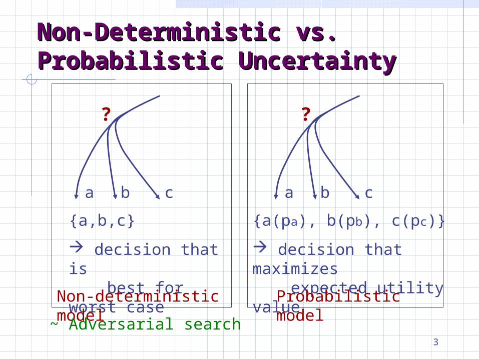
Non-Deterministic vs. Non-Deterministic vs. Probabilistic UncertaintyProbabilistic Uncertainty
?
ba c
{a,b,c}
decision that is best for worst case
?
ba c
{a(pa), b(pb), c(pc)}
decision that maximizes expected utility valueNon-deterministic
modelProbabilistic model~ Adversarial search
3
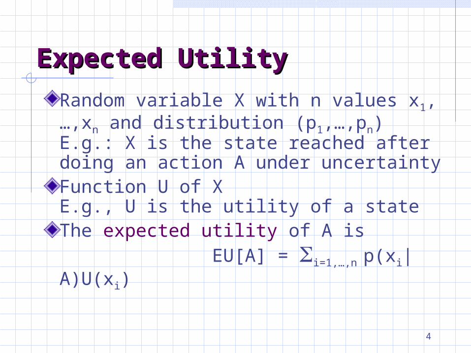
Expected UtilityExpected Utility
Random variable X with n values x1,…,xn and distribution (p1,…,pn)E.g.: X is the state reached after doing an action A under uncertaintyFunction U of XE.g., U is the utility of a stateThe expected utility of A is EU[A] = i=1,…,n p(xi|A)U(xi)
4

s0
s3s2s1
A1
0.2 0.7 0.1100 50 70
U(A1, S0) = 100 x 0.2 + 50 x 0.7 + 70 x 0.1 = 20 + 35 + 7 = 62
One State/One Action One State/One Action ExampleExample
5
s0
s3s2s1
A1
0.2 0.7 0.1100 50 70
A2
s40.2 0.8
80
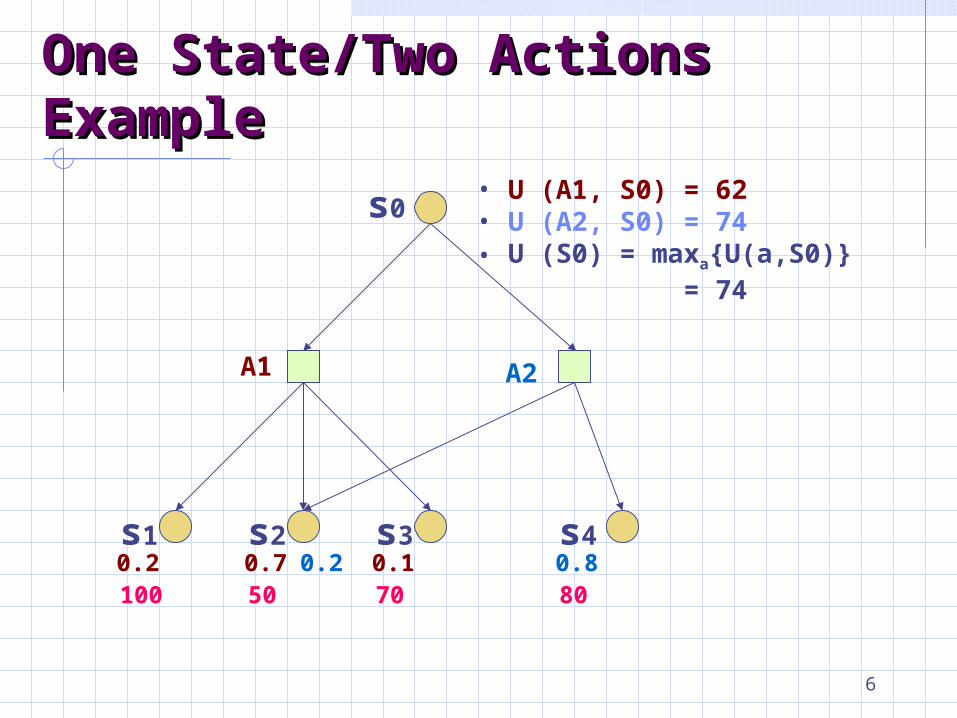
• U (A1, S0) = 62• U (A2, S0) = 74• U (S0) = maxa{U(a,S0)} = 74
One State/Two Actions One State/Two Actions ExampleExample
6

s0
s3s2s1
A1
0.2 0.7 0.1100 50 70
A2
s40.2 0.8
80
• U (A1, S0) = 62 – 5 = 57• U (A2, S0) = 74 – 25 = 49• U (S0) = maxa{U(a, S0)} = 57
-5 -25
Introducing Action CostsIntroducing Action Costs
7

MEU Principle
A rational agent should choose the action that maximizes agent’s expected utilityThis is the basis of the field of decision theoryThe MEU principle provides a normative criterion for rational choice of action
8

Not quite…
Must have a complete model of: Actions Utilities States
Even if you have a complete model, decision making is computationally intractableIn fact, a truly rational agent takes into account the utility of reasoning as well (bounded rationality)Nevertheless, great progress has been made in this area recently, and we are able to solve much more complex decision-theoretic problems than ever before
9

Axioms of Utility Theory
Orderability (A>B) (A<B) (A~B)
Transitivity (A>B) (B>C) (A>C)
Continuity A>B>C p [p,A; 1-p,C] ~ B
Substitutability A~B [p,A; 1-p,C]~[p,B; 1-p,C]
Monotonicity A>B (p≥q [p,A; 1-p,B] >~ [q,A; 1-q,B])
Decomposability[p,A; 1-p, [q,B; 1-q, C]] ~ [p,A; (1-p)q, B; (1-p)(1-q), C]
10

Money Versus Utility
Money <> Utility More money is better, but not always in
a linear relationship to the amount of money
Expected Monetary ValueRisk-averse: U(L) < U(SEMV(L))
Risk-seeking: U(L) > U(SEMV(L))
Risk-neutral: U(L) = U(SEMV(L))
11

Value Function
Provides a ranking of alternatives, but not a meaningful metric scaleAlso known as an “ordinal utility function”
Sometimes, only relative judgments (value functions) are necessaryAt other times, absolute judgments (utility functions) are required
12
Multiattribute Utility Theory
A given state may have multiple utilities ...because of multiple evaluation criteria ...because of multiple agents (interested
parties) with different utility functions
We will talk about this more later in the semester, when we discuss multi-agent systems and game theory
13
Decision Networks
Extend BNs to handle actions and utilitiesAlso called influence diagramsUse BN inference methods to solvePerform Value of Information calculations
14

Decision Networks cont.
Chance nodes: random variables, as in BNsDecision nodes: actions that a decision maker can takeUtility/value nodes: the utility of an outcome state
15
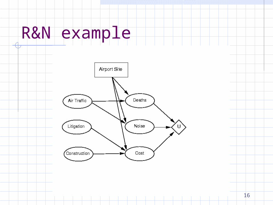
R&N example
16
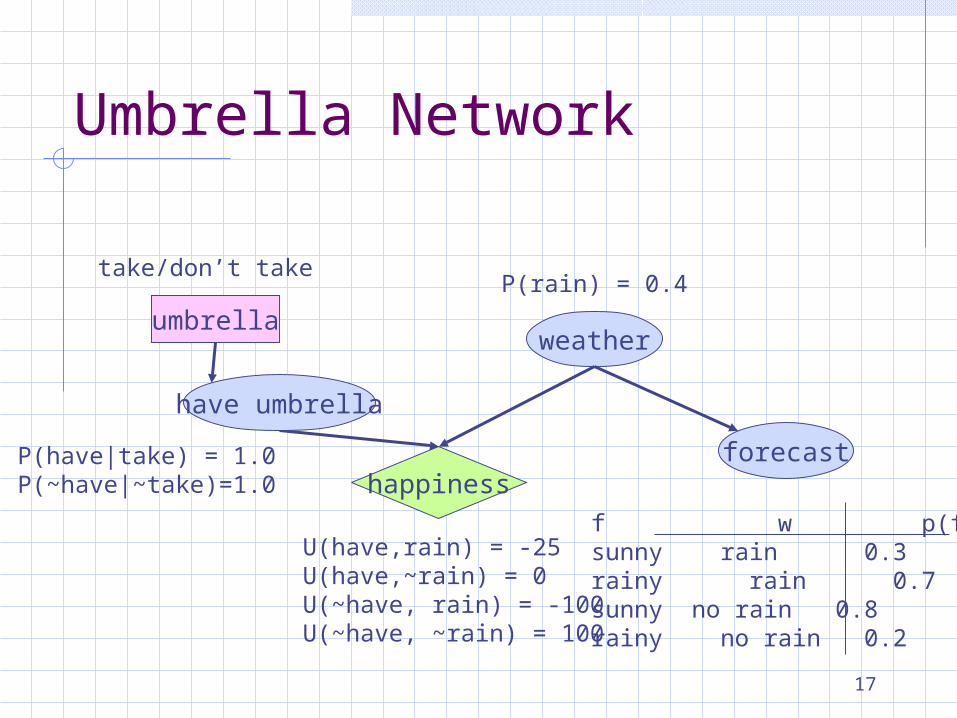
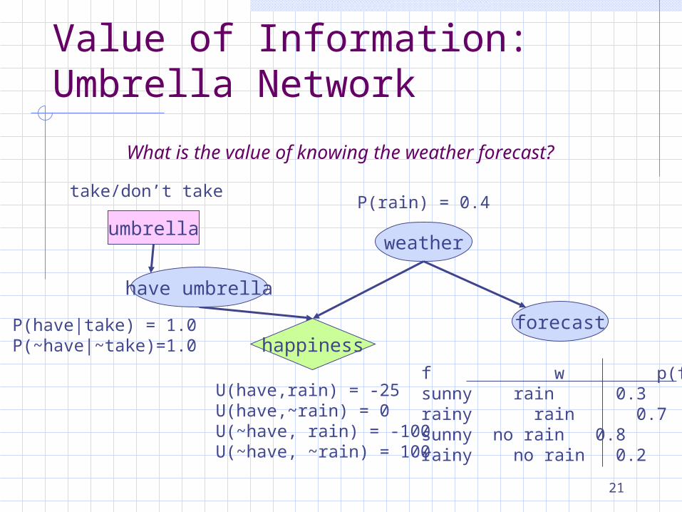
Umbrella Network
weather
forecast
umbrella
happiness
take/don’t take
f w p(f|w)sunny rain 0.3rainy rain 0.7sunny no rain 0.8rainy no rain 0.2
P(rain) = 0.4
U(have,rain) = -25U(have,~rain) = 0U(~have, rain) = -100U(~have, ~rain) = 100
have umbrella
P(have|take) = 1.0P(~have|~take)=1.0
17

Evaluating Decision Networks
Set the evidence variables for current stateFor each possible value of the decision node: Set decision node to that value Calculate the posterior probability of the
parent nodes of the utility node, using BN inference
Calculate the resulting utility for each action
Return the action with the highest utility
18

Decision Making:Umbrella Network
weather
forecast
umbrella
happiness
take/don’t take
f w p(f|w)sunny rain 0.3rainy rain 0.7sunny no rain 0.8rainy no rain 0.2
P(rain) = 0.4
U(have,rain) = -25U(have,~rain) = 0U(~have, rain) = -100U(~have, ~rain) = 100
have umbrella
P(have|take) = 1.0P(~have|~take)=1.0
Should I take my umbrella??
19

Value of Information (VOI)
Suppose an agent’s current knowledge is E. The value of the current best action is:
€
EU(α | E) = maxA
U(Resulti(A)) P(Resulti(A) | E,Do(A))i
∑
The value of the new best action (after new evidence E’ is obtained):
€
EU( ′ α | E, ′ E ) = maxA
U(Resulti(A)) P(Resulti(A) | E, ′ E ,Do(A))i
∑
The value of information for E’ is therefore:
€
VOI( ′ E ) = P(ek | E) EU(α ek | ek, E)k
∑ − EU(α | E)
20
Value of Information:Umbrella Network
weather
forecast
umbrella
happiness
take/don’t take
f w p(f|w)sunny rain 0.3rainy rain 0.7sunny no rain 0.8rainy no rain 0.2
P(rain) = 0.4
U(have,rain) = -25U(have,~rain) = 0U(~have, rain) = -100U(~have, ~rain) = 100
have umbrella
P(have|take) = 1.0P(~have|~take)=1.0
What is the value of knowing the weather forecast?
21

Sequential Decision Making
Finite HorizonInfinite Horizon
22
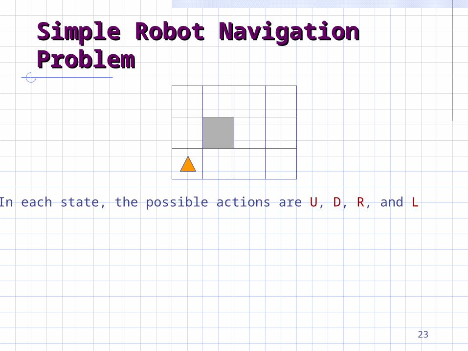
Simple Robot Navigation Simple Robot Navigation ProblemProblem
• In each state, the possible actions are U, D, R, and L
23

Probabilistic Transition Probabilistic Transition ModelModel
• In each state, the possible actions are U, D, R, and L• The effect of U is as follows (transition model):
• With probability 0.8, the robot moves up one square (if the robot is already in the top row, then it does not move)
24

Probabilistic Transition Probabilistic Transition ModelModel
• In each state, the possible actions are U, D, R, and L• The effect of U is as follows (transition model):
• With probability 0.8 the robot moves up one square (if the robot is already in the top row, then it does not move)• With probability 0.1 the robot moves right one square (if the robot is already in the rightmost row, then it does not move)
25

Probabilistic Transition Probabilistic Transition ModelModel
• In each state, the possible actions are U, D, R, and L• The effect of U is as follows (transition model):
• With probability 0.8 the robot moves up one square (if the robot is already in the top row, then it does not move)• With probability 0.1 the robot moves right one square (if the robot is already in the rightmost row, then it does not move)• With probability 0.1 the robot moves left one square (if the robot is already in the leftmost row, then it does not move)
26

Markov PropertyMarkov Property
The transition properties depend only on the current state, not on the previous history (how that state was reached)
27

Sequence of ActionsSequence of Actions
• Planned sequence of actions: (U, R)
2
3
1
4321
[3,2]
28
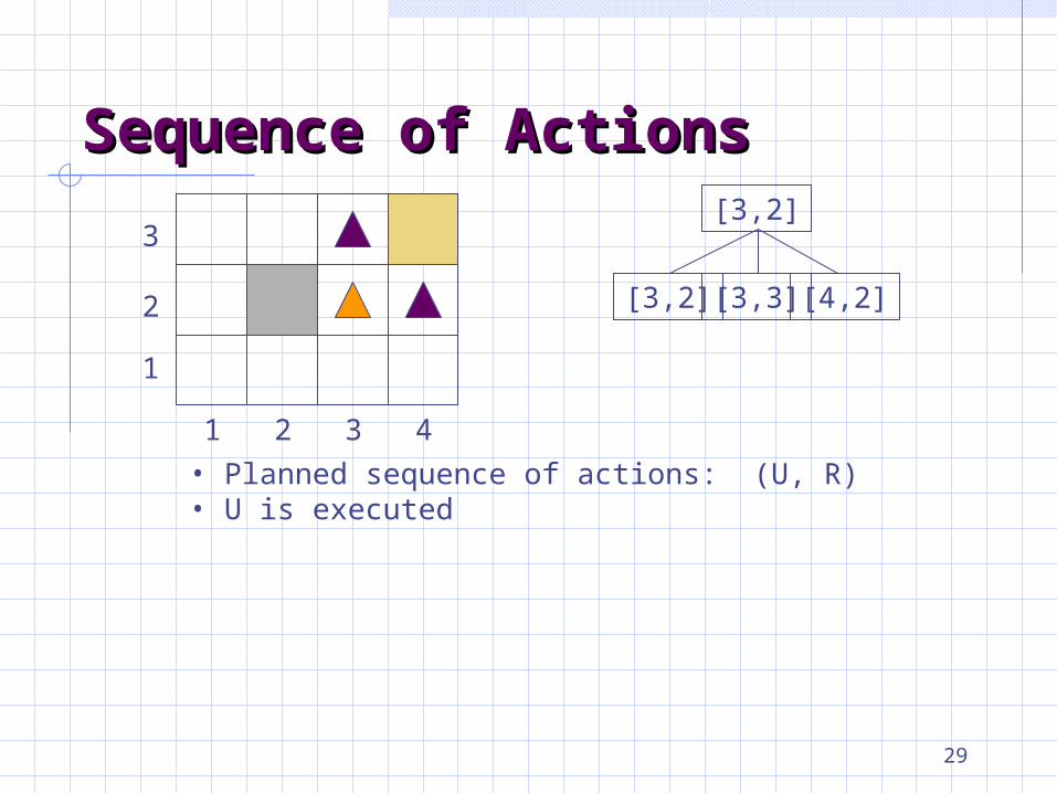
Sequence of ActionsSequence of Actions
• Planned sequence of actions: (U, R)• U is executed
2
3
1
4321
[3,2]
[4,2][3,3][3,2]
29

HistoriesHistories
• Planned sequence of actions: (U, R)• U has been executed• R is executed
• There are 9 possible sequences of states – called histories – and 6 possible final states for the robot!
4321
2
3
1
[3,2]
[4,2][3,3][3,2]
[3,3][3,2] [4,1] [4,2] [4,3][3,1]
30

Probability of Reaching the Probability of Reaching the GoalGoal
•P([4,3] | (U,R).[3,2]) = P([4,3] | R.[3,3]) x P([3,3] | U.[3,2]) + P([4,3] | R.[4,2]) x P([4,2] | U.[3,2])
2
3
1
4321
Note importance of Markov property in this derivation
•P([3,3] | U.[3,2]) = 0.8•P([4,2] | U.[3,2]) = 0.1
•P([4,3] | R.[3,3]) = 0.8•P([4,3] | R.[4,2]) = 0.1
•P([4,3] | (U,R).[3,2]) = 0.6531

Utility FunctionUtility Function
• [4,3] provides power supply• [4,2] is a sand area from which the robot cannot escape
-1
+1
2
3
1
4321
32
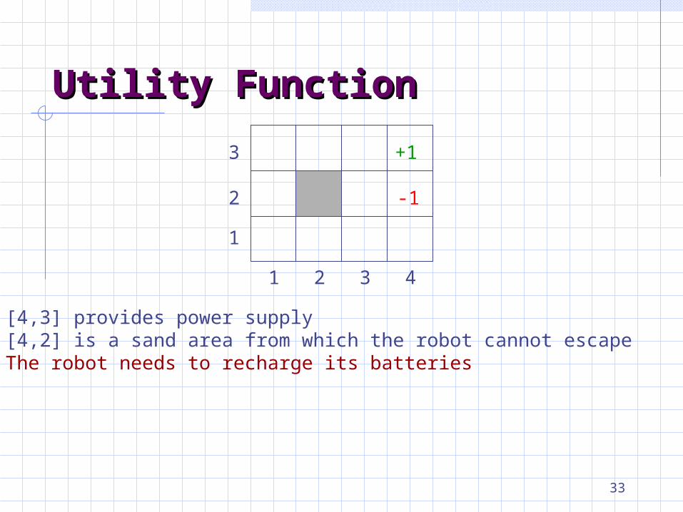
Utility FunctionUtility Function
• [4,3] provides power supply• [4,2] is a sand area from which the robot cannot escape• The robot needs to recharge its batteries
-1
+1
2
3
1
4321
33
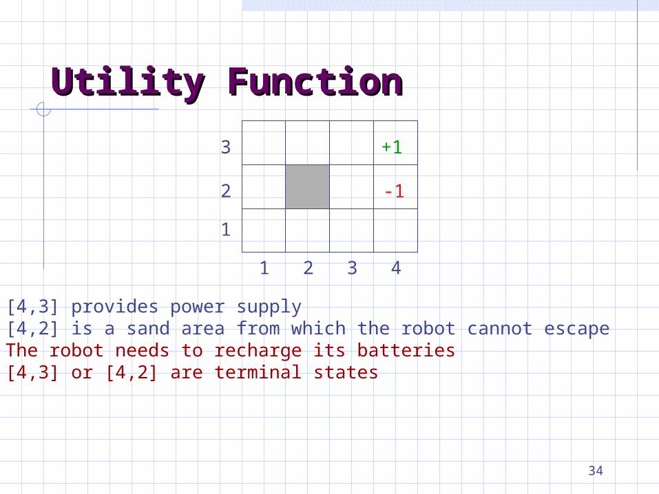
Utility FunctionUtility Function
• [4,3] provides power supply• [4,2] is a sand area from which the robot cannot escape• The robot needs to recharge its batteries• [4,3] or [4,2] are terminal states
-1
+1
2
3
1
4321
34

Utility of a HistoryUtility of a History
• [4,3] provides power supply• [4,2] is a sand area from which the robot cannot escape• The robot needs to recharge its batteries• [4,3] or [4,2] are terminal states• The utility of a history is defined by the utility of the last state (+1 or –1) minus n/25, where n is the number of moves
-1
+1
2
3
1
4321
35
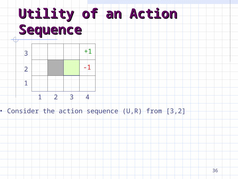
Utility of an Action Utility of an Action SequenceSequence
-1
+1
• Consider the action sequence (U,R) from [3,2]
2
3
1
4321
36
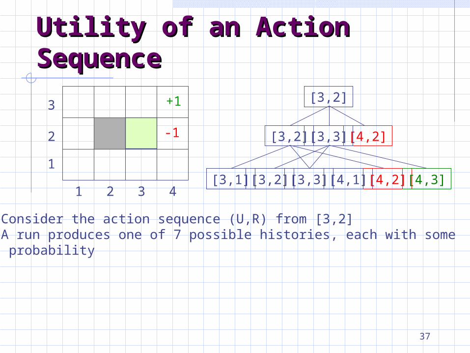
Utility of an Action Utility of an Action SequenceSequence
-1
+1
• Consider the action sequence (U,R) from [3,2]• A run produces one of 7 possible histories, each with some probability
2
3
1
4321
[3,2]
[4,2][3,3][3,2]
[3,3][3,2] [4,1] [4,2] [4,3][3,1]
37

Utility of an Action Utility of an Action SequenceSequence
-1
+1
• Consider the action sequence (U,R) from [3,2]• A run produces one among 7 possible histories, each with some probability• The utility of the sequence is the expected utility of the histories:
U = hUh P(h)
2
3
1
4321
[3,2]
[4,2][3,3][3,2]
[3,3][3,2] [4,1] [4,2] [4,3][3,1]
38

Optimal Action SequenceOptimal Action Sequence
-1
+1
• Consider the action sequence (U,R) from [3,2]• A run produces one among 7 possible histories, each with some probability• The utility of the sequence is the expected utility of the histories• The optimal sequence is the one with maximal utility
2
3
1
4321
[3,2]
[4,2][3,3][3,2]
[3,3][3,2] [4,1] [4,2] [4,3][3,1]
39
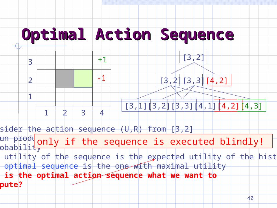
Optimal Action SequenceOptimal Action Sequence
-1
+1
• Consider the action sequence (U,R) from [3,2]• A run produces one among 7 possible histories, each with some probability• The utility of the sequence is the expected utility of the histories• The optimal sequence is the one with maximal utility• But is the optimal action sequence what we want to compute?
2
3
1
4321
[3,2]
[4,2][3,3][3,2]
[3,3][3,2] [4,1] [4,2] [4,3][3,1]
only if the sequence is executed blindly!
40
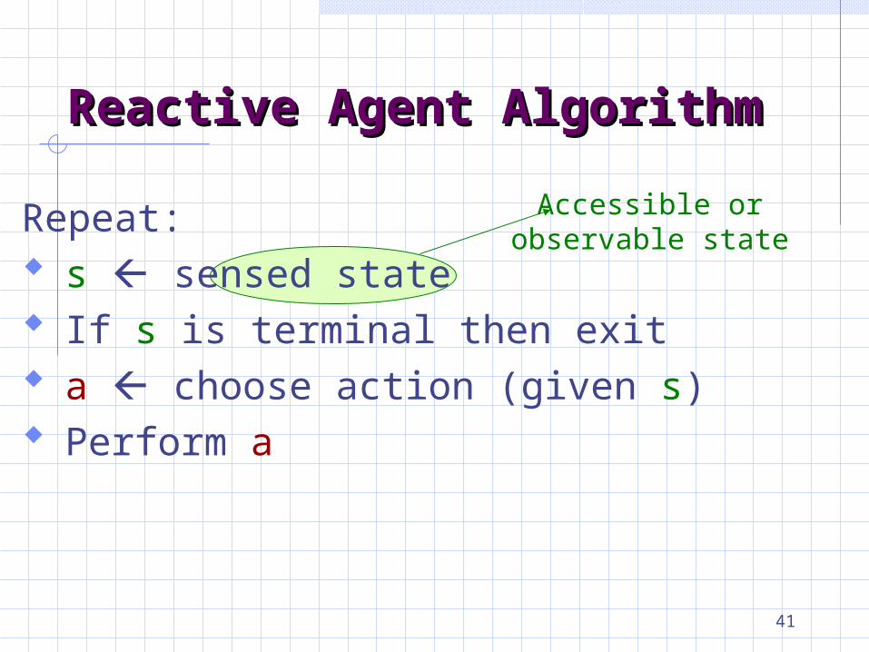
Accessible orobservable state
Repeat: s sensed state If s is terminal then exit a choose action (given s) Perform a
Reactive Agent AlgorithmReactive Agent Algorithm
41

Policy Policy (Reactive/Closed-Loop (Reactive/Closed-Loop Strategy)Strategy)
• A policy is a complete mapping from states to actions
-1
+1
2
3
1
4321
42

Repeat: s sensed state If s is terminal then exit a (s) Perform a
Reactive Agent AlgorithmReactive Agent Algorithm
43

Optimal PolicyOptimal Policy
-1
+1
• A policy is a complete mapping from states to actions• The optimal policy * is the one that always yields a history (ending at a terminal state) with maximal expected utility
2
3
1
4321
Makes sense because of Markov property
Note that [3,2] is a “dangerous” state that the optimal policy
tries to avoid
44

Optimal PolicyOptimal Policy
-1
+1
• A policy is a complete mapping from states to actions• The optimal policy * is the one that always yields a history with maximal expected utility
2
3
1
4321
This problem is called aMarkov Decision Problem (MDP)
How to compute *?45

Additive UtilityAdditive Utility
History H = (s0,s1,…,sn)
The utility of H is additive iff: U(s0,s1,…,sn) = R(0) + U(s1,…,sn) = R(i)
Reward
46

Additive UtilityAdditive Utility
History H = (s0,s1,…,sn)
The utility of H is additive iff: U(s0,s1,…,sn) = R(0) + U(s1,…,sn) =
R(i)
Robot navigation example:R(n) = +1 if sn = [4,3]
R(n) = -1 if sn = [4,2]
R(i) = -1/25 if i = 0, …, n-1 47
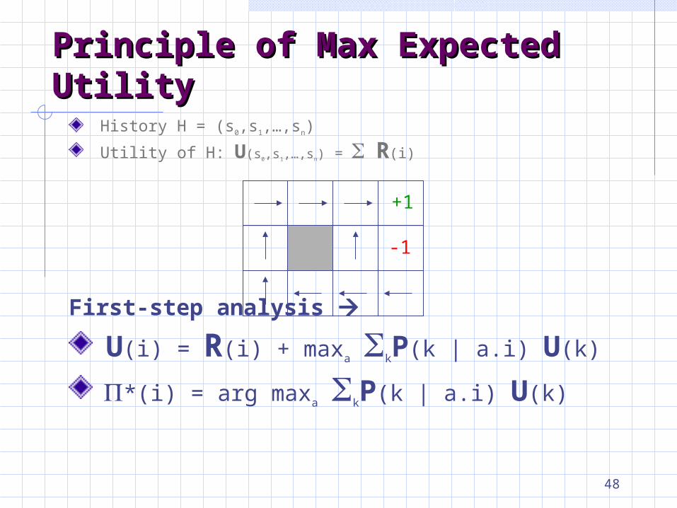
Principle of Max Expected Principle of Max Expected UtilityUtility
History H = (s0,s1,…,sn)
Utility of H: U(s0,s1,…,sn) = R(i)
First-step analysis
U(i) = R(i) + maxa kP(k | a.i) U(k)
*(i) = arg maxa kP(k | a.i) U(k)
-1
+1
48
Defining State Utility
Problem: When making a decision, we only know the
reward so far, and the possible actions We’ve defined utility retroactively (i.e., the
utility of a history is obvious once we finish it)
What is the utility of a particular state in the middle of decision making?
Need to compute expected utility of possible future histories
49

Value IterationValue Iteration Initialize the utility of each non-terminal state si
to U0(i) = 0
For t = 0, 1, 2, …, do:
Ut+1(i) R(i) + maxa kP(k | a.i) Ut(k)
-1
+1
2
3
1
4321
50

Value IterationValue Iteration Initialize the utility of each non-terminal state si
to U0(i) = 0
For t = 0, 1, 2, …, do:
Ut+1(i) R(i) + maxa kP(k | a.i) Ut(k)
Ut([3,1])
t0 302010
0.6110.5
0-1
+1
2
3
1
4321
0.705 0.655 0.3880.611
0.762
0.812 0.868 0.918
0.660
Note the importanceof terminal states andconnectivity of thestate-transition graph
51

Policy IterationPolicy Iteration
Pick a policy at random
52

Policy IterationPolicy Iteration
Pick a policy at random Repeat: Compute the utility of each state for Ut+1(i) R(i) + kP(k | (i).i) Ut(k)
53

Policy IterationPolicy Iteration
Pick a policy at random Repeat:
Compute the utility of each state for Ut+1(i) R(i) + kP(k | (i).i) Ut(k)
Compute the policy ’ given these utilities
’(i) = arg maxa kP(k | a.i) U(k)
54

Policy IterationPolicy Iteration
Pick a policy at random Repeat: Compute the utility of each state for
Ut+1(i) R(i) + kP(k | (i).i) Ut(k) Compute the policy ’ given these
utilities
’(i) = arg maxa kP(k | a.i) U(k)
If ’ = then return
Or solve the set of linear equations:
U(i) = R(i) + kP(k | (i).i) U(k)(often a sparse system)
55

Infinite HorizonInfinite Horizon
-1
+1
2
3
1
4321
In many problems, e.g., the robot navigation example, histories are potentially unbounded and the same state can be reached many timesOne trick:
Use discounting to make an infinitehorizon problem mathematicallytractable
What if the robot lives forever?
56
Top Related