


Languages
Pages
Legal

U N I T 1
DATABASE MANAGEMENT SYSTEM

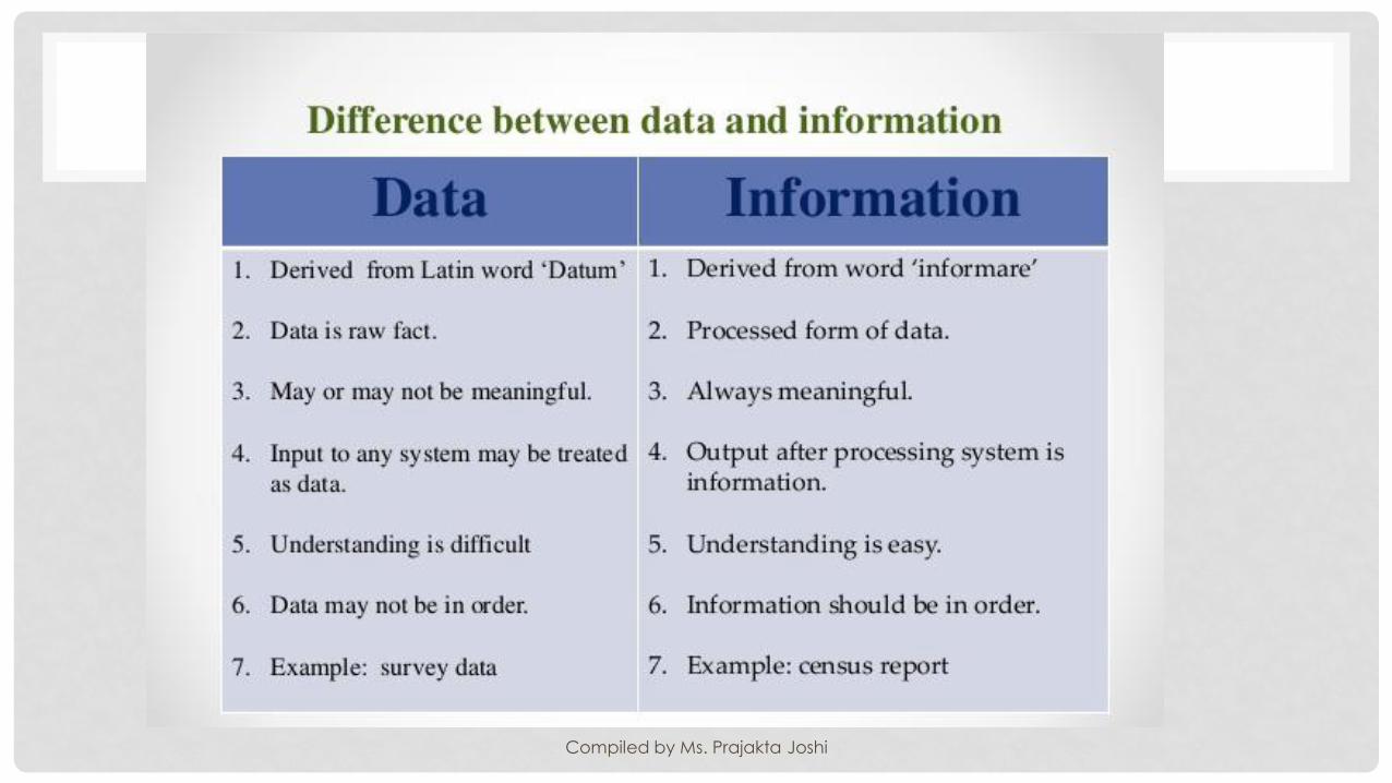
DATA
Compiled by Ms. Prajakta Joshi

INFORMATION
• Information is organised or classified data, which has some meaningful
values for the receiver.
• Information is data that has been converted into more useful or
intelligible form.
Characteristics of Information:
Timely
Accuracy
completeness
Compiled by Ms. Prajakta Joshi
Compiled by Ms. Prajakta Joshi

DATABASE
• A database is a collection of related data which represents some
aspect of the real world. A database system is designed to be built
and populated with data for a certain task
Compiled by Ms. Prajakta Joshi

Compiled by Ms. Prajakta Joshi

WHAT IS DBMS?
• Collection of interrelated data
• Set of programs to access the data
• DBMS contains information about a particular enterprise
• DBMS provides an environment that is both convenient and efficient
to use.
Compiled by Ms. Prajakta Joshi

DBMS
• DBMS is a collection of organized, interrelated data and set of programs to store the data efficiently and access those data in an easy and effective manner
A software package/ system to facilitate the creation and maintenance of a computerized database.
It
• defines (data types, structures, constraints)
• construct (storing data on some storage medium
controlled by DBMS)
• manipulate (querying, update, report generation) databases for various applications.
Compiled by Ms. Prajakta Joshi

ADVANTAGES OF DBMS
• Reduction of Redundancies
• Elimination of Inconsistencies
• Shared Data
• Integrity
• Security
• Data Independence
Physical Data Independence
Logical Data Independence
Compiled by Ms. Prajakta Joshi
DISADVANTAGES OF DBMS
• Backup and Recovery Issues
• Complexity
• Performance
• Security
• Problem associated with centralization
Compiled by Ms. Prajakta Joshi

NEED OF DBMS
• Creation of a database.
• Retrieval of information from the database.
• Updating the database.
• Managing a database.
• Storing Database
Compiled by Ms. Prajakta Joshi

APPLICATIONS OF DBMS
• Home
• Banking
• Reservation System
• Finance
• E-Commerce
• Industry
• Education
• Sales
Compiled by Ms. Prajakta Joshi

ARCHITECTURE OF DBMS
• 1. Single tier architecture
• In this type of architecture, the database is readily available on the
client machine, any request made by client doesn’t require a network
connection to perform the action on the database.
• For example, lets say you want to fetch the records of employee from
the database and the database is available on your computer
system, so the request to fetch employee details will be done by your
computer and the records will be fetched from the database by your
computer as well. This type of system is generally referred as local
database system.
Compiled by Ms. Prajakta Joshi

TWO TIER ARCHITECTURE
Compiled by Ms. Prajakta Joshi

THREE TIER ARCHITECTURE
Compiled by Ms. Prajakta Joshi

THREE LEVEL ARCHITECTURE OF DATABASE
Compiled by Ms. Prajakta Joshi

VIEW OF DATA
• Data abstraction
• Instance and schema
Compiled by Ms. Prajakta Joshi

DATA ABSTRACTION IN DBMS
• Physical level: This is the lowest
level of data abstraction. It
describes how data is actually
stored in database. You can
get the complex data structure
details at this level.
• Logical level: This is the middle
level of 3-level data abstraction
architecture. It describes what
data is stored in database.
• View level: Highest level of
data abstraction. This level
describes the user interaction
Compiled by Ms. Prajakta Joshi

INSTANCE AND SCHEMA IN DBMS
• DBMS Schema
• Definition of schema: Design
of a database is called the
schema. Schema is of three
types: Physical schema,
logical schema and view
schema.
• Physical SchemaThe design of
a database at physical level is
called physical schema, how
the data stored in blocks of
storage is described at this
Compiled by Ms. Prajakta Joshi

SCHEMAS IN DBMS
• Logical Schema:
• Design of database at
logical level is called logical
schema, programmers and
database administrators
work at this level, at this
level data can be
described as certain types
of data records gets stored
in data structures, however
the internal details such as
implementation of data
• View Schema:
• Design of database at view
level is called view schema.
This generally describes end
user interaction with
database systems.
Compiled by Ms. Prajakta Joshi

DBMS INSTANCE
• Definition of instance: The data stored in database at a particular
moment of time is called instance of database.
• Database schema defines the variable declarations in tables that
belong to a particular database; the value of these variables at a
moment of time is called the instance of that database.
Compiled by Ms. Prajakta Joshi

DATABASE LANGUAGES
Compiled by Ms. Prajakta Joshi
DATA DEFINITION LANGUAGE
• DDL stands for Data Definition Language. It is used to define database
structure or pattern.
• It is used to create schema, tables, indexes, constraints, etc. in the
database.
• Using the DDL statements, you can create the skeleton of the database.
• Data definition language is used to store the information of metadata
like the number of tables and schemas, their names, indexes, columns in
each table, constraints, etc.
• Here are some tasks that come under DDL:
• Create: It is used to create objects in the database.
• Alter: It is used to alter the structure of the database.
• Drop: It is used to delete objects from the database.
• Truncate: It is used to remove all records from a table.
• Rename: It is used to rename an object.Compiled by Ms. Prajakta Joshi

DATA MANIPULATION LANGUAGE
• DML stands for Data Manipulation Language. It is used for accessing
and manipulating data in a database. It handles user requests.
• Here are some tasks that come under DML:
• Select: It is used to retrieve data from a database.
• Insert: It is used to insert data into a table.
• Update: It is used to update existing data within a table.
• Delete: It is used to delete all records from a table.
• Merge: It performs UPSERT operation, i.e., insert or update operations.
• Call: It is used to call a structured query language or a Java
subprogram.
• Explain Plan: It has the parameter of explaining data.
• Lock Table: It controls concurrency.
Compiled by Ms. Prajakta Joshi

DATA CONTROL LANGUAGE
• DCL stands for Data Control Language. It is used to retrieve the stored or saved
data.
• The DCL execution is transactional. It also has rollback parameters.
• (But in Oracle database, the execution of data control language does not have
the feature of rolling back.)
• Here are some tasks that come under DCL:
• Grant: It is used to give user access privileges to a database.
• Revoke: It is used to take back permissions from the user.
• There are the following operations which have the authorization of Revoke:
• CONNECT, INSERT, USAGE, EXECUTE, DELETE, UPDATE and SELECT.
Compiled by Ms. Prajakta Joshi
TRANSACTION CONTROL LANGUAGE
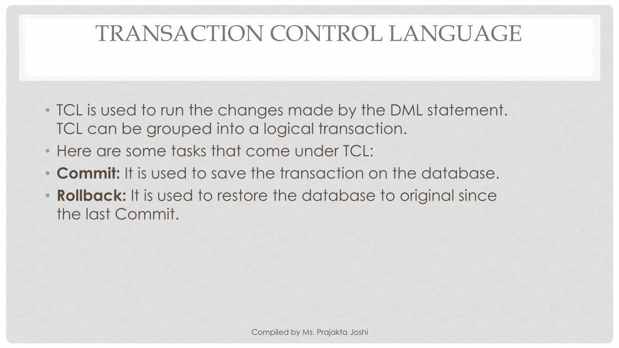
• TCL is used to run the changes made by the DML statement.
TCL can be grouped into a logical transaction.
• Here are some tasks that come under TCL:
• Commit: It is used to save the transaction on the database.
• Rollback: It is used to restore the database to original since
the last Commit.
Compiled by Ms. Prajakta Joshi

FILE PROCESSING SYSTEM
• A file processing system helps people keep track of files as
they move throughout the various departments of a business.
• It should be recorded in such a way that
• Should be able to get the data any point in time latter
• Should be able to add details to it whenever required
• Should be able to modify stored information, as needed
• Should also be able to delete them
Compiled by Ms. Prajakta Joshi

DISADVANTAGES OF FILE PROCESSING SYSTEM
• Data Redundancy
• Data Inconsistency
• Difficult in Accessing Data
• Integrity Problem
• Data Isolation
• Concurrent Access Problem
• Atomicity Problem
Compiled by Ms. Prajakta Joshi

Compiled by Ms. Prajakta Joshi

TRANSACTION MANAGEMENT
• A transaction is a logical unit of work that contains one or more SQL
statements
• It is a collection of operations that performs a single logical function
in a database application
• A transaction is an atomic unit
• Transactions in a database environment have two main purposes:
• Reliability of data
• Concurrent Access of Data
Compiled by Ms. Prajakta Joshi

DATA MODELS
• Data models can facilitate interaction among the designer, the
application programmer and the end user.
• A well- developed data model can even foster improved
understanding of the organization for which the database design is
developed.
• Data models are a communication tool.
Compiled by Ms. Prajakta Joshi

IMPORTANCE OF DATA MODELS
• The data model is the blueprint.
• The data model is the requirements.
• The data model is the specifications.
• The data model is reusable.
Compiled by Ms. Prajakta Joshi

THE BASIC BUILDING BLOCKS OF DATA MODELS
• The basic building blocks of all data models are entities,
attributes, and relationships.
• An entity is anything, such as a person, place, thing, or event,
about which data are to be collected and stored. Entities may
be physical objects such as customers or products. But entities
may also be abstractions such as flight routes or musical
concerts.
• An attribute is a characteristic of an entity. For example, a
CUSTOMER entity would be described by attributes such as
customer last name, customer first name, customer phone,
customer address, and customer credit limit. The attributes are
the equivalent of fields in file systems.
Compiled by Ms. Prajakta Joshi

TYPES OF RELATIONS
• One-to-many (1:M) relationship. A painter paints many different paintings, but each one of them is painted by only one painter. Thus the painter (the “one”) is related to the paintings (the “many”). Therefore, database designers label the relationship “PAINTER paints PAINTING” as 1:M. Similarly, a customer (the “one”) might generate many invoices, but each invoice (the “many”) is generated by only a single customer. The “CUSTOMER generates INVOICE” relationship would also be labeled 1:M.
• Many-to-many (M:N or M:M) relationship. An employee might learn many job skills, and each job skill might be learned by many employees. Database designers label the relationship “EMPLOYEE learns SKILL” as M:N. Similarly, a student can take many classes, and each class can be taken by many students, thus yielding the M:N relationship label for the relationship expressed by “STUDENT
Compiled by Ms. Prajakta Joshi

Compiled by Ms. Prajakta Joshi
U N I T 2
DATABASE MANAGEMENT SYSTEM

KEYS
• Candidate Key - The candidate keys in a table are defined as the set of keys that is minimal and can uniquely identify any data row in the table.
• Primary Key - The primary key is selected from one of the candidate keys and becomes the identifying key of a table. It can uniquely identify any data row of the table.
• Super Key - Super Key is the superset of primary key. The super key contains a set of attributes, including the primary key, which can uniquely identify any data row in the table.
• Composite Key - If any single attribute of a table is not capable of being the key i.e it cannot identify a row uniquely, then we combine two or more attributes to form a key. This is known as a composite key.
• Secondary Key - Only one of the candidate keys is selected as the primary key. The rest of them are known as secondary keys.
• Foreign Key - A foreign key is an attribute value in a table that acts as the primary key in another another. Hence, the foreign key is useful in linking together two tables. Data should be entered in the foreign key column with great care, as wrongly entered data can invalidate the relationship between the two tables.
Compiled by Ms. Prajakta Joshi

NORMALIZATION
• If a database design is not perfect, it may contain anomalies, which are like a bad dream for any database administrator. Managing a database with anomalies is next to impossible.
• Update anomalies − If data items are scattered and are not linked to each other properly, then it could lead to strange situations. For example, when we try to update one data item having its copies scattered over several places, a few instances get updated properly while a few others are left with old values. Such instances leave the database in an inconsistent state.
• Deletion anomalies − We tried to delete a record, but parts of it was left undeleted because of unawareness, the data is also saved somewhere else.
• Insert anomalies − We tried to insert data in a record that does not exist at all.
Compiled by Ms. Prajakta Joshi
FIRST NORMAL FORM
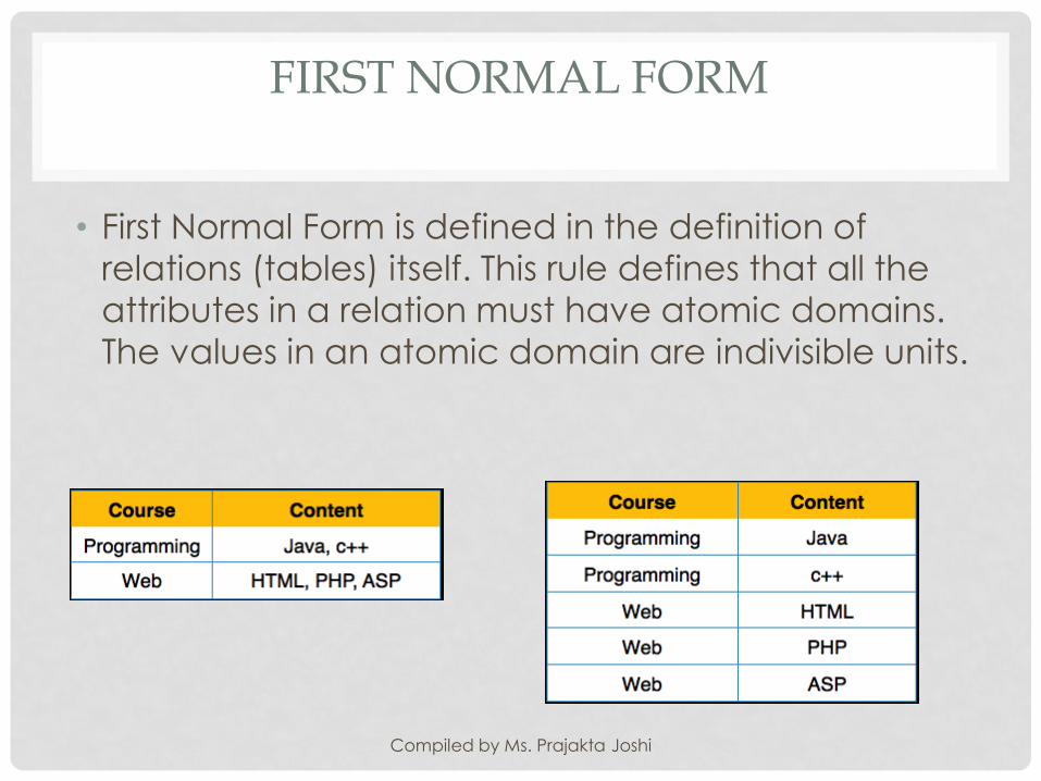
• First Normal Form is defined in the definition of
relations (tables) itself. This rule defines that all the
attributes in a relation must have atomic domains.
The values in an atomic domain are indivisible units.
Compiled by Ms. Prajakta Joshi

SECOND NORMAL FORM
• Before we learn about the second normal form, we need to understand the following −
• Prime attribute − An attribute, which is a part of the candidate-key, is known as a prime attribute.
• Non-prime attribute − An attribute, which is not a part of the prime-key, is said to be a non-prime attribute.
• If we follow second normal form, then every non-prime attribute should be fully functionally dependent on prime key attribute. That is, if X → A holds, then there should not be any proper subset Y of X, for which Y → A also holds true.
Compiled by Ms. Prajakta Joshi
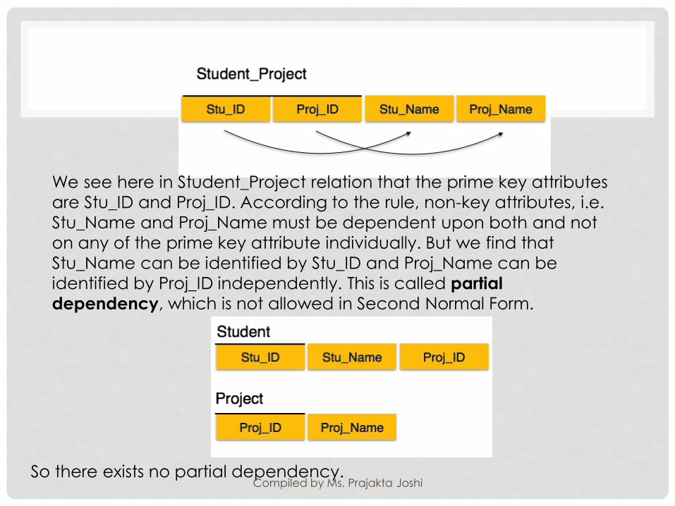
We see here in Student_Project relation that the prime key attributes
are Stu_ID and Proj_ID. According to the rule, non-key attributes, i.e.
Stu_Name and Proj_Name must be dependent upon both and not
on any of the prime key attribute individually. But we find that
Stu_Name can be identified by Stu_ID and Proj_Name can be
identified by Proj_ID independently. This is called partial
dependency, which is not allowed in Second Normal Form.
So there exists no partial dependency.Compiled by Ms. Prajakta Joshi

THIRD NORMAL FORM
• For a relation to be in Third Normal Form, it must be
in Second Normal form and the following must
satisfy −
• No non-prime attribute is transitively dependent on
prime key attribute.
• For any non-trivial functional dependency, X → A,
then either −
• X is a superkey or,
• A is prime attribute.
Compiled by Ms. Prajakta Joshi

We find that in the above Student_detail relation, Stu_ID is the
key and only prime key attribute. We find that City can be
identified by Stu_ID as well as Zip itself. Neither Zip is a superkey
nor is City a prime attribute. Additionally, Stu_ID → Zip → City, so
there exists transitive dependency.
To bring this relation into third normal form, we break the
relation into two relations as follows −
Compiled by Ms. Prajakta Joshi
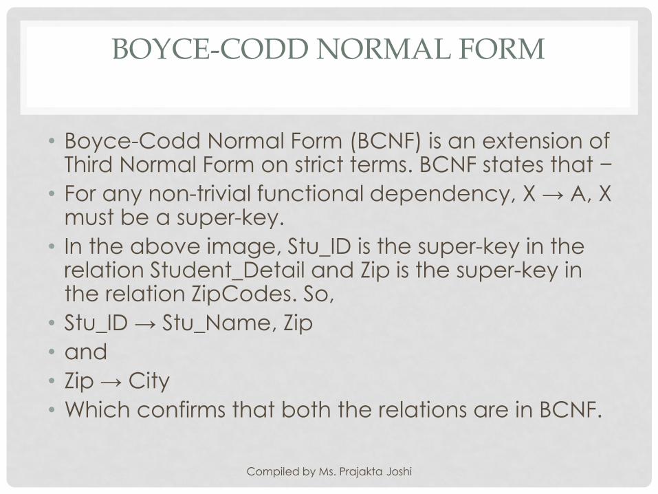
BOYCE-CODD NORMAL FORM
• Boyce-Codd Normal Form (BCNF) is an extension of Third Normal Form on strict terms. BCNF states that −
• For any non-trivial functional dependency, X → A, X must be a super-key.
• In the above image, Stu_ID is the super-key in the relation Student_Detail and Zip is the super-key in the relation ZipCodes. So,
• Stu_ID → Stu_Name, Zip
• and
• Zip → City
• Which confirms that both the relations are in BCNF.
Compiled by Ms. Prajakta Joshi
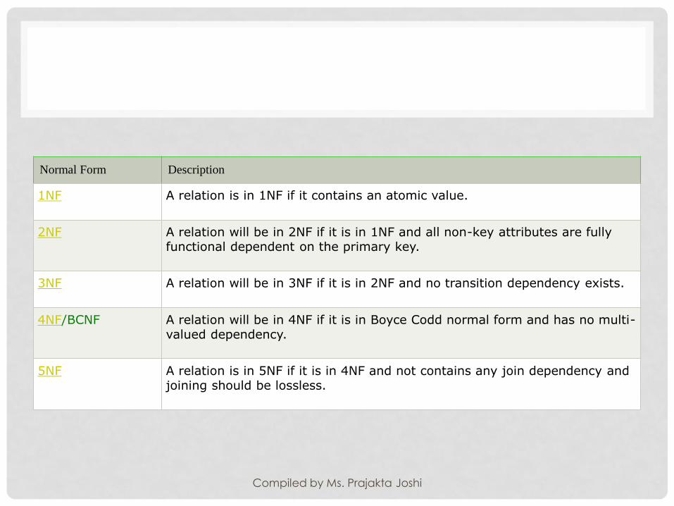
Normal Form Description
1NF A relation is in 1NF if it contains an atomic value.
2NF A relation will be in 2NF if it is in 1NF and all non-key attributes are fully functional dependent on the primary key.
3NF A relation will be in 3NF if it is in 2NF and no transition dependency exists.
4NF/BCNF A relation will be in 4NF if it is in Boyce Codd normal form and has no multi-valued dependency.
5NF A relation is in 5NF if it is in 4NF and not contains any join dependency and joining should be lossless.
Compiled by Ms. Prajakta Joshi
COLUMN ATTRIBUTE
UNSIGNED
• Unsigned allows us to enter positive value; you cannot give any negative number
NOT NULL
• Means column can not be empty
DEFAULT
• It is used to give a column a fixed value.
AUTO_INCREMENT
Auto-increment allows a unique number to be generated automatically when a new record is inserted into a table.
• Often this is the primary key field that we would like to be created automatically every time a new record is inserted.
Compiled by Ms. Prajakta Joshi

ALTER
alter table fyit
add fee decimal(4,2) unsigned default 2050;
describe fyit;
alter table fyit
add fee decimal(4,2) unsigned default 2050 after
Std_name;
Compiled by Ms. Prajakta Joshi

CHANGE(CHANGING COLUMN NAME)
Alter table fyit
change fee Tution_Fee decimal(4,2) unsigned default
2050;
Compiled by Ms. Prajakta Joshi

DELETING COLUMN
Alter table fyit
drop Tution_Fee decimal(4,2) unsigned default 2050;
Compiled by Ms. Prajakta Joshi

DELETE/ADD PRIMARY KEY
desc fyit;
alter table fyit
Drop primary key;
alter table fyit
add primary key(std_id);
Compiled by Ms. Prajakta Joshi

RENAMING TABLE
alter table fyit rename fybscit;
Or
Rename table fyit to fybscit;
Compiled by Ms. Prajakta Joshi

BUILT IN FUNCTIONS(STRING)
Compiled by Ms. Prajakta Joshi

Compiled by Ms. Prajakta Joshi

Compiled by Ms. Prajakta Joshi

BUILT IN FUNCTIONS(DATE FUNCTIONS)
Compiled by Ms. Prajakta Joshi

Compiled by Ms. Prajakta Joshi

Compiled by Ms. Prajakta Joshi

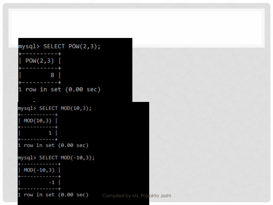
NUMERICAL FUNCTION
Compiled by Ms. Prajakta Joshi
Compiled by Ms. Prajakta Joshi

Compiled by Ms. Prajakta Joshi

Compiled by Ms. Prajakta Joshi
Compiled by Ms. Prajakta Joshi

Compiled by Ms. Prajakta Joshi

Compiled by Ms. Prajakta Joshi

RELATIONAL ALGEBRA• Relational database systems are expected to be equipped with
a query language that can assist its users to query the database instances. There are two kinds of query languages − relational algebra and relational calculus.
• Relational algebra is a procedural query language, which takes instances of relations as input and yields instances of relations as output.
• It uses operators to perform queries. An operator can be either unary or binary.
• They accept relations as their input and yield relations as their output.
• Relational algebra is performed recursively on a relation and intermediate results are also considered relations.
Compiled by Ms. Prajakta Joshi

THE FUNDAMENTAL OPERATIONS OF RELATIONAL ALGEBRA ARE AS
FOLLOWS −
• Select
• Project
• Union
• Set different
• Cartesian product
• Rename
Compiled by Ms. Prajakta Joshi

SELECT OPERATION (Σ)
• It selects tuples that satisfy the given predicate from
a relation.
• Notation − σp(r)
• Where σ stands for selection predicate and r stands
for relation. p is prepositional logic formula which
may use connectors like and, or, and not. These
terms may use relational operators like − =, ≠, ≥, <
, >, ≤.
Compiled by Ms. Prajakta Joshi

EXAMPLE
Example :
R
(A B C)
----------
1 2 4
2 2 3
3 2 3
4 3 4
• π (σ (c>3)R ) will show following tuples.
• A B C
• -------
• 1 2 4
• 4 3 4
Compiled by Ms. Prajakta Joshi

PROJECT OPERATION (∏)
• Projection is used to project required column data from a
relation.
• It projects column(s) that satisfy a givenpredicate.
• Notation − ∏A1, A2, An (r)• Where A1, A2 , An are attribute names of relation r.
• Duplicate rows are automatically eliminated, asrelation is a set.
Compiled by Ms. Prajakta Joshi

EXAMPLE
R
(A B C)
----------
1 2 4
2 2 3
3 2 3
4 3 4
π (BC)
B C
-----
2 4
2 3
3 4
Compiled by Ms. Prajakta Joshi

UNION OPERATION
• Notation − r U s
• Where r and s are either database relations or relation result set (temporary relation).
• For a union operation to be valid, the following conditions must hold −
• r, and s must have the same number of attributes.
• Attribute domains must be compatible.
• Duplicate tuples are automatically eliminated.
Compiled by Ms. Prajakta Joshi

EXAMPLE
∏ author (Books) ∪ ∏ author (Articles)Output − Projects the names of the authors who have either written a book or an article or both.
Output − Projects the names of the authors who have either written a book or an article or both.
Compiled by Ms. Prajakta Joshi

SET DIFFERENCE (−)
• The result of set difference operation is tuples, which
are present in one relation but are not in the
second relation.
• Notation − r − s
• Finds all the tuples that are present in r but not in s.
Compiled by Ms. Prajakta Joshi
EXAMPLE
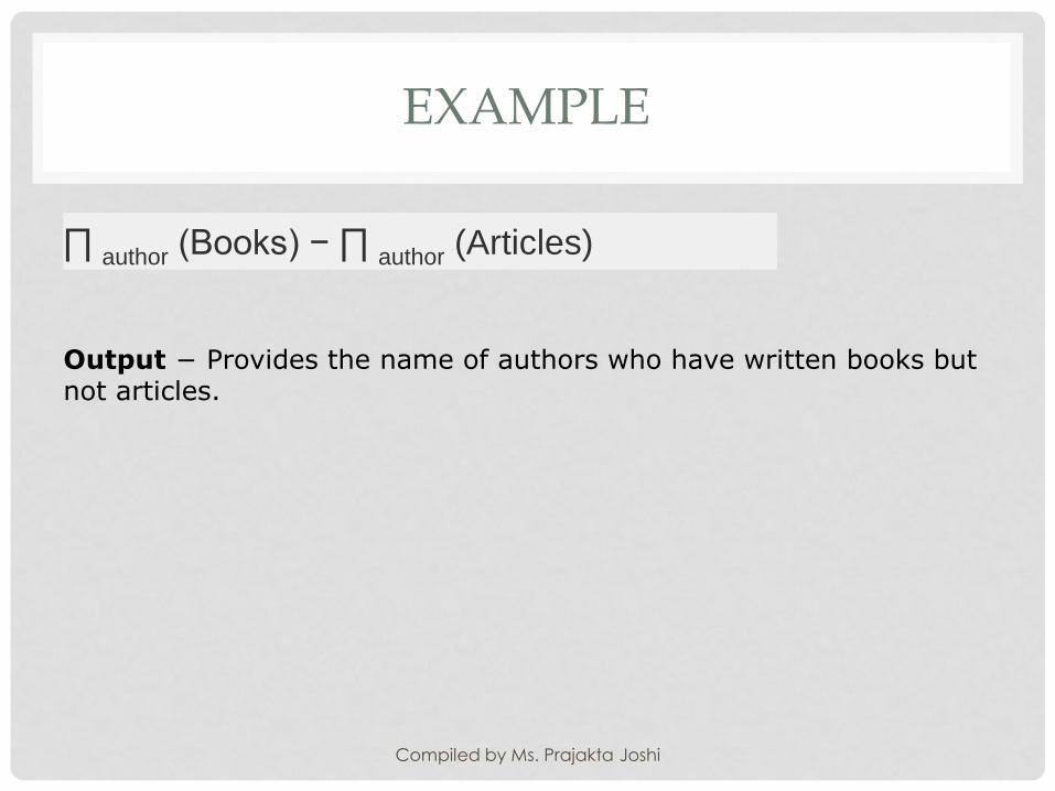
∏ author (Books) − ∏ author (Articles)
Output − Provides the name of authors who have written books but not articles.
Compiled by Ms. Prajakta Joshi

CARTESIAN PRODUCT (Χ)
• Combines information of two different relations into
one.
• Notation − r Χ s
• Where r and s are relations and their output will be
defined as −
• r Χ s = { q t | q ∈ r and t ∈ s}
Compiled by Ms. Prajakta Joshi

σauthor = ‘Raheja'(Books Χ Articles)
Output − Yields a relation, which shows all the books and articles written by Raheja.
Compiled by Ms. Prajakta Joshi

RENAME OPERATION (Ρ)
• The results of relational algebra are also relations but without any name. The rename operation allows us to rename the output relation. 'rename' operation is denoted with small Greek letter rho ρ.
• Notation − ρ x (E)
• Where the result of expression E is saved with name of x.
Compiled by Ms. Prajakta Joshi

UPDATE AND SET
Compiled by Ms. Prajakta Joshi

Compiled by Ms. Prajakta Joshi

• Update Dept
• Set salary = salary+1000
• Where city =“Mumbai”;
Compiled by Ms. Prajakta Joshi

JOIN
• A relational database consists of multiple related tables linking together using common columns which are known as foreign key columns. Because of this, data in each table is incomplete from the business perspective.
• MySQL supports the following types of joins:
• Cross join
• Inner join
• Left join
• Right join
Compiled by Ms. Prajakta Joshi

CROSS JOIN(CREATE TABLE 1ST)
• CREATE TABLE t1 (
• id INT PRIMARY KEY,
• pattern VARCHAR(50) NOT NULL
• );
•
• CREATE TABLE t2 (
• id VARCHAR(50) PRIMARY KEY,
• pattern VARCHAR(50) NOT NULL
• );
Compiled by Ms. Prajakta Joshi

INSERTING VALUES
• INSERT INTO t1(id, pattern)
• VALUES(1,'Divot'),
• (2,'Brick'),
• (3,'Grid');
•
• INSERT INTO t2(id, pattern)
• VALUES('A','Brick'),
• ('B','Grid'),
• ('C','Diamond');
Compiled by Ms. Prajakta Joshi

USE OF CROSS JOIN
SELECT
t1.id, t2.id
FROM
t1
CROSS JOIN t2;
The CROSS JOIN makes a Cartesian product
of rows from multiple tables. Suppose, you
join t1 and t2 tables using the CROSS JOIN, the result set will include the combinations
of rows from the t1 table with the rows in the
t2 table.
Compiled by Ms. Prajakta Joshi

INNER JOIN
• To form an INNER JOIN, you need a condition which is known as a join-predicate.
• An INNER JOIN requires rows in the two joined tables to have matching column values.
• The INNER JOIN creates the result set by combining column values of two joined tables based on the join-predicate.
• To join two tables, the INNER JOIN compares each row in the first table with each row in the second table to find pairs of rows that satisfy the join-predicate.
• Whenever the join-predicate is satisfied by matching non-NULL values, column values for each matched pair of rows of the two tables are included in the result set.
Compiled by Ms. Prajakta Joshi

INNER JOIN
• SELECT
• t1.id, t2.id
• FROM
• t1
• INNER JOIN
• t2 ON t1.pattern = t2.pattern;
Compiled by Ms. Prajakta Joshi

LEFT JOIN
• Similar to an INNER JOIN, a LEFT JOIN also requires a join-predicate.
• When joining two tables using a LEFT JOIN, the concepts of left table and right table are introduced.
• Unlike an INNER JOIN, a LEFT JOIN returns all rows in the left table including rows that satisfy join-predicate and rows that do not.
• For the rows that do not match the join-predicate, NULLs appear in the columns of the right table in the result set.
Compiled by Ms. Prajakta Joshi
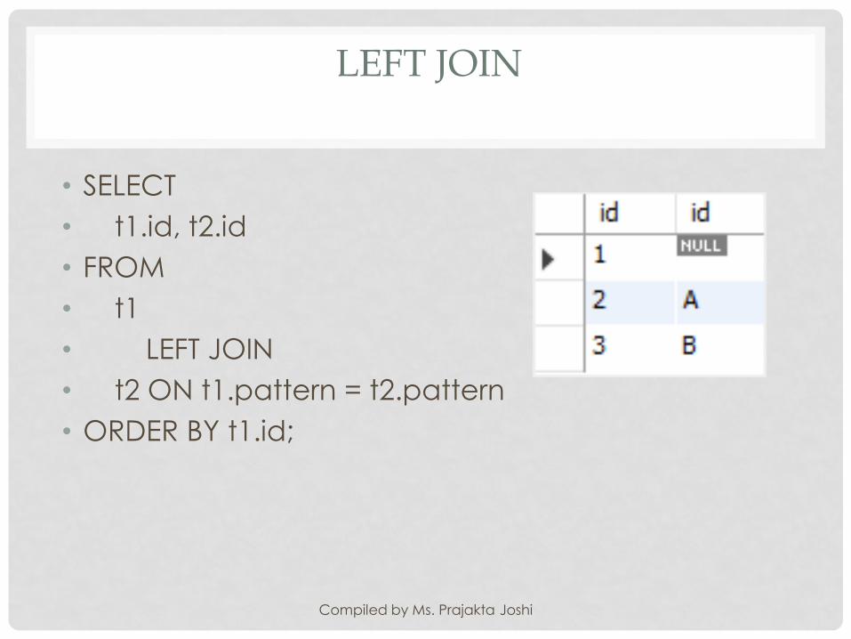
LEFT JOIN
• SELECT
• t1.id, t2.id
• FROM
• t1
• LEFT JOIN
• t2 ON t1.pattern = t2.pattern
• ORDER BY t1.id;
Compiled by Ms. Prajakta Joshi

RIGHT JOIN
• A RIGHT JOIN is similar to the LEFT JOIN except that the treatment of tables is reversed.
• With a RIGHT JOIN, every row from the right table ( t2) will appear in the result set.
• For the rows in the right table that do not have the matching rows in the left table ( t1), NULLs appear for columns in the left table ( t1).
Compiled by Ms. Prajakta Joshi

RIGHT JOIN
• SELECT
• t1.id, t2.id
• FROM
• t1
• RIGHT JOIN
• t2 on t1.pattern = t2.pattern
• ORDER BY t2.id;
Compiled by Ms. Prajakta Joshi

RELATIONAL CALCULAS
Compiled by Ms. Prajakta Joshi

TUPLE RELATIONAL CALCULUS
• In this form of relational calculus, we define a tuple variable, specify the table(relation) name in which the tuple is to be searched for, along with a condition.
• We can also specify column name using a . dot operator, with the tuple variable to only get a certain attribute(column) in result.
• A lot of information, right! Give it some time to sink in.
• A tuple variable is nothing but a name, can be anything, generally we use a single alphabet for this, so let's say T is a tuple variable.
Compiled by Ms. Prajakta Joshi
DOMAIN RELATIONAL CALCULUS (DRC)
• In domain relational calculus, filtering is done based on the domain of the attributes and not based on the tuple values.
• Syntax: { c1, c2, c3, ..., cn | F(c1, c2, c3, ... ,cn)}
• where, c1, c2... etc represents domain of attributes(columns) and F defines the formula including the condition for fetching the data.
Compiled by Ms. Prajakta Joshi
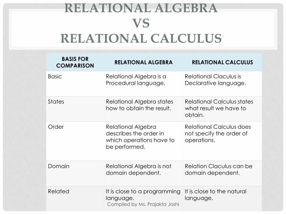
RELATIONAL ALGEBRAVS
RELATIONAL CALCULUS
BASIS FOR COMPARISON
RELATIONAL ALGEBRA RELATIONAL CALCULUS
Basic Relational Algebra is a Procedural language.
Relational Claculus is Declarative language.
States Relational Algebra states how to obtain the result.
Relational Calculus states what result we have to obtain.
Order Relational Algebra describes the order in which operations have to be performed.
Relational Calculus does not specify the order of operations.
Domain Relational Algebra is not domain dependent.
Relation Claculus can be domain dependent.
Related It is close to a programming language.
It is close to the natural language.
Compiled by Ms. Prajakta Joshi