


Languages
Pages
Legal

Entanglement negativity in a two dimensional
harmonic lattice: Area law and corner contributions
Cristiano De Nobili1, Andrea Coser2 and Erik Tonni1
1 SISSA and INFN, via Bonomea 265, 34136 Trieste, Italy.2 Departamento de Analisis Matematico, Universidad Complutense de Madrid, 28040
Madrid, Spain.
Abstract. We study the logarithmic negativity and the moments of the partial
transpose in the ground state of a two dimensional massless harmonic square lattice
with nearest neighbour interactions for various configurations of adjacent domains. At
leading order for large domains, the logarithmic negativity and the logarithm of the ratio
between the generic moment of the partial transpose and the moment of the reduced
density matrix at the same order satisfy an area law in terms of the length of the curve
shared by the adjacent regions. We give numerical evidences that the coefficient of
the area law term in these quantities is related to the coefficient of the area law term
in the Renyi entropies. Whenever the curve shared by the adjacent domains contains
vertices, a subleading logarithmic term occurs in these quantities and the numerical
values of the corner function for some pairs of angles are obtained. In the special case of
vertices corresponding to explementary angles, we provide numerical evidence that the
corner function of the logarithmic negativity is given by the corner function of the Renyi
entropy of order 1/2.
arX
iv:1
604.
0260
9v2
[co
nd-m
at.s
tat-
mec
h] 1
9 A
pr 2
017
Entanglement negativity in a two dimensional harmonic lattice 2
Contents
1 Introduction 2
2 Harmonic lattice 6
2.1 Hamiltonian and correlators . . . . . . . . . . . . . . . . . . . . . . . . . . 6
2.2 Entanglement entropies . . . . . . . . . . . . . . . . . . . . . . . . . . . . . 8
2.3 Moments of the partial transpose and logarithmic negativity . . . . . . . . 8
3 Area law 9
3.1 Logarithmic negativity . . . . . . . . . . . . . . . . . . . . . . . . . . . . . 9
3.2 Moments of the partial transpose . . . . . . . . . . . . . . . . . . . . . . . 13
4 Logarithmic term from the corner contributions 15
4.1 Entanglement entropies . . . . . . . . . . . . . . . . . . . . . . . . . . . . . 15
4.2 Logarithmic negativity . . . . . . . . . . . . . . . . . . . . . . . . . . . . . 17
4.3 Comments on the continuum limit . . . . . . . . . . . . . . . . . . . . . . . 22
5 Conclusions 25
1. Introduction
The entanglement in extended quantum systems and the ways to quantify it has attracted
a lot of research during the last decade in different areas of theoretical physics like
condensed matter, quantum information and quantum gravity (see [1] for reviews).
Given a quantum system in a pure state |Ψ〉 and assuming that its Hilbert space
is bipartite, i.e. H = HA ⊗ HB, the entanglement entropy is an important quantity to
measure the entanglement between the two parts of the system. In this manuscript we
consider only spatial bipartitions, denoting by A a generic spatial region and by B its
complement. The A’s reduced density matrix ρA is obtained by tracing over HB the
density matrix ρ = |Ψ〉〈Ψ| of the entire system. The normalisation condition is TrρA = 1
and the Von Neumann entropy of ρA defines the entanglement entropy, namely
SA = −Tr(ρA log ρA) . (1)
The entanglement entropy SB obtained from B’s reduced density matrix can be introduced
in the same way. When ρ is a pure state, we have that SB = SA.
Important quantities to study the bipartite entanglement of pure states are also the
Renyi entropies, which are defined as follows
S(n)A =
1
1− nlog TrρnA , (2)
where n > 2 is an integer parameter. The entanglement entropy (1) can be found from
the Renyi entropies (2) as SA = − limn→1 ∂nTrρnA = limn→1 S(n)A . This limit requires to
Entanglement negativity in a two dimensional harmonic lattice 3
perform an analytical continuation of S(n)A to real values of n close to n = 1. For a pure
state S(n)B = S
(n)A for any value of n.
When the subsystem A = A1∪A2 is made by two regions, which can be either disjoint
or adjacent, an interesting quantity to consider is the mutual information, i.e.
IA1,A2 = SA1 + SA2 − SA1∪A2 = limn→1
I(n)A1,A2
, (3)
where I(n)A1,A2
= S(n)A1
+ S(n)A2− S(n)
A1∪A2is the corresponding combination of Renyi entropies.
The mutual information measures the total amount of correlations between the two
systems [2, 3].
For some quantum systems on the lattice, the entanglement entropy SA grows like
the area of the boundary of the subsystem A as its size increases [4, 5]. This area law
behaviour of SA has been proved for gapped systems on the lattice [3], but for critical
systems the situation is more complicated: important exceptions are the critical systems
in one spatial dimension, where SA diverges logarithmically with the length of the interval
A [6], and free fermions in higher dimensions [7].
When the continuum limit is described by a quantum field theory, an ultraviolet
(UV) cutoff ε must be introduced and SA is a divergent quantity for ε→ 0. The area law
behaviour can occur in the coefficient of the most divergent term, which is non universal
and turns out to be proportional to the area of ∂A (i.e. the boundary of A) in these
cases. A quantum system in the continuum at criticality is described by a conformal field
theory (CFT). Considering a 1 + 1 dimensional CFT on a line at zero temperature and
an interval A of length `, we have that SA = (c/3) log(`/ε) + const, where c is the central
charge of the model [8]. Instead, the mutual information (3) of two disjoint intervals is
UV finite and it depends on the full operator content of the model [9]. Performing the
replica limit to get analytic expressions for SA and IA1,A2 from the ones for S(n)A and I
(n)A1,A2
can be a very difficult task (see [10, 11] for a numerical approach).
In 2 + 1 dimensional CFTs and for domains A whose boundary is smooth, the
expansion of the Renyi entropies reads S(n)A = αn PA/ε + const as ε → 0, where PA
is the perimeter of A and the coefficient αn depends on the model and on the details of
the UV regularisation. The replica limit implies that SA = α PA/ε+const as ε→ 0, where
limn→1 αn = α. When the two dimensional spatial domain A has a non smooth boundary,
S(n)A contains also a subleading logarithmic term whose coefficient is independent of the
regularisation details. Such coefficient is obtained as the sum of the contributions of
the vertices of the curve ∂A, where each term is given by a model dependent function
(corner function) evaluated on the opening angle in A of the corresponding vertex. Many
interesting studies have been done on such corner functions in various lattice models
[12, 13, 14, 15]. For a CFT in 2+1 dimensions, it has been recently found that the leading
term in the expansion of the corner function as the opening angle θ is close to π provides
the constant characterising the two-point function of the stress tensor [16, 17]. Within
the context of the AdS/CFT correspondence, the prescription to compute holographically
the entanglement entropy in the regime where classical gravity can be employed has been
Entanglement negativity in a two dimensional harmonic lattice 4
found in [18]. In the case of AdS4/CFT3, such holographic prescription provides also the
expected subleading logarithmic divergence whenever ∂A contains vertices [19].
The mutual information (3) of disjoint domains with smooth boundaries is a UV
finite quantity because the area law terms cancel. When the separation between the
regions is large with respect to their sizes, analytic results have been found [20]. In the
case of two dimensional adjacent domains A1 and A2, both the mutual information and its
generalisation involving the Renyi entropies display an area law behaviour in terms of the
length of the curve shared by the adjacent regions. In particular, I(n)A1,A2
= 2αnPshared/ε+. . .
and IA1,A2 = 2α Pshared/ε+ . . . as ε→ 0, where Pshared ≡ length(∂A1 ∩ ∂A2).
The entanglement entropy and the Renyi entropies are measures of the quantum
entanglement for a bipartite system in a pure state, but this is not true when the whole
system is in a mixed state. For instance, the mutual information of a bipartite system
in a thermal state is dominated by classical correlations. Another important example of
mixed state is the reduced density matrix ρA associated to a subsystem A, when the entire
system is in its ground state. Splitting A in two domains A1 and A2, which can be either
adjacent or disjoint, it is worth considering the bipartite entanglement between them.
Many measures of the bipartite entanglement for a mixed state have been proposed in
quantum information theory, but they are usually very difficult to compute, even for small
systems. A measure which is computable also for extended systems is the logarithmic
negativity [21].
Let us consider a mixed state characterised by the density matrix ρ acting on a
spatially bipartite Hilbert space H = HA1 ⊗ HA2 . We remark that H can be either the
Hilbert space characterising the whole spatial system or the one HA associated to the
bipartite subsystem A = A1 ∪ A2 introduced above (in the latter case ρ = ρA). The
logarithmic negativity is defined through the partial transpose of ρ with respect to one of
the two parts. Considering e.g. the partial transposition with respect to A2, the matrix
element of ρT2 is given by
〈e(1)i e(2)j |ρT2|e
(1)k e
(2)l 〉 = 〈e(1)i e
(2)l | ρ |e
(1)k e
(2)j 〉 . (4)
Since the spectrum of the Hermitian matrix ρT2 can contain also negative eigenvalues, it
is worth computing its trace norm ‖ρT2A ‖ = Tr|ρT2| =∑
i |λi|. The logarithmic negativity
is defined as
E ≡ log Tr|ρT2| . (5)
The logarithmic negativity can be computed also by employing a replica limit [22, 23].
Considering the n-th moment Tr(ρT2)n of the partial transpose and taking into account
only the sequence of the even powers n = ne, it is not difficult to realise that (5) can be
found by performing the following analytic continuation
E = limne→1
log Tr(ρT2)ne. (6)
In the special case of a pure state ρ = |Ψ〉〈Ψ| acting on a bipartite Hilbert space, the
Entanglement negativity in a two dimensional harmonic lattice 5
moments of the partial transpose are related to the Renyi entropies as follows [22, 23]
Tr(|Ψ〉〈Ψ|T2
)n=
{Trρno
A2odd n = no ,(
Trρne/2A2
)2even n = ne ,
(7)
where ρA2 = TrA1|Ψ〉〈Ψ| is the reduced density matrix of the subsystem A2. From the
relation (7) and the replica limit (6), one easily gets that E = S(1/2)A2
.
The logarithmic negativity and the moments Tr(ρT2A )n of the partial transpose are
interesting quantities to compute for bipartite mixed states. In this manuscript we focus
on a particular system in its ground state, considering the mixed state given by the
reduced density matrix ρA = TrHB|Ψ〉〈Ψ| of a spatial subsystem, whose corresponding
Hilbert space HA = HA1 ⊗HA2 is bipartite. Instead of the moments of ρT2A , we find more
convenient to consider the following quantity
En ≡ log
(Tr(ρT2A )n
TrρnA
). (8)
It is not difficult to show that E2 = 0. Given the normalization condition of ρA, the replica
limit (6) tells that
E = limne→1Ene . (9)
For 1 + 1 dimensional CFTs in the ground state, the logarithmic negativity and
the moments of the partial transpose have been studied for both adjacent and disjoint
intervals [22, 23, 24]. This analysis has been extended also to a bipartite system at
finite temperature [25]. The moments of the partial transpose for some fermionic systems
on the lattice have been studied through a method involving correlators in [26, 27] and
the overlap matrix in [28]. The logarithmic negativity has been considered also for a
non vanishing mass [23, 29] and out of equilibrium [30, 31]. Other interesting numerical
studies for various one dimensional lattice systems have been performed in [32]. The same
numerical method employed to get the mutual information from the replica limit has been
used to get the logarithmic negativity from the replica limit (6), since similar difficulties
occur [11].
In two spatial dimensions, the logarithmic negativity of topological systems has been
considered [33] and recently interesting lattice analysis have been performed for both
fermionic and bosonic systems [34, 35]. Some results have been found also in the context
of holography [36].
In this paper we consider a two dimensional square harmonic lattice with nearest
neighbour interactions in its ground state. We focus on the regime of massless oscillators,
whose continuum limit is described by the CFT given by the massless scalar field in
2 + 1 dimensions. In the thermodynamic limit, we study the logarithmic negativity and
the quantity (8) for various configurations of adjacent domains in the regime where they
become large. At leading order, these quantities follow an area law behaviour in terms of
the length of the curve shared by the adjacent regions. This observation for the logarithmic
negativity has been already done for this model in [34], where the configuration given by
Entanglement negativity in a two dimensional harmonic lattice 6
two halves of a square has been considered. We notice that the coefficient of the area law
term is related to the coefficient of the area law term in the Renyi entropies. We study
also the subleading logarithmic term, which occurs whenever the curve shared by the
adjacent regions contains vertices. Such term is very interesting because it is independent
of the regularisation details.
The layout of this manuscript is as follows. In §2 we review the method to compute
SA, S(n)A , E and En for this bosonic lattice. In §3 we investigate the area law behaviour in
the leading term of E and En for various configurations of large adjacent domains in the
infinitely extended lattice. In §4 we study the subleading logarithmic term of E due to
the occurrence of vertices in the curve shared by the adjacent domains and in §5 we draw
some conclusions.
2. Harmonic lattice
In this section we introduce the lattice model considered throughout this manuscript,
its correlators in the thermodynamic limit and their role in computing the entanglement
entropies, the moments of the partial transpose and the logarithmic negativity.
2.1. Hamiltonian and correlators
We consider the two dimensional square lattice made by harmonic oscillators coupled
through the nearest neighbour spring-like interaction. Denoting by Lx and Ly the number
of sites (oscillators) along the two orthogonal directions, such lattice contains N = LxLyoscillators. The Hamiltonian of the model reads
H =∑
16i6Lx16j6Ly
{p2i,j2M
+Mω2
2q2i,j +
K
2
[(qi+1,j − qi,j
)2+(qi,j+1 − qi,j
)2]}, (10)
where the pair of integers (i, j) identifies a specific lattice site. The canonical variables
qi,j and pi,j satisfy the canonical commutation relation [qi,j, qr,s] = [pi,j, pr,s] = 0 and
[qi,j, pr,s] = i δi,rδj,s. We assume periodic boundary conditions along both the spatial
directions, namely qLx+k,j = qk,j, pLx+k,j = pk,j, qj,Ly+k = qj,k and pj,Ly+k = pj,k for a
generic integer k.
The model described by (10) contains three parameters ω, M and K, but not all
of them are independent. Indeed, by performing the canonical rescaling (qi,j, pi,j) →( 4√MKqi,j, pi,j/
4√MK) and introducing a =
√M/K, the Hamiltonian (10) becomes
H =∑
16i6Lx16j6Ly
{p2i,j2a
+aω2
2q2i,j +
1
2a
[(qi+1,j − qi,j
)2+(qi,j+1 − qi,j
)2]}. (11)
From this expression, one can easily observe that (10) gives the Hamiltonian of a free scalar
field with mass ω in two spatial dimensions discretised on a square lattice with lattice
spacing a. The continuum limit corresponds to take simultaneously the limits Lx → ∞,
Entanglement negativity in a two dimensional harmonic lattice 7
Ly → ∞ and a → 0, while Lxa and Lya are kept fixed. In our lattice computations,
without loss of generality, we set K = M = 1. The Hamiltonian (10) can be diagonalised
in a standard way, finding the following dispersion relation
ωk ≡√ω2 + 4
[sin2(πkx/Lx) + sin2(πky/Ly)
]> ω , (12)
where k = (kx, ky) is a pair of integers such that 0 6 kx < Lx and 0 6 ky < Ly. Because
of the translation invariance of the model, the zero mode with k = (0, 0) occurs, for which
the equality holds in (12).
In our analysis we need the following vacuum correlators
〈0|qi,jqr,s|0〉 =1
2LxLy
∑06kx<Lx06ky<Ly
1
ωk
cos[2πkx(i− r)/Lx] cos[2πky(j − s)/Ly] , (13)
〈0|pi,jpr,s|0〉 =1
2LxLy
∑06kx<Lx06ky<Ly
ωk cos[2πkx(i− r)/Lx] cos[2πky(j − s)/Ly] , (14)
which are the matrix elements of the correlation matrices Q and P respectively (where (i, j)
and (r, s) are the raw and column indices respectively). These matrices satisfy Q·P = I/4,
being I is the identity matrix. We remark that the term in (13) corresponding to the zero
mode reads 1/(2LxLyω), which is divergent for ω → 0. This implies that we cannot take
ω = 0 in a finite lattice.
Since from our computations on the lattice we would like to extract information
about the model in the continuum limit, we need to consider the regime where Lx, Ly �` � 1, being ` the linear size of the subsystem. Thus, it is convenient to consider the
thermodynamic limit, where Lx → ∞ and Ly → ∞, while the lattice spacing a is kept
finite. In order to perform the thermodynamic limit of the correlators (13) and (14), we
define qr = 2πkr/Lr for r ∈ {x, y}. In the thermodynamic limit qr becomes a continuous
variable qr ∈ [0, 2π) and the sum in (13) and (14) is replaced by an integration according
to 1Lr
∑kr→∫ 2π
0dqr2π
. Thus, the correlators (13) and (14) in the thermodynamic limit
become respectively
〈0|qi,jqr,s|0〉 =1
8π2
∫ 2π
0
1
ωq
cos[qx(i− r)] cos[qy(j − s)] dqxdqy , (15)
〈0|pi,jpr,s|0〉 =1
8π2
∫ 2π
0
ωq cos[qx(i− r)] cos[qy(j − s)] dqxdqy , (16)
where ωq =√ω2 + 4[sin2(qx/2) + sin2(qy/2)], with q = (qx, qy). When ω = 0 the integral
in (15) is convergent and therefore, in principle, the massless regime can be considered
without any approximation. Nevertheless, in order to avoid divergent integrands, in our
numerical calculations we have set ω 6 10−6, checking in some cases that smaller values
of ω do not lead to significant changes in the final result.
Entanglement negativity in a two dimensional harmonic lattice 8
2.2. Entanglement entropies
Following [37], we can compute the Renyi entropies S(n)A for this model by considering
the matrices QA and PA, which are obtained by restricting Q and P respectively to the
subsystem A. Their size is NA × NA, being NA the number of lattice points inside the
region A.
The matrix product QA · PA has positive eigenvalues {µ21, . . . , µ
2NA} with µ2
i > 1/4
and the moments of the reduced density matrix are given by
TrρnA =
NA∏j=1
[(µj +
1
2
)n−(µj −
1
2
)n ]−1. (17)
From this expression it is straightforward to get the Renyi entropies
S(n)A =
1
1− nlog TrρnA =
1
n− 1
NA∑j=1
log
[(µj +
1
2
)n−(µj −
1
2
)n ], (18)
while the entanglement entropy is given by
SA =
NA∑j=1
[(µj +
1
2
)log
(µj +
1
2
)−(µj −
1
2
)log
(µj −
1
2
)]. (19)
By employing these formulas for disjoint domains on the lattice, one gets I(n)A1,A2
and
the mutual information IA1,A2 .
2.3. Moments of the partial transpose and logarithmic negativity
In [38] it was shown that the partial transposition with respect to A2 for a bosonic state
corresponds to the time reversal applied only to the degrees of freedom in A2, while
the remaining ones are untouched. In particular, in A2 the positions are left invariant
qi,j → qi,j everywhere, while the momenta are reversed pi,j → −pi,j if (i, j) ∈ A2. Given a
bosonic Gaussian state, like the ground state of the harmonic chain we are considering,
the resulting operator after such transformation will be Gaussian as well. It is worth
remarking that this is not true for fermionic systems. For instance, for free fermions
the partial transpose of the ground state density matrix can be written as a sum of two
Gaussian operators [26].
The above observations are implemented on our lattice model by introducing the
following matrix
PT2A = RA2 · PA · RA2 , (20)
where RA2 is the NA × NA diagonal matrix having −1 in correspondence of the sites
belonging to A2 and +1 otherwise. Since RA1 = −RA2 , it is easy to observe that PT1A = PT2A ,
as expected. The matrix QA · PT2A has also positive eigenvalues {ν21 , . . . , ν2NA}, but if the
state is entangled some of them can be smaller than 1/4. From the eigenvalues νj one
Entanglement negativity in a two dimensional harmonic lattice 9
gets the moments of the partial transpose of the reduced density matrix as in (17) for the
moments of the reduced density matrix, namely
Tr(ρT2A)n
=
NA∏j=1
[(νj +
1
2
)n−(νj −
1
2
)n ]−1. (21)
The trace norm of ρT2A reads
∥∥ρT2A ∥∥ =
NA∏j=1
[ ∣∣∣∣νj +1
2
∣∣∣∣− ∣∣∣∣νj − 1
2
∣∣∣∣ ]−1 =
NA∏j=1
max
(1,
1
2νj
), (22)
which leads straightforwardly to the logarithmic negativity
E =
NA∑j=1
log[max
(1, (2νj)
−1)] . (23)
In the remaining part of the manuscript we discuss the numerical results obtained
by employing the above lattice formulas.
3. Area law
In this section we consider various configurations of adjacent domains for the harmonic
lattice in the thermodynamic limit described in §2. For large domains, we show that at
leading order the logarithmic negativity and En satisfy an area law in terms of the length
of the curve shared by the adjacent domains. We observe that the coefficient of such term
in these quantities is related to the coefficient of the area law term in the Renyi entropies.
3.1. Logarithmic negativity
We begin our analysis by considering the logarithmic negativity of two equal adjacent
rectangles A1 and A2 which share an edge along the vertical y axis, as shown in the inset
of the left panel in Fig. 1, where the adjacent domains are highlighted by blue dots and red
circles. These rectangles have the natural orientation induced by the underlying lattice,
namely their edges are parallel to the vectors generating the square lattice. Denoting by
`x and `y the lengths of the edges along the x and y directions respectively, the numerical
data for E of this configuration of adjacent domains are plotted in Fig. 1.
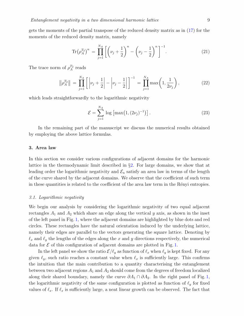
In the left panel we show the ratio E/`y as function of `x when `y is kept fixed. For any
given `y, such ratio reaches a constant value when `x is sufficiently large. This confirms
the intuition that the main contribution to a quantity characterising the entanglement
between two adjacent regions A1 and A2 should come from the degrees of freedom localized
along their shared boundary, namely the curve ∂A1 ∩ ∂A2. In the right panel of Fig. 1,
the logarithmic negativity of the same configuration is plotted as function of `y for fixed
values of `x. If `x is sufficiently large, a neat linear growth can be observed. The fact that
Entanglement negativity in a two dimensional harmonic lattice 10
Figure 1. Area law behaviour for the logarithmic negativity E between two equal
rectangles, whose edges have lengths `x and `y, which are adjacent along the vertical edge
(inset of the left panel). Left: For fixed values of `y, the ratio E/`y reaches a constant
value as `x increases. Right: For fixed and large enough values of `x, the logarithmic
negativity grows linearly as `y increases (the dashed line is obtained by fitting all the
data corresponding to `x = 11).
the asymptotic value of E/`y depends on `y in the left panel of Fig. 1 is mainly due to the
subleading corner contributions, which will be largely discussed in §4.
These results tell us that, given two equal and large enough adjacent regions A1 and
A2, at leading order the logarithmic negativity E between them increases like the length
of the curve ∂A1 ∩ ∂A2 shared by their boundaries as their size increases. Such length
will be denoted by Pshared ≡ length(∂A1 ∩ ∂A2) throughout this manuscript. Thus, the
logarithmic negativity between large adjacent domains satisfies an area law in terms of
the region shared by their boundaries. This observation has been recently done for this
model also by Eisler and Zimboras [34], who have considered the logarithmic negativity
between the two halves of a square as the length of its edge increases.
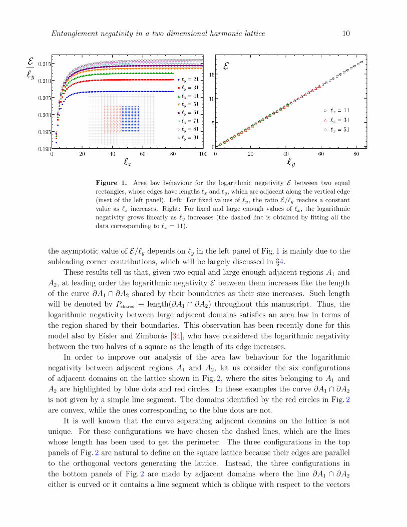
In order to improve our analysis of the area law behaviour for the logarithmic
negativity between adjacent regions A1 and A2, let us consider the six configurations
of adjacent domains on the lattice shown in Fig. 2, where the sites belonging to A1 and
A2 are highlighted by blue dots and red circles. In these examples the curve ∂A1 ∩ ∂A2
is not given by a simple line segment. The domains identified by the red circles in Fig. 2
are convex, while the ones corresponding to the blue dots are not.
It is well known that the curve separating adjacent domains on the lattice is not
unique. For these configurations we have chosen the dashed lines, which are the lines
whose length has been used to get the perimeter. The three configurations in the top
panels of Fig. 2 are natural to define on the square lattice because their edges are parallel
to the orthogonal vectors generating the lattice. Instead, the three configurations in
the bottom panels of Fig. 2 are made by adjacent domains where the line ∂A1 ∩ ∂A2
either is curved or it contains a line segment which is oblique with respect to the vectors
Entanglement negativity in a two dimensional harmonic lattice 11
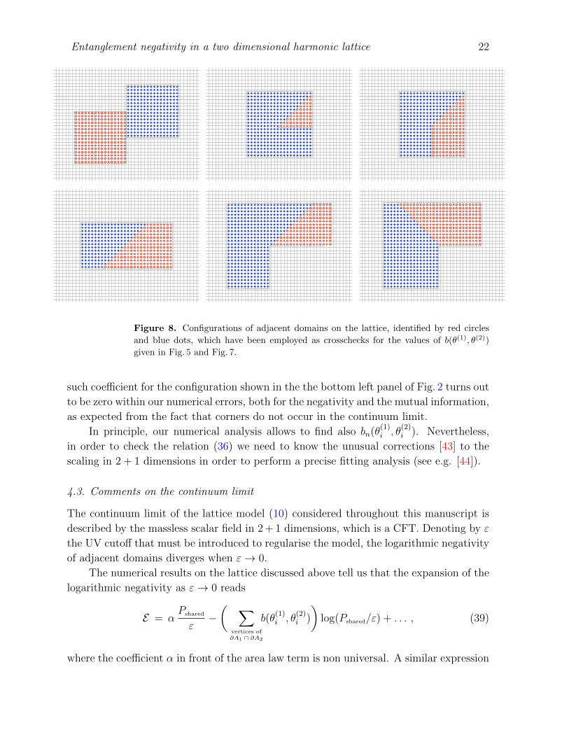
Figure 2. Configurations of adjacent domains on the lattice, identified by red circles
and blue dots, which have been employed to study the area law behaviour (see §3 and
Figs. 3 and 4) and the corner contributions for explementary angles (see §4 and Fig. 5).
generating the lattice. Notice that a disk of given radius on the lattice could include a
different number of sites depending on whether the centre of the disk is located on a lattice
site or within a plaquette. Such ambiguity does not affect the leading order behaviour
of the quantities that we are considering, but it could be relevant for subleading terms
[14, 39].
Also for the logarithmic negativity of the adjacent domains shown in Fig. 2 we have
observed the same qualitative behaviour described in the left panel of Fig. 1 for the equal
adjacent rectangles: by keeping fixed the region corresponding to the red circles while the
sizes of the region characterised by the blue dots increase, E saturates to a constant value.
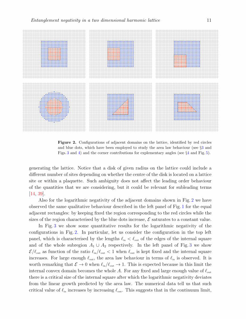
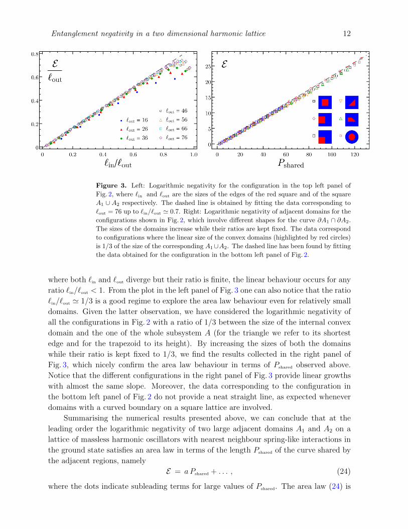
In Fig. 3 we show some quantitative results for the logarithmic negativity of the
configurations in Fig. 2. In particular, let us consider the configuration in the top left
panel, which is characterised by the lengths `in < `out of the edges of the internal square
and of the whole subregion A1 ∪ A2 respectively. In the left panel of Fig. 3 we show
E/`out as function of the ratio `in/`out < 1 when `out is kept fixed and the internal square
increases. For large enough `out, the area law behaviour in terms of `in is observed. It is
worth remarking that E → 0 when `in/`out → 1. This is expected because in this limit the
internal convex domain becomes the whole A. For any fixed and large enough value of `outthere is a critical size of the internal square after which the logarithmic negativity deviates
from the linear growth predicted by the area law. The numerical data tell us that such
critical value of `in increases by increasing `out. This suggests that in the continuum limit,
Entanglement negativity in a two dimensional harmonic lattice 12
Figure 3. Left: Logarithmic negativity for the configuration in the top left panel of
Fig. 2, where `in and `out are the sizes of the edges of the red square and of the square
A1 ∪ A2 respectively. The dashed line is obtained by fitting the data corresponding to
`out = 76 up to `in/`out ' 0.7. Right: Logarithmic negativity of adjacent domains for the
configurations shown in Fig. 2, which involve different shapes for the curve ∂A1 ∩ ∂A2.
The sizes of the domains increase while their ratios are kept fixed. The data correspond
to configurations where the linear size of the convex domains (highlighted by red circles)
is 1/3 of the size of the corresponding A1∪A2. The dashed line has been found by fitting
the data obtained for the configuration in the bottom left panel of Fig. 2.
where both `in and `out diverge but their ratio is finite, the linear behaviour occurs for any
ratio `in/`out < 1. From the plot in the left panel of Fig. 3 one can also notice that the ratio
`in/`out ' 1/3 is a good regime to explore the area law behaviour even for relatively small
domains. Given the latter observation, we have considered the logarithmic negativity of
all the configurations in Fig. 2 with a ratio of 1/3 between the size of the internal convex
domain and the one of the whole subsystem A (for the triangle we refer to its shortest
edge and for the trapezoid to its height). By increasing the sizes of both the domains
while their ratio is kept fixed to 1/3, we find the results collected in the right panel of
Fig. 3, which nicely confirm the area law behaviour in terms of Pshared observed above.
Notice that the different configurations in the right panel of Fig. 3 provide linear growths
with almost the same slope. Moreover, the data corresponding to the configuration in
the bottom left panel of Fig. 2 do not provide a neat straight line, as expected whenever
domains with a curved boundary on a square lattice are involved.
Summarising the numerical results presented above, we can conclude that at the
leading order the logarithmic negativity of two large adjacent domains A1 and A2 on a
lattice of massless harmonic oscillators with nearest neighbour spring-like interactions in
the ground state satisfies an area law in terms of the length Pshared of the curve shared by
the adjacent regions, namely
E = aPshared + . . . , (24)
where the dots indicate subleading terms for large values of Pshared. The area law (24) is
Entanglement negativity in a two dimensional harmonic lattice 13
consistent with the fact that E measures the bipartite entanglement between A1 and A2
for the mixed state characterised by the reduced density matrix ρA1∪A2 . The coefficient a
in (24) is non universal, i.e. it depends on the ultraviolet details.
Given the two adjacent regions A1 and A2 considered above, another very interesting
quantity to study is their mutual information IA1,A2 , which has been defined in (3). Since
the area law of the entanglement entropy for large domains tells us that SA = a PA + . . . ,
it is straightforward to find that IA1,A2 of adjacent domains satisfies an area law in terms
of Pshared. In particular, we have that
IA1,A2 = 2a Pshared + . . . , (25)
where, as above, the dots stand for subleading terms.
3.2. Moments of the partial transpose
The moments Tr(ρT2A )n of the partial transpose for integer values of n are interesting
quantities to study because they provide the logarithmic negativity through the replica
limit (6) [22, 23].
Given the configurations of adjacent domains described in §3.1, instead of considering
the n-th moment of the partial transpose, we find it more interesting the ratio En defined
in (8), which also provides the logarithmic negativity through the replica limit (9) because
of the normalisation condition TrρA = 1. In our model, the main reason to consider Eninstead of log Tr(ρT2)n occurring in (6) is that, by repeating the analysis described in §3.1,
we find that, at leading order for large adjacent domains, En follows an area law in terms
of the length of the curve shared by the adjacent domains, i.e.
En = an Pshared + . . . , (26)
where the non universal coefficient an depends on the integer n and the dots denote
subleading terms. We recall that the Renyi entropies of our model satisfy the area law
S(n)A = an PA + . . . , where the coefficient an is non universal as well and limn→1 an = a.
From (26) and the area law of the Renyi entropies it is straightforward to find the
leading term of the logarithm of the moments of the partial transpose, which is given by
log Tr(ρT2A)n
= an Pshared + (1− n)an PA + . . . . (27)
Thus, the quantities log Tr(ρT2A )n contain an area law contribution also from the boundary
of A = A1 ∪ A2. Since limne→1(ne − 1)ane = 0, such term cancels in the replica limit
(6). A similar cancellation occurs also for adjacent intervals in 1 + 1 dimensional CFTs.
Indeed, considering the divergent terms for ε→ 0, in En only the ones giving a non trivial
contribution after the replica limit survive, while log Tr(ρT2)n contains also other terms
[23], which vanish in the replica limit (6). The quantity En for adjacent intervals in 1 + 1
dimensional CFTs has been studied in [25, 30] and for free fermions on a two dimensional
lattice in [34].
Entanglement negativity in a two dimensional harmonic lattice 14
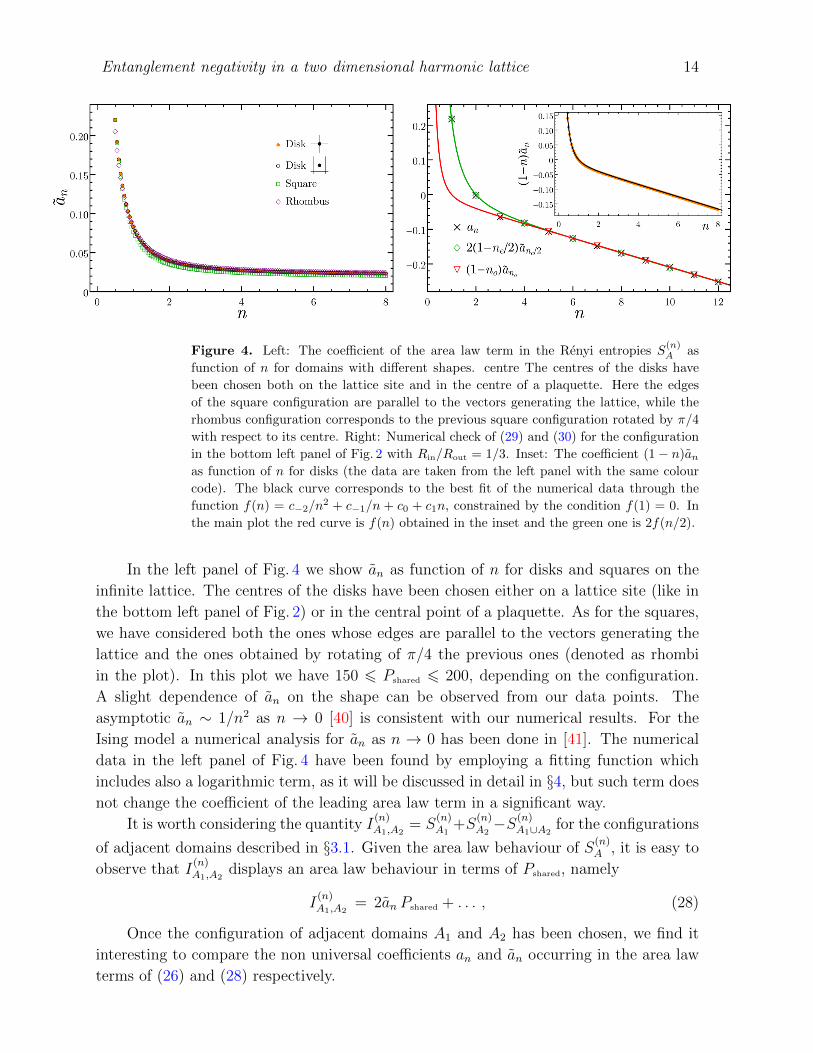
Figure 4. Left: The coefficient of the area law term in the Renyi entropies S(n)A as
function of n for domains with different shapes. centre The centres of the disks have
been chosen both on the lattice site and in the centre of a plaquette. Here the edges
of the square configuration are parallel to the vectors generating the lattice, while the
rhombus configuration corresponds to the previous square configuration rotated by π/4
with respect to its centre. Right: Numerical check of (29) and (30) for the configuration
in the bottom left panel of Fig. 2 with Rin/Rout = 1/3. Inset: The coefficient (1− n)anas function of n for disks (the data are taken from the left panel with the same colour
code). The black curve corresponds to the best fit of the numerical data through the
function f(n) = c−2/n2 + c−1/n + c0 + c1n, constrained by the condition f(1) = 0. In
the main plot the red curve is f(n) obtained in the inset and the green one is 2f(n/2).
In the left panel of Fig. 4 we show an as function of n for disks and squares on the
infinite lattice. The centres of the disks have been chosen either on a lattice site (like in
the bottom left panel of Fig. 2) or in the central point of a plaquette. As for the squares,
we have considered both the ones whose edges are parallel to the vectors generating the
lattice and the ones obtained by rotating of π/4 the previous ones (denoted as rhombi
in the plot). In this plot we have 150 6 Pshared 6 200, depending on the configuration.
A slight dependence of an on the shape can be observed from our data points. The
asymptotic an ∼ 1/n2 as n → 0 [40] is consistent with our numerical results. For the
Ising model a numerical analysis for an as n → 0 has been done in [41]. The numerical
data in the left panel of Fig. 4 have been found by employing a fitting function which
includes also a logarithmic term, as it will be discussed in detail in §4, but such term does
not change the coefficient of the leading area law term in a significant way.
It is worth considering the quantity I(n)A1,A2
= S(n)A1
+S(n)A2−S(n)
A1∪A2for the configurations
of adjacent domains described in §3.1. Given the area law behaviour of S(n)A , it is easy to
observe that I(n)A1,A2
displays an area law behaviour in terms of Pshared, namely
I(n)A1,A2
= 2an Pshared + . . . , (28)
Once the configuration of adjacent domains A1 and A2 has been chosen, we find it
interesting to compare the non universal coefficients an and an occurring in the area law
terms of (26) and (28) respectively.
Entanglement negativity in a two dimensional harmonic lattice 15
It is reasonable to expect that the area law term for En comes from effects localised
in the neighbourhood of the curve ∂A1 ∩ ∂A2. Thus, considering e.g. the configurations
in Fig. 2 where the domain identified by the red circles is entirely surrounded by the one
characterised by the blue dots (i.e. the configurations in the top left, bottom middle and
bottom right panels), such term should be independent of the size of the domain identified
by the blue dots. In the limit where this domain becomes the whole region complementary
to the one identified by the red circles, one gets the bipartition of the ground state. These
considerations suggest us that an in (26) is the same one occurring for a bipartition of
the ground state, when the identity (7) can be applied. This implies that the following
relation should hold
an =
{ (1− no
)ano odd n = no ,
2(1− ne/2
)ane/2 even n = ne .
(29)
Notice that a2 = 0, as expected. By employing the relation (29) and the replica limit
(9), it is straightforward to find that the coefficient of the area law term in the logarithmic
negativity in (24) is equal to the coefficient of the area law term in the Renyi entropy of
order 1/2, namely
a = a1/2 . (30)
In the right panel of Fig. 4 we show a numerical check of the relations (29) and (30)
for the configuration in the bottom left panel of Fig. 2. In particular, the coincidence of
the data points corresponding to n = 1/2 provides a check of (30). The solid curve in the
inset is obtained by fitting the data with the function f(n) = c−2/n2 + c−1/n+ c0 + c1n,
where the parameters are constrained by the requirement that f(1) = 0. Thus, such fit
has three independent parameters. As for the solid curves in the main plot, the red one
is f(n), namely the black curve found in the inset, while the green one is 2f(n/2).
This analysis has been performed also for other configurations as further checks of
(29) and (30), finding the same qualitative behaviours.
4. Logarithmic term from the corner contributions
In this section we consider the subleading logarithmic term in E and En for adjacent
domains, which occurs whenever the shared curve ∂A1 ∩ ∂A2 contains some vertices,
where its endpoints are included among them. For vertices corresponding to explementary
angles, we provide some numerical evidence that the corner function of E is given by the
corner function of the Renyi entropy of order 1/2.
4.1. Entanglement entropies
Let us consider the entanglement entropy SA of a connected domain A whose boundary
contains some vertices (see Figs. 2, 6 and 8 for examples). For large size of A, the leading
term gives the area law behaviour. The occurrence of vertices in ∂A provides a subleading
Entanglement negativity in a two dimensional harmonic lattice 16
logarithmic term which is characterised by a corner function b(θ) as follows [12, 13, 14]
SA = a PA −( ∑
verticesof ∂A
b(θi)
)logPA + . . . 0 < θi 6 π , (31)
where θi is the opening angle in A corresponding to the i-th vertex of ∂A and the dots
denote subleading terms.
Since the logarithmic term is due to the corners, we have that b(π) = 0. From the
general property that SA = SB for pure states and a bipartite Hilbert spaceH = HA⊗HB,
we have that b(θ) = b(2π−θ), which tells us that b(θ) is defined for 0 < θ 6 π. The model
dependent corner function b(θ) is universal, i.e. independent of the ultraviolet details of
the regularisation. In the continuum limit, which is described by a 2+1 dimensional CFT,
the corner function b(θ) contains important information about the model. For instance,
recently it has been found that the constant σ entering in the asymptotic behaviour
b(θ) = σ(π−θ)2+. . . as θ → π at the leading order is related to the constant characterising
the correlator 〈Tµν(x)Tαβ(y)〉 of the underlying CFT [16]. The corner function b(θ) for the
massless scalar has been studied by Casini and Huerta [12]. In the context of holography,
by employing the prescription of [18] for SA, the corner function b(θ) has been studied
e.g. in [19].
We find it worth considering the mutual information (3) of two adjacent domains
A1 and A2 when their boundaries contain some vertices. For the sake of simplicity, we
focus on configurations such that either two or three curves meet at every vertex. Explicit
examples are shown in Figs. 2, 6 and 8, where the adjacent domains are identified by blue
dots and red circles. In the scaling limit, when their sizes increase while the ratios among
them are kept fixed, from (31) one finds that
IA1,A2 = 2a Pshared −( ∑
vertices of∂A1 ∩ ∂A2
[b(θ
(1)i ) + b(θ
(2)i )− b(θ(1∪2)i )
])log `+ . . . , (32)
where ` is a parameter characterising the common size of the adjacent regions, θ(k)i is the
angle in Ak and θ(1∪2)i the angle in A1 ∪A2 corresponding to the i-th vertex belonging to
∂A1 ∩ ∂A2. In the simplest case where such vertex is not an endpoint of ∂A1 ∩ ∂A2, it
provides a bipartition of the angle of 2π and the corresponding contribution to the sum
in (32) is 2b(θ(1)i ) = 2b(θ
(2)i ).
We find it instructive to consider explicitly the examples in Figs. 2 and 6. For the
configurations shown in the top left, middle and right panel of Fig. 2, the sum within
the parenthesis multiplying the logarithmic term in (32) is given by 8b(π/2), 8b(π/2) and
6b(π/2) respectively, while for the bottom middle and right panels of the same figure
it reads 4b(π/4) + 2b(π/2) and 2b(π/4) + 4b(π/2) + 2b(3π/4) respectively. As for the
configurations of Fig. 6, such coefficient is 4b(π/4)− 2b(π/2), 3b(π/4) + b(3π/4)− b(π/2)
and 4b(π/2) for the top left, middle and right panels respectively, while it is given by
3b(π/4) + b(3π/4) − 2b(π/2), 2b(π/2) and 2b(π/4) + 2b(3π/4) − 2b(π/2) for the bottom
left, middle and right panels respectively. It is not difficult to get the coefficient of the
Entanglement negativity in a two dimensional harmonic lattice 17
logarithmic term also for the configurations in Fig. 8. Let us point out that for the one in
the top left panel such coefficient is vanishing.
As for the Renyi entropies of domains with non smooth boundary, we have that
S(n)A = an PA −
( ∑verticesof ∂A
bn(θi)
)logPA + . . . , (33)
where the corner function bn(θ) depends on the order n and it provides b(θ) through the
replica limit, i.e. limn→1 bn(θi) = b(θi). For the model we are dealing with, the corner
function bn(θ) has been found in [12]. A formula similar to (32) can be written for I(n)A1,A2
,
by just replacing a with an and b(θ) with bn(θ).
4.2. Logarithmic negativity
Considering the scaling limit for the configurations of adjacent domains A1 and A2 in
Figs. 2, 6 and 8 where ∂A1 and ∂A2 contain vertices, the expansion of the logarithmic
negativity contains a subleading logarithmic term after the leading area law term. By
analogy with the case of the entanglement entropy, it is reasonable to expect that the
coefficient of the logarithmic term is obtained by summing the contributions of the vertices
occurring in ∂A1 and ∂A2. Extracting the coefficient of such subleading logarithmic term
from the lattice numerical data is a delicate task.
Let us first discuss the method employed to get the numerical values presented in
this section from the formulas discussed in §2. A first rough approach could consist
in fitting the numerical data by a linear term, a logarithmic term and a constant
one. Nevertheless, since the logarithmic contribution is tiny with respect to the linear
one, its estimation can be spoiled by the occurrence of subleading lattice effects. In
order to take them into account, we have inserted in our fitting analysis also some
standard power law corrections, i.e. we have fitted our data with a function of the form
c1`+ clog log(`) + c0 + c−1`−1 + · · ·+ c−kmax`
−kmax [12, 14], where ` is a characteristic length
of Pshared. In particular, considering the domains identified by red circles in Figs. 2, 6 and
8, in each configuration ` corresponds to the edge for squares, to the shortest edge for
the triangles, to the radius for the disks and to the height for the trapezoids. For each
data set, in the plots we show the results of various fits performed in different ranges of `,
where each range is specified by the starting value `start and by the ending value `end. We
fix some maximum exponent kmax and some `start by removing some initial points, which
are strongly affected by lattice effects and therefore would need more corrections. Then,
we plot the logarithmic coefficient obtained from different fits as a function of `end. The
parameters kmax, `start and the maximum value of `end are chosen in order to get a stable
result from the fits in the whole range of `end. The logarithmic coefficient is estimated as
the average of the fitted values within such range of `end. The error introduced through
this procedure is estimated by taking the maximum deviation of the data from the average
within this range of stability.
Entanglement negativity in a two dimensional harmonic lattice 18
An important benchmark employed to test our numerical analysis is the mutual
information of adjacent domains. In particular, we have considered the coefficient of the
logarithmic term in the mutual information for the configurations in the top left, bottom
middle and bottom right panels of Fig. 2, recovering the values of the corner function b(θ)
for θ ∈ {π/4, π/2, 3π/4} available in the literature [12, 14, 42].
Let us consider the occurrence of a subleading logarithmic term due to corners in the
logarithmic negativity of some configurations of adjacent domains. We first observe that
the angles of A1 and A2 contributing to the logarithmic term in E are such that at least
one of their sides belongs to ∂A1 ∩ ∂A2, namely only the angles whose vertices lie on the
curve ∂A1 ∩ ∂A2 provide a non trivial logarithmic contribution. Also the endpoints of
∂A1 ∩ ∂A2 have to be included among such vertices. This is expected from the guiding
principle that the logarithmic negativity measures the entanglement between A1 and A2.
A way to check numerically this observation is to consider e.g. the coefficients of
the logarithmic terms in E for the configurations in the top panels of Fig. 2. These
configurations contain only three possible different contributions corresponding to this
kind of vertices. Thus, one can easily solve the resulting linear system of three equations
finding that the contribution coming from the four vertices which do not belong to
∂A1 ∩ ∂A2 is much smaller than the other ones (by a factor of about 1/100). As further
check that only the vertices lying on ∂A1 ∩ ∂A2 (including its endpoints) contribute to
the logarithmic term of E , we have constructed another configuration of adjacent domains
as follows: starting from a configuration like the one in the top right panel of Fig. 2 with
`in/`out = 1/3 and dividing the domain corresponding to the blue dots along the diagonal
with negative slope of A1 ∩ A2, we have removed the upper triangle. In the resulting
configuration A1 ∪ A2 is a triangle and the subregion identified by the red circles is a
square. Comparing the coefficients of the logarithmic term for this configuration and the
one for the configuration in the top right panel of Fig. 2 with `in/`out = 1/3, we have found
the same number within numerical errors.
Thus, the logarithmic negativity of adjacent domains whose boundaries share a curve
containing some vertices, where its endpoints are counted among them, is given by
E = aPshared −( ∑
vertices of∂A1 ∩ ∂A2
b(θ(1)i , θ
(2)i )
)logPshared + . . . , (34)
being θ(k)i the angle corresponding to the i-th vertex of ∂A1∩∂A2 which belongs to Ak. In
(34) we have assumed that either two or three curves meet at every vertex of ∂A1 ∩ ∂A2,
i.e. every vertex corresponds either to a bipartition (θ(1)i + θ
(2)i = 2π) or to a tripartition
(θ(1)i + θ
(2)i < 2π) respectively of the angle of 2π. This assumption, which has been done
also in (32), is verified for all the configurations in Figs. 2, 6 and 8.
From our numerical analysis, we find that the above considerations apply also for the
quantity En defined in (8). Thus we have
En = an Pshared −( ∑
vertices of∂A1 ∩ ∂A2
bn(θ(1)i , θ
(2)i )
)logPshared + . . . , (35)
Entanglement negativity in a two dimensional harmonic lattice 19
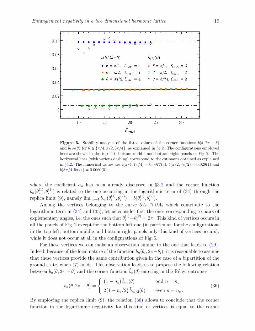
Figure 5. Stability analysis of the fitted values of the corner functions b(θ, 2π − θ)
and b1/2(θ) for θ ∈ {π/4, π/2, 3π/4}, as explained in §4.2. The configurations employed
here are shown in the top left, bottom middle and bottom right panels of Fig. 2. The
horizontal lines (with various dashing) correspond to the estimates obtained as explained
in §4.2. The numerical values are b(π/4, 7π/4) = 0.0977(3), b(π/2, 3π/2) = 0.029(1) and
b(3π/4, 5π/4) = 0.0060(5).
where the coefficient an has been already discussed in §3.2 and the corner function
bn(θ(1)i , θ
(2)i ) is related to the one occurring in the logarithmic term of (34) through the
replica limit (9), namely limne→1 bne(θ(1)i , θ
(2)i ) = b(θ
(1)i , θ
(2)i ).
Among the vertices belonging to the curve ∂A1 ∩ ∂A2 which contribute to the
logarithmic term in (34) and (35), let us consider first the ones corresponding to pairs of
explementary angles, i.e. the ones such that θ(1)i +θ
(2)i = 2π. This kind of vertices occurs in
all the panels of Fig. 2 except for the bottom left one (in particular, for the configurations
in the top left, bottom middle and bottom right panels only this kind of vertices occurs),
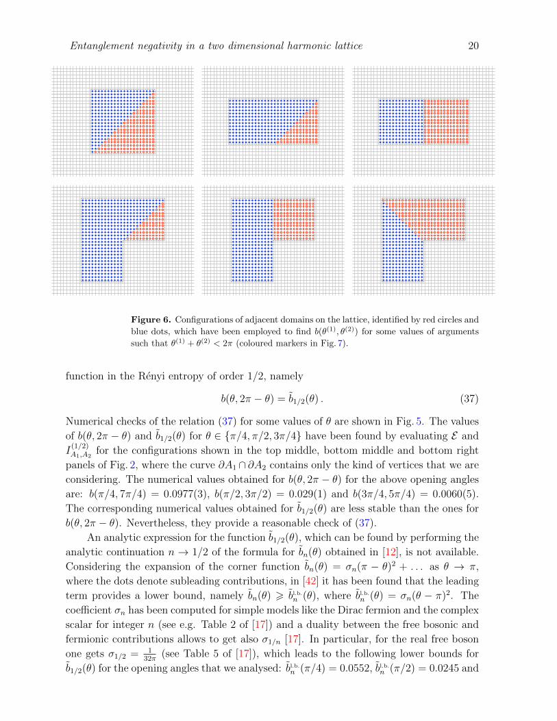
while it does not occur at all in the configurations of Fig. 6.
For these vertices we can make an observation similar to the one that leads to (29).
Indeed, because of the local nature of the function bn(θi, 2π−θi), it is reasonable to assume
that these vertices provide the same contribution given in the case of a bipartition of the
ground state, when (7) holds. This observation leads us to propose the following relation
between bn(θ, 2π − θ) and the corner function bn(θ) entering in the Renyi entropies
bn(θ, 2π − θ) =
{ (1− no
)bno(θ) odd n = no ,
2(1− ne/2
)bne/2(θ) even n = ne .
(36)
By employing the replica limit (9), the relation (36) allows to conclude that the corner
function in the logarithmic negativity for this kind of vertices is equal to the corner
Entanglement negativity in a two dimensional harmonic lattice 20
Figure 6. Configurations of adjacent domains on the lattice, identified by red circles and
blue dots, which have been employed to find b(θ(1), θ(2)) for some values of arguments
such that θ(1) + θ(2) < 2π (coloured markers in Fig. 7).
function in the Renyi entropy of order 1/2, namely
b(θ, 2π − θ) = b1/2(θ) . (37)
Numerical checks of the relation (37) for some values of θ are shown in Fig. 5. The values
of b(θ, 2π − θ) and b1/2(θ) for θ ∈ {π/4, π/2, 3π/4} have been found by evaluating E and
I(1/2)A1,A2
for the configurations shown in the top middle, bottom middle and bottom right
panels of Fig. 2, where the curve ∂A1 ∩ ∂A2 contains only the kind of vertices that we are
considering. The numerical values obtained for b(θ, 2π − θ) for the above opening angles
are: b(π/4, 7π/4) = 0.0977(3), b(π/2, 3π/2) = 0.029(1) and b(3π/4, 5π/4) = 0.0060(5).
The corresponding numerical values obtained for b1/2(θ) are less stable than the ones for
b(θ, 2π − θ). Nevertheless, they provide a reasonable check of (37).
An analytic expression for the function b1/2(θ), which can be found by performing the
analytic continuation n → 1/2 of the formula for bn(θ) obtained in [12], is not available.
Considering the expansion of the corner function bn(θ) = σn(π − θ)2 + . . . as θ → π,
where the dots denote subleading contributions, in [42] it has been found that the leading
term provides a lower bound, namely bn(θ) > bl.b.n (θ), where bl.b.n (θ) = σn(θ − π)2. The
coefficient σn has been computed for simple models like the Dirac fermion and the complex
scalar for integer n (see e.g. Table 2 of [17]) and a duality between the free bosonic and
fermionic contributions allows to get also σ1/n [17]. In particular, for the real free boson
one gets σ1/2 = 132π
(see Table 5 of [17]), which leads to the following lower bounds for
b1/2(θ) for the opening angles that we analysed: bl.b.n (π/4) = 0.0552, bl.b.n (π/2) = 0.0245 and
Entanglement negativity in a two dimensional harmonic lattice 21
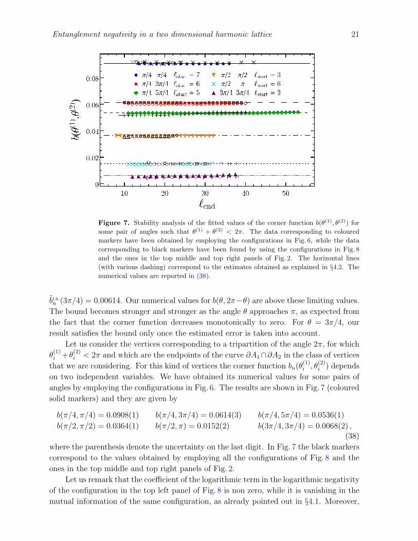
Figure 7. Stability analysis of the fitted values of the corner function b(θ(1), θ(2)) for
some pair of angles such that θ(1) + θ(2) < 2π. The data corresponding to coloured
markers have been obtained by employing the configurations in Fig. 6, while the data
corresponding to black markers have been found by using the configurations in Fig. 8
and the ones in the top middle and top right panels of Fig. 2. The horizontal lines
(with various dashing) correspond to the estimates obtained as explained in §4.2. The
numerical values are reported in (38).
bl.b.n (3π/4) = 0.00614. Our numerical values for b(θ, 2π−θ) are above these limiting values.
The bound becomes stronger and stronger as the angle θ approaches π, as expected from
the fact that the corner function decreases monotonically to zero. For θ = 3π/4, our
result satisfies the bound only once the estimated error is taken into account.
Let us consider the vertices corresponding to a tripartition of the angle 2π, for which
θ(1)i +θ
(2)i < 2π and which are the endpoints of the curve ∂A1∩∂A2 in the class of vertices
that we are considering. For this kind of vertices the corner function bn(θ(1)i , θ
(2)i ) depends
on two independent variables. We have obtained its numerical values for some pairs of
angles by employing the configurations in Fig. 6. The results are shown in Fig. 7 (coloured
solid markers) and they are given by
b(π/4, π/4) = 0.0908(1) b(π/4, 3π/4) = 0.0614(3) b(π/4, 5π/4) = 0.0536(1)
b(π/2, π/2) = 0.0364(1) b(π/2, π) = 0.0152(2) b(3π/4, 3π/4) = 0.0068(2) ,(38)
where the parenthesis denote the uncertainty on the last digit. In Fig. 7 the black markers
correspond to the values obtained by employing all the configurations of Fig. 8 and the
ones in the top middle and top right panels of Fig. 2.
Let us remark that the coefficient of the logarithmic term in the logarithmic negativity
of the configuration in the top left panel of Fig. 8 is non zero, while it is vanishing in the
mutual information of the same configuration, as already pointed out in §4.1. Moreover,
Entanglement negativity in a two dimensional harmonic lattice 22
Figure 8. Configurations of adjacent domains on the lattice, identified by red circles
and blue dots, which have been employed as crosschecks for the values of b(θ(1), θ(2))
given in Fig. 5 and Fig. 7.
such coefficient for the configuration shown in the the bottom left panel of Fig. 2 turns out
to be zero within our numerical errors, both for the negativity and the mutual information,
as expected from the fact that corners do not occur in the continuum limit.
In principle, our numerical analysis allows to find also bn(θ(1)i , θ
(2)i ). Nevertheless,
in order to check the relation (36) we need to know the unusual corrections [43] to the
scaling in 2 + 1 dimensions in order to perform a precise fitting analysis (see e.g. [44]).
4.3. Comments on the continuum limit
The continuum limit of the lattice model (10) considered throughout this manuscript is
described by the massless scalar field in 2 + 1 dimensions, which is a CFT. Denoting by ε
the UV cutoff that must be introduced to regularise the model, the logarithmic negativity
of adjacent domains diverges when ε→ 0.
The numerical results on the lattice discussed above tell us that the expansion of the
logarithmic negativity as ε→ 0 reads
E = αPshared
ε−( ∑
vertices of∂A1 ∩ ∂A2
b(θ(1)i , θ
(2)i )
)log(Pshared/ε) + . . . , (39)
where the coefficient α in front of the area law term is non universal. A similar expression
Entanglement negativity in a two dimensional harmonic lattice 23
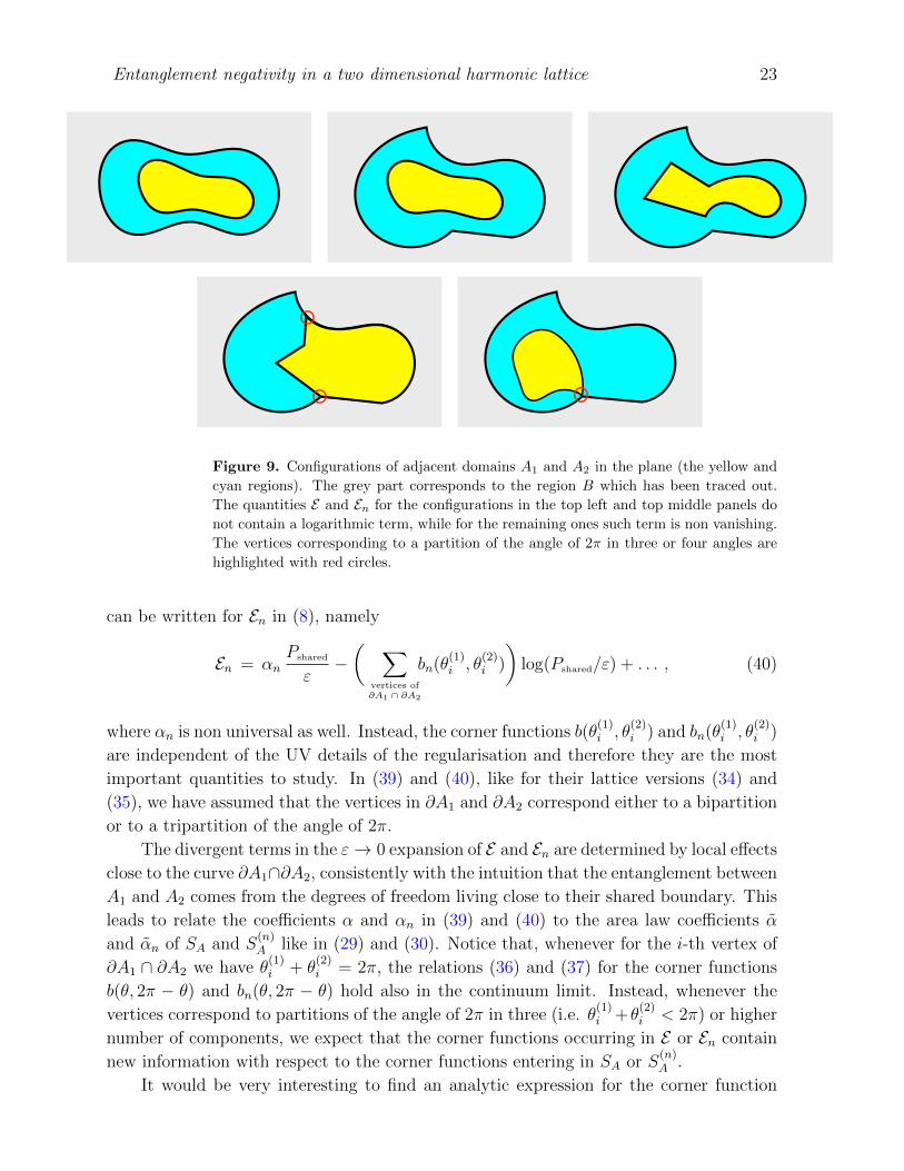
Figure 9. Configurations of adjacent domains A1 and A2 in the plane (the yellow and
cyan regions). The grey part corresponds to the region B which has been traced out.
The quantities E and En for the configurations in the top left and top middle panels do
not contain a logarithmic term, while for the remaining ones such term is non vanishing.
The vertices corresponding to a partition of the angle of 2π in three or four angles are
highlighted with red circles.
can be written for En in (8), namely
En = αnPshared
ε−( ∑
vertices of∂A1 ∩ ∂A2
bn(θ(1)i , θ
(2)i )
)log(Pshared/ε) + . . . , (40)
where αn is non universal as well. Instead, the corner functions b(θ(1)i , θ
(2)i ) and bn(θ
(1)i , θ
(2)i )
are independent of the UV details of the regularisation and therefore they are the most
important quantities to study. In (39) and (40), like for their lattice versions (34) and
(35), we have assumed that the vertices in ∂A1 and ∂A2 correspond either to a bipartition
or to a tripartition of the angle of 2π.
The divergent terms in the ε→ 0 expansion of E and En are determined by local effects
close to the curve ∂A1∩∂A2, consistently with the intuition that the entanglement between
A1 and A2 comes from the degrees of freedom living close to their shared boundary. This
leads to relate the coefficients α and αn in (39) and (40) to the area law coefficients α
and αn of SA and S(n)A like in (29) and (30). Notice that, whenever for the i-th vertex of
∂A1 ∩ ∂A2 we have θ(1)i + θ
(2)i = 2π, the relations (36) and (37) for the corner functions
b(θ, 2π − θ) and bn(θ, 2π − θ) hold also in the continuum limit. Instead, whenever the
vertices correspond to partitions of the angle of 2π in three (i.e. θ(1)i +θ
(2)i < 2π) or higher
number of components, we expect that the corner functions occurring in E or En contain
new information with respect to the corner functions entering in SA or S(n)A .
It would be very interesting to find an analytic expression for the corner function
Entanglement negativity in a two dimensional harmonic lattice 24
b(θ, γ) for any pair of angles θ and γ, where we can assume θ 6 γ. By considering only
the few pairs of angles that we have studied on the lattice, we can make some observations
about the behaviour of this corner function. For instance, when the two angles are equal,
the function b(θ, θ) is decreasing with θ ∈ (0, π] and b(π, π) = 0. Moreover, for fixed
θ 6 π, the function b(θ, γ) is decreasing with γ ∈ (θ, 2π − θ). By comparing Fig. 7 with
Fig. 5, one notices that this is not true anymore when γ is exactly 2π− θ. Such behaviour
is not surprising because in this limit the boundaries of A1 and A2 merge, Pshared changes
abruptly and therefore a continuous behaviour of the divergent terms in the logarithmic
negativity is not expected.
In Fig. 9 we show some illustrative examples of configurations of adjacent regions
in the plane. The grey region is associated to the part B, which has been traced out.
Considering E and En between the yellow domain and the cyan domain, the expressions
(39) and (40) can be employed for all the configurations in Fig. 9 except for the one in
the bottom right panel, where the vertex highlighted by the red circle corresponds to a
partition of the angle of 2π in four parts.
In the configurations shown in the top left and middle panels of Fig. 9 the curve
∂A1 ∩ ∂A2 is smooth; therefore the logarithmic divergence does not occur in E and En.
Instead, in the remaining configurations the curve ∂A1 ∩ ∂A2 contains vertices and the
subleading logarithmic divergence occurs. As for the configuration in the top right panel,
the coefficient of the logarithmic term of E and En is related to the corner functions b(θ)
and bn(θ) entering in the logarithmic term of SA or S(n)A respectively through (36) and
(37). Thus, for the configurations in the top panels of Fig. 9 and assuming that only one
scale ` occurs to determine the logarithmic term, one can construct the following UV
finite quantity
E − 1
2I(1/2)A1,A2
. (41)
For the same configurations, also the following combinations, depending on the parity of
the integer n, are UV finite
Eno −1− no
2I(no)A1,A2
, Ene −(
1− ne2
)I(ne/2)A1,A2
. (42)
The second expression in (42) provides (41) after the analytic continuation ne → 1. In
a 2 + 1 dimensional CFT, the quantities in (41) and (42) should give non trivial scale
invariant functions of the parameters characterising the adjacent domains. For example,
when the adjacent domains are given by a disk of radius Rin and an annulus surrounding
it whose radii are Rin < Rout, the expression (41) should be a model dependent function
of the ratio Rin/Rout. It would be very interesting to develop a method which allows to
get an analytic expression for this function.
The configurations of adjacent domains shown in the bottom panels of Fig. 9 are more
interesting because the corner functions corresponding to the vertices highlighted by the
red circles is not related to the corner functions occurring in the entanglement entropies.
Thus, because of such terms, we expect that the combinations in (41) and (42) diverge
logarithmically for these configurations.
Entanglement negativity in a two dimensional harmonic lattice 25
5. Conclusions
In this manuscript we have investigated the logarithmic negativity E and the moments
of the partial transpose for adjacent domains A1 and A2 in the ground state of a two
dimensional harmonic square lattice with nearest neighbour spring-like interaction. The
regime of massless oscillators in the thermodynamic limit has been considered.
By exploring various configurations of adjacent domains, we have shown that, at
leading order for large domains, the logarithmic negativity and the quantity En introduced
in (8) satisfy an area law in terms of the length of the shared curve ∂A1∩∂A2, suggesting a
relation between the coefficient of the area law term in these quantities and the coefficient
of the area law term in the Renyi entropies.
A subleading universal logarithmic term occurs in E and En whenever the shared
curve contains vertices, being its endpoints included among them. The values of the
corner function of E have been obtained for some pairs of angles. For the vertices of
∂A1 ∩ ∂A2 corresponding to pairs of explementary angles, we have proposed that the
corner function of En is related to the corner function entering in the Renyi entropies [12].
This relation implies that the corner function of E for this kind of vertices coincides with
the corner function of the Renyi entropy of order 1/2. This statement has been supported
by numerical evidences shown in Fig. 5.
As for the vertices of the curve ∂A1 ∩ ∂A2 corresponding to a tripartition of the
angle of 2π, their contribution to the logarithmic term in E and En is characterised by a
new corner function which depends on two independent angular variables. The numerical
values of this corner function for E have been given in (38) for some pair of angles (see
also Fig. 7).
Let us conclude with some open questions. It would be interesting to provide further
checks of (37). In particular, the analytic continuation to n = 1/2 of the corner function
found by Casini and Huerta [12] should be performed. More importantly, a method should
be found to compute analytically the corner functions b(θ, γ) and bn(θ, γ) for the vertices
partitioning the angle of 2π in three parts. By analogy with the results of [16] obtained for
the corner function of SA, it could be interesting to study the corner function b(θ, θ) for
equal angles as θ → π−. In order to extract reliable numerical results for the logarithmic
term of En from the fit of the lattice data, the unusual corrections to the scaling must be
studied, extending the analysis done by Cardy and Calabrese [43] in 1 + 1 dimensions.
Finally, it is worth studying the corner contributions to E and En for other models, both
on the lattice and in the continuum.
Acknowledgements
We are grateful in particular to Pasquale Calabrese, John Cardy, Horacio Casini and
Marina Huerta for useful discussions and correspondence. We thank Vincenzo Alba,
Mario Collura, Viktor Eisler, Veronika Hubeny, Mukund Rangamani, German Sierra,
William Witczak-Krempa and Zoltan Zimboras for useful conversations. ET would like
Entanglement negativity in a two dimensional harmonic lattice 26
to thank the Instituto de Fisica Teorica (IFT UAM-CSIC) in Madrid for hospitality during
part of this work and its support via the Centro de Excelencia Severo Ochoa Program
under Grant SEV-2012-0249. ET is grateful to Princeton University, MIT, Brandeis
University and UC Davis for the warm hospitality during the final part of this work.
AC acknowledges support from MINECO (grant MTM2014-54240-P) and Comunidad de
Madrid (grant QUITEMAD+-CM, ref. S2013/ICE-2801). AC has received funding from
the European Research Council (ERC) under the European Union’s Horizon 2020 research
and innovation programme (grant agreement No 648913). ET has been supported by the
ERC under Starting Grant 279391 EDEQS.
References
[1] L. Amico, R. Fazio, A. Osterloh and V. Vedral, Rev. Mod. Phys. 80, 517 (2008);
J. Eisert, M. Cramer and M. B. Plenio, Rev. Mod. Phys. 82, 277 (2010);
P. Calabrese, J. Cardy and B. Doyon (Eds), J. Phys. A 42, 500301 (2009), special issue.
[2] B. Groisman, S. Popescu and A. Winter, Phys. Rev. A 72, 032317 (2005);
M. Nielsen and I. Chuang, Quantum Computation and Quantum Information, Cambridge
University Press, Cambridge UK, 2000.
[3] M. Wolf, F. Verstraete, M. Hastings and I. Cirac, Phys. Rev. Lett. 100, 070502 (2008).
[4] R. Sorkin, Tenth International Conference on General Relativity and Gravitation, Padova 4-9 July
1983, Contributed Papers, vol. II, 734, arXiv:1402.3589;
L. Bombelli, R. Koul, J. Lee and R. Sorkin, Phys. Rev. D 34 (1986) 373;
M. Srednicki, Phys. Rev. Lett. 71 (1993) 666.
[5] M. B. Plenio, J. Eisert, J. Dressig and M. Cramer, Phys. Rev. Lett. 94, 060503 (2005);
M. Cramer, J. Eisert, M. B. Plenio and J. Dreissig, Phys. Rev. A 73, 012309 (2006);
T. Barthel, M.-C. Chung and U. Schollwoeck, Phys. Rev. A 74, 022329 (2006);
M. Huerta, Phys. Lett. B 710 691 (2012).
[6] G. Vidal, J. Latorre, E. Rico and A. Kitaev, Phys. Rev. Lett. 90, 227902 (2003);
J. Latorre, E. Rico, and G. Vidal, Quant. Inf. Comp. 4, 048 (2004).
[7] M. Wolf, Phys. Rev. Lett. 96, 010404 (2006);
D. Gioev and I. Klich, Phys. Rev. Lett. 96, 100503 (2006).
[8] C. Holzhey, F. Larsen, and F. Wilczek, Nucl. Phys. B 424, 443 (1994);
C. Callan and F. Wilczek, Phys. Lett. B 333, 55 (1994);
P. Calabrese and J. Cardy, J. Stat. Mech. P06002 (2004);
P. Calabrese and J. Cardy, J. Phys. A 42, 504005 (2009).
[9] M. Caraglio and F. Gliozzi, JHEP 0811:076 (2008);
S. Furukawa, V. Pasquier, and J. Shiraishi, Phys. Rev. Lett. 102, 170602 (2009);
P. Calabrese, J. Cardy, and E. Tonni, J. Stat. Mech. P11001 (2009);
M. Headrick, Phys. Rev. D 82, 126010 (2010);
P. Calabrese, J. Cardy and E. Tonni, J. Stat. Mech. P01021 (2011);
A. Coser, L. Tagliacozzo and E. Tonni, J. Stat. Mech. P01008 (2014).
[10] C. Agon, M. Headrick, D. Jafferis and S. Kasko, Phys. Rev. D 89, 025018 (2014).
[11] C. De Nobili, A. Coser and E. Tonni, J. Stat. Mech. P06021 (2015).
[12] H. Casini and M. Huerta, Nucl. Phys. B 764, 183 (2007).
[13] H. Casini, M. Huerta and L. Leitao, Nucl. Phys. B 814, 594 (2009).
[14] H. Casini and M. Huerta, J. Phys. A 42, 504007 (2009).
[15] A. Kallin, K. Hyatt, R. Singh and R. Melko, Phys. Rev. Lett. 110, 135702 (2013);
E. Stoudenmire, P. Gustainis, R. Johal, S. Wessel and R. Melko, Phys. Rev. B 90, 235106 (2014);
A. Kallin, E. Stoudenmire, P. Fendley, R. Singh and R. Melko, J. Stat. Mech. P06009 (2014);
Entanglement negativity in a two dimensional harmonic lattice 27
J.-M. Stephan, S. Furukawa, G. Misguich and V. Pasquier, Phys. Rev. B 80, 184421 (2009);
R. Singh, R. Melko and J. Oitmaa, Phys. Rev. B 86, 075106 (2012);
S. Humeniuk and T. Roscilde, Phys. Rev. B 86, 235116 (2012);
T. Devakul and R. Singh, Phys. Rev. B 90, 064424 (2014);
N. Laflorencie, D. Luitz and F. Alet, Phys. Rev. B 92, 115126 (2015).
[16] P. Bueno, R. Myers and W. Witczak-Krempa, Phys. Rev. Lett. 115, 021602 (2015);
P. Bueno and R. Myers, JHEP 1508 (2015) 068.
[17] P. Bueno, R. Myers and W. Witczak-Krempa, JHEP 1509 (2015) 091.
[18] S. Ryu and T. Takayanagi, Phys. Rev. Lett. 96, 181602 (2006); JHEP 0608:045 (2006).
[19] N. Drukker, D. Gross and H. Ooguri, Phys. Rev. D 60, 125006 (1999);
T. Hirata and T. Takayanagi, JHEP 0702:042 (2007);
P. Fonda, L. Giomi, A. Salvio and E. Tonni, JHEP 1502 (2015) 005;
P. Fonda, D. Seminara and E. Tonni, JHEP 1512 (2015) 037.
[20] J. Cardy, J. Phys. A 46 285402 (2013).
[21] A. Peres, Phys. Rev. Lett. 77, 1413 (1996);
K. Zyczkowski, P. Horodecki, A. Sanpera and M. Lewenstein, Phys. Rev. A 58, 883 (1998);
J. Eisert and M. Plenio, J. Mod. Opt. 46, 145 (1999);
J. Lee, M. Kim, Y. Park and S. Lee, J. Mod. Opt. 47, 2151 (2000);
G. Vidal and R. F. Werner, Phys. Rev. A 65, 032314 (2002);
M. Plenio, Phys. Rev. Lett. 95, 090503 (2005);
J. Eisert, quant-ph/0610253.
[22] P. Calabrese, J. Cardy and E. Tonni, Phys. Rev. Lett. 109, 130502 (2012).
[23] P. Calabrese, J. Cardy and E. Tonni, J. Stat. Mech. P02008 (2013).
[24] P. Calabrese, L. Tagliacozzo and E. Tonni, J. Stat. Mech. P05002 (2013);
V. Alba, J. Stat. Mech. P05013 (2013);
A. Coser, E. Tonni and P. Calabrese, J. Stat. Mech. P033116 (2016);
A. Coser, E. Tonni and P. Calabrese, J. Stat. Mech. 053109 (2016);
C. Herzog and Y. Wang, J. Stat. Mech. 073102 (2016).
[25] P. Calabrese, J. Cardy and E. Tonni, J. Phys. A 48, 015006 (2015).
[26] V. Eisler and Z. Zimboras, New J. Phys. 17, 053048 (2015).
[27] A. Coser, E. Tonni and P. Calabrese, J. Stat. Mech. P08005 (2015).
[28] P.-Y. Chang and X. Wen, Phys. Rev. B 93, 195140 (2016).
[29] O. Blondeau-Fournier, O. Castro-Alvaredo and B. Doyon, J. Phys. A 48, 125401 (2016).
[30] A. Coser, E. Tonni and P. Calabrese, J. Stat. Mech. P12017 (2014).
[31] V. Eisler and Z. Zimboras, New J. Phys. 16, 123020 (2014);
M. Hoogeveen and B. Doyon, Nucl. Phys. B 898, 78 (2015);
X. Wen, P.-Y. Chang and S. Ryu, Phys. Rev. B 92, 075109 (2015).
[32] H. Wichterich, J. Molina-Vilaplana and S. Bose, Phys. Rev. A 80, 010304 (2009);
J. Anders and A. Winter, Quantum Inf. Comput. 8, 0245 (2008);
J. Anders, Phys. Rev. A 77, 062102 (2008);
A. Ferraro, D. Cavalcanti, A. Garcia-Saez and A. Acin, Phys. Rev. Lett. 100, 080502 (2008);
D. Cavalcanti, A. Ferraro, A. Garcia-Saez and A. Acin, Phys. Rev. A 78, 012335 (2008);
H. Wichterich, J. Vidal and S. Bose, Phys. Rev. A 81, 032311 (2010);
A. Bayat, P. Sodano and S. Bose, Phys. Rev. Lett. 105, 187204 (2010); Phys. Rev. B 81, 064429
(2010);
P. Sodano, A. Bayat and S. Bose, Phys. Rev. B 81, 100412 (2010);
A. Bayat, S. Bose, P. Sodano and H. Johannesson, Phys. Rev. Lett. 109, 066403 (2012);
B. Alkurtass, A. Bayat, I. Affleck, S. Bose, H. Johannesson, P. Sodano, E. Sørensen and K. Le
Hur, Phys. Rev. B 93, 081106 (2016);
C. Chung, V. Alba, L. Bonnes, P. Chen and A. Lauchli, Phys. Rev. B 90, 064401 (2014).
[33] C. Castelnovo, Phys. Rev. A 88, 042319 (2013); Phys. Rev. A 89, 042333 (2014);
Entanglement negativity in a two dimensional harmonic lattice 28
Y. A. Lee and G. Vidal, Phys. Rev. A 88, 042318 (2013);
R. Santos, V. Korepin and S. Bose, Phys. Rev. A 84, 062307 (2011);
R. Santos and V. Korepin, J. Phys. A 45, 125307 (2012);
X. Wen, S. Matsuura and S. Ryu, Phys. Rev. B 93, 245140 (2016).
[34] V. Eisler and Z. Zimboras, Phys. Rev. B 93, 115148 (2016).
[35] N. Sherman, T. Devakul, M. Hastings and R. Singh, Phys. Rev. E 93, 022128 (2016),
[36] M. Rangamani and M. Rota, JHEP 1410 (2014) 60;
M. Kulaxizi, A. Parnachev and G. Policastro, JHEP 1409 (2014) 010.
[37] I. Peschel and M.-C. Chung, J. Phys. A 32, 8419 (1999);
I. Peschel, J. Phys. A 36, L205 (2003);
A. Botero and B. Reznik, Phys. Rev. A 70, 052329 (2004);
I. Peschel and V. Eisler, J. Phys. A 42, 504003 (2009).
[38] R. Simon, Phys. Rev. Lett. 84, 2726 (2000);
K. Audenaert, J. Eisert, M. Plenio and R. Werner, Phys. Rev. A 66, 042327 (2002).
[39] H. Casini, M. Huerta, R. Myers and A. Yale, JHEP 1510 (2015) 003.
[40] J. Cardy, talk given at KITP for the conference Closing the entanglement gap: Quantum information,
quantum matter and quantum fields, June 1-5, 2015;
B. Swingle, arXiv:1304.6402.
[41] F. Gliozzi and L. Tagliacozzo, J. Stat. Mech. P01002 (2010).
[42] P. Bueno and W. Witczak-Krempa Phys. Rev. B 93, 045131 (2016).
[43] J. Cardy and P. Calabrese, J. Stat. Mech. P04023 (2010).
[44] S. Sahoo, E. Stoudenmire, J.-M. Stephan, T. Devakul, R. Singh and R. Melko, Phys. Rev. B 93,
085120 (2016).
Top Related