


Languages
Pages
Legal


Co
pyri
gh
t R
. J
an
ow
–S
pri
ng
2012
Physics 111 Lecture 02
Motion in One Dimension
SJ 8th Ed.: Ch. 2.1 –2.8
•Introduction to motion & kinematics,
definitions
•Position and Displacement
•Average velocity, average speed
•Instantaneous velocity and speed
•Acceleration
•Motion diagrams
•Constant acceleration -a special case
•Kinematic equations
•Free fall
•Another look at constant acceleration
(kinematic equations derived using
calculus).
2.1
Po
sit
ion
, V
elo
cit
y,
an
d S
pe
ed
2.2
Ins
tan
tan
eo
us
Ve
loc
ity a
nd
Sp
ee
d
2.3
A p
art
icle
un
de
r C
on
sta
nt
Ve
loc
ity
2.4
Ac
ce
lera
tio
n
2.5
Mo
tio
n D
iag
ram
s
2.6
A p
art
icle
un
de
r C
on
sta
nt
Ac
ce
lera
tio
n
2.7
Fre
e F
all
2.8
Kin
em
ati
c E
qu
ati
on
s D
eri
ve
d
fro
m C
alc
ulu
s

Co
pyri
gh
t R
. J
an
ow
–S
pri
ng
2012
Motion -Kinematics
Mech
anics describes motion resulting from
interactions betw
een
masses (m
atter) and
forces.
•“Kinematics”: very little physics
describes motion but ignores the causes
•“D
ynamics”
invoke
s “forces”
that cause m
otion
Kinematic motion concepts:
•Position x(t) & displacement ∆ ∆∆∆x
•Rates of change
•Velocity v(t) & spe
ed
•Acceleration a(t)
Abstractions –
mod
eling assum
ptions:
•Point ob
jects called “pa
rticles”
–infinitesimally
small, no shape
, no spin, no distortion, …
•1 dimensional world
•Motion variables position, displacement, velocity &
acceleration only along + &
-x-axis

Co
pyri
gh
t R
. J
an
ow
–S
pri
ng
2012
Position
Position: an ob
ject’s location
measured relative to a chosen
reference point
(the origin of a
coordinate system).
The road sign in the diagram is
used as the origin.
The position is the displacement
from
the origin.
The position-
time graph
show
s the
location of the particle (car) at every
time in some range.
Points betw
een measurements are
interpolated guesses.
The function x(t) ge
nerating the curve
is continuous and
smooth
(differentiable).

Co
pyri
gh
t R
. J
an
ow
–S
pri
ng
2012
Displacement & Position
)t(
x)
t(x
x
x
xi
fi
f
rr
rr
r− −−−
= ===− −−−
≡ ≡≡≡∆ ∆∆∆
Language
:∆ ∆∆∆
“delta”means difference
Often it shrinks to infinitesimal size
i.e:
∆ ∆∆∆x
� ���dx
� ���0
)t(
x
x
)t(
x
xi
if
f
rr
rr
≡ ≡≡≡≡ ≡≡≡
Positions
ti
me
o
f
fun
cti
on
as
o
sit
ion
p
)t(x
≡ ≡≡≡
rUsually w
e w
ant to find
this.
orig
inx
ix
f∆ ∆∆∆
x
x(t
i)x(t
f)
[x(t
)] an
d [∆ ∆∆∆
x]
= le
ng
th, S
I u
nit
s a
re m
ete
rs
Displacement is a particle’s cha
nge in position(a vector)
during some time interval
A scalar
t
t
ti
f∆ ∆∆∆
≡ ≡≡≡− −−−

Co
pyri
gh
t R
. J
an
ow
–S
pri
ng
2012
The Difference between Distance Covered and Displacement
A basketball player starts in
the center, runs back and
forth
to the baskets a couple of times
(See graph
of x(t)).
L = length of the court
∆ ∆∆∆x= displacement
d = distance covered
(always positive)
2/L
xx
xa
ba,
b= ===
− −−−≡ ≡≡≡
∆ ∆∆∆2/
Ld
a,b
= ===
2/L
xx
xa
ca,
c− −−−
= ===− −−−
≡ ≡≡≡∆ ∆∆∆
Ld
a,c
23= ===
2/L
xx
xa
ea,
e− −−−
= ===− −−−
≡ ≡≡≡∆ ∆∆∆
Ld
a,e
27= ===
2/L
xx
xa
da,
d= ===
− −−−≡ ≡≡≡
∆ ∆∆∆L
da,
d25
= ===
0= ===
− −−−≡ ≡≡≡
∆ ∆∆∆a
fa,f
xx
xL
da,f
4= ===
t �
a
b
c
d
e
fx(t
)

Co
pyri
gh
t R
. J
an
ow
–S
pri
ng
2012
Average Velocity (a Vector)
Th
e a
vera
ge v
elo
cit
yo
f a p
art
icle
du
rin
g s
om
e t
ime in
terv
al is
th
e
dis
pla
cem
en
td
ivid
ed
by t
he t
ime in
terv
al fo
r th
e d
isp
lacem
en
t to
occu
r –
the a
vera
ge r
ate
of
ch
an
ge o
f p
osit
ion
du
rin
g t
he in
terv
al
if
if
avg
tt
xx
tx
v
− −−−− −−−= ===
∆ ∆∆∆∆ ∆∆∆≡ ≡≡≡
rr
rr
Th
e x
in
dic
ate
s m
oti
on
alo
ng
th
e x
-axis
Dimensions of velocity &
/or speed are length / time [L/T
]SI units are m
/s
ft
to it
fr
om
seg
men
t
lin
e
of
lo
pe
savg
v≡ ≡≡≡
Example:
m
/s.
.
.
..
v
m .
s.
x
.
t
m.
s
.
x
.t
avg
bb
aa
46
16
44
9
00
60
01
3
00
13
49
00
66
4
= ===− −−−− −−−
= ===
= ==== ===
= ==== ===
What would v
avgbe betw
een
a,c
or b,c?
On position vstime graph
:t �
a
b
∆x
ba
∆t b
a
c
x(t
)

Co
pyri
gh
t R
. J
an
ow
–S
pri
ng
2012
Average Speed (a Scalar, Positive Quantity)
Th
e a
vera
ge s
peed
of
a p
art
icle
du
rin
g s
om
e t
ime in
terv
al is
th
e
tota
l d
ista
nce t
ravele
d d
ivid
ed
by t
he len
gth
of
the t
ime in
terv
al.
if
ere
dco
vce
tan
dis
to
tal
avg
tt
td
s
− −−−= ===
∆ ∆∆∆∆ ∆∆∆≡ ≡≡≡
Dim
ensions: L/T.
SI units: m/s
•Drive 50 km east at 50 km/h
r for 1 hour
•Stop for 1 hour
•Drive 50 km w
est for 2 hours at 25 km/h
r
km
x
50
+ +++= ===
∆ ∆∆∆
Average
Velocity:
0
)x
(x
)x
x(
x1
tot
= ===− −−−
= ===− −−−
+ +++− −−−
= ===∆ ∆∆∆
50
50
21
2h
ou
rs
t t
ot
4= ===
∆ ∆∆∆
0
tx
v
to
t
tot
tot
,a
vg
= ===∆ ∆∆∆∆ ∆∆∆
= ===
Example
km
x
50
− −−−= ===
∆ ∆∆∆
km
x
0= ===
∆ ∆∆∆
x1
x2
Average
Spe
ed:
km
km
50
km
dto
t100
50
= ===+ +++
+ +++= ===
∆ ∆∆∆h
ou
rs
t t
ot
4= ===
∆ ∆∆∆ km
/hr
25
ho
urs
4
km
100
td
s
to
t
tot
tot
,a
vg
= ==== ===
∆ ∆∆∆∆ ∆∆∆= ===

Co
pyri
gh
t R
. J
an
ow
–S
pri
ng
2012
Instantaneous Velocity and Speed
“In
sta
nta
neo
us”
mean
s “
at
so
me g
iven
tim
e in
sta
nt”
vin
stis
va
vg
over
an
in
fin
itesim
alin
terv
al
∆ ∆∆∆t� ���
0
Limiting process:
•T
he c
ho
rd’s
slo
pe i
s t
he a
vera
ge v
elo
cit
y.
•L
et
∆ ∆∆∆t� ���
0,
en
clo
sin
g t
fo
r th
e r
ed
do
t.
•T
he c
ho
rds b
eco
me s
ucc
essiv
ely
b
ett
er
ap
pro
xim
ati
on
s t
o t
he t
an
gen
tat
the t
ime o
f in
tere
st.
.
Th
e i
nsta
nta
neo
us v
elo
cit
y i
s t
he r
ate
of
ch
an
ge o
f p
osit
ion
at
the
tim
e o
f in
tere
st;
i.e
. th
e s
lop
e o
f th
e t
an
gen
t li
ne o
n a
n x
(t)
gra
ph
d
t
dx
tx
Lim
v L
imv
v
tavg
tin
st
≡ ≡≡≡∆ ∆∆∆∆ ∆∆∆
= ===≡ ≡≡≡
≡ ≡≡≡→ →→→
∆ ∆∆∆→ →→→
∆ ∆∆∆0
0
The limit define
s the time derivative
of the position function
The instantaneous speedis the m
agnitud
e
of the instantane
ous velocity
|v
|
s
ins
t≡ ≡≡≡
t �
tangent
line
∆ ∆∆∆x
0chord
∆ ∆∆∆t 0

Co
pyri
gh
t R
. J
an
ow
–S
pri
ng
2012
Finding instantaneous velocity when the position
is known as a function of time
Approximate M
ethod
: Calculate the average
velocity over a
“sufficiently short”
interval (squeeze
its duration)
Calculus M
ethod
: Find the derivative of the position function,
prod
ucing the velocity as a function of time.
Evaluate v
(t)at time t
.1
− −−−= ===
nn
kn
t]
kt
[d
td E
xam
ple
1:
Fin
d v
(t)
wh
ere
:)
t -(t
k
x
(t
)x
0
0+ +++
= ===
So
luti
on
:
dt
dt
k
]
[kt
dtd
[kt]
dtd
dt
dx
dt
dx
(t)
v
00
= ===− −−−
+ +++= ===
= ===
k
(t
)v
= ===∴ ∴∴∴
Constant
Exam
ple
2:
Fin
d v
(t=
3.5
s)
wh
ere
:m
t
2.1
t
9.2
7.8
(t)
x
3− −−−
+ +++= ===
9.2
6.3
t
t
)(3)
(2
.1
9.2
(t
)x
dtd
v(t
)
22
+ +++− −−−
= ===− −−−
= ==== ===
So
luti
on
:
m/s
68
9.2
6.3
(3.5
)
3.5
)
v(t
2= ===
+ +++− −−−
= ==== ===
Co
pyri
gh
t R
. J
an
ow
–S
pri
ng
2012
Motion with constant velocity (Special Case)
Slope
of position vs. time graph
is constant
-x
0is
th
e y
-in
terc
ep
t =
in
itia
l co
ord
ina
te-
Ave
rag
e a
nd
in
sta
nta
neo
us v
elo
cit
ies
are
eq
ual
0 t
x - x(t
)
tx
v
v
0a
vg
− −−−= ===
∆ ∆∆∆∆ ∆∆∆= ===
= ===
t
v
x
x(t
)
0+ +++
= ===
Equation for v(t)is a straight line
Graph
of velocity versus time
-v(t
)=
co
nsta
nt
v0
for
an
y t
ime
-D
isp
lacem
en
t =
x –
x0
t
v
co
vere
d
ista
nce
d
0= ===
Th
e d
isp
lacem
en
t is
th
e a
rea b
etw
een
th
e t
ime a
xis
an
d t
he c
urv
e o
n a
velo
cit
y v
ers
us t
ime g
rap
h.
t
v0
∆ ∆∆∆t
v(t
)
velo
cit
y =
co
nsta
nt
t
∆ ∆∆∆t
x(t
)
slo
pe =
velo
cit
y (
co
nsta
nt)
x0
∆ ∆∆∆x

Co
pyri
gh
t R
. J
an
ow
–S
pri
ng
2012
Average and Instantaneous Acceleration
Ac
cele
rati
on
is t
he r
ate
of
ch
an
ge o
f velo
cit
yIn
sta
nta
neo
us a
ccele
rati
on
a(t
) is
th
e s
lop
e o
f a v
elo
cit
y-t
ime
gra
ph
v(t
)
Limiting process:
Th
e c
ho
rd r
ep
resen
ts a
vera
ge
accele
rati
on
. L
et
∆ ∆∆∆t� ���
0.
tv
a a
vg
∆ ∆∆∆∆ ∆∆∆= ===
Average
Acceleration:
Dim
en
sio
ns
: [
a]
=
L /
T2
Un
its
: m
/s2,
ft/s
2
Vecto
r: i
n 1
D c
an
be j
us
t +
or
-
t � ���
tangent
line
∆ ∆∆∆v
chord
∆ ∆∆∆t
20
0d
txd
dt
dv
tv
Lim
a L
ima
a
2
tavg
tin
st
= ==== ===
∆ ∆∆∆∆ ∆∆∆= ===
≡ ≡≡≡≡ ≡≡≡
→ →→→∆ ∆∆∆
→ →→→∆ ∆∆∆
Instantane
ous acceleration is the time derivative of the velocity function
“deceleration”means slowing dow
n:
v
a
n
eg
ati
ve
is
ro
r
Wh
at
accele
rati
on
do
es e
ach
se
gm
en
t
a,…
e
rep
rese
nt?
v(t
)a
bc
de
!*?
!*? !*
?
!*?

Co
pyri
gh
t R
. J
an
ow
–S
pri
ng
2012
Motion Diagrams
Co
nsta
nt
velo
cit
y.
Ac
cele
rati
on
is z
ero
Nothing quantitative –just an aid to visualize what’s happening
-Snapshots at later and later equally spaced times
Ac
cele
rati
on
co
nsta
nt
an
d
alo
ng
in
itia
l velo
cit
y
Ac
cele
rati
on
co
nsta
nt
an
d
op
po
sit
e t
o
init
ial
velo
cit
y
An o
bje
ct
spe
eds u
p w
he
n v
and
aare
in t
he s
am
e d
irection.
It s
low
s d
ow
n w
hen v
and
aare
in o
pposite d
irectio
ns.

Co
pyri
gh
t R
. J
an
ow
–S
pri
ng
2012
Kinematic Equations –Constant Acceleration
•C
an
be u
sed
fo
r o
ne d
imen
sio
nal
mo
tio
n o
f an
y p
art
icle
u
nd
er
co
nsta
nt
accele
rati
on
.•
Ap
pli
cab
le t
o:
gra
vit
y,
co
nsta
nt
forc
es,
eq
uilib
riu
m
bu
t n
ot
c
ircu
lar
mo
tio
n,
vari
ab
le f
orc
es
•A
sm
all
set
of
tracta
ble
fo
rmu
las f
or
co
nsta
nt
accele
rati
on
The m
ost useful ones [see also table 2.1]:
For the particular case
0
a
= ===
v
v
0f
= ===
t
v
x
x
00
f= ===
− −−−
Co
nsta
nt
velo
cit
y
Dis
tan
ce g
row
s lin
earl
y w
ith
tim
e
t a
v
v
0
f+ +++
= ===
2
210
0f
t a
t
v
x
x
+ +++
= ===− −−−
)x
2a(x
v
v
f
2 02 f
0− −−−
+ +++= ===
t)v
(v
x
x
0f
210
f+ +++
= ===− −−−
Ju
sti
ficati
on
s
foll
ow
2.1
3
2.1
6
2.1
7
2.1
5
t =
tf
t 0 =
0
NO
TE
:

Co
pyri
gh
t R
. J
an
ow
–S
pri
ng
2012
Kinematics Formulas via Velocity-time Graph
Equation 2.13:
t a
v
v
0
f+ +++
= ===
ais constant, so
v(t
)is a straight line
v0
is the slope
-intercept
t
v -
v
a
a
0
fa
vg
≡ ≡≡≡= ===
Or, rearrange the definition:
Constantacceleration
Equation 2.16:
Thedisplacement d
(t)is the area
betw
een
v(t
)and
the time axis on
a velocity vs. time graph
Are
a
Are
a
x
x
d(t
)
0f
ΙΙ ΙΙΙΙ
ΙΙ+ +++
Ι ΙΙΙ= ===
− −−−= ===
v(t
)
v(t
) g
rap
hS
lop
e =
a
v0
vf
at
t
Are
aΙ
Ι
Ι
Ι
= v
0t
Are
aΙΙ
ΙΙ
ΙΙ
ΙΙ
=
½at2
v0
2
210
0f
t a
t
v
x
x
+ +++
= ===− −−−
Or, integrate Eq. 2.13
Equation for a parabola
Equations 2.13 and
2.16 can
gene
rate the others on prece
ding slide:
Or, differentiate Eq. 2.16

Co
pyri
gh
t R
. J
an
ow
–S
pri
ng
2012
Kinematics Formulas Discussion, Continued
Equation 2.15:
The displacement d
(t)is the average
velocity m
ultiplied by the time
Constantacceleration
Equation 2.17:
t ]v
[v
tv
x
x
d(t
)
f21
avg
0f
0+ +++
= ===≡ ≡≡≡
− −−−≡ ≡≡≡
Solve Eq2.13 for the time:
t a
v
v
0
f+ +++
= ===a
v
v
t
0
f− −−−
= ===
2
210
0f
t a
t
v
x
x
+ +++
= ===− −−−
2
0f
210
f0
0f
a
vv
a
a
vv
v
x
x
− −−−
+ +++− −−−
= ===− −−−
Eliminate time t
in Eq2.16 and
simplify:
avv
a
v
av
a
v
avv
x
x
f
00
21f
210
f0
0f
− −−−+ +++
+ +++− −−−
= ===− −−−
22
2
v
v
]x
[x
a 2
f
00
f2
2+ +++
− −−−= ===
− −−−
)x
2a(x
v
v
f
2 02 f
0− −−−
+ +++= ===
∴ ∴∴∴
xf–
x0
= d
isp
lacem
en
t
oft
en
den
ote
d d
(t)
or
∆ ∆∆∆x
Co
pyri
gh
t R
. J
an
ow
–S
pri
ng
2012
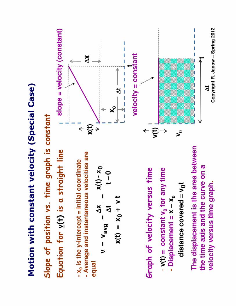
Reading Graphs of Position, Velocity, and Acceleration vs. Time
•Th
e s
lop
e o
f th
e c
urv
e i
s t
he
velo
cit
y•T
he c
urv
ed
lin
e i
nd
ica
tes
th
e v
elo
cit
y i
s c
han
gin
g
•Th
ere
fore
, accele
rati
on
is n
on
-zero
•If
a is
co
ns
tan
t, t
he c
urv
e is
a p
ara
bo
la
•T
he a
rea
un
der
the c
urv
e is
me
an
ing
less
Graph
of
x(t
)versus time
•Th
e s
lop
e g
ives
th
e a
ccele
rati
on
•Th
e s
traig
ht
lin
e in
dic
ate
s a
co
nsta
nt
acce
lera
tio
n•T
his
mig
ht
be t
he d
eri
va
tive o
f th
e c
urv
e a
bo
ve
•T
he a
rea
un
der
the c
urv
e is
th
e d
isp
lace
men
t,w
hic
h c
an
be n
eg
ati
ve
wh
ere
v(t
) is
neg
ati
ve
Graph
of
v(t
)versus time
Graph
of
a(t
)versus time
•Th
e z
ero
slo
pe
in
dic
ate
s a
co
ns
tan
t acce
lera
tio
n
•T
he a
rea
un
der
the c
urv
e is
th
e c
han
ge
in
ve
loc
ity d
uri
ng
th
e t
ime
in
terv
al:
∆ ∆∆∆
v=
at
Co
pyri
gh
t R
. J
an
ow
–S
pri
ng
2012
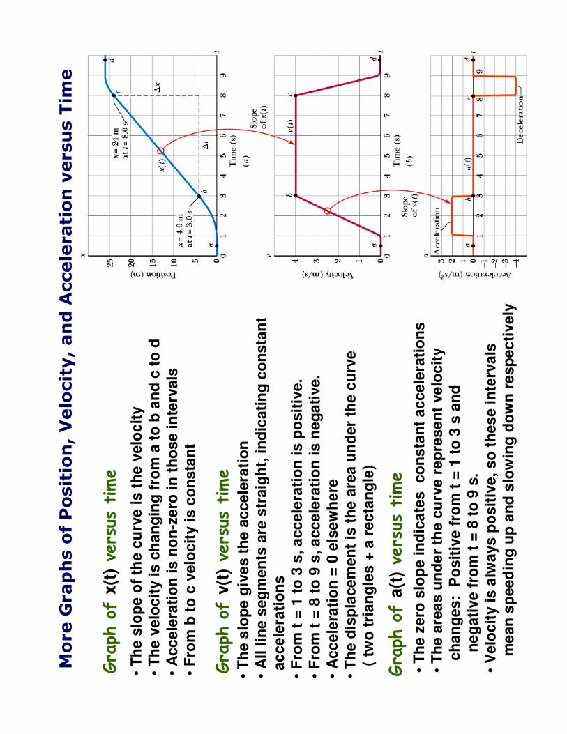
More Graphs of Position, Velocity, and Acceleration versus Time
•T
he s
lop
e o
f th
e c
urv
e i
s t
he
velo
cit
y•
Th
e v
elo
cit
y i
s c
han
gin
g f
rom
a t
o b
an
d c
to
d
•A
cce
lera
tio
n is
no
n-z
ero
in
th
ose in
terv
als
•F
rom
b t
o c
velo
cit
y i
s c
on
sta
nt
Graph
of
x(t
)versus time
•T
he s
lop
e g
ive
s t
he
accele
rati
on
•A
ll l
ine
seg
me
nts
are
str
aig
ht,
in
dic
ati
ng
co
nsta
nt
accele
rati
on
s
•F
rom
t =
1 t
o 3
s, accele
rati
on
is p
osit
ive.
•
Fro
m t
= 8
to
9 s
, accele
rati
on
is n
eg
ati
ve
.•
Acce
lera
tio
n =
0 e
lsew
here
•T
he d
isp
lace
men
t is
th
e a
rea u
nd
er
the
cu
rve
( tw
o t
rian
gle
s +
a r
ecta
ng
le)
Graph
of
v(t
)versus time
Graph
of
a(t
)versus time
•T
he z
ero
slo
pe i
nd
ica
tes
co
nsta
nt
acce
lera
tio
ns
•T
he a
reas
un
de
r th
e c
urv
e r
ep
resen
t ve
loc
ity
ch
an
ges
: P
os
itiv
e f
rom
t =
1 t
o 3
s a
nd
neg
ati
ve
fro
m t
= 8
to
9 s
.•
Velo
cit
y i
s a
lwa
ys p
osit
ive,
so
th
ese i
nte
rva
ls
mean
sp
eed
ing
up
an
d s
low
ing
do
wn
resp
ecti
ve
ly

Co
pyri
gh
t R
. J
an
ow
–S
pri
ng
2012

Co
pyri
gh
t R
. J
an
ow
–S
pri
ng
2012
Kinematics Example:
Yo
ur
car’
s b
rakes g
ive i
t a c
on
sta
nt
accele
rati
on
of
5 m
/s2
op
po
sit
e t
o t
he
dir
ecti
on
of
mo
tio
n.
Wh
at
is t
he s
top
pin
g d
ista
nce f
rom
a s
peed
of
15 m
/s?
xcar
v0
a
a =
-5 m
/s/s
v0
= +
15 m
/s
Stopping distance ~ v
02
m
90
)((3
0)
-
d'
2
= ===− −−−
= ==== ===
52
What ch
anges if v
0=
30 m
/sinstead?
The acceleration is constant so kine
matics applies.
Select:
d2a
v
v
2 02 f
+ +++= ===
d =
sto
pp
ing
dis
tan
ce (
fin
d it)
No
tim
e v
ari
ab
les
Set
vf
= 0
(t
he c
ar
sto
ps)
Solve:
d2a
v
0
2 0+ +++
= ===ms
sm )
((15)
-
av-
d
22
22 0
2
52
2− −−−
= ==== ===
m
22.5
d
+ +++= ===

Co
pyri
gh
t R
. J
an
ow
–S
pri
ng
2012
Free Fall: Earth’s Acceleration Acting on Bodies
Ob
jects
in
fre
e f
all
resp
on
d t
o g
ravit
y a
lon
e
(n
o a
ir r
esis
tan
ce,
oth
er
forc
es)
Fre
e f
all
sta
rts w
ith
dif
fere
nt
so
rts o
f in
itia
l co
nd
itio
ns:
dro
pp
ed
(re
leased
fro
m r
est)
, th
row
n u
pw
ard
, o
r th
row
n d
ow
nw
ard
.
Earth’s gravity:
•Causes constant dow
nward acceleration a
g
•Is indepe
ndent of mass
•is reasonably constant over some region of interest
)ft
/s
32
.2(~
m/s
9
.8
g
a2
2g
≅ ≅≅≅≡ ≡≡≡
g i
s p
osit
ive
ag
is n
eg
ati
ve i
f +
dir
ecti
on
is u
p
m/s
1
0
g
2
e
ap
pro
xim
at
o
me
tim
es
S≈ ≈≈≈
For typical prob
lems:
Nam
e t
he a
xis
“y”
rath
er
than
“x”
Usu
all
y y
-axis
is p
osit
ive u
p (
no
t alw
ays)
Try
to
ch
oo
se o
rig
in s
o t
hat
y0
= 0
v(t
)
v0
t
Slo
pe =
-g
t g
v
v(t
)
0− −−−
= ===For v
0up, y positive up
2
210
0t
g t
v
y
y(t
)− −−−
+ +++= ===
Bo
th v
an
d y
� ���-
infi
nit
y a
t t � ���
infi
nit
y

Co
pyri
gh
t R
. J
an
ow
–S
pri
ng
2012
Free Fall Kinematics Example:
A p
itch
er
tosse
s a
baseb
all
dir
ectl
y u
p w
ith
a s
peed
of
12
m/s
.a)
Ho
w lo
ng
(t m
ax)d
oes
it t
ake
to
reach
th
e m
axim
um
heig
ht?
b)
Wh
at
is t
he m
ax
imu
m h
eig
ht?
c)
Ho
w lo
ng
(t 5
) u
nti
l it
passes
a p
oin
t 5
m a
bo
ve
rele
ase?
d)
Wh
at
is t
he v
elo
cit
y a
t y
0o
n t
he
wa
y d
ow
n?
v0
= 1
2
x
y
Co
nsta
nt
a =
-g
Sta
rt a
t y
0=
0
Part
a:
At
ma
xim
um
heig
ht,
v =
0
Ch
oo
se:
t a
v
v
0
+ +++= ===
max
0t
g
v
0
− −−−= ===
9.8
/
12
g/
v
t
0m
ax
= ==== ===
∴ ∴∴∴
s.
t
max
21
= ===
Part
b:
Ap
ply
…
9.8
gv
gv
g -
gv
0
t
g
t
v
y
y
212 0
21
021
2 02 m
ax
21m
ax
00
ma
x
22
12
= ==== ===
+ +++
= ===− −−−
+ +++= ===
m
7.3
y
m
ax
= ===∴ ∴∴∴
Part
c:
Set
y =
5
m…
2 521
52
210
t 9.8
12t
5
t
g
t
v
y− −−−
= ===⇒ ⇒⇒⇒
− −−−= ===
Qu
ad
rati
c e
qu
ati
on
in
tre
su
lts:
0
5
12t
t 4.9
52 5
= ===+ +++
− −−−
So
luti
on
:= ===
× ×××× ×××
± ±±±= ===
9.8
54.9
4-
144
12
t 5
t 5=
1.9
s
(on
way d
ow
n)
{t 5
= 0
.53 s
(o
n w
ay u
p)
Part
d:
Ap
ply
)y
2a(y
v
v
f
2 02 f
0− −−−
+ +++= ===
Set
yf=
y0
:m
/s
12
v
v
v
f2 0
2 f= ===
⇒ ⇒⇒⇒= ===
Co
pyri
gh
t R
. J
an
ow
–S
pri
ng
2012
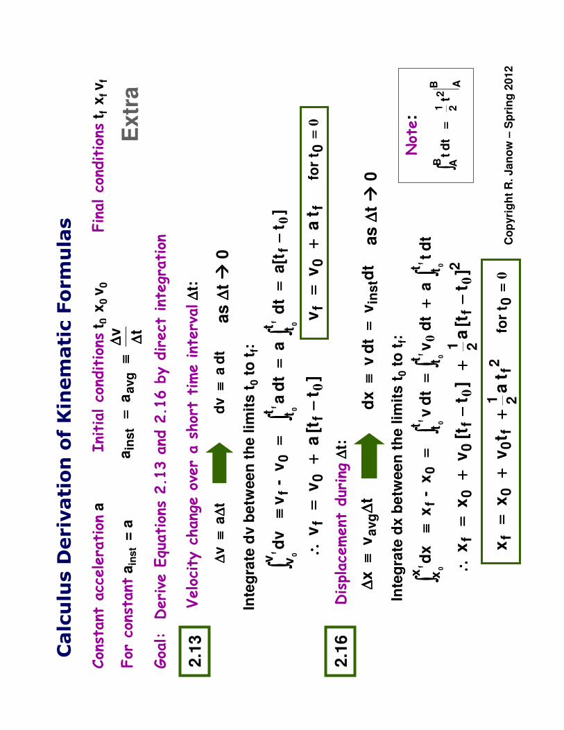
Calculus Derivation of Kinematic Formulas
Constant acceleration
a
Initial cond
itions
t 0 x
0 v
0Final cond
itions
t fx
fv
f
Goa
l: Derive Equations 2.13 and
2.16 by direct integration
tv
a
a
avg
inst
∆ ∆∆∆∆ ∆∆∆≡ ≡≡≡
= ===For constant
ain
st
= a
Velocity change over a short time interval
∆ ∆∆∆t:
ta
v
∆ ∆∆∆≡ ≡≡≡
∆ ∆∆∆t
d a
vd
≡ ≡≡≡
as ∆ ∆∆∆
t� ���
0
2.1
6
2.1
3
Inte
gra
te d
vb
etw
een
th
e l
imit
s t
0to
tf:
]t
a[t
dt
a
d
t
a
v -
v
v
d
ft t
t t0
fv v
f 0
f 0
f 0
0− −−−
= ==== ===
= ===≡ ≡≡≡
∫ ∫∫∫∫ ∫∫∫
∫ ∫∫∫
f0
f ]
t[t
a
v
v
0− −−−
+ +++= ===
∴ ∴∴∴
0t fo
rf
0f
t a
v
v
0= ===
+ +++= ===
Displacement during
∆ ∆∆∆t:
tv
x
avg
∆ ∆∆∆≡ ≡≡≡
∆ ∆∆∆d
tv
t
d
v
x
d
inst
= ===≡ ≡≡≡
as ∆ ∆∆∆
t� ���
0
Inte
gra
te d
xb
etw
een
th
e l
imit
s t
0to
tf:
d
tt
a
dt
v
dt
v
x
- x
x
d
f 0
f 0
f 0
f 0
t t
t t
t t0
fx x
∫ ∫∫∫∫ ∫∫∫
∫ ∫∫∫∫ ∫∫∫
+ +++= ===
= ===≡ ≡≡≡
0
Note:
B A
2
21B A
t
t
d t
= ===∫ ∫∫∫
2f
21
f0
0f
]t
[t a
]
t[t
v
x
x
00
− −−−+ +++
− −−−+ +++
= ===∴ ∴∴∴
0t
for
2 f21
f
00
f
t a
tv
x
x
0
= ===+ +++
+ +++= ===
Extr
a

Co
pyri
gh
t R
. J
an
ow
–S
pri
ng
2012
Kinematic Equations from Calculus
What if acceleration is NOT constant? V(t) graph is not a straight line
•The area und
er the
velocity-time graph
represents displacement
•Break graph
into rectangles
of w
idth ∆ ∆∆∆teach
•Each
rectangle has area: n
na
vg
nt
)
t(v
)t(
A∆ ∆∆∆
= ===∆ ∆∆∆
× ×××
•Add up all the area
rectangles from
tito t
f
if
xx
x− −−−
= ===∆ ∆∆∆
)t(
Ax
f it tn
∑ ∑∑∑∆ ∆∆∆
= ===∆ ∆∆∆
•The limit of the sum
is
a definite integral
∑ ∑∑∑∫ ∫∫∫
∑ ∑∑∑= ===
∆ ∆∆∆= ===
∆ ∆∆∆= ===
∆ ∆∆∆
→ →→→∆ ∆∆∆
→ →→→∆ ∆∆∆
f i
f i
f in
t t
t tt
t tn
tv(t
)dt
t)t(
v
Lim
)
t(A
L
imx
00
Extr
a
Top Related