


Languages
Pages
Legal


Copyright
by
Cody Ray Bond
2015

The Thesis Committee for Cody Ray Bond
Certifies that this is the approved version of the following thesis:
Mitigation of Municipal Biosolids via Conversion to Biocrude Oil Using
Hydrothermal Liquefaction: A Techno-economic Analysis
APPROVED BY
SUPERVISING COMMITTEE:
Halil Berberoglu
David Greene
Supervisor:
Mitigation of Municipal Biosolids via Conversion to Biocrude Oil Using
Hydrothermal Liquefaction: A Techno-economic Analysis
by
Cody Ray Bond, B.S.M.E
Thesis
Presented to the Faculty of the Graduate School of
The University of Texas at Austin
in Partial Fulfillment
of the Requirements
for the Degree of
Master of Science in Engineering
The University of Texas at Austin
May 2015

Dedication
Dedicated to my sister Deidra, for never being too busy to hear me complain or to exchange
cat videos.

v
Acknowledgements
This material is based upon work supported by the National Science Foundation
Graduate Research Fellowship under Grant No. DGE-1110007 and the National Science
Foundation Grant No. CBET-1254968. Any opinion, findings, and conclusions or
recommendations expressed in this material are those of the author and do not necessarily
reflect the views of the National Science Foundation.
I would like to thank my advisor Dr. Halil Berberoglu, David Greene, Jody Slagle
and the staff at HBBMP and Austin Water Utility, Environmental & Regulatory Services
for their help in providing plant data and expert insight. The project would not have been
as accurate or informative without them. Additionally, I would like to thank Jenny Kondo
for all of her administrative help over the last two years. She truly is the unsung hero of the
UT Mechanical Engineering department.
Finally, I would like to thank my lab members Joey Anthony, Daniel Campbell and
Daniel Pinero and my roommate, and dear friend, Robert Bush for keeping me sane and
making me feel like family.
vi
Abstract
Mitigation of Municipal Biosolids via Conversion to Biocrude Oil Using
Hydrothermal Liquefaction: A Techno-economic Analysis
Cody Ray Bond, M.S.E
The University of Texas at Austin, 2015
Supervisor: Halil Berberoglu
In this techno-economic analysis, we have shown that hydrothermal liquefaction
(HTL) technology can be integrated with existing biosolids management facilities that
utilize anaerobic digestion and biogas capture. The overall process converts raw sewage
sludge to refinery-ready biocrude oil. The Hornsby Bend Biosolids Management Plant
(HBBMP) in Austin, TX is used as a case study. First, the operation of the plant without
any modification was modeled and validated with field data. A standalone HTL processing
unit was then considered as an add-on to the existing infrastructure. Technical and
economic parameters were obtained from literature and experimental data. The results
showed that savings of about $32 M over current operation with a payback period of 4.35
years were achievable at HBBMP. A nation-wide implementation could result in
production of almost 4.5 million barrels of upgraded biocrude oil per year while offsetting
about 330,000 metric tons of CO2 equivalent greenhouse gas emissions annually.

vii
Table of Contents
Acknowledgements ..................................................................................................v
Abstract .................................................................................................................. vi
List of Tables ......................................................................................................... ix
List of Figures ..........................................................................................................x
Chapter 1 Introduction..........................................................................................1
1.1 Background and Motivation for the Study................................................1
1.2 Techno-economic Analysis .......................................................................3
1.3 Sensitivity Analysis ..................................................................................4
1.4 Organization of the Thesis ........................................................................5
Chapter 2 Mass & Energy Balance ......................................................................7
2.1 Analysis.....................................................................................................7
2.1.1 Base Case Scenario .......................................................................7
2.1.2 Case 1 Scenario ...........................................................................11
2.2 Results & Discussion ..............................................................................15
2.2.1 Model Validation ........................................................................15
2.2.2 Mass and Energy .........................................................................16
2.3 Sensitivity ...............................................................................................17
2.4 Conclusion ..............................................................................................19
Chapter 3 Economics ...........................................................................................20
3.1 Analysis...................................................................................................20
3.1.1 System Design ............................................................................20
3.1.2 Economic Calculations ...............................................................23
3.2 Results & Discussion ..............................................................................28
3.3 Sensitivity ...............................................................................................31
3.4 Conclusion ..............................................................................................35
Chapter 4 Greenhouse Gas Emissions ...............................................................36
4.1 Analysis...................................................................................................36

viii
4.2 Results & Discussion ..............................................................................40
4.3 Sensitivity ...............................................................................................45
4.4 Conclusion ..............................................................................................46
Chapter 5 Broader Impacts ................................................................................48
Chapter 6 Conclusion & Recommendations .....................................................50
6.1 Summary .................................................................................................50
6.2 Recommendations for Future Research ..................................................50
Appendices .............................................................................................................53
Appendix A: Nomenclature ..........................................................................54
Appendix B: Additional Mass & Energy Model Results .............................56
Appendix C: Additional Economic Model Results ......................................59
References ..............................................................................................................63
ix
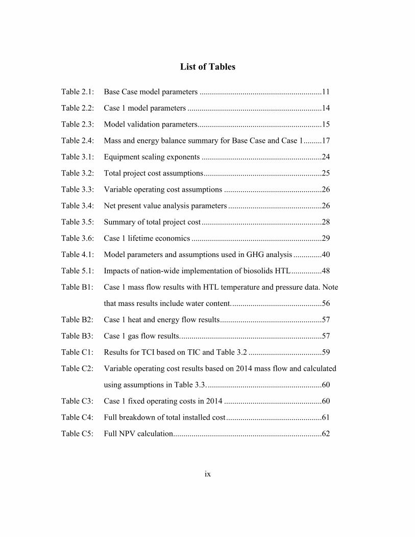
List of Tables
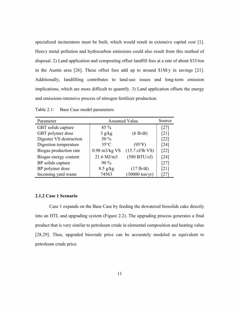
Table 2.1: Base Case model parameters ............................................................11
Table 2.2: Case 1 model parameters ..................................................................14
Table 2.3: Model validation parameters .............................................................15
Table 2.4: Mass and energy balance summary for Base Case and Case 1.........17
Table 3.1: Equipment scaling exponents ...........................................................24
Table 3.2: Total project cost assumptions ..........................................................25
Table 3.3: Variable operating cost assumptions ................................................26
Table 3.4: Net present value analysis parameters ..............................................26
Table 3.5: Summary of total project cost ...........................................................28
Table 3.6: Case 1 lifetime economics ................................................................29
Table 4.1: Model parameters and assumptions used in GHG analysis ..............40
Table 5.1: Impacts of nation-wide implementation of biosolids HTL ...............48
Table B1: Case 1 mass flow results with HTL temperature and pressure data. Note
that mass results include water content. ............................................56
Table B2: Case 1 heat and energy flow results ..................................................57
Table B3: Case 1 gas flow results. .....................................................................57
Table C1: Results for TCI based on TIC and Table 3.2 ....................................59
Table C2: Variable operating cost results based on 2014 mass flow and calculated
using assumptions in Table 3.3. ........................................................60
Table C3: Case 1 fixed operating costs in 2014 ................................................60
Table C4: Full breakdown of total installed cost ...............................................61
Table C5: Full NPV calculation.........................................................................62

x
List of Figures
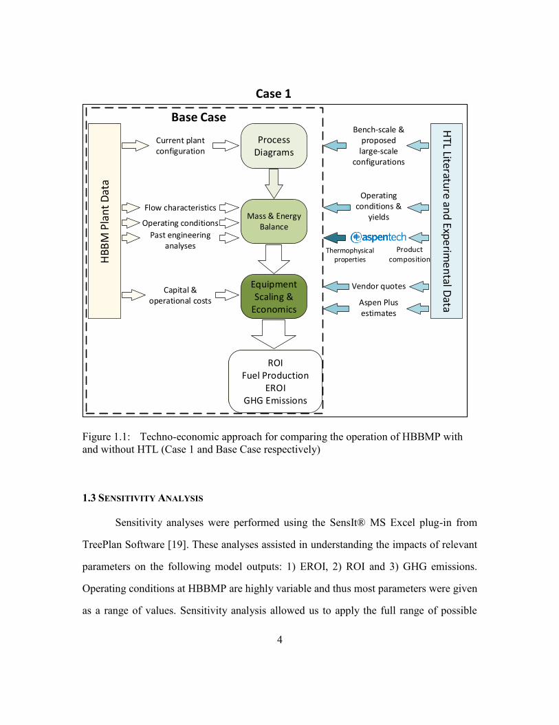
Figure 1.1: Techno-economic approach for comparing the operation of HBBMP
with and without HTL (Case 1 and Base Case respectively)..............4
Figure 2.1: Process flow diagram for Base Case scenario ....................................8
Figure 2.2: Process flow diagram for the Case 1 scenario ..................................12
Figure 2.3: Sensitivity of chosen parameters with regards to EROI ...................18
Figure 3.1: Heat exchanger nomenclature ...........................................................22
Figure 3.2: Variation of NPV across the life of the project.................................30
Figure 3.3: Sensitivity of chosen parameters with regards to ROI......................32
Figure 3.4: Two-factor sensitivity analysis results for ROI. The top six combinations
are reported in order of greatest increase in ROI. .............................34
Figure 4.1: GHG emissions boundaries with respect to business-as-usual. Biosolids
and petroleum fuel production do not affect one another, but both
generate GHGs. .................................................................................37
Figure 4.2: GHG emissions boundary for inclusion of the HTL system. The
biosolids and petroleum fuel systems become linked. ......................38
Figure 4.3: Comparison of GHG emissions per MJ of energy for gasoline
production via standard P2G and Case 1 ..........................................42
Figure 4.4: Comparison of GHG emissions per kg of incoming sludge between the
Base Case and Case 1 .......................................................................43
Figure 4.5: Total GHG emissions per year for BAU vs. Case 1. Despite an increase
in sludge treatment emissions at HBBMP, overall GHG emissions are
reduced by about 40%. ......................................................................44

xi
Figure 4.6: Sensitivity of selected parameters with regards to reduction in GHG
emissions of Case 1 compared to the P2G scenario. EISA RFS2 category
limits are shown by the gray dashed lines. .......................................45

1
Chapter 1
Introduction
1.1 BACKGROUND AND MOTIVATION FOR THE STUDY
Sewage sludge management is a growing, global problem. In the U.S. sewage
sludge is often converted to biosolids in accordance with federal and state regulation in
order to be re-used or properly disposed of [1]. The U.S. Environmental Protection
Agency (EPA) estimates that the U.S. alone currently produces over 8 million dry tons of
biosolids each year [2]. Approximately 40% of this is disposed of using expensive, non-
beneficial methods such as incineration and surface disposal [2]. Conversion of these waste
streams into biocrude oil would enable the production of an economically-valuable,
energetically-efficient product from what is typically a problem for biosolids management
facilities.
There are a wide variety of bio- and thermochemical processes that can be used to
synthesize biofuels. In this study we focused on hydrothermal liquefaction (HTL), which
is a thermochemical process that takes advantage of the reactive, subcritical properties of
water to convert biomass into a liquid fuel. In its subcritical stage, water acts as a catalyst
and reactant, which allows for direct conversion of biomass without the need for
energetically-intensive drying steps seen in other biofuel processes [3]. The sludge and
biosolids waste streams already exist in slurry form, requiring little to no additional
preparation prior to HTL processing.
The literature and our own experiments show that pre- and post-digested sludge, as
well as farm-generated manure, are viable feedstocks for HTL [3–5]. It has also been shown
that HTL can mitigate the environmental impacts of sludge and biosolids disposal by: 1)
significantly reducing the heavy metal leaching rates and ecological risk index of all HTL
2
products, and 2) removing pathogens using the high processing temperature [6]. The liquid
fuel product of HTL is commonly referred to as biocrude. Compared to petroleum crude,
biocrude differs mostly in its elevated nitrogen and oxygen contents [3,5,7,8]. This requires
that the biocrude be hydro-treated prior to refining [7,9]. Once treated the biocrude can
serve as a petroleum crude blendstock without significant refinery infrastructure changes
[10].
Additionally, products refined from biocrude may be considered under the Energy
Independence and Security Act of 2007 (EISA) and the updated Renewable Fuel Standard
(RFS2). This policy mandates yearly, minimum biofuel usage standards in the US,
increasing to 36 billion gallons by 2022 [11–13]. Currently the most common and widely
produced biofuel is corn-based ethanol, of which the advantages and disadvantages are
environmentally and politically debated. Converting waste streams such as sludge, manure
and biosolids into biofuel could help meet this biofuel standard by contributing to national
energy independence and reduced greenhouse gas (GHG) emissions, while also reducing
valuable land usage and diversion of food crops.
The purpose of this study was to evaluate the economic and energetic feasibility of
integrating an HTL pathway to existing biosolids production plant infrastructure. The
techno-economic (TE) model was built on an assembly of published, experimental and
economic HTL data, current operational data from Hornsby Bend Biosolids Management
Plant (HBBMP) and thermodynamic property data from Aspentech’s Aspen Plus modeling
software [14]. This study also considered environmental impacts and sustainability of the
proposed production pathway.

3
1.2 TECHNO-ECONOMIC ANALYSIS
Figure 1.1 presents the framework for the TE analysis that is utilized in this study.
TE analysis is a strategy that integrates process modeling, mass and energy balances,
economic factors and environmental sustainability into a single report. This enables both
effective comparison of technologies and design and optimization of processes to meet
economic, energetic and environmental targets.
One approach in evaluating emerging renewable fuel technologies via TE analysis
is to incorporate a discounted cash flow analysis in order to calculate a minimum fuel
selling price [15–18]. Alternatively, this study leveraged a net present value (NPV)
approach in order to compare current operation at HBBMP (Base Case) to the proposed
case where HTL is incorporated into the existing infrastructure (Case 1). The goal was for
the model to predict return on investment (ROI), pay-back time, energy return on energy
investment (EROI), fuel production, environmental impact and sustainability.
4
Process Diagrams
Mass & Energy Balance
Equipment Scaling &
Economics
ROIFuel Production
EROIGHG Emissions
HTL Literatu
re and
Expe
rime
ntal D
ataBase Case
Case 1
Current plant configuration
Bench-scale & proposed
large-scale configurations
Product composition
Thermophysical properties
Operating conditions &
yields
Capital & operational costs
Vendor quotes
Aspen Plus estimates
Flow characteristics
Operating conditions
Past engineering analyses
HB
BM
Pla
nt
Dat
a
Figure 1.1: Techno-economic approach for comparing the operation of HBBMP with
and without HTL (Case 1 and Base Case respectively)
1.3 SENSITIVITY ANALYSIS
Sensitivity analyses were performed using the SensIt® MS Excel plug-in from
TreePlan Software [19]. These analyses assisted in understanding the impacts of relevant
parameters on the following model outputs: 1) EROI, 2) ROI and 3) GHG emissions.
Operating conditions at HBBMP are highly variable and thus most parameters were given
as a range of values. Sensitivity analysis allowed us to apply the full range of possible

5
values and identify which parameters affected the final outcomes the most and in what
way. Sensitivity reporting was especially important with regards to the significant
uncertainty associated with parameters such as crude oil price and discount and tax rates.
Two-factor sensitivity was also performed. This analysis compiles all possible
combinations of parameters to show the sensitivity of varying two parameters
simultaneously. Results from a two-factor sensitivity analysis can make it easier to realize
the full potential of projects based on unproven technology. Two-factor analysis is most
beneficial for projects in which multiple parameter adjustments are realistic, or for multiple
parameters that are expected to change with time, such as crude oil price and federal tax
rates.
1.4 ORGANIZATION OF THE THESIS
Chapter 2 of this study begins with process modeling and mass and energy
balances, which were the core of the overall analysis. This chapter includes full process
diagrams of both cases. Model validation was performed in comparison to current plant
data and past City of Austin (CoA) reports and data. Results of this chapter include
estimated fuel production, energy consumption, EROI and a sensitivity analysis.
Chapter 3 presents work which utilized the mass and energy balance results from
Chapter 2 to estimate economic parameters.1 The design of the HTL and upgrading systems
are discussed in terms of individual component cost, scaling and adjustment. Major
equations and assumptions are included. The results of Chapter 3 include ROI, pay-back
1 Results, findings, opinions and recommendations presented by the authors in Chapter 3 should not be
used for investment purposes without further study and understanding of associated uncertainties. This
study should be used for estimation purposes only.

6
time and total capital investment. Single and two-parameter sensitivity analyses were
performed with respect to ROI.
Chapter 4 continues the TE analysis by estimating environmental impact from GHG
emissions. Three GHG analyses were performed. The first analysis compared sludge HTL
emissions to those of petroleum-derived gasoline. The second compared sludge HTL to
current operation at HBBMP as a biosolids mitigation strategy in terms of local GHG
impact. The third analysis compared sludge HTL to the business-as-usual case where
HBBMP and gasoline production emit GHGs simultaneously.
Analysis performed in Chapter 5 utilizes the mass balance and GHG emissions
models described in Chapters 2 and 4, respectively, to estimate the impact of nation-wide
sludge HTL implementation. These results presented in this chapter give a high-level
estimate of the future potential of sludge HTL as a fuel producer.
Finally, Chapter 6 includes a discussion on the overall project summary and
possible future studies that would benefit sludge HTL technology.
7
Chapter 2
Mass & Energy Balance
2.1 ANALYSIS
2.1.1 Base Case Scenario
Microsoft Excel 2013 was used to construct a model that characterizes yearly-
averaged, typical operation of HBBMP. We referred to this scenario as the Base Case. The
Base Case was built from and validated by process data and engineering reports provided
to us by the staff at HBBMP and Environmental & Regulatory Services, both of which are
a part of the Austin Water Utility (AWU). Table 2.1, at the end of this section, presents a
summary of the operational parameters used for the Base Case scenario.
Figure 2.1 shows the schematic of the current processes for managing sewage
sludge and biosolids at HBBMP. The plant processes two main sludge flows which are a
mixture of primary and secondary activated sludge from AWU’s two main wastewater
treatment plants: South Austin Regional (SAR) Wastewater Treatment Plant (WWTP) and
Walnut Creek (WC) WWTP. These incoming streams were not included in model
calculations due to uncertainty from only having a single month of data. In May 2014,
SAR contributed approximately 0.689 million gallons per day (MGD) at 2% total solids
(TS) and WC contributed approximately 0.7 MGD at 2.6% TS [20]. A third stream from
the on-site water treatment facility contributed about 0.04 MGD at 2% TS. This smaller
stream is made up of recovered solids from the various thickening and dewatering
processes in the main plant [20,21].

8
Figure 2.1: Process flow diagram for Base Case scenario
Po
lym
er(P
1)
Gra
vity
Be
ltTh
icke
ne
r
W1
An
aero
bic
Dig
esti
on
4B
iog
asB
oile
r
On
-Sit
e Se
con
dar
yTr
eat
me
nt
Be
lt P
ress
23
Po
lym
er(P
2)
Co
-ge
ne
rati
on
G2
H1
G4
E2
56
W2
E4
W4
Slu
dge
He
atin
gLo
op
H2
E3
Infl
ue
nt
Co
mp
ost
9
Yard
Wa
ste
(YW
)
10
Dill
oD
irt©
Flo
w E
qu
aliz
atio
n
Ba
sin
1b
Scre
en
ing
1a
Sou
th A
ust
in
Re
gio
na
lW
aln
ut
Cre
ek
Lan
d A
pp
licat
ion
8
7
1c
G1
Flar
e
W3
Hol
din
g Po
nd
s
E1
E5
BO
P
Con
trac
t Co
mp
ost
11
Solid
s
He
at
Ele
ctri
city
Wat
er
Ga
sG
3
E6G
rid

9
The two main streams from SAR and WC are screened for large objects, such as
storm debris and garbage, and then combine with the recycle stream in a flow equalization
basin (FEB), which serves to damp the variation in the incoming flow rates and provide a
steady effluent flow [22]. The FEB also serves as the input to the model due to frequent
flow measurements made there. After leaving the FEB, a cationic polyelectrolyte is added
to the stream at a rate of about 5-10 lb/dry ton of solids (dt) [21,23]. This polymer causes
flocculation of the solid particles and increases the efficiency of the gravity belt thickeners
(GBT). The GBTs concentrate the flow to approximately 7% TS where it is then pumped
to the anaerobic digesters.
The HBBMP digester complex is comprised of eight digesters, each with a capacity
of 2 MG. The digestion process creates two products: 1) biogas from the organic
breakdown of volatile solids (VS), and 2) Class B biosolids at approximately 5% TS [20].
Biogas from anaerobic digestion is generated at a rate of about 0.75-1.12 m3/(kg-VS
destroyed) and is typically composed of approximately 62% methane and 35% carbon
dioxide on average [20,22]. This composition contains an energy content of approximately
20.5-22.4 MJ/m3 (570-620 BTU/cf) [24]. This is compared to about 39 MJ/m3 (1000
BTU/cf) for natural gas [24]. Digester gas also commonly contains hydrogen sulfide (H2S),
moisture and siloxanes [22,24]. HBBMP actively removes H2S and siloxanes prior to
combustion due to their corrosive and abrasive properties [21]. The majority of the
generated biogas is used to fuel a single GE Jenbacher Type 3 cogeneration (co-gen) unit.
The remaining biogas is either sent to boilers to produce additional heat, or flared off in
order to reduce GHG emissions.
The co-gen is capable of generating a maximum 848 kWe/1118 kWt and supplies
all of the electricity needed to run the plant, via net-metering with the grid, and the heat
needed to sustain digestion temperatures of 35°C for most of the year [25]. During the
10
winter months additional heat is supplied by the biogas boilers at a rate of about 3500 GJ/hr
via hot water-loop heat exchangers [24]. Class B biosolids are discharged after an
approximately 30 day residence time and then pumped to the belt presses (BP) where
additional polymer is added for further dewatering [21]. The dewatered biosolids, referred
to as “cake,” are then divided into three product streams: 1) land application, 2) contract
composting, and 3) Dillo Dirt™ production.
In general, the quality of biosolids material is divided into two pathogen density
levels, Class A and B, according to the EPA Title 40 CFR Part 503 [1]. Class B is the
minimum requirement for land application, surface disposal and incineration. HBBMP
biosolids meet Class B requirements through the anaerobic digestion process. At HBBMP
about 50% of biosolids production, by volume, is used as agricultural land application [21].
The other half of the biosolids material is combined with approximately 75 MT/d of city-
generated yard waste in order to be composted.
Composting is considered by the CFR as a pathway to achieve Class A biosolids
status [1]. Approximately half of the HBBMP compost stream is managed by contractors
and the other half is used by HBBMP to produce Dillo Dirt, which is an EPA-certified,
Class A compost that is used in parks and gardens around the City of Austin. There are no
restrictions on its application.
All three product streams are produced at a monetary net loss when capital and
fixed costs are considered, which is standard for biosolids management plants [21]. Dillo
Dirt is the most monetarily attractive output for the Base Case scenario due to having the
lowest net production cost.
Despite a monetary loss, HBBMP offsets many other costs and additional benefits
are gained in the following ways: 1) Land application directly offsets solid waste that
would otherwise be incinerated or sent to surface disposal. In order to incinerate the waste,
11
specialized incinerators must be built, which would result in extensive capital cost [1].
Heavy metal pollution and hydrocarbon emissions could also result from this method of
disposal. 2) Land application and composting offset landfill fees at a rate of about $33/ton
in the Austin area [26]. These offset fees add up to around $1M/y in savings [21].
Additionally, landfilling contributes to land-use issues and long-term emission
implications, which are more difficult to quantify. 3) Land application offsets the energy
and emissions-intensive process of nitrogen fertilizer production.
Table 2.1: Base Case model parameters
Parameter Assumed Value Source
GBT solids capture 85 % [27]
GBT polymer dose 3 g/kg (6 lb/dt) [21]
Digester VS destruction 50 % [22]
Digestion temperature 35°C (95°F) [24]
Biogas production rate 0.98 m3/kg VS (15.7 cf/lb VS) [22]
Biogas energy content 21.6 MJ/m3 (580 BTU/cf) [24]
BP solids capture 90 % [27]
BP polymer dose 8.5 g/kg (17 lb/dt) [21]
Incoming yard waste 74563 (30000 ton/yr) [27]
2.1.2 Case 1 Scenario
Case 1 expands on the Base Case by feeding the dewatered biosolids cake directly
into an HTL and upgrading system (Figure 2.2). The upgrading process generates a final
product that is very similar to petroleum crude in elemental composition and heating value
[28,29]. Thus, upgraded biocrude price can be accurately modeled as equivalent to
petroleum crude price.

12
Figure 2.2: Process flow diagram for the Case 1 scenario
Solid
s
He
at
Ele
ctri
city
Wat
er
Ga
s
Bio
solid
s Pr
od
uct
s
8, 1
0, 1
1H
igh
Pre
ssu
reP
um
p
HT
LR
eac
tor
Solid
sFi
lter
H3
19
17
14
Pre
he
at1
5
16
Sep
arat
or
G5
18
Ch
ar
13
E7
W5
P1
Gra
vity
Be
ltTh
icke
ne
r
W1
An
aero
bic
Dig
esti
on
4
Bio
gas
Bo
iler
On
-Sit
e Se
con
dar
yTr
eat
me
nt
Be
lt P
ress
23
P2
Co
-ge
ne
rati
on
G2
H1
G4
E2
5
6
W2
E4
W4
H2
E3
Infl
uen
t
Flo
w E
qu
aliz
atio
n
Ba
sin
1b
Scre
en
ing
1a
Sou
th A
ust
in
Re
gio
na
l
Wal
nu
t C
ree
k
71
c
G1
Flar
e
W3
Hol
din
g P
on
ds
E1
E5
BO
PE
6
Gri
d
G3
12
Off
-Gas
Aq
ueo
us
Hyd
rotr
eat
er
G6
20
Up
grad
edB
iocr
ud
eW
6G
8G7
W7 G
9
H4
E8H
TL S
yste
mU
pgr
adin
g
13
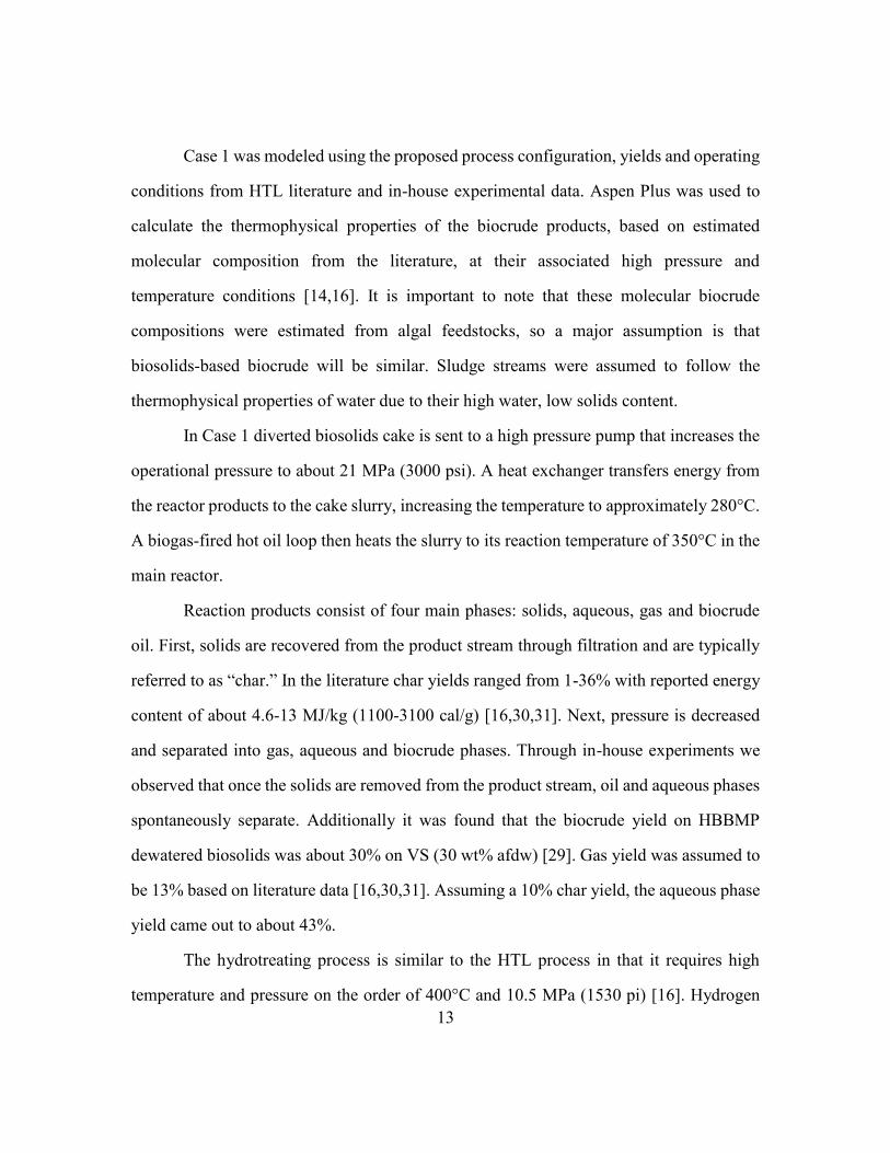
Case 1 was modeled using the proposed process configuration, yields and operating
conditions from HTL literature and in-house experimental data. Aspen Plus was used to
calculate the thermophysical properties of the biocrude products, based on estimated
molecular composition from the literature, at their associated high pressure and
temperature conditions [14,16]. It is important to note that these molecular biocrude
compositions were estimated from algal feedstocks, so a major assumption is that
biosolids-based biocrude will be similar. Sludge streams were assumed to follow the
thermophysical properties of water due to their high water, low solids content.
In Case 1 diverted biosolids cake is sent to a high pressure pump that increases the
operational pressure to about 21 MPa (3000 psi). A heat exchanger transfers energy from
the reactor products to the cake slurry, increasing the temperature to approximately 280°C.
A biogas-fired hot oil loop then heats the slurry to its reaction temperature of 350°C in the
main reactor.
Reaction products consist of four main phases: solids, aqueous, gas and biocrude
oil. First, solids are recovered from the product stream through filtration and are typically
referred to as “char.” In the literature char yields ranged from 1-36% with reported energy
content of about 4.6-13 MJ/kg (1100-3100 cal/g) [16,30,31]. Next, pressure is decreased
and separated into gas, aqueous and biocrude phases. Through in-house experiments we
observed that once the solids are removed from the product stream, oil and aqueous phases
spontaneously separate. Additionally it was found that the biocrude yield on HBBMP
dewatered biosolids was about 30% on VS (30 wt% afdw) [29]. Gas yield was assumed to
be 13% based on literature data [16,30,31]. Assuming a 10% char yield, the aqueous phase
yield came out to about 43%.
The hydrotreating process is similar to the HTL process in that it requires high
temperature and pressure on the order of 400°C and 10.5 MPa (1530 pi) [16]. Hydrogen

14
gas and cobalt-molybdenum catalyst are needed in order to remove nitrogen and oxygen
from the oil. The overall process was simplified to a single block in Figure 2.2. Within this
block, pressure is maintained from HTL separation conditions and hydrogen gas is added
at a rate of 0.05 kg H2/kg biocrude [7,16,31]. The hydrogen is assumed to be delivered
periodically by truck and stored in a pressurized tank on-site. The biocrude oil is then
pumped through a heat exchanger with the hydrotreated products, increasing the
temperature to approximately 171°C. Then, the biocrude oil comes into contact with the
catalyst and is heated to the process temperature of 400°C in the main reactor. Excess
hydrogen is captured and recycled. Upgraded biocrude was assumed to be produced at a
yield rate of 80% [4,16,18].
Table 2.2: Case 1 model parameters
Parameter Assumed Value Source
HTL reactor temperature 350°C (662°F) [16,17]
HTL reactor pressure 20684 kPa (3000 psi) [16,17]
Biocrude yield 30 wt% afdw [29]
Cake heat capacity 4.187 kJ/kg-K
Upgrading temperature 400°C (752°F) [16]
Upgrading pressure 10549 kPa (1530 psi) [16]
H2 feed rate 0.05 kg/kg biocrude [4,16,18]
Catalyst loading 0.625 wt/hr per wt
catalyst [16]
Upgrade yield 80 % [4,16,18]
Upgraded biocrude density
(@40°C) 0.78 kg/L (6.5 lb/gal) [28]

15
2.2 RESULTS & DISCUSSION
2.2.1 Model Validation
Base Case results were validated with values interpolated from HBBMP flow
projections reported by the CoA, which are summarized in Table 2.3. The flow points in
Table 2.3 were chosen due to their availability in the report as well as their energetic and
economic importance. In particular the mass of dewatered cake from the BP was chosen
because it is the output for the Base Case and the material link between the Base Case and
Case 1.
Table 2.3: Model validation parameters
Parameter 2012a 2030a 2014b Base Case Difference
FEB effluent [dt/d] 92 147 98 99c 0.6%
Dewatered cake [dt/d] 54 87 58 55 4.4%
Biogas [mmcf/d] 0.85 1.35 0.91 0.89 1.5%
GBT polymer [ton/y] 100 162 107 108 0.8%
BP polymer [ton/y] 175 284 187 190 1.7% aProjected from 2009 [32] bBy linear interpolation cMeasured value [21]
Overall, the model showed less than 5% difference in mass flow compared to the
CoA reported projections, with a span of 0.6-4.4%. The lowest difference was the FEB
effluent, which was the input to the model. Sludge production is a function of city
population, which typically increases linearly across time. Thus, uncertainty should be low
with regards to the flow estimates. The highest difference was with the cake output. This
was expected due to the number of systems and assumptions made between the input and
output. HBBMP has also been in an almost constant state of upgrading and retrofitting for
the last few years [21]. This increases uncertainty in digester and dewatering performance

16
assumptions. A maximum difference of less than 5% was deemed acceptable to ensure
accuracy of the flow moving forward to Case 1.
2.2.2 Mass and Energy
Total output was about 6.9 MT/d (55 bbl/d) of upgraded biocrude oil and 2.7 MT/d
of solid char for Case 1 in 2014 (Table 2.4). These amounts were a result of the economic
optimization of the model for maximum daily production value, which is described in
Section 3.1.1. This optimization resulted in 100% of the biosolids cake being diverted to
HTL. The initial inputs to the model were the FEB effluent flow, TS and VS content. The
yearly-averaged flow at this point was measured from October 2013 – September 2014 to
be about 89.5 dry MT/d (98.7 dtpd) [21]. From this input the model reports about 50 dry
MT/d (55 dtpd) of biosolids output at the BP that was then fed into the HTL system.
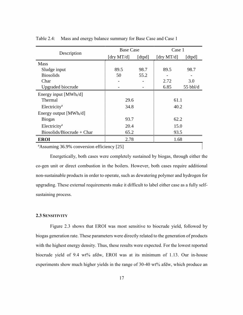
Table 2.4 reports the mass and energy balance results, as well as EROI for the Base
Case and Case 1. EROI was calculated simply as total energy output divided by total energy
input. The Base Case and Case 1 EROIs were calculated to be 2.78 and 1.68 respectively.
Energy outputs were considered to be biosolids cake for the Base Case, upgraded biocrude
oil and char for Case 1 and excess biogas energy and electricity for both cases. Electric
energy was converted to its thermal energy equivalent using the efficiency of the co-gen.
In the Base Case only 48% of biogas by volume was utilized. This large amount of excess
energy accounts for the greater Base Case EROI. Complete mass and energy balance
results can be found in Appendix B.
17
Table 2.4: Mass and energy balance summary for Base Case and Case 1
Description Base Case Case 1
[dry MT/d] [dtpd] [dry MT/d] [dtpd]
Mass
Sludge input 89.5 98.7 89.5 98.7
Biosolids 50 55.2 - -
Char - - 2.72 3.0
Upgraded biocrude - - 6.85 55 bbl/d
Energy input [MWht/d]
Thermal 29.6 61.1
Electricitya 34.8 40.2
Energy output [MWht/d]
Biogas 93.7 62.2
Electricitya 20.4 15.0
Biosolids/Biocrude + Char 65.2 93.5
EROI 2.78 1.68
aAssuming 36.9% conversion efficiency [25]
Energetically, both cases were completely sustained by biogas, through either the
co-gen unit or direct combustion in the boilers. However, both cases require additional
non-sustainable products in order to operate, such as dewatering polymer and hydrogen for
upgrading. These external requirements make it difficult to label either case as a fully self-
sustaining process.
2.3 SENSITIVITY
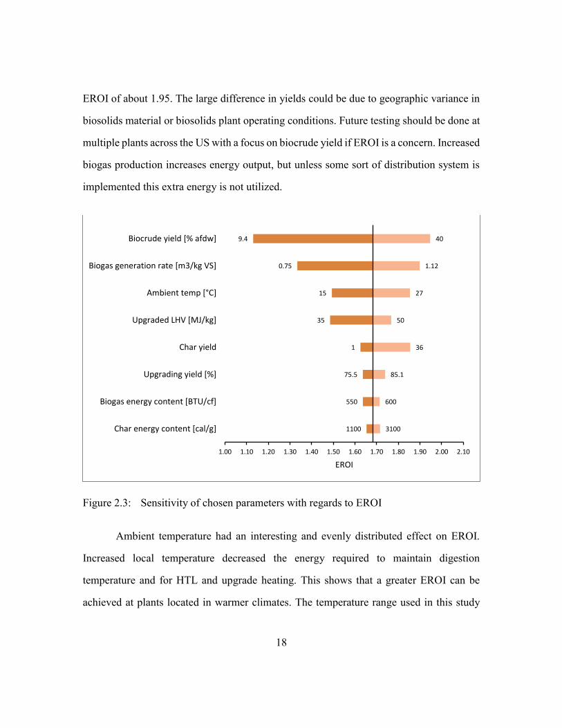
Figure 2.3 shows that EROI was most sensitive to biocrude yield, followed by
biogas generation rate. These parameters were directly related to the generation of products
with the highest energy density. Thus, these results were expected. For the lowest reported
biocrude yield of 9.4 wt% afdw, EROI was at its minimum of 1.13. Our in-house
experiments show much higher yields in the range of 30-40 wt% afdw, which produce an
18
EROI of about 1.95. The large difference in yields could be due to geographic variance in
biosolids material or biosolids plant operating conditions. Future testing should be done at
multiple plants across the US with a focus on biocrude yield if EROI is a concern. Increased
biogas production increases energy output, but unless some sort of distribution system is
implemented this extra energy is not utilized.
Figure 2.3: Sensitivity of chosen parameters with regards to EROI
Ambient temperature had an interesting and evenly distributed effect on EROI.
Increased local temperature decreased the energy required to maintain digestion
temperature and for HTL and upgrade heating. This shows that a greater EROI can be
achieved at plants located in warmer climates. The temperature range used in this study
9.4
0.75
15
35
1
75.5
550
1100
40
1.12
27
50
36
85.1
600
3100
1.00 1.10 1.20 1.30 1.40 1.50 1.60 1.70 1.80 1.90 2.00 2.10
Biocrude yield [% afdw]
Biogas generation rate [m3/kg VS]
Ambient temp [°C]
Upgraded LHV [MJ/kg]
Char yield
Upgrading yield [%]
Biogas energy content [BTU/cf]
Char energy content [cal/g]
EROI

19
was the span of local, yearly-averaged high and low temperatures [33]. This also shows
that the EROI should be expected to fluctuate between about 1.5 and 1.85 annually.
2.4 CONCLUSION
Overall we see that the model produces relatively accurate results in terms of mass
flow. Mass flow is very important because all proceeding analyses depend on it. Case 1
was found to be sustainable with regard to energy requirements, but only semi-sustainable
overall due to required external inputs such as dewatering polymer and hydrogen. Case 1
was able to produce 55 bbl/d of upgraded biocrude oil based on current biosolids
production rate. Going forward this production rate will increase with increasing sludge
input.
An EROI of 1.68 is favorable when compared to other biofuel pathways. As
reported by Liu et al., cellulosic and corn ethanol were calculated to have EROIs of around
1 and slightly less than 1, respectively [34]. In the same study, the Sapphire pilot-scale,
algal HTL plant operating in southern New Mexico was found to have an EROI of slightly
less than 1. Our sensitivity analysis shows that, based on changes to a single parameter,
Case 1 EROI could be as low as about 1.1 and as high as about 2.

20
Chapter 3
Economics
3.1 ANALYSIS
3.1.1 System Design
Process economics were separated into two main systems: the HTL system and the
upgrading system. The HTL system considered in this study was largely based on Case D
as reported by Knorr et al. [31]. This case was chosen for its simplistic design,
consideration of high-solids content feedstock (up to 36.6 wt%) and shell and tube heat
exchangers. Costs were broken down by individual component, which allowed us to
consider only those needed for sludge HTL.
The upgrading system was based on that reported by Jones et al. [16], which was
constructed to handle algal biocrude all the way through to its constituent biofuels of
gasoline, diesel and jet fuel. The components in this system are simply smaller versions of
those found in a petroleum refinery. Ultimately the upgrading process would be executed
at an existing petroleum refinery. For that to happen, refineries would need to be able to
accept raw biocrude oil, at which point it would be assigned a market value. Economic
analyses would then not need to consider on-site upgrading and would instead use the
market value for untreated biocrude oil.
Cooling and storage systems were also considered in the overall process cost,
similar to that reported by Jones et al. [16]. A cooling system is needed in order to bring
most of the process streams back to ambient conditions. Storage is needed due to the
relatively low production volume and to enable less frequent, higher capacity freight.
Full scale HTL plants from the literature have a capacity of about 1300-2000 dry
tons of feedstock per day, which is achieved with 2-4 parallel reactor trains [16,31]. In this
21
study the HTL system was sized to handle a mass flow rate on the order of 300 dry tons
per day, which corresponds to the projected, maximum week flow at HBBMP in 2034 [32].
This year was chosen based on an assumed 20 year life. In order to utilize the associated
literature data, these systems must be scaled down. Economic scaling is most effective at
the component level since different pieces of equipment scale in different ways. These
calculations are addressed in Section 3.1.2.
Special consideration was paid to the heat exchangers in the HTL system. This was
due to their complicated construction, high cost and energetic importance. According to
Knorr et al., the high cost is largely attributed to the size and extreme design pressure of
greater than 3000 psi. Most fabricators are only ASTM-certified up to 3000 psi, and beyond
that would need to be qualified for a different stamp. This creates a relatively small pool
of fabricators that can complete the work, thus raising the overall cost. [31]
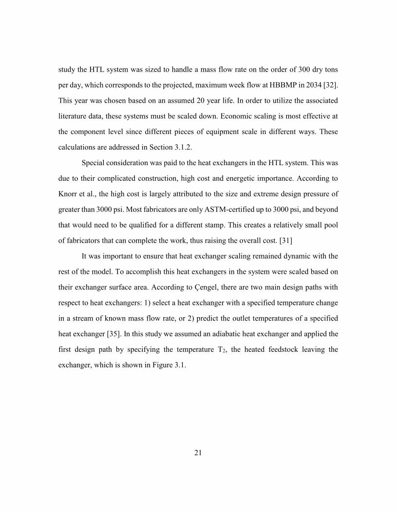
It was important to ensure that heat exchanger scaling remained dynamic with the
rest of the model. To accomplish this heat exchangers in the system were scaled based on
their exchanger surface area. According to Çengel, there are two main design paths with
respect to heat exchangers: 1) select a heat exchanger with a specified temperature change
in a stream of known mass flow rate, or 2) predict the outlet temperatures of a specified
heat exchanger [35]. In this study we assumed an adiabatic heat exchanger and applied the
first design path by specifying the temperature T2, the heated feedstock leaving the
exchanger, which is shown in Figure 3.1.

22
T2
T3T4
T1
To HTL reactor
From HTL reactor
From HP pump
To solids filter
Figure 3.1: Heat exchanger nomenclature
In order to calculate heat exchanger surface area, the heat transfer rate (�̇�), overall
heat transfer coefficient (𝑈) and temperature difference must be known. This study used
the log mean temperature difference method, which is defined according to [35],
�̇� = 𝑈𝐴 (
∆𝑇2,3 − ∆𝑇1,4
ln (∆𝑇2,3
∆𝑇1,4)
) (1)
The heat transfer rate was related to the mass flow rate and change in enthalpy of
the fluid according to [35],
�̇� = �̇�∆ℎ (2)
The overall heat transfer coefficient was thoroughly investigated by Knorr et al.,
and the coefficients from the appropriate case in that study were used here [31]. The base
values of 170 and 154 BTU/hr/ft2/°F were used for the preheating and hot oil heat
exchangers, respectively.
As discussed earlier sludge streams were assumed to mimic the thermal properties
of water as they ranged from 80-99% water by mass. Thus, enthalpy values were estimated
as those of water and obtained from the National Institute of Standards and Technology
23
(NIST) Thermophysical Properties of Fluid Systems web model at the specified
temperatures and pressures [36]. Enthalpies for biocrude and upgraded biocrude were
found using Aspen Plus according to their estimated molecular composition [14,16].
Case 1 was optimized for maximum production value by varying the amount of
biosolids that went to the following outputs: 1) HTL, 2) Dillo Dirt, 3) contract composting
and 4) land application. This optimization was performed with the Evolutionary solving
method that is built in to Excel. This method was chosen for its ability to handle nonlinear
and non-smooth nonlinear functions, which are embedded in the model. The optimization
begins with an output distribution identical to the Base Case. Then as the mass flow rate of
biosolids cake is diverted to the HTL process, mass flow rate is deducted first from land
application, then from contract composting and finally from Dillo Dirt. In this way, mass
is diverted in order from the most expensive to least expensive products and converted to
the high-value, upgraded biocrude product.
3.1.2 Economic Calculations
In order to determine pay-back time and return on investment (ROI), yearly net
cash flow (NCF) and total capital investment (TCI) must be calculated. Pay-back time is
the amount of time required to earn a profit equal to that of the investment. ROI is the ratio
of total project earnings to project cost, or in this case the ratio of NPV to capital cost. Once
NCF and TCI were found, the NPV analysis was performed to estimate the ROI.
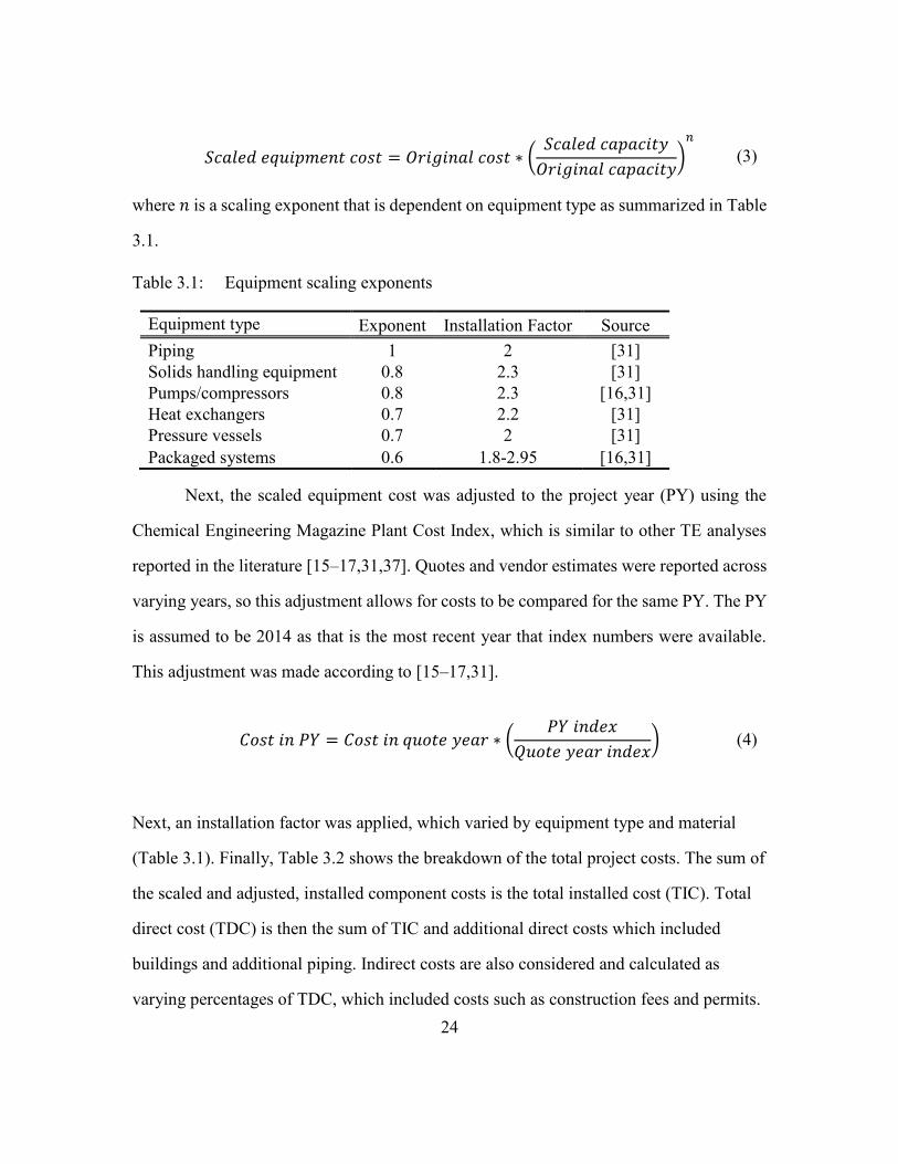
First, each component was scaled according to appropriate scaling variables, which
included volumetric flow rate for pumps, surface area for heat exchangers and length for
piping. Cost was then scaled according to [15–17,31],
24
𝑆𝑐𝑎𝑙𝑒𝑑 𝑒𝑞𝑢𝑖𝑝𝑚𝑒𝑛𝑡 𝑐𝑜𝑠𝑡 = 𝑂𝑟𝑖𝑔𝑖𝑛𝑎𝑙 𝑐𝑜𝑠𝑡 ∗ (𝑆𝑐𝑎𝑙𝑒𝑑 𝑐𝑎𝑝𝑎𝑐𝑖𝑡𝑦
𝑂𝑟𝑖𝑔𝑖𝑛𝑎𝑙 𝑐𝑎𝑝𝑎𝑐𝑖𝑡𝑦)
𝑛
(3)
where 𝑛 is a scaling exponent that is dependent on equipment type as summarized in Table
3.1.
Table 3.1: Equipment scaling exponents
Equipment type Exponent Installation Factor Source
Piping 1 2 [31]
Solids handling equipment 0.8 2.3 [31]
Pumps/compressors 0.8 2.3 [16,31]
Heat exchangers 0.7 2.2 [31]
Pressure vessels 0.7 2 [31]
Packaged systems 0.6 1.8-2.95 [16,31]
Next, the scaled equipment cost was adjusted to the project year (PY) using the
Chemical Engineering Magazine Plant Cost Index, which is similar to other TE analyses
reported in the literature [15–17,31,37]. Quotes and vendor estimates were reported across
varying years, so this adjustment allows for costs to be compared for the same PY. The PY
is assumed to be 2014 as that is the most recent year that index numbers were available.
This adjustment was made according to [15–17,31].
𝐶𝑜𝑠𝑡 𝑖𝑛 𝑃𝑌 = 𝐶𝑜𝑠𝑡 𝑖𝑛 𝑞𝑢𝑜𝑡𝑒 𝑦𝑒𝑎𝑟 ∗ (𝑃𝑌 𝑖𝑛𝑑𝑒𝑥
𝑄𝑢𝑜𝑡𝑒 𝑦𝑒𝑎𝑟 𝑖𝑛𝑑𝑒𝑥) (4)
Next, an installation factor was applied, which varied by equipment type and material
(Table 3.1). Finally, Table 3.2 shows the breakdown of the total project costs. The sum of
the scaled and adjusted, installed component costs is the total installed cost (TIC). Total
direct cost (TDC) is then the sum of TIC and additional direct costs which included
buildings and additional piping. Indirect costs are also considered and calculated as
varying percentages of TDC, which included costs such as construction fees and permits.

25
Fixed capital investment (FCI) is the sum of TDC and indirect costs. Finally, total capital
investment is the sum of FCI and working capital which can be written as,
𝑇𝐶𝐼 = [(𝑇𝐼𝐶 + 𝐷𝑖𝑟𝑒𝑐𝑡 𝑐𝑜𝑠𝑡𝑠)𝑇𝐷𝐶 + 𝐼𝑛𝑑𝑖𝑟𝑒𝑐𝑡 𝑐𝑜𝑠𝑡𝑠]𝐹𝐶𝐼 + 𝑊𝑜𝑟𝑘𝑖𝑛𝑔 𝑐𝑎𝑝𝑖𝑡𝑎𝑙 (5)
Table 3.2: Total project cost assumptions
Direct Costs [% TIC] Source
Total installed cost 100
Buildings 1 [15]a
Site Development 1 [17]a
Additional Piping 5 [17]a
Indirect costs [% TDC]
Prorated expenses 10 [15,17]
Construction fee 5 [17]a
Field expenses 10 [15]
Project contingency 10 [15]a
Startup & permits 5 [17]a
Other [% FCI]
Working capital 5 [15,17] aModified slightly from source due to existing infrastructure, available land at HBBMP and new
technology uncertainty
Fixed and variable operating costs were calculated in order to realize yearly NCFs.
Fixed operating costs included additional employee salaries, benefits and equipment
maintenance and insurance budget. For the HTL system, benefits and overhead are
assumed to be 90% of salary, while maintenance and insurance are assumed to be 2% and
0.7% of FCI respectively. [15,17]
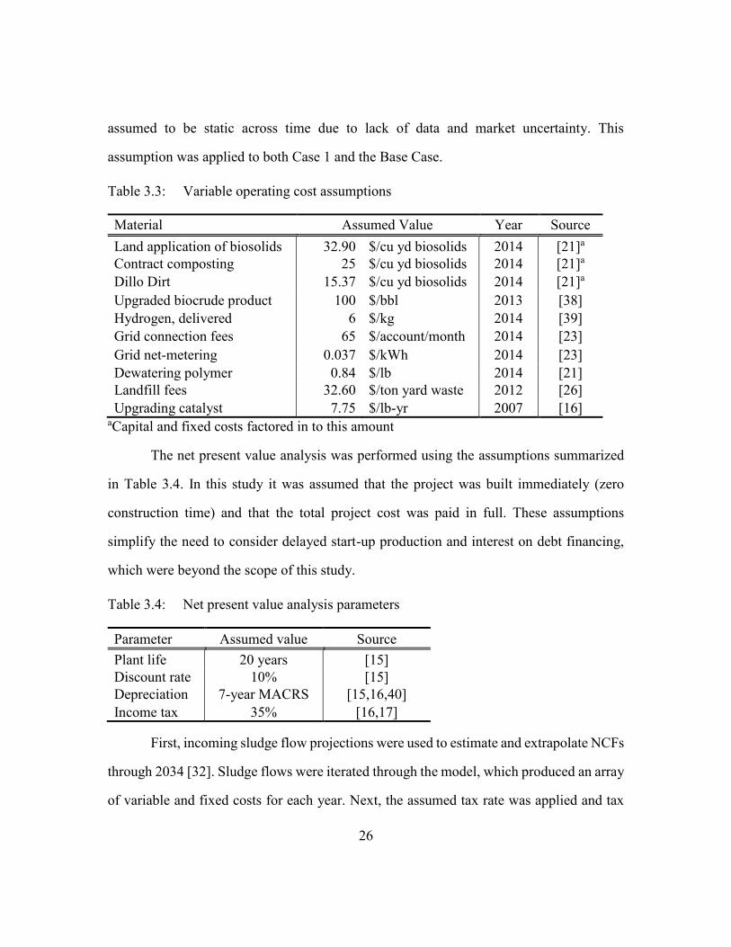
Table 3.3 reports variable operating costs which include all inputs and outputs
required for daily plant operation. These costs can be highly variable depending on current
market prices, especially in the case of crude oil price [38]. Thus variable costs were
26
assumed to be static across time due to lack of data and market uncertainty. This
assumption was applied to both Case 1 and the Base Case.
Table 3.3: Variable operating cost assumptions
Material Assumed Value Year Source
Land application of biosolids 32.90 $/cu yd biosolids 2014 [21]a
Contract composting 25 $/cu yd biosolids 2014 [21]a
Dillo Dirt 15.37 $/cu yd biosolids 2014 [21]a
Upgraded biocrude product 100 $/bbl 2013 [38]
Hydrogen, delivered 6 $/kg 2014 [39]
Grid connection fees 65 $/account/month 2014 [23]
Grid net-metering 0.037 $/kWh 2014 [23]
Dewatering polymer 0.84 $/lb 2014 [21]
Landfill fees 32.60 $/ton yard waste 2012 [26]
Upgrading catalyst 7.75 $/lb-yr 2007 [16] aCapital and fixed costs factored in to this amount
The net present value analysis was performed using the assumptions summarized
in Table 3.4. In this study it was assumed that the project was built immediately (zero
construction time) and that the total project cost was paid in full. These assumptions
simplify the need to consider delayed start-up production and interest on debt financing,
which were beyond the scope of this study.
Table 3.4: Net present value analysis parameters
Parameter Assumed value Source
Plant life 20 years [15]
Discount rate 10% [15]
Depreciation 7-year MACRS [15,16,40]
Income tax 35% [16,17]
First, incoming sludge flow projections were used to estimate and extrapolate NCFs
through 2034 [32]. Sludge flows were iterated through the model, which produced an array
of variable and fixed costs for each year. Next, the assumed tax rate was applied and tax

27
credits from depreciation were added in. Finally the discount rate was applied to each year
and all years were summed. The NPV of Case 1 was then calculated by subtracting the
initial investment cost, which is summarized by,
𝑁𝑃𝑉𝐶𝑎𝑠𝑒 1 = ∑ [𝑁𝐶𝐹 ∗ (1 − 𝑡) + 𝑡𝐷𝑖𝐶0
(1 + 𝑑)𝑖] − 𝐶0
𝑓𝑖𝑛𝑎𝑙 𝑦𝑒𝑎𝑟
𝑖=1
(6)
where 𝑑 is the discount rate, 𝑡 is the federal tax rate, 𝐷 is the depreciation rate, 𝐶0 is the
total capital investment and 𝑖 is number of years after the project year.
Discount rate can be thought of as the inverse of compound interest as it represents
the present value of future money. The discount rate chosen for this study was somewhat
high to account for variation and uncertainty in the variable and fixed costs. Aden et al.
also justifies this discount rate as being appropriate for renewable energy investments as
determined in a previous study [15].
In order to obtain overall savings, the Base Case was integrated into Equation (6)
using the same assumptions and methods as Case 1. Depreciation and capital costs for the
Base Case were assumed to be built into the variable costs as reported in Table3.3. Taxes
were not taken into account due to the negative yearly NCF. In comparing Case 1 to the
Base Case we get the overall NPV,
𝑁𝑃𝑉 = ∑ [(𝑁𝐶𝐹 ∗ (1 − 𝑡) + 𝑡𝐷𝑖𝐶0)𝐶𝑎𝑠𝑒 1,𝑖 − (𝑁𝐶𝐹)𝐵𝑎𝑠𝑒 𝐶𝑎𝑠𝑒,𝑖
(1 + 𝑑)𝑖 ] − 𝐶0
𝑓𝑖𝑛𝑎𝑙 𝑦𝑒𝑎𝑟
𝑖=1
(7)
ROI was calculated as,
28
𝑅𝑂𝐼 =𝑁𝑃𝑉
𝑇𝐶𝐼 (8)
Pay-back time was calculated by finding the year in which the NPV became
positive. Linear interpolation was then used to estimate the pay-back day in that year in
order to report a higher resolution result.
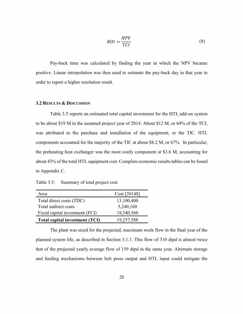
3.2 RESULTS & DISCUSSION
Table 3.5 reports an estimated total capital investment for the HTL add-on system
to be about $19 M in the assumed project year of 2014. About $12 M, or 64% of the TCI,
was attributed to the purchase and installation of the equipment, or the TIC. HTL
components accounted for the majority of the TIC at about $8.2 M, or 67%. In particular,
the preheating heat exchanger was the most costly component at $3.6 M, accounting for
about 43% of the total HTL equipment cost. Complete economic results tables can be found
in Appendix C.
Table 3.5: Summary of total project cost
Area Cost [2014$]
Total direct costs (TDC) 13,100,400
Total indirect costs 5,240,160
Fixed capital investment (FCI) 18,340,560
Total capital investment (TCI) 19,257,588
The plant was sized for the projected, maximum week flow in the final year of the
planned system life, as described in Section 3.1.1. This flow of 310 dtpd is almost twice
that of the projected yearly average flow of 159 dtpd in the same year. Alternate storage
and feeding mechanisms between belt press output and HTL input could mitigate the

29
effects of these rare peak flows. These alternate strategies could significantly lower the
total project cost by reducing system size.
Despite its high design capacity, the HTL and upgrading system considered in this
study was much smaller than systems considered in the corresponding literature.
Component size ratios varied from 1-45% with a median size ratio of 1.4%, which shows
that most components were scaled down significantly. It is not explicitly stated in the
literature at what limit the scaled equipment cost assumption begins to break down.
However, we expect that at this low extreme there exists significant uncertainty in the
results. Overall, this indicates that further study should consider requesting new quotes for
components at this smaller scale.
Table 3.6 reports the economic results of Case 1 over the 20 year project life. Return
on investment of the project was calculated to be about 1.7 with a pay-back time of about
4.4 years. Savings for the CoA was estimated to be on the order of $32 M. These values
are considered to be very conservative based on the scaling uncertainty described earlier in
this section. Uncertainty with regard to installation and cost of an untested technology on
this scale further contribute to potential over-estimation of the project cost.
Table 3.6: Case 1 lifetime economics
Parameter Value
NPV [2014$] 32,165,447
Pay-back time [yr] 4.35
ROI 1.67
Figure 3.2 shows a graphical representation of how the NPV of the project changes
across its lifetime. Pay-back time is clearly shown where the curve crosses the x-axis. The
highest rate of economic gain is represented by the steepest positive slope of the curve.
This occurs at the beginning of the project life when the depreciation is minimizing the

30
federal tax burden. The curve levels off towards the end of the project due to the increasing
uncertainty in the present value of future money in those years. However, the curve does
not completely level off, which suggests that there could be additional profit made from
extending the life of the project.
Figure 3.2: Variation of NPV across the life of the project
The 20 year plant life assumption is conservative. Literature values for plant life
ranged from 20-30 years [15–17]. Originally the study was planned to match the HTL plant
life to that of HBBMP, however HBBMP does not have a set lifetime. Instead processes
and equipment are occasionally updated and retrofitted as components break down, show
signs of wear or technologies are updated. Thus, while these initial calculations were based
on a 20 year life, it is expected that the actual life of the plant would be much longer. This
becomes especially true as the technology matures and more full-scale HTL plants are
installed. These insights will only cause ROI to increase.
-20
-10
0
10
20
30
40
2014 2019 2024 2029 2034NP
V [
Mill
ion
20
14
$]
Project Life [year]

31
Finally, in this initial study of a proposed HTL plant it was necessary to consider
on-site upgrading in order to assign an accurate price to the final upgraded biocrude
product. In practice existing petroleum refineries already contain the needed infrastructure
to perform upgrading at a favorable economy of scale. Leveraging this infrastructure would
decrease the capital, fixed and variable costs of the HTL system proposed here. Future
studies should consider collaboration with a petroleum refining company to explore the
costs involved with blending or processing biocrude on a significantly large scale.
3.3 SENSITIVITY
Figure 3.3 reports that ROI was most sensitive to the total installed cost (TIC). This
directly concerns the system sizing as discussed in Section 3.2. The TIC value of $21.3 M
is calculated from the sizing assumption of maximum day flow in 2034. This is the largest
flow that the HTL and upgrading system could be reasonably sized for and results in an
ROI of 0.65. Alternatively, the TIC could be as low as $7.7 M if the system were sized for
the average yearly flow in 2034. This results in an ROI of 3.07, but would cause the system
to possibly become overloaded in its final year or even earlier. An alternative storage and
feeding system to mitigate peak flows, as discussed in Section 3.2, could reduce uncertainty
in component scaling and significantly increase ROI.

32
Figure 3.3: Sensitivity of chosen parameters with regards to ROI
The discount rate has the greatest potential to increase ROI based on the change of
a single parameter. The value of 10% used in this study took into account the uncertainties
related to establishing a new technology. Previous TE studies had used this value with
respect to renewable energy projects in general. This analysis showed that decreasing the
discount rate to a value closer to that of typical depreciation in the US would significantly
increase the ROI to about 3.6. As the technology becomes mature, and more plants are
constructed, this shift is expected to happen naturally.
Biocrude price is the third most sensitive parameter with regards to ROI. It has the
potential to lower ROI significantly, but is expected to be in an almost constant state of
fluctuation as it follows the current market value. At a price of $40/bbl the resulting ROI
21.31
10
40
9.4
0
60
25
14.5
28
300
7.73
3
120
40
100
30
443
4
42
270
0.00 0.50 1.00 1.50 2.00 2.50 3.00 3.50 4.00 4.50
TIC [M$]
Discount rate [%]
Biocrude price [$/bbl]
Biocrude yield [% afdw]
Yard waste to HTL [%]
Indirect costs [%]
Preheater heat transfer coefficient[BTU/hr/ft2/°F]
Other direct costs [%]
Tax rate [%]
Temp out of HX [°C]
ROI
33
is 0.96. Oil prices have been generally increasing since the late 1990s, with some major
increases and decreases leading to the present [41]. Thus, it is expected that over the 20
year life of the project that oil prices should not have a large negative effect on ROI.
Additionally, future federal policy could help in this regard if biocrude were to be
considered a renewable fuel, and thus be eligible for federal incentives that could protect
HTL projects from large fluctuations in crude oil pricing.
Yard waste to HTL is an idea that is discussed thoroughly in Section 6.2. In this
analysis the values range from 0% of yard waste included in the HTL stream, which is the
value used in Case 1, to 100% of yard waste to HTL. At 100% yard waste to HTL, all
landfilling costs are mitigated and biocrude production increases from the additional
biomass. Added costs associated with additional required infrastructure were not
considered, but are expected to be minimal in comparison with the economic gain.
A two-factor sensitivity analysis was also performed with regards to ROI. This
analysis allowed for a better realization of potential gains in ROI. Parameter combinations
were sorted according to greatest ROI impacts. The top six combinations are reported in
Figure 3.4.

34
Figure 3.4: Two-factor sensitivity analysis results for ROI. The top six combinations are
reported in order of greatest increase in ROI.
This two-factor analysis shows that combining a smaller system size with a less
uncertain discount factor could produce an ROI of around 6. Combinations that include
yard waste to HTL are expected to have a slightly lower ROI than reported due to a possible
minor increase in capital cost. Overall these six different combinations show an ROI
around or in excess of 4. This is especially reasonable since parameters like TIC and
discount rate should decrease as the technology is implemented across increasing numbers
of projects. Alternatively, if the TIC hits its maximum at the same time that biocrude price
or biocrude yield hit their minimum, the ROI can drop as low as 0.24 or 0.28 respectively.
21.31 & 10
10 & 0
21.31 & 0
9.4 & 10
10 & 60
40 & 10
7.73 & 3
3 & 100
7.73 & 100
40 & 3
3 & 30
120 & 3
-2.00 -1.00 0.00 1.00 2.00 3.00 4.00 5.00 6.00 7.00 8.00 9.00
TIC [M$] & Discount rate [%]
Discount rate [%] & Yard waste to HTL [%]
TIC [M$] & Yard waste to HTL [%]
Biocrude yield [% afdw] & Discount rate [%]
Discount rate [%] & Indirect costs [%]
Biocrude price [$/bbl] & Discount rate [%]
ROI

35
3.4 CONCLUSION
This chapter showed that economic impacts of a sludge HTL project have the
potential to be favorable. It was shown that in the case of local implementation at HBBMP
that this project could save the CoA on the order of $32 M. This estimate is thought to be
conservative by the authors, which is further suggested by the sensitivity analysis. The two-
factor sensitivity analysis reported a maximum ROI of around 6 when considering the
simultaneous, best case scenario for TIC and discount rate. Both of these parameters are
expected to move towards their best case scenario as more plants are built and the
technology matures, thus greatly increasing ROI.
36
Chapter 4
Greenhouse Gas Emissions
4.1 ANALYSIS
This study analyzed the impacts on GHG emissions, as a result of implementing
Case 1, in the following three ways: 1) Case 1 sludge-to-gasoline production versus
standard petroleum-to-gasoline (P2G) production, 2) sludge mitigation via Case 1 versus
the Base Case and 3) Case 1 sludge-to-gasoline versus the total business-as-usual (BAU)
scenario. Table 4.1, at the end of this section, presents a summary of the operational
parameters used for these analyses.
Figure 4.1 presents a graphical representation of the BAU scenario. The boundaries
between biosolids production and petroleum fuel production do not overlap, thus the
emissions produced by both sectors are additive. GHG baseline factors were modeled in
MS Excel 2013 using literature data and tools available online, including the GREET
(Greenhouse Gases, Regulated Emissions, and Energy Use in Transportation) and NETL
(National Energy Technology Laboratory) models [42,43].

37
CO2e
Energy Petroleum-to-gasoline (P2G)
Base CaseFood Cycle/Consumption/Wastewater Treatment
Digestion
Biogas
Solids
Composting and Land
Application
Cogen & Boilers
Flare
Sludge
CO2
CO2e
Drilling & Recovery
RefiningPump/
CombustionTransport
Transport/Blending
Figure 4.1: GHG emissions boundaries with respect to business-as-usual. Biosolids and
petroleum fuel production do not affect one another, but both generate GHGs.
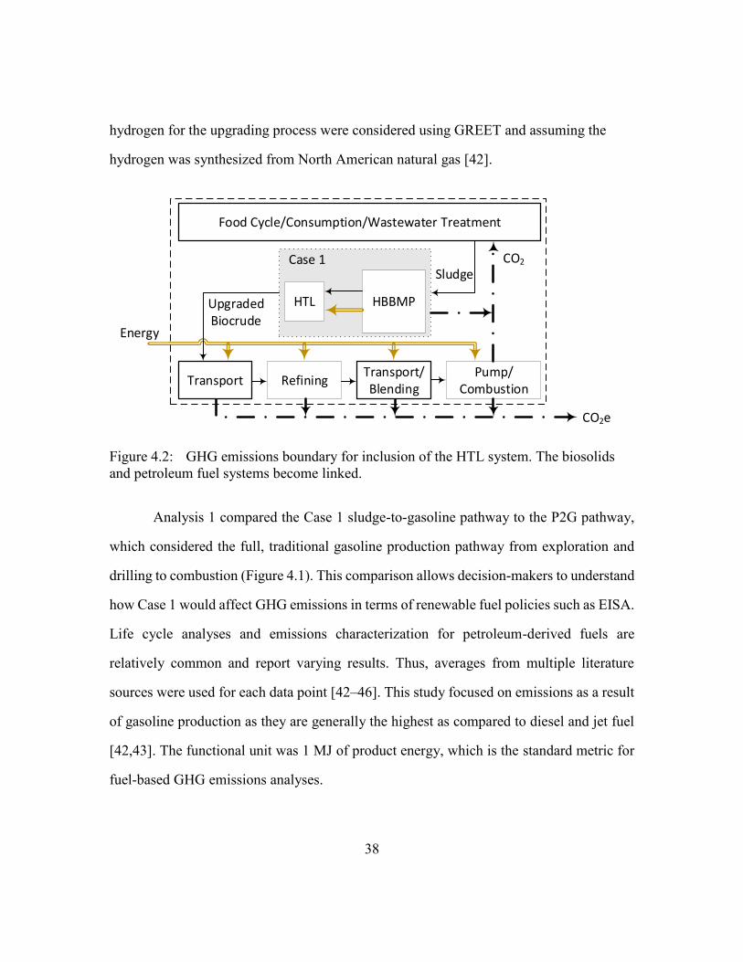
Figure 4.2 shows how Case 1 caused the BAU systems from Figure 4.1 to couple.
Biocrude production and HTL processing effectively replace both petroleum exploration
and extraction, as well as composting and land application of biosolids, but add emissions
due to hydrogen use and previously-deferred fertilizer production. Emissions from
fertilizer production were calculated assuming that fields using biosolids as a source of
nitrogen would require the same amount of nitrogen from an alternate source. These
emissions were calculated using GREET and assumed that the nitrogen fertilizer was
synthesized from ammonia [42]. Emissions related to the production of additional
38
hydrogen for the upgrading process were considered using GREET and assuming the
hydrogen was synthesized from North American natural gas [42].
HBBMP
RefiningPump/
Combustion
HTL
Sludge
CO2e
Transport/Blending
Energy
Transport
Food Cycle/Consumption/Wastewater Treatment
Upgraded Biocrude
Case 1 CO2
Figure 4.2: GHG emissions boundary for inclusion of the HTL system. The biosolids
and petroleum fuel systems become linked.
Analysis 1 compared the Case 1 sludge-to-gasoline pathway to the P2G pathway,
which considered the full, traditional gasoline production pathway from exploration and
drilling to combustion (Figure 4.1). This comparison allows decision-makers to understand
how Case 1 would affect GHG emissions in terms of renewable fuel policies such as EISA.
Life cycle analyses and emissions characterization for petroleum-derived fuels are
relatively common and report varying results. Thus, averages from multiple literature
sources were used for each data point [42–46]. This study focused on emissions as a result
of gasoline production as they are generally the highest as compared to diesel and jet fuel
[42,43]. The functional unit was 1 MJ of product energy, which is the standard metric for
fuel-based GHG emissions analyses.

39
Analysis 2 compared Case 1 to the Base Case in terms of GHG emissions produced
in the process of converting sludge to a safe, useful product. For the Base Case this was
the production of biosolids and compost, and for Case 1 this was the production of biocrude
oil. The system boundary in Analysis 2 ends at the point where the upgraded biocrude oil
is transported off-site. The functional unit used for Analysis 2 was 1 dry kg of incoming
sludge. This was due to the two cases having an identical input. This analysis is important
because it shows how Case 1 affects GHG emissions locally.
Finally, Analysis 3 compared the Case 1 sludge-to-gasoline scenario to the BAU
scenario. The comparison was made on a total CO2-equivalent (CO2e) per year basis in
order to see overall impact. This analysis was important because implementation of Case
1 affects both the biosolids manufacturing and petroleum industries simultaneously.
In the Base Case energy requirements are fulfilled on-site from biogas capture and
utilization. Excess biogas is flared in order to mitigate methane (CH4) emissions, which
are about 25 times more environmentally impactful than CO2 over a 100 year period [43].
Carbon emissions from the combustion of biogas were excluded from calculations in
accordance with international convention set forth by the Intergovernmental Panel on
Climate Change (IPCC) [47]. This convention states that the carbon released from the
combustion of biomass and its products is assumed to be balanced with the carbon uptake
from the biomass while it was growing. In this analysis the sludge that enters HBBMP was
assumed to be composed entirely of biomass produced from the food cycle. This exclusion
is limited to CO2 only, as other GHGs such as CH4 and nitrous oxide (N2O) will not be
reabsorbed into the cycle.
The City of Austin (CoA) reported that biogas combustion was considered a
carbon-neutral alternative source to grid electricity and natural gas use. In addition to the
zero emissions from biogas combustion, additional credits were applied for offsetting grid

40
and natural gas energy [32]. It is the opinion of the authors that the additional credits are
considered double counting. In this study credit was given only to electricity generated
from biogas combustion that was supplied to the grid in excess of what was used on-site.
If excess biogas was contributed to natural gas infrastructure a credit would be appropriate
there as well, but currently this is not the case.
Operational emissions at HBBMP come from the use of diesel fuel on-site and the
off-site production of chemicals required for composting and dewatering. Diesel fuel is
used in vehicles that manage composting, transport biosolids for land application and apply
biosolids to the grass fields on-site. Embedded energy and emissions of the existing
infrastructure were not considered.
Table 4.1: Model parameters and assumptions used in GHG analysis
Parameter Assumed Value Source
Conventional gasoline LHV 44 MJ/kg [43] Conventional gasoline density 2.8 kg/gal [43] Diesel LHV 42 MJ/kg [42] Diesel GHG 76.7 kg CO2e/mmBTU [43] Nitrogen fertilizer production 3.3 kg CO2e/kg N [42] Hydrogen production (from natural gas) 18.4 kg CO2e/kg H2 [42] Emissions from electricity (ERCOT mix) 616 g/kWh [42] Industrial natural gas emissions 54.7 kg CO2e/mmBTU [48] Nitrogen content in biosolids cake 3.9 % [29] Distance to refinery 150 mi Crude tanker truck capacity 210 bbl/load Crude tanker truck fuel economy 6.5 mi/gal
4.2 RESULTS & DISCUSSION
Figure 4.3 reports that GHG emissions were reduced in the P2G scenario by about
30 gCO2e/MJ, or 33%. The majority of emissions from standard gasoline production occur

41
at the tailpipe. Nearly all of those emissions were removed in Case 1 due to the organic
nature of the feedstock. Only non-CO2 GHG emissions were counted, which were almost
negligible at less than 1 gCO2e/MJ. Emissions due to production increased by about 16
gCO2e/MJ from the P2G scenario to Case 1. This was due to consideration of on-site
hydrogen use in the upgrading system. Typically these emissions would occur at the
refinery, and thus be counted in the refinery emissions profile. Since Case 1 considered
both on-site upgrading and refinement in a traditional refinery, it could be possible that the
hydrogen use was being double-counted. Higher resolution data of refinery emissions
would help to solve this and could further reduce the Case 1 GHG emissions.

42
Figure 4.3: Comparison of GHG emissions per MJ of energy for gasoline production via
standard P2G and Case 1
Emission reduction in Case 1 came from credit given for excess electricity
contributed to the grid, as explained in Section 4.1. This power contribution directly offset
emissions that would have been generated according to the standard ERCOT fuel mix.
Figure 4.4 reports that GHG emissions were increased in the sludge mitigation
scenario by about 45 gCO2e/kg sludge, or 187%. The majority of GHG emissions from
Case 1, 71.6 gCO2e/kg sludge, were attributed to external nitrogen fertilizer production,
which is typically deferred by land application of biosolids and composting. This is
assuming that the fields typically utilizing biosolids for nitrogen would need to completely
replace that nitrogen with an alternate source, as explained in Section 4.1. Alternatively, in
91.6
61.0
-40.00
-20.00
0.00
20.00
40.00
60.00
80.00
100.00
P2G Case 1
GH
G E
mis
sio
ns
[g C
O2e/
MJ]
Nitrogen fertilizerproduction
Excess electricity togrid
Production
Combustion
Net total

43
the absence of available biosolids, less nitrogen could be applied to the fields. It may also
be acceptable for the fields to produce less. If either of these cases are true then emissions
would be greatly reduced. Additionally, hydrogen use was a large contributor with almost
34 gCO2e/kg sludge.
Figure 4.4: Comparison of GHG emissions per kg of incoming sludge between the Base
Case and Case 1
The majority of GHG emissions generated in the Base Case, about 59 gCO2e/kg
sludge, came from on-site diesel fuel usage. Diesel is mostly used for the composting
operations and to transport biosolids for land application. The rest is attributed to the
production of chemicals used in the biosolids and composting processes. Figure 4.4 shows
24.0
68.7
-60.00
-40.00
-20.00
0.00
20.00
40.00
60.00
80.00
100.00
120.00
Base Case Case 1
GH
G E
mis
sio
ns
[g C
O2e/
kg s
lud
ge]
Hydrogenproduction
Nitrogen fertilizerproduction
Excess electricity togrid
Chemical production
Diesel use
Net total

44
that the diesel and chemical use in the Base Case were almost completely mitigated in Case
1 due to removal of the composting operation.
Figure 4.5 shows that overall, Case 1 reduced GHG emissions by about 44% as
compared to the uncoupled BAU scenario. For the P2G scenario, the model predicted a
savings of about 1500 MT CO2e/y over traditional gasoline production. With respect to the
impacts at HBBMP, the model reported an increase of about 1460 MT CO2e/y. The overall
savings comes from the BAU case being additive, while additional Case 1 emissions
incurred from conversion of biocrude to gasoline are small.
Figure 4.5: Total GHG emissions per year for BAU vs. Case 1. Despite an increase in
sludge treatment emissions at HBBMP, overall GHG emissions are reduced by about
40%.
5325
3024
0
1000
2000
3000
4000
5000
6000
BAU Case 1
[MT
CO
2e/
y]
Sludge treatment
Gasoline production &use
Total

45
4.3 SENSITIVITY
Figure 4.6 reports the sensitivity of emissions parameters with respect to the P2G
scenario. This figure indicates which parameters are capable of altering the sludge HTL-
derived gasoline qualifications under RFS2 standards. To be considered a renewable fuel
there must be a 20% reduction in GHG emissions over the standard P2G baseline. A 50%
reduction qualifies the fuel as an advanced biofuel.
Figure 4.6: Sensitivity of selected parameters with regards to reduction in GHG
emissions of Case 1 compared to the P2G scenario. EISA RFS2 category limits are
shown by the gray dashed lines.
No
0.13
100
50
500
Yes
0.038
0
100
20
-40% -20% 0% 20% 40% 60% 80% 100% 120% 140% 160%
Second co-gen
H2 Feed rate [kg/kg biocrude]
Hydrogen double-count [%]
Cake diverted to HTL [%]
Distance to refinery [mi]
GHG emissions reduction vs P2G scenario
Bas
elin
e
Ren
ewab
le F
uel
Ad
van
ced
Bio
fuel

46
The greatest reductions to GHG emissions are gained through the “What-If”
scenarios proposed in this analysis. The first of which was the addition of a second co-gen
unit, which results in a 134% reduction. A reduction of this magnitude would result in Case
1 producing negative net emissions. This would be achieved by offsetting more GHGs from
the ERCOT power mix than are produced from making and combusting the fuel. This
scenario would affect ROI in a negative way, but could be very beneficial if ROI is already
high. A similar scenario would involve contributing excess biogas to a gas distribution line.
Hydrogen double-counting was considered as a possibility in Section 4.1. In this
analysis the effect of mitigating this possibility is reported. Figure 4.6 shows that in the
case of complete hydrogen double-counting there would be a 60% reduction in GHG
emissions. This alone would qualify the sludge HTL-derived gasoline as an advanced
biofuel which may cause additional government funding to become available. It is most
likely that only some percentage of the hydrogen was double-counted in Case 1, so it is
expected that overall GHG emissions reduction would be between the reported 33% and
the possible 60% seen in Figure 4.6.
4.4 CONCLUSION
This chapter showed that eligibility of sludge HTL-derived gasoline as a renewable
fuel is attainable and likely. Two major assumptions in these analyses caused a significant
amount of uncertainty in the results. The first was the assumption that fields currently using
biosolids fertilizer required a fixed amount of nitrogen. This meant that all biosolids
diverted from land application to HTL would cause an increase in external nitrogen
fertilizer production, which greatly increased overall emissions. The second assumption
was that hydrogen use for biocrude upgrading was not included in the refinery data, thus

47
needing to be included with the on-site calculations. The impacts of this assumption were
further investigated using sensitivity analysis in Section 4.3.
Overall, GHG emissions would be reduced by implementation of the sludge HTL
technology, but the magnitude of this impact is uncertain. If farms were able to reduce their
nitrogen requirements or additional steps were taken to recover nitrogen from other HTL
products, GHG emissions could be further reduced. Furthermore, GHG emissions could be
reduced if biocrude upgrading were performed at the refinery instead of on-site. Finally, a
major barrier is the amount of mass produced. At this magnitude of fuel production, total
emission reduction is minimal.
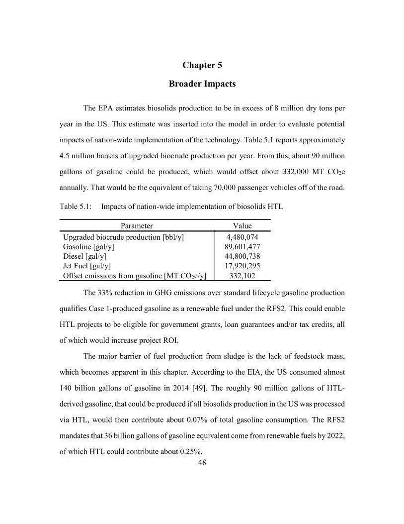
48
Chapter 5
Broader Impacts
The EPA estimates biosolids production to be in excess of 8 million dry tons per
year in the US. This estimate was inserted into the model in order to evaluate potential
impacts of nation-wide implementation of the technology. Table 5.1 reports approximately
4.5 million barrels of upgraded biocrude production per year. From this, about 90 million
gallons of gasoline could be produced, which would offset about 332,000 MT CO2e
annually. That would be the equivalent of taking 70,000 passenger vehicles off of the road.
Table 5.1: Impacts of nation-wide implementation of biosolids HTL
Parameter Value
Upgraded biocrude production [bbl/y] 4,480,074
Gasoline [gal/y] 89,601,477
Diesel [gal/y] 44,800,738
Jet Fuel [gal/y] 17,920,295
Offset emissions from gasoline [MT CO2e/y] 332,102
The 33% reduction in GHG emissions over standard lifecycle gasoline production
qualifies Case 1-produced gasoline as a renewable fuel under the RFS2. This could enable
HTL projects to be eligible for government grants, loan guarantees and/or tax credits, all
of which would increase project ROI.
The major barrier of fuel production from sludge is the lack of feedstock mass,
which becomes apparent in this chapter. According to the EIA, the US consumed almost
140 billion gallons of gasoline in 2014 [49]. The roughly 90 million gallons of HTL-
derived gasoline, that could be produced if all biosolids production in the US was processed
via HTL, would then contribute about 0.07% of total gasoline consumption. The RFS2
mandates that 36 billion gallons of gasoline equivalent come from renewable fuels by 2022,
of which HTL could contribute about 0.25%.

49
In order to make a significant impact on fuel production, alternative feedstocks
should be considered. Farm animal manure is produced in the US at an estimated rate of
about 250 million dry tons per year and is considered in several HTL studies [3–5,50]. Our
model predicts that a feedstock of this magnitude could result in about 2.8 billion gallons
of gasoline per year, or 8% of the total RFS2 mandate in 2022, and a reduction of 10.5
million MT CO2e or the equivalent of 2.2 million passenger vehicles.
50
Chapter 6
Conclusion & Recommendations
6.1 SUMMARY
HTL is a novel and versatile mitigation option for sludge and biosolids, and could
be very attractive economically. The conservative estimate calculated in this study showed
savings of about $32 million over the 20 year life of the project. This is significant for a
semi-mandatory facility that typically operates at an economic loss.
Contributions as a renewable fuel source are minimal due to limited feedstock.
GHG emissions were reduced, but impact at this scale was relatively low. However,
sensitivity analysis showed that adding an additional co-gen unit could cause the process
to produce fuel at net negative emissions. Consideration of farm animal manure as a
feedstock for a biosolids HTL plant could 1) significantly increase national impact as a fuel
source and 2) offset a significant amount of GHG emissions.
6.2 RECOMMENDATIONS FOR FUTURE RESEARCH
There are numerous engineering details that should be addressed in future studies
in order to generate more accurate TE analyses for sludge HTL. In terms of project
economics, future studies should consider the following: 1) Obtain quotes from vendors on
components that are closer to the required size will minimize scaling uncertainties as
discussed in Section 3.2. 2) Investigate methods for transferring or storing the biosolids
from the end of the biosolids process to the HTL system that would accommodate extreme
flow rate fluctuations. 3) Consider process downtime. TE analyses from the literature tend
to assume a certain amount of “stream days” per year to account for downtime [16,17].
However, HBBMP has recursive parallel systems so that if a component breaks down, the

51
flow can shift to a parallel track and continue to run continuously. This same parallel
process design should be investigated and optimized for the HTL system so that the process
would operate continuously along with HBBMP.
In this study the HTL process was optimized for daily production value, which
ultimately corresponded to maximizing fuel production. Future studies may want to
optimize operations in other ways such as minimizing GHG emissions, pay-back time or
maximizing ROI or EROI. The framework generated and the dynamic model implemented
in this study accommodates for these future studies to be conducted.
Optimization of the HTL feedstock could also be considered. Pre-digested sludge
has a higher VS content than that of biosolids cake, which would result in an increased
biocrude yield. A separate case could then be modeled that extracts both pre-digested
sludge, which would decrease biogas production, and biosolids cake, so that the biogas
stream was fully utilized. The optimization could be based on attaining maximum EROI,
economic value or biogas usage.
It was assumed that as biosolids were diverted from composting to HTL, city yard
waste typically mixed with those biosolids was then diverted to the local landfill at a
specified cost. In this study this cost was the largest daily cost in Case 1. This cost could
be mitigating by further research in two areas: 1) multi-component HTL feedstock streams
and 2) 3rd-party composting.
1) The organic nature of the yard waste should allow it to be added to the HTL input
stream and processed into biocrude. Research should be done on how multi-
component feedstock streams affect HTL yields and biocrude compositions and
what additional equipment would be needed. Fats, oils and grease are also collected
by the CoA, but are typically dewatered and landfilled or disposed of at hazardous
52
waste facilities [27]. These materials have very high VS content which could
increase biocrude yields significantly if added to the HTL feedstock stream.
Overall, multi-component feedstock streams could improve sludge HTL by 1)
increasing total feedstock mass potential, 2) increasing oil yields and EROI, 3)
decreasing alternative disposal costs and 4) decreasing GHG emissions related to
alternative disposal methods.
2) Excess yard waste diverted to a 3rd-party composting service would still incur some
cost, although possibly less than that of a landfill. It would also continue to create
a benefit environmentally. Additionally, it may be appropriate to credit back some
GHG emissions from external fertilizer production as some mass percentage of the
compost would contain nitrogen.
Our results show that in both cases there is a large amount of excess biogas that
could be used to fuel additional heat-intensive processes at the HMMBP complex.
Processes considered in other works include on-site hydrogen production and catalytic
hydrothermal gasification (CHG). CHG can be used to recover CH4 and significant
amounts of nitrogen from the HTL and upgrading aqueous byproducts [4,16,28]. This
nitrogen source could be used to replace fertilizer requirements typically fulfilled by land
application of biosolids and composting, which would drastically reduce GHG emissions
associated with Case 1. However, capital cost would increase significantly. Further testing
of the aqueous HTL byproducts should be performed to estimate possible impacts versus
cost.

53
Appendices
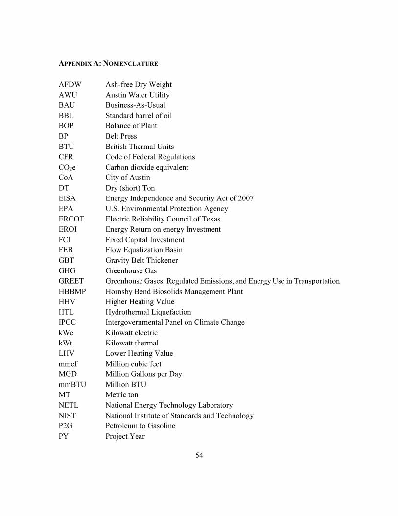
54
APPENDIX A: NOMENCLATURE
AFDW Ash-free Dry Weight
AWU Austin Water Utility
BAU Business-As-Usual
BBL Standard barrel of oil
BOP Balance of Plant
BP Belt Press
BTU British Thermal Units
CFR Code of Federal Regulations
CO2e Carbon dioxide equivalent
CoA City of Austin
DT Dry (short) Ton
EISA Energy Independence and Security Act of 2007
EPA U.S. Environmental Protection Agency
ERCOT Electric Reliability Council of Texas
EROI Energy Return on energy Investment
FCI Fixed Capital Investment
FEB Flow Equalization Basin
GBT Gravity Belt Thickener
GHG Greenhouse Gas
GREET Greenhouse Gases, Regulated Emissions, and Energy Use in Transportation
HBBMP Hornsby Bend Biosolids Management Plant
HHV Higher Heating Value
HTL Hydrothermal Liquefaction
IPCC Intergovernmental Panel on Climate Change
kWe Kilowatt electric
kWt Kilowatt thermal
LHV Lower Heating Value
mmcf Million cubic feet
MGD Million Gallons per Day
mmBTU Million BTU
MT Metric ton
NETL National Energy Technology Laboratory
NIST National Institute of Standards and Technology
P2G Petroleum to Gasoline
PY Project Year

55
ROI Return on Investment
TDC Total Direct Cost
TE Techno-economic
TIC Total Installed Cost
Ton Short ton
VS Volatile Solids
WWTP Wastewater Treatment Plant

56
APPENDIX B: ADDITIONAL MASS & ENERGY MODEL RESULTS
Stream designators in each table included in this appendix correspond to the Case
1 process diagram located in Chapter 2 (Figure 2.2). All mass results include water
content.
Table B1: Case 1 mass flow results with TS, VS and HTL temperature and pressure
data.
Stream Description Mass
[MT/d] TS [%] VS [% afdw]
2 FEB out 5776 1.6 71.7
3 GBT In 5776 1.5 72.4
4 Digester In 1057 7.2 67.7
5 Digester Out 1035 5.4 46.4
6 BP In 1035 5.4 46.4
7 BP Out 253 19.8 54.4
8 Land App 0 - -
9 Compost In 0 - -
10 To Dillo Dirt 0 - -
11 To Contract 0 - -
Temperature Pressure
[°C] [°F] [MPa] [psi]
12
Dewatered
biosolids to HTL 253 21 70 0.1 14.7
13
High pressure to
heat exchanger 253 22.6 73 21.0 3050
14 To HTL reactor 253 280 536 20.7 3000
15
HTL to heat
exchanger 253 350 662 20.7 3000
16
HTL products out
of HX to filter 253 74.6 166 20.3 2950
17 Filter out (Char) 2.72 21 70 0.1 14.7
18
HTL products -
char 250 74.6 166 20.0 2900
19 Biocrude 8.16 74.6 166 10.5 1530
- Upgrade preheat 8.16 171 339 10.5 1530
- Hydrotreater 8.16 400 752 10.5 1530
20 Upgraded biocrude 6.85 21 70 0.1 14.7

57
Table B2: Case 1 heat and energy flow results
Stream Description
Heat
[GJ/d]
Power
[kWh/d]
H1 Co-gen heating 97 -
H2 Additional AD heating 10 -
H3 HTL heating 106 -
H4 Upgrade heating 7 -
E1 Co-gen power - 20352
- Base Case power - 12842
E6 Grid net-metering - 5535
E7 HTL pumping - 1859
E8 Upgrade pumping - 116
Table B3: Case 1 gas flow results.
Stream Description Mass
[MT/d]
Volume
[m3/d] [mmcf/d]
G1 Biogas produced 22.3 25252 0.89
G2 To Cogen 8.1 9179 0.32
G3 To Boilers 5.1 5717 0.20
G4 Flare-off 9.2 10357 0.37
G5 HTL off gas 3.5 - -
G6 Hydrogen for upgrading 0.16 - -
G7 H2 recycle 0.24 - -
G8 Upgrading off-gas 0.25 - -
G9 Total off-gas 3.8 - -

58
Table B4: Water and other mass flow results
Stream Description
Mass
[MT/d] TS [%]
W1 GBT Wash 6370 0.21
W2 BP Wash 1764 0.32
W3 Secondary In 8133 0.23
W4 To Ponds 8218 0.00
W5 HTL aqueous phase 239 0.00
W6 Upgrading aqueous phase 1.25 0.00
W7 Total aqueous phase 240 0.00
P1 Polymer prior to GBT 0.27 -
P2 Polymer prior to BP 0.47 -
YW Yard Waste input from city 75 -

59
APPENDIX C: ADDITIONAL ECONOMIC MODEL RESULTS
Table C1: Results for TCI based on TIC and Table 3.2
[2014$]
Total installed cost (TIC) 12,243,365
Other direct costs
Buildings 122,434
Site Development 122,434
Add. Piping 612,168
Total direct costs (TDC) 13,100,400
Indirect costs
Prorated expenses 1,310,040
Construction fee 655,020
Field expenses 1,310,040
Project contingency 1,310,040
Startup & permits 655,020
Total indirect costs 5,240,160
Fixed capital investment (FCI) 18,340,560
Working capital 917,028
Total capital investment (TCI) 19,257,588

60
Table C2: Variable operating cost results based on 2014 mass flow and calculated
using assumptions in Table 3.3
Material Cost [2014$/yr]
Base Case Case 1
Land application of biosolidsa 2,284,611 0
Contract compostinga 868,013 0
Dillo Dirta 533,654 0
Upgraded biocrude product - (2,048,193)
Hydrogen - 360,081
Grid connection fees 7,020 7,020
Grid net-metering (101,425) (74,754)
Dewatering polymer 500,766 500,766
Landfill fees 0 963,612
Upgrading catalyst - 10,168
Total 4,092,639 (281,300) aCapital and fixed costs factored in to this amount
Table C3: Case 1 fixed operating costs in 2014
Employees # of positions
Cost
[2014$/yr]
Plant engineer 1 75,582
Maintenance technician 2 86,380
Total salaries 161,962
Other Assumptions
Benefits and gen overhead 90% total salaries 145,766
Maintenance 2% FCI 167,112
Insurance and taxes 0.7% FCI 58,489
Total 533,330

61
Table C4: Full breakdown of total installed cost

62
Table C5: Full NPV calculation

63
References
[1] US Environmental Protection Agency, 2014, Standards for the Use and Disposal
of Sewage Sludge, 40CFR1.503, United States.
[2] US Environmental Protection Agency, 2006, Emerging Technologies for Biosolids
Management.
[3] Toor, S. S., Rosendahl, L., and Rudolf, A., 2011, “Hydrothermal liquefaction of
biomass: A review of subcritical water technologies,” Energy, 36(5), pp. 2328–
2342.
[4] Hoffmann, J., Rudra, S., Toor, S. S., Holm-Nielsen, J. B., and Rosendahl, L. a,
2013, “Conceptual design of an integrated hydrothermal liquefaction and biogas
plant for sustainable bioenergy production.,” Bioresour. Technol., 129, pp. 402–
10.
[5] Vardon, D. R., Sharma, B. K., Scott, J., Yu, G., Wang, Z., Schideman, L., Zhang,
Y., and Strathmann, T. J., 2011, “Chemical properties of biocrude oil from the
hydrothermal liquefaction of Spirulina algae, swine manure, and digested
anaerobic sludge,” Bioresour. Technol., 102(17), pp. 8295–8303.
[6] Huang, H., Yuan, X., Zeng, G., Zhu, H., Li, H., Liu, Z., Jiang, H., Leng, L., and
Bi, W., 2011, “Quantitative evaluation of heavy metals’ pollution hazards in
liquefaction residues of sewage sludge.,” Bioresour. Technol., 102(22), pp. 10346–
51.
[7] Zhu, Y., Albrecht, K. O., Elliott, D. C., Hallen, R. T., and Jones, S. B., 2013,
“Development of hydrothermal liquefaction and upgrading technologies for lipid-
extracted algae conversion to liquid fuels,” Algal Res., 2(4), pp. 455–464.
[8] Jechura, J., 2014, “Refinery Feedstocks & Products – Properties & Specifications,”
p. 127 [Online]. Available:
http://inside.mines.edu/~jjechura/Refining/02_Feedstocks_&_Products.pdf.
[9] Biddy, M., Davis, R., Jones, S., and Zhu, Y., 2013, “Whole Algae Hydrothermal
Liquefaction Technology Pathway,” (March).
[10] Freeman, C. J., Padmaperuma, A. B., and Santosa, M., 2013, “Initial Assessment
of U.S. Refineries for Purposes of Potential Bio-Based Oil Insertions,” (April).
[11] Schnepf, R., and Yacobucci, B., 2010, “Renewable fuel standard (RFS): Overview
and Issues,” Congr. Res. Serv., 1, pp. 1–33.

64
[12] US Environmental Protection Agency, 2009, “Draft Regulatory Impact Analysis :
Changes to Renewable Fuel Standard Program,” p. 821.
[13] Bracmort, K., 2014, The Renewable Fuel Standard ( RFS ): Cellulosic Biofuels.
[14] AspenTech, 2014, “Aspen Plus Process Modeler V8.4.”
[15] Aden, a, Ruth, M., Ibsen, K., Jechura, J., Neeves, K., Sheehan, J., Wallace, B.,
Montague, L., Slayton, a, and Lukas, J., 2002, “Lignocellulosic Biomass to
Ethanol Process Design and Economics Utilizing Co-Current Dilute Acid
Prehydrolysis and Enzymatic Hydrolysis for Corn Stover,” Other Inf. PBD 1 Jun
2002, (June), p. Medium: ED; Size: 154 pages.
[16] Jones, S., Zhu, Y., Anderson, D., Hallen, R., Elliott, D., Schmidt, A., Albrecht, K.,
Hart, T., Butcher, M., Drennan, C., Snowden-Swan, L., Kinchin, S., and Davis, R.,
2014, “Process Design and Economics for the Conversion of Algal Biomass to
Hydrocarbons : Whole Algae Hydrothermal Liquefaction and Upgrading,”
(March).
[17] Dutta, A., Talmadge, M., Hensley, J., Worley, M., Dudgeon, D., Barton, D.,
Groenendijk, P., Ferrari, D., Stears, B., Searcy, E. M., Wright, C. T., and Hess, J.
R., 2011, Process Design and Economics for Biochemical Conversion of
Lignocellulosic Biomass to Ethanol: Thermochemical Pathway by Indirect
Gasification and Mixed Alcohol Synthesis, Golden, CO.
[18] Zhu, Y., Biddy, M. J., Jones, S. B., Elliott, D. C., and Schmidt, A. J., 2014,
“Techno-economic analysis of liquid fuel production from woody biomass via
hydrothermal liquefaction (HTL) and upgrading,” Appl. Energy, 129, pp. 384–
394.
[19] Treeplan Software, 2015, “SensIt.”
[20] Dana White. Wastewater Regulatory Manager, Environmental & Regulatory
Services, Austin Water Utility. Interview. Austin, TX. 2014.
[21] Jody Slagle. Compost Manager, Hornsby Bend Biosolids Management Plant,
Austin Water Utility. Interview. Austin, TX. 2014-15.
[22] Metcalf, E., and Eddy, H., 2003, Wastewater engineering: treatment and reuse.
[23] David Greene. Climate Program Coordinator, Environmental & Regulatory
Services, Austin Water Utility. Interview. Austin, TX. 2014-15.
65
[24] CH2MHILL, 2010, Hornsby Bend Biosolids Management Plant Biogas Generator
Project Peer Review.
[25] GE Jenbacher GmbH & Co, 2012, “Jenbacher Type 3” [Online]. Available:
http://www.ge-
energy.com/content/multimedia/_files/downloads/ETS_E_T3_12_screen.pdf.
[26] Waste Permits Division, 2013, Municipal Solid Waste in Texas: A Year in
Review. FY2012 Data Summary and Analysis, Austin.
[27] CDM, 2011, Hornsby Bend Biomass and Biogas Production Estimates.
[28] Elliott, D. C., Hart, T. R., Schmidt, A. J., Neuenschwander, G. G., Rotness, L. J.,
Olarte, M. V., Zacher, A. H., Albrecht, K. O., Hallen, R. T., and Holladay, J. E.,
2013, “Process development for hydrothermal liquefaction of algae feedstocks in a
continuous-flow reactor,” Algal Res., 2(4), pp. 445–454.
[29] Anthony, J., 2015, “Hydrothermal Liquefaction of Municipal Sludge and
Biosolids.”
[30] Molton, P. M., Fassbender, A. G., and Brown, M. D., 1986, STORS: The Sludge-
to-Oil Reactor System (EPA/600/S2-86/034).
[31] Knorr, D., Lukas, J., and Schoen, P., 2013, “Production of Advanced Biofuels via
Liquefaction: Hydrothermal Liquefaction Reactor Design,” (November).
[32] Austin Water Utility, 2009, Plant-wide Improvements, Digester Improvements and
Sustainability Project, Hornsby Bend Biosolids Management Plant, Austin, TX.
[33] U.S. Climate Data, 2015, “Austin Weather Averages” [Online]. Available:
http://www.usclimatedata.com/climate/austin/texas/united-states/ustx2742/2015/1.
[34] Liu, X., Saydah, B., Eranki, P., Colosi, L. M., Greg Mitchell, B., Rhodes, J., and
Clarens, A. F., 2013, “Pilot-scale data provide enhanced estimates of the life cycle
energy and emissions profile of algae biofuels produced via hydrothermal
liquefaction,” Bioresour. Technol., 148, pp. 163–171.
[35] Çengel, Y. A., and Ghajar, A., 2010, Heat and mass transfer: A practical approach,
McGraw-Hill.
[36] National Institute of Standards and Technology, 2011, “Thermophysical Properties
of Fluid Systems.”

66
[37] Magazine, C. E., “Chemical Engineering Plant Cost Index.”
[38] US Energy Information Administration, 2015, “U.S. Refiner Acquisiton Cost of
Crude Oil” [Online]. Available:
http://www.eia.gov/dnav/pet/pet_pri_rac2_dcu_nus_m.htm.
[39] Ogden, J., Yang, C., Nicholas, M., and Fulton, L., 2014, NextSTEPS White Paper:
The Hydrogen Transition, Davis, CA.
[40] US Internal Revenue Service, 2014, “Figuring Depreciation Under MACRS,”
Publ. 946 [Online]. Available: http://www.irs.gov/publications/p946/ch04.html.
[41] US Energy Information Administration, 2015, “Petroleum & Other Liquids:
Cushing, OK WTI Spot Price FOB” [Online]. Available:
http://www.eia.gov/dnav/pet/hist/LeafHandler.ashx?n=pet&s=rwtc&f=m.
[Accessed: 01-Jan-2015].
[42] Argonne National Laboratory, 2013, “Greenhouse Gases, Regulated Emissions,
and Energy Use in Transportation (GREET).”
[43] Department of Energy: National Energy Technology Laboratory, 2009, NETL:
Petroleum-Based Fuels Life Cycle Greenhouse Gas Analysis - 2005 Baseline
Model.
[44] Cooney, G., 2014, Developing an Approach for the Life Cycle Analysis of
Conventional Petroleum Fuels: Outlook to 2040 – Crude Extraction and Transport.
[45] Burnham, A., Han, J., Clark, C. E., Wang, M., Dunn, J. B., and Palou-Rivera, I.,
2011, “Life-Cycle Greenhouse Gas Emissions of Shale Gas, Natural Gas, Coal,
and Petroleum,” Environ. Sci. Technol., pp. 619–627.
[46] Unnasch, S., Wiesenberg, R., and Sanchez, S. T., 2009, Assessment of Direct and
Indirect GHG Emissions Associated with Petroleum Fuels.
[47] Intergovernmental Panel on Climate Change, 2006, “2006 IPCC Guidelines for
National Greenhouse Gas Inventories.”
[48] US Energy Information Administration, 2013, “Carbon Dioxide Emissions
Coefficients” [Online]. Available:
http://www.eia.gov/environment/emissions/co2_vol_mass.cfm.

67
[49] US Energy Information Administration, 2015, “How much gasoline does the
United States consume?” [Online]. Available:
http://www.eia.gov/tools/faqs/faq.cfm?id=23&t=10.
[50] Rogers, S., and Haines, J., 2005, “Detecting and mitigating the environmental
impact of fecal pathogens originating from confined animal feeding operations:
Review.”
Top Related