


Languages
Pages
Legal

Controlling Computational Cost: Structure and Phase Transition
Carla Gomes, Scott Kirkpatrick, Bart Selman,Ramon Bejar, Bhaskar Krishnamachari
Intelligent Information Systems Institute, Cornell University
Autonomous Negotiating Teams Principal Investigators' Meeting, April 30-May 2

Outline
I - Overview of our approachII - Structure vs. complexity - new results
III - Ants - Challenge Problem (Sensor Domain) Graph Models Results on average case complexity Distributed CSP model
IV - Conclusions and Future Work
Overview of Approach
Overall theme --- exploit impact of structure on computational complexity Identification of domain structural features
tractable vs. intractable subclasses phase transition phenomena backbone balancedness …
Goal:
Use findings in both the design and operation of distributed platform
Principled controlled hardness aware systems

Structure vs. Complexity New results

Quasigroup Completion Problem (QCP)Quasigroup Completion Problem (QCP)
Given a matrix with a partial assignment of colors (32%colors in this case), can it be completed so that each color occurs exactly once in each row / column (latin square or quasigroup)?Example:
32% preassignment
Structural features of instances provide insights into their hardness namely:
Phase transition phenomena Backbone Inherent structure and balance

Phase Transition
Almost all unsolvable area
Fraction of preassignmentFra
ctio
n o
f u
nso
lvab
le c
ases
Almost all solvable area
Complexity Graph
Standard Phase transition from almost all solvableto almost all unsolvable
Co
mp
uta
tio
nal
Co
st
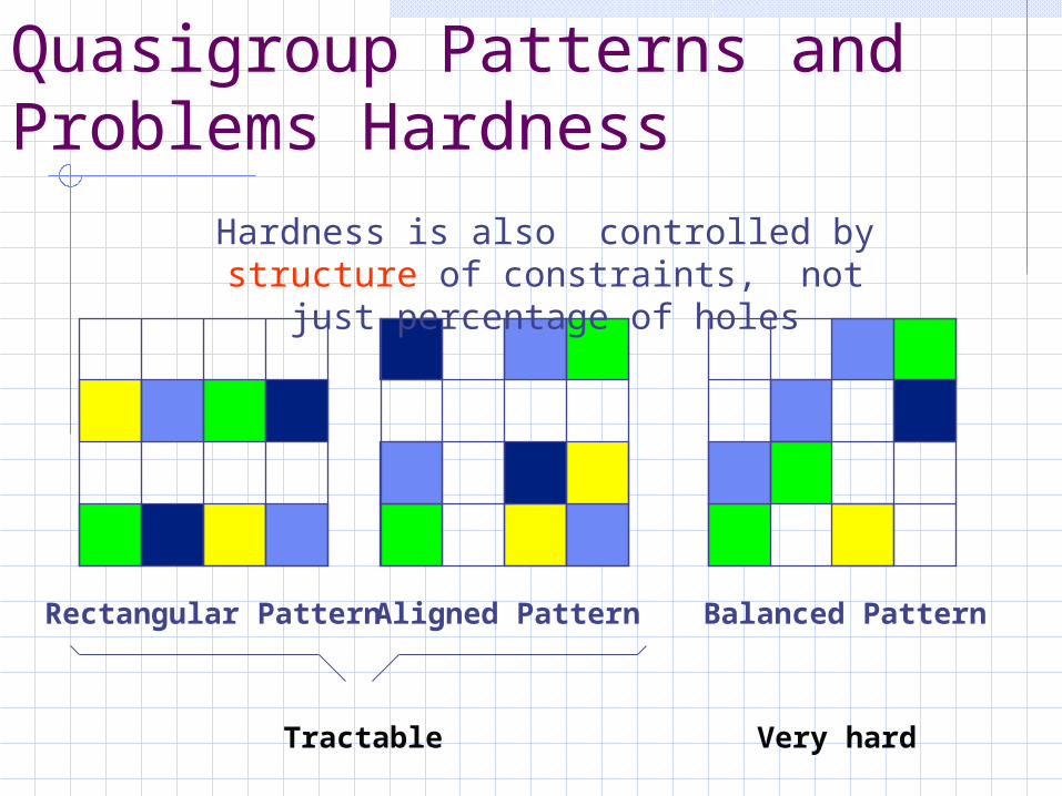
Quasigroup Patterns and Problems Hardness
Rectangular Pattern Aligned Pattern Balanced Pattern
Tractable Very hard
Hardness is also controlled by structure of constraints, not just percentage of holes
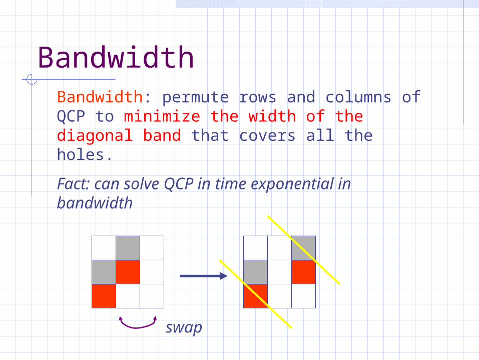
BandwidthBandwidth: permute rows and columns of QCP to minimize the width of the diagonal band that covers all the holes.
Fact: can solve QCP in time exponential in bandwidth
swap

Random vs Balanced
BalancedRandom
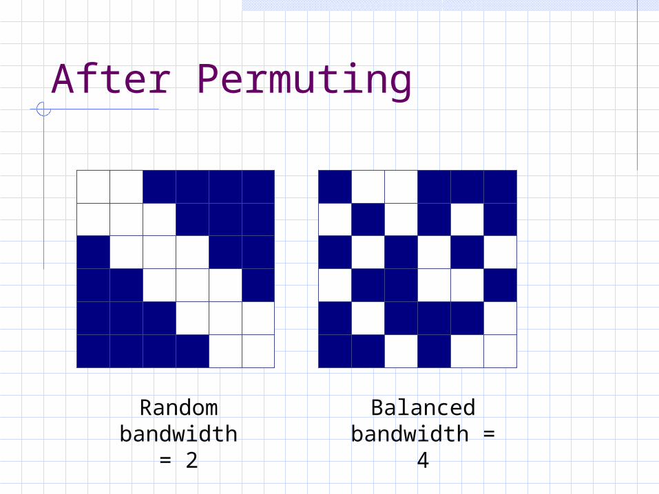
After Permuting
Balanced bandwidth = 4
Random bandwidth = 2
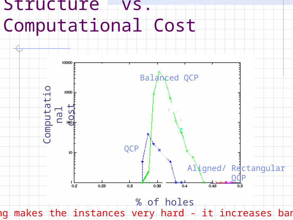
Structure vs. Computational Cost
Balanced QCP
QCP
% of holes
Com
pu
tati
on
al
cost
Balancing makes the instances very hard - it increases bandwith!
Aligned/ Rectangular QCP

Backbone
This instance has4 solutions:
Backbone
Total number of backbone variables: 2
Backbone is the shared structure of all the solutions to a given instance.

Phase Transition in the Backbone (only satisfiable instances)
We have observed a transition in the backbone from a phase where the size of the backbone is around 0% to a phase with backbone of size close to 100%.
The phase transition in the backbone is sudden and it coincides with the hardest problem instances.(Achlioptas, Gomes, Kautz, Selman 00, Monasson et al. 99)
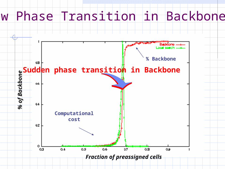
New Phase Transition in Backbone
% Backbone
Sudden phase transition in Backbone
Fraction of preassigned cells
Computationalcost
% o
f B
ackb
on
e
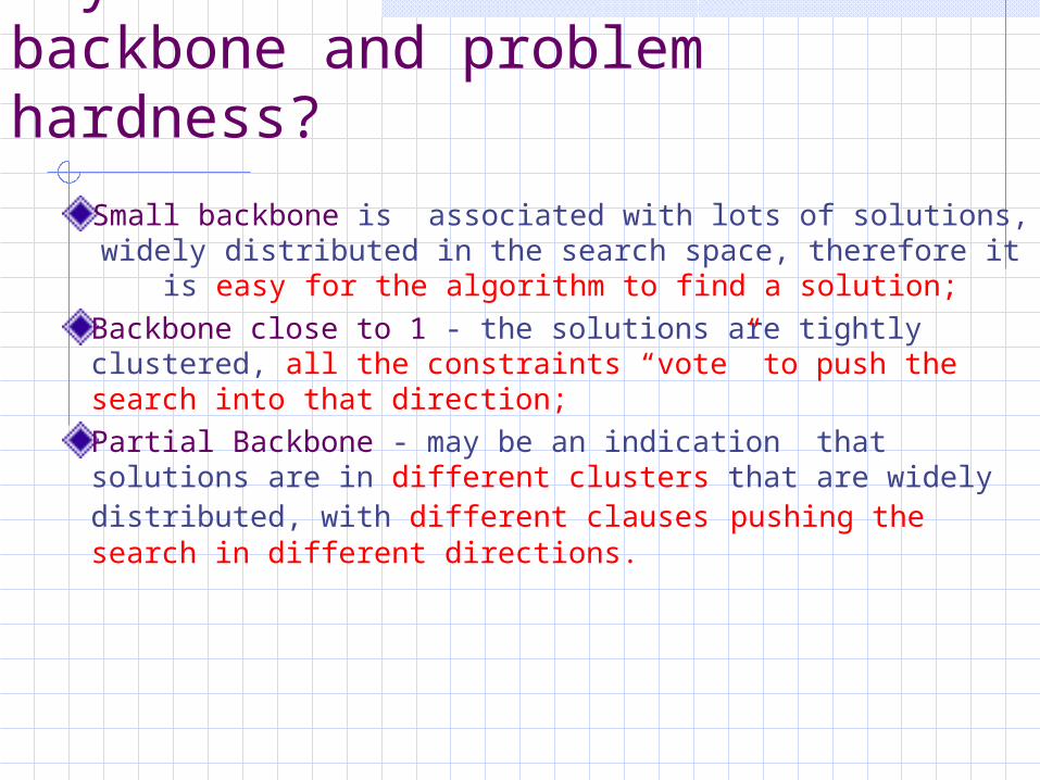
Why correlation between backbone and problem hardness?
Small backbone is associated with lots of solutions, widely distributed in the search space, therefore it is
easy for the algorithm to find a solution;Backbone close to 1 - the solutions are tightly clustered, all the constraints “vote” to push the search into that direction;Partial Backbone - may be an indication that solutions are in different clusters that are widely distributed, with different clauses pushing the search in different directions.
Structural FeaturesStructural Features
The understanding of the structural properties that characterize problem instances such as phase transitions, backbone, balance, and bandwith provides new insights into the practical complexity of computational tasks.
Ant’s Challenge ProblemSensor Domain

ANTs Challenge Problem
Multiple doppler radar sensors track moving targets Energy limited sensors Communication
constraints Distributed
environment Dynamic problem
IISI, Cornell University

Domain Models
Start with a simple graph model Successively refine the model in stages to approximate the real situation: Static weakly-constrained model Static constraint satisfaction model with
communication constraints Static distributed constraint satisfaction model Dynamic distributed constraint satisfaction
model
Goal: Identify and isolate the sources of combinatorial complexity
IISI, Cornell University
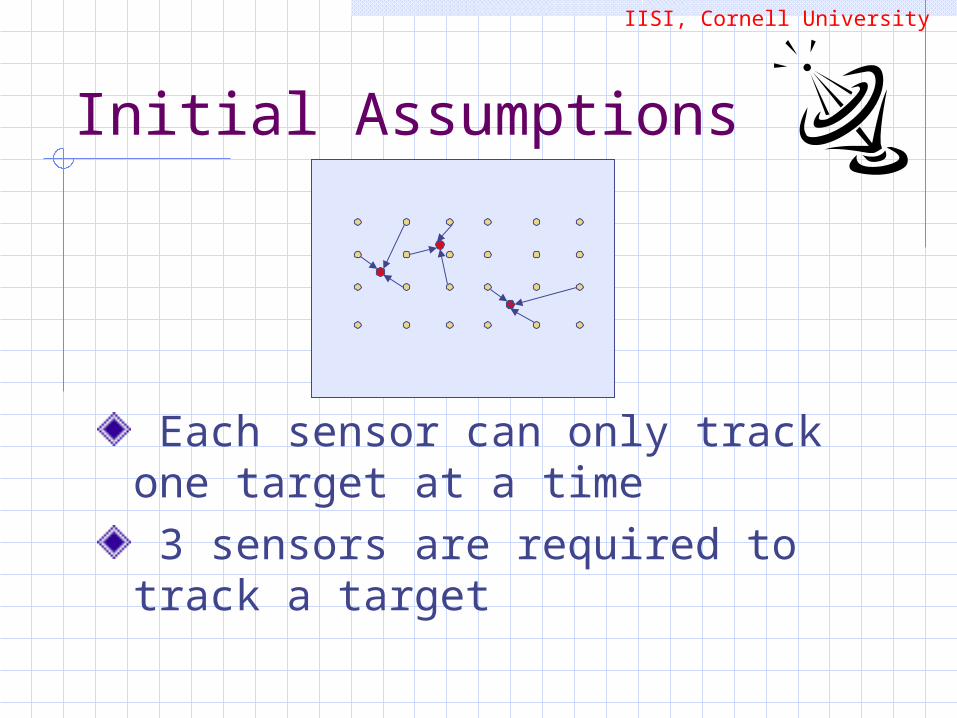
Initial Assumptions
Each sensor can only track one target at a time 3 sensors are required to track a target
IISI, Cornell University
Initial Graph Model
Bipartite graph G = (S U T, E) S is the set of sensor nodes, T the set of target nodes, E the edges indicating which targets are visible to a given sensor Decision Problem: Can each target be tracked by three sensors?
IISI, Cornell University
Initial Graph Model
IISI, Cornell University
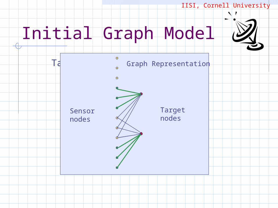
Target visibilityGraph Representation
Sensornodes
Targetnodes
Initial Graph Model
IISI, Cornell University
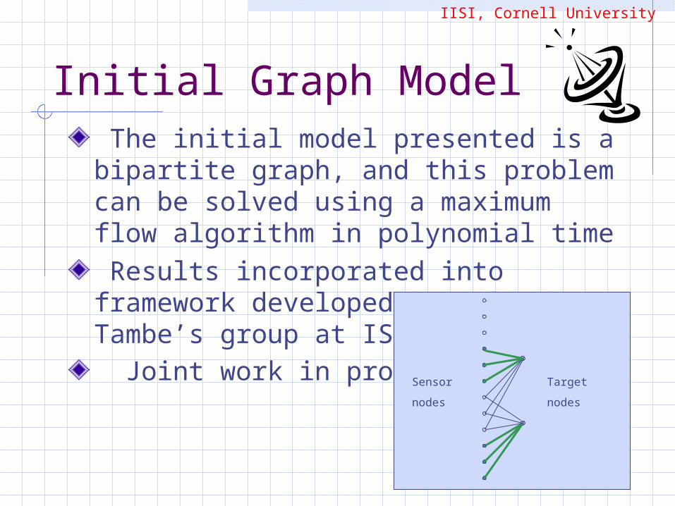
The initial model presented is a bipartite graph, and this problem can be solved using a maximum flow algorithm in polynomial time Results incorporated into framework developed by Milind Tambe’s group at ISI, USC Joint work in progress Sensor
nodes
Target
nodes

Sensor Communication Constraints
IISI, Cornell University
initial modelinitial model + communication edgesinitial model + communication edges
Possible solution
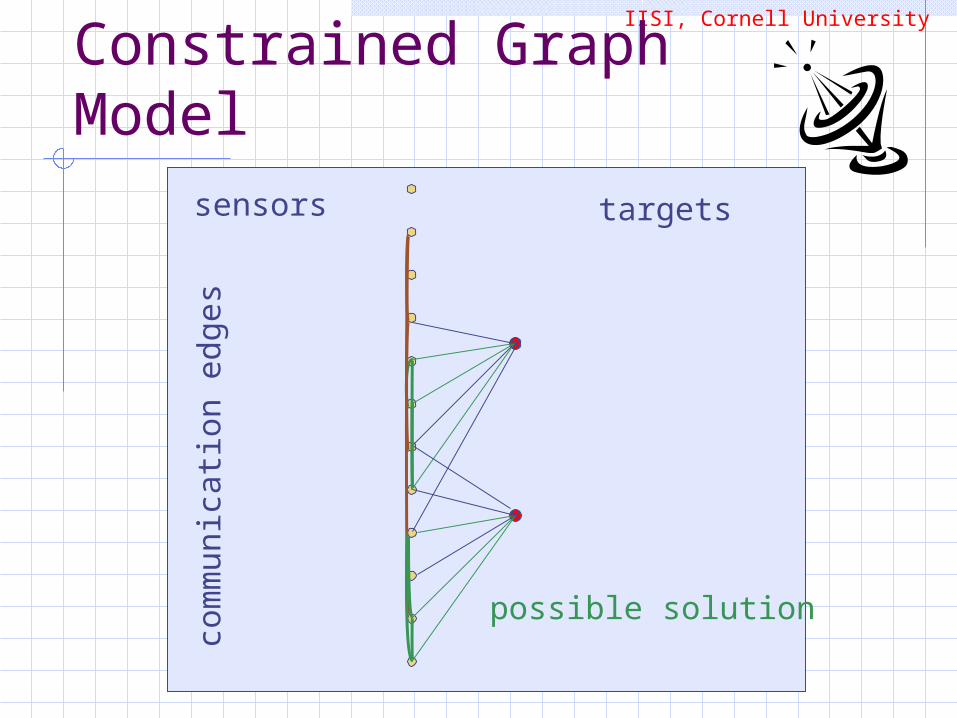
In the graph model, we now have additional edges between sensor nodes
IISI, Cornell University
Constrained Graph Modelsensors targets
com
mu
nic
ati
on e
dg
es
possible solution
Complexity and Phase Transition Phenomena
Complexity
Decision Problem: Can each target be tracked by three sensors which can communicate together ? We have shown that this constraint satisfaction problem (CSP) is NP-complete, by reduction from the problem of partitioning a graph into isomorphic subgraphs
IISI, Cornell University

Average Case complexity and Phase Transition Phenomena
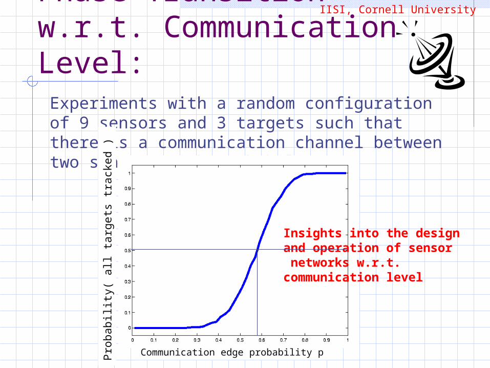
Phase Transition w.r.t. Communication Level:
IISI, Cornell University
Experiments with a random configuration of 9 sensors and 3 targets such that there is a communication channel between two sensors with probability p
Pro
babili
ty(
all
targ
ets
tra
cked )
Communication edge probability p
Insights into the designand operation of sensor networks w.r.t. communication level
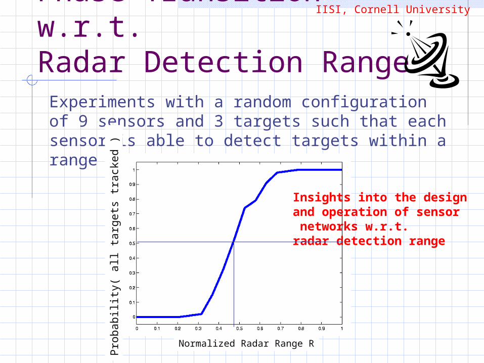
Phase Transition w.r.t. Radar Detection Range
IISI, Cornell University
Experiments with a random configuration of 9 sensors and 3 targets such that each sensor is able to detect targets within a range R
Pro
babili
ty(
all
targ
ets
tra
cked )
Normalized Radar Range R
Insights into the designand operation of sensor networks w.r.t. radar detection range

Distributed Model
Distributed CSP Model
In a distributed CSP (DCSP) variables and constraints are distributed among multiple agents. It consists of: A set of agents 1, 2, … n A set of CSPs P1, P2, … Pn , one for each
agent There are intra-agent constraints and
inter-agent constraints
IISI, Cornell University

DCSP Model
We can represent the sensor tracking problem as DCSP using dual representations: One with each sensor as a distinct
agent One with a distinct tracker agent for
each target
IISI, Cornell University

Sensor AgentsBinary variables associated with each target Intra-agent constraints :
Sensor must track at most 1 visible target
Inter-agent constraints: 3 communicating sensors should track each target
x x0 1s1
s2
s4
t1 t2 t3 t4
s3
x xx 1
1 x0 0
x xx 1

Target Tracker Agents Binary variables associated with each sensorIntra-agent constraints : Each target must be tracked by 3
communicating sensors to which it is visible
Inter-agent constraints: A sensor can only track one target
1 1 x x 10 x xx
x x 1 x xx 1 x1
t1
t2
x x x 1 0x x 11t3
s1 s2 s3 s4 s5 s6 s7 s8 s9
Implicit versus Explicit Constraints
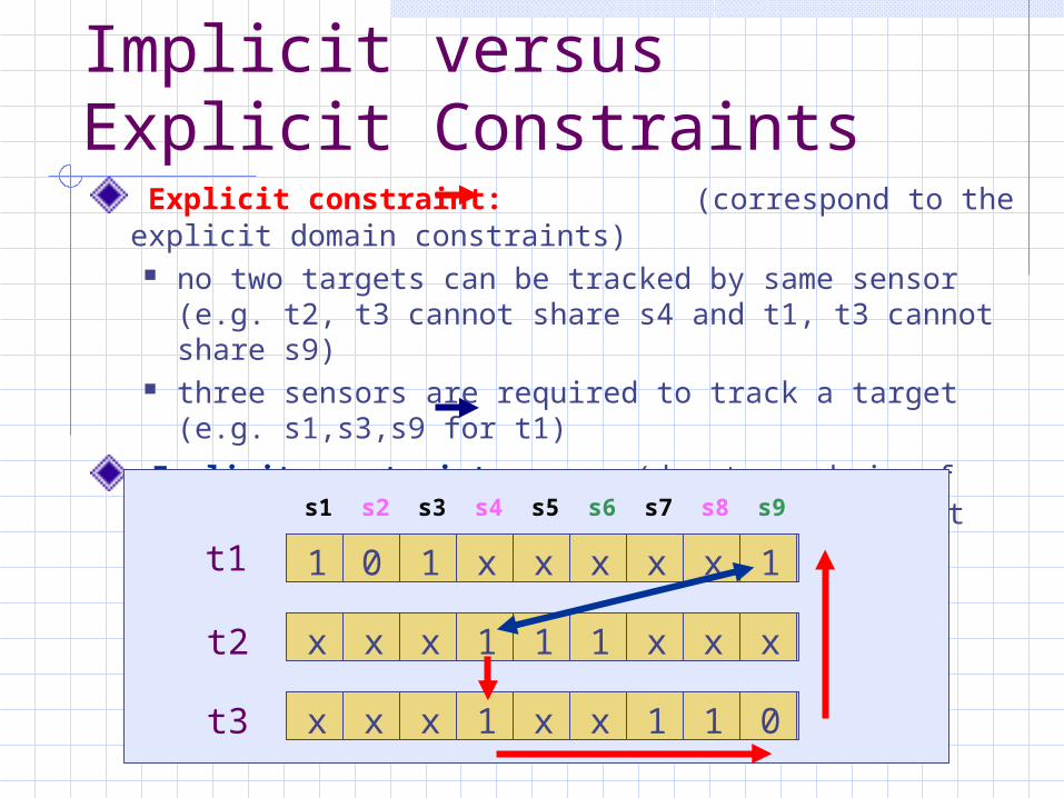
Explicit constraint: (correspond to the explicit domain constraints)
no two targets can be tracked by same sensor (e.g. t2, t3 cannot share s4 and t1, t3 cannot share s9)
three sensors are required to track a target (e.g. s1,s3,s9 for t1)
Implicit constraint: (due to a chain of explicit constraints: (e.g. implicit constraint between s4 for t2 and s9 for t1 )
1 1 x x 10 x xx
x x 1 x xx 1 x1
t1
t2
x x x 1 0x x 11t3
s1 s2 s3 s4 s5 s6 s7 s8 s9
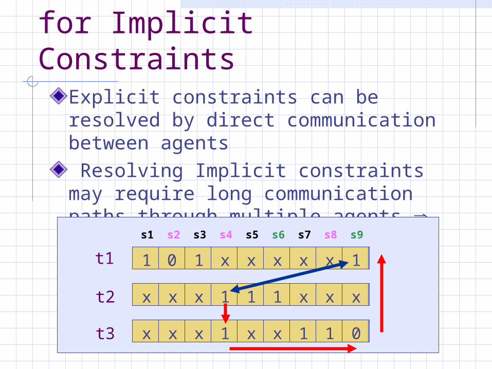
Communication Costs for Implicit Constraints
Explicit constraints can be resolved by direct communication between agents Resolving Implicit constraints may require long communication paths through multiple agents scalability problems
1 1 x x 10 x xx
x x 1 x xx 1 x1
t1
t2
x x x 1 0x x 11t3
s1 s2 s3 s4 s5 s6 s7 s8 s9
Future Work
Structure
Further study structural issues as they occur in the Sensor domain e.g.:
effect of balancing; backbone (insights into critical
resources); refinement of phase transition notions
considering additional parameters;
IISI, Cornell University

DCSP Model
With the DCSP model, we plan to study both per-node computational costs as well as inter-node communication costs
We are in the process of applying known DCSP algorithms to study issues concerning complexity and scalability
IISI, Cornell University
Dynamic DCSP Model
Further refinement of the model: incorporate target mobility The graph topology changes with time What are the complexity issues when online distributed algorithms are involved?
IISI, Cornell University

Summary
Summary
Graph-based models which represent key aspects of the problem domain Results on the complexity of computation and communication for the static model Extensions: additional structural issues on the sensor
domain complexity issues in distributed and dynamic
settings
IISI, Cornell University

Collaborations / Interactions
ISI: Analytic Tools to Evaluate Negotiation Difficulty Design and evaluation of SAT encodings for
CAMERA’s scheduling task.
ISI: DYNAMITE Formal complexity analysis DCSP model (e.g.,
characterization of tractable subclasses).
UMASS: Scalable RT Negotiating Toolkit Analysis of complexity of negotiation
protocols.

The End
IISI, Cornell University
Top Related