


Languages
Pages
Legal

16
Control and Scheduling Software for Flexible Manufacturing Cells
António Ferrolho1, Manuel Crisóstomo2 1Electrical Engineering Department
Superior School of Technology of the Polytechnic Institute of Viseu Campus Politécnico de Repeses, 3504-510 Viseu
PORTUGAL E-mail: [email protected]
2Institute of Systems and Robotics University of Coimbra
Polo II, 3030-290 Coimbra PORTUGAL
E-mail: [email protected]
1. Introduction
One of the most recent developments in the area of industrial automation is the concept of the Flexible Manufacturing Cells (FMC). These are highly computerized systems composed by several types of equipment, usually connected through a Local Area Network (LAN) under some hierarchical Computer Integrated Manufacturing (CIM) structure (Kusiak, 1986) and (Waldner, 1992). FMC are capable of producing a broad variety of products and changing their characteristics quickly and frequently. This flexibility provides for more efficient use of resources, but makes the control of these systems more difficult. Developing an FMC is not an easy task. Usually, an FMC uses equipment (robots, CNC machines, ASRS, etc.) from different manufacturers, having their own programming languages and environments. CNC machines and industrial robots are still machines which are difficult to program, because it is necessary to be knowledgeable in several programming languages and environments. Each manufacturer has a particular programming language and environment (generally local). Robust and flexible control software is a necessity for developing an FMC. We are going to present several software applications developed for industrial robots and CNC machines. The objective of this software is to allow these equipments to be integrated, in an easy and efficient way, in modern Flexible Manufacturing Systems (FMS) and FMC. For the industrial robots we are going to present the “winRS232ROBOTcontrol” and “winEthernetROBOTcontrol” software. For the CNC machines we are going to present the “winMILLcontrol”, for mills, and “winTURNcontrol”, for lathes. With this software, industrial robots and CNC machines can be integrated in modern FMC, in an easy and efficient way. Genetic algorithms (GA) can provide good solutions for scheduling problems. In this chapter we also are going to present a GA to solve scheduling problems in FMC, which
Source: Industrial Robotics: Programming, Simulation and Applicationl, ISBN 3-86611-286-6, pp. 702, ARS/plV, Germany, December 2006, Edited by: Low Kin Huat
Ope
n A
cces
s D
atab
ase
ww
w.i-
tech
onlin
e.co
m
www.intechopen.com
316 Industrial Robotics - Programming, Simulation and Applications
are known to be NP-hard. First, we present a new concept of genetic operators for scheduling problems. Then, we present a developed software tool, called “HybFlexGA” (Hybrid and Flexible Genetic Algorithm), to examine the performance of various crossover and mutation operators by computing simulations of scheduling problems. Finally, the best genetic operators obtained from our computational tests are applied in the “HybFlexGA”. The computational results obtained with 40, 50 and 100 jobs show the good performance and the efficiency of the developed “HybFlexGA” to solving scheduling problems in FMC. An FMC was developed, with industrial characteristics, with the objective of showing the potentialities of the developed software. The use of the “winRS232ROBOTcontrol”, “winEthernetROBOTcontrol”, “winMILLcontrol” and “winTURNcontrol” software allows the coordination, integration and control of FMC. With the “HybFlexGA” software we can solve scheduling problems in FMC. With the work described in this chapter we can:
− Control and monitoring all of the functionalities of the robots and CNC machines remotely. This remote control and monitoring is very important to integrate robots and CNC machines in modern FMS and FMC.
− Develop a distributed software architecture based on personal computers using Ethernet networks.
− Develop applications that allow remote exploration of robots and CNC machines using always the same programming languages (e.g. C++).
− Use a personal computer as programming environment, taking advantage of the huge amount of programming and analysis tools available on these platforms.
− Develop Graphical User Interfaces (GUI) for robots and CNC machines, in a simple and efficient way.
− Write FMS and FMC control software easier, cheaper, and more flexible. As a result, the software expertise resides at the companies and software changes can be made by the company’s engineers. Furthermore, the developed software is easy to modify.
− Control and integrate several equipments from different manufactures in FMS and FMC (e.g. conveyors, motors, sensors, and so on).
− Data sharing. For example: share programmes, share databases and so on, among the client(s) and server(s).
− Solve scheduling problems in FMC with GA.
Suggestions for further research and development work will also be presented.
2. The State of the Art in FMS and FMC Control
An FMS or FMC consists of two major components: hardware and controlling software. The hardware, which includes computer controlled machines (or CNC machines), robots, storage and material handling systems, etc., has been around for decades and problems associated with the hardware have been well studied and are reasonably well understood (Sanjay et al., 1995). But, to write FMS and FMC control software is not a trivial task (Sanjay et al., 1995), (Johi et al., 1991), (Joshi et al., 1995) and (http#1). Nowadays, the software is typically custom written, very expensive, difficult to modify, and often the main source of inflexibility in FMC. Most FMS and FMC are sold to manufacturing
www.intechopen.com

Control and Scheduling Software for Flexible Manufacturing Cells 317
companies as turnkey systems by integration vendors. As a result, the software expertise does not reside at the companies and logic/software changes can only be made by the FMS and FMC vendor. Several references on the use of formal models for automatic generation of software and compilers can be found in the computer literature. The use of formal models for control of flexible manufacturing cells has been discussed by (Sanjay et al., 1995). Other authors (Maimon & Fisher, 1988) have developed rapid software prototyping systems that provide only for the structural specifications of cell control software, still demanding enormous development of hand crafted code to realize effective systems. A detailed description of the implementation of a material handling system as a software/hardware component is given in (Hadj-Alonane et al., 1988).
Research at The Pennsylvania State University’s Computer Integrated Manufacturing
Laboratory (CIMLAB) has been focused on simulation based shop-floor control for more
than a decade and a hierarchical control framework called “RapidCIM” has been
developed. The “RapidCIM” architecture was initially designed for discrete
manufacturing control, and has been implemented using a real-time simulation control
framework. This architecture and its associated tools are capable of automatically
generating much of the necessary software (up to 80 or 90% of a typical application) for
automating discrete manufacturing systems. This substantially reduces the cost of
developing and integrating of such systems, and allows a detailed simulation to be used
for both analyses and control. Information about “RapidCIM” can be found in (Joshi et al.,
1995), (http#1) and (http#2).
3. Industrial Robots Software
Nowadays, the robot controllers working in companies have the following important limitations:
− Some robot controllers only can use RS232 connections and others can support Ethernet networks.
− The robot manipulators have closed controllers and are essentially position-controlled devices that can receive a trajectory and run it continuously.
− Many robot controllers do not allow remote control from an external computer.
− Robot programming environments are not powerful to develop tasks requiring complex control techniques (e.g. integration and control of robots in FMC).
− Robot manipulators from different manufacturers have their own programming language and environments, making the task of integration and cooperation difficult.
To reduce several of these limitations we developed the “winRS232ROBOTcontrol” and the “winEthernetROBOTcontrol”. With these developed software we can:
− Develop a distributed software architecture based on personal computers using Ethernet networks.
− Develop applications that allow remote exploration of robots manipulators using always the same programming languages (e.g. C++).
− Use a personal computer as programming environment, taking advantage of the huge amount of programming and analysis tools available on these platforms.
− Develop Graphical User Interface (GUI), in a simple and efficient way.
www.intechopen.com
318 Industrial Robotics - Programming, Simulation and Applications
3.1 winRS232ROBOTcontrol
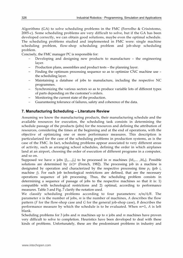
The “winRS232ROBOTcontrol” was developed to be used in robots manipulators where the communication with the controller is only possible through the RS232 serial port. With the “winRS232ROBOTcontrol” it is possible to develop robot programmes in C++, executed at the PC level, not at the robot’s controller level. Nevertheless, the “winRS232ROBOTcontrol” also allows the development of programmes to be executed at a robot’s controller level. Furthermore, it is also possible to have programmes running in the PC and in the robot’s controller (mix solution), individually or simultaneously. The “winRS232ROBOTcontrol” was developed for industrial robot manipulators, and was implemented for the special case of Scorbot ER VII robot. Nevertheless, “winRS232ROBOTcontrol” was designed to work with all robots that support RS232. But, of course, whenever we use a different robot, it is necessary to make some upgrades in the RobotControlAPI library, according to the used robot. The developed API, for the “winRS232ROBOTcontrol” application, is based on a thread process running simultaneously with the main programme. A thread process was created in order to poll the serial port. An event is generated each time data is presented in the serial port. In order to send data to the robot’s controller, the message is placed in the serial port queue. Asynchronous processing will be used to send the message. For example, in order to open the robot’s gripper, a data message is placed in the thread queue and further sent to the robot’s controller trough the RS232 channel. After the delivery of the data, a waiting cycle is activated. This cycle is waiting for the robot’s controller. It ends when the robot’s controller sends back a prompt (‘>’), a timeout error occurs or a cancellation message is sent. Fig. 1 shows the messages cycle of the thread process. The main programme communicates with the parallel process through the messages placed in the waiting queue, being this queue managed by the operating system. A message is immediately processed as soon as it arrives at the parallel process. In the case when there are no messages in the queue, the parallel process enters in a loop, waiting for data from the robot’s controller. An event is generated when data arrive. The parallel process is activated in the beginning of the communication with the controller. When the communication with the robot’s controller is finished, the resources allocated to the parallel process are returned to the operating system.
switch (ReceivedMessage){ case MSG_WAIT: WaitingMessageProcessing(); break case Message1: MessageProcessing1(); break; case Message2: MessageProcessing2(); break; ... case MessageN: MessageProcessingN(); break; default: if(MessageQueueEmpty){ ColocaNaFila(MSG_WAIT); } }
Message processing
loop
MessageN
...
Message2
Message1
Fig. 1. Messages cycle of the parallel process.
www.intechopen.com

Control and Scheduling Software for Flexible Manufacturing Cells 319
The RobotControlAPI library was developed with access to the controller’s functions in mind, as shown in Fig. 2. This API allows us to communicate with the robot’s controller. The available functions are divided into two groups. The first contains public methods and the second contains methods representing events. Table 1 shows some of these functions. We also have developed an Ethernet server for the computer that controls the robot. Thus, it is possible to control the robot remotely, in a distributed client/server environment, as shown in Fig. 2.
RS232
Controller
Robot
RobotControlAPI Open(),Run(),SpeedA(),
Close(),OnMotorsOff(),
…
Ethernet
Client n Client 2 Client 1
...
Ethernet Server
winRS232ROBOTcontrol
Fig. 2. RobotControlAPI library and Ethernet server.
Function Description
SpeedA() Changes group A speed
Home() Homing the robot
MotorsOff() Switches off the robot’s motors
MotorsOn() Switches on the robot’s motors
Close() Closes the gripper
Pu
bli
c
Me
tho
ds
Open() Opens the gripper
OnEndHoming() This event activates after homing
OnClose() This event activates after the execution of the Close() function
OnOpen() This event activates after the execution of the Open() function
OnMotorsOff() This event activates after the motors are switched off
Ev
en
ts
OnMotorsOn() This event activates after the motors are switched on
Table 1. Some available functions.
www.intechopen.com

320 Industrial Robotics - Programming, Simulation and Applications
3.2 winEthernetROBOTcontrol
The “winEthernetROBOTcontrol” was developed to be used in robots manipulators where the communication with the controller is possible through an Ethernet network. The “winEthernetROBOTcontrol” is a Dynamic Link Library (DLL) and allows development of simple and fast applications for robots. The developed software uses the original capabilities of the robot’s controllers, in a distributed client/server environment. Fig. 3 shows the PC1 and PC4 communicating with the robots through “winEthernetROBOTcontrol”.
...
Ethernet
winEthernetROBOTcontrol
PC1 PC4
Robot BRobot A
ControllerController
Client n Client 2 Client 1
...
Ethernet
Server
Ethernet
Server
Fig. 3. winEthernetROBOTcontrol.
Description
Robot() Add New Alias
S4ProgamLoad() Load a programme in the robot controller
S4Run() Switches ON the robot’s motors
S4Standby() Switches OFF the robot’s motors
S4Start() Start programme execution
S4Stop() Stop programme execution
S4ProgramNumVarRead() Reads a numerical variable in the robot controller
S4ProgramNumVarWrite() Writes a numerical variable in the robot controller
S4ProgramStringVarWrite() Writes a string in the robot controller
Pro
ced
ure
s
S4ProgramStringVarRead() Reads a string in the robot controller
Add_Variable() Add a new variable
Remove_Variable() Remove one variable
ControlID() Gives the ID controller
Fu
nct
ion
s
InerfaceState() Gives the interface state.
StatusChanged() This event activates after something changed in the robot controller. For example: power off, emergency stop, executing sate, stopped state, run, and so on.
BoolVariableChanged() This event activates after one Boolean variable changed Ev
en
ts
NumVariableChanged() This event activates after one numeric variable changed
Table 2. Some available procedures, functions and events.
www.intechopen.com

Control and Scheduling Software for Flexible Manufacturing Cells 321
Table 2 presents same procedures, functions and events developed for the
“winEthernetROBOTcontrol”. The procedure “Robot” allows making a connection between one
PC (with winEthernetROBOTcontrol) and one or more robots. For that, it is necessary to create
and configure one connection between the PC and the robot controller (Add New Alias). After
that it is possible to communicate and control the robot remotely through the connection (Alias).
With “winEthernetROBOTcontrol” we can develop a software control, for one or more
robots, in any PC. With this PC we can communicate and control the robot (or robots)
through an Ethernet (see Fig. 3).
The “winEthernetROBOTcontrol” library was developed for industrial robot manipulators, and
was implemented for the special case of ABB robots (with the new S4 control system).
Nevertheless, this very flexible library was designed to work with all robots that support Ethernet.
But, of course, if we use a different robot it is necessary to make some upgrades in this library,
according to the used robot. The basic idea is to define a library of functions for any specific
equipment that in each moment define the basic functionality of that equipment for remote use.
4. Industrials CNC Machines Software
Nowadays, all the manufactured CNC machines support Ethernet networks. But, these actual CNC machines have the following important limitations:
− The actual CNC machines have closed numerical control (NC) and are developed to work individually, not integrated with others equipments (e.g. others machines, robots, and so on).
− Actual CNC machine’s controllers do not allow remote control from an external computer.
− CNC machine’s programming environments are not powerful enough to develop tasks requiring complex control techniques (e.g. integration and control CNC machines in FMC).
− CNC machines from different manufacturers have their own programming language and environments, making the task of integration and cooperation difficult.
To reduce these limitations, we developed two programmes in C++ that allow controlling the CNC machines through Direct Numerical Control (DNC). For lathes, the “winTURNcontrol” programme was developed, and “winMILLcontrol” for mills. With the proposed software we can reduce several limitations in CNC machines:
− We can control and monitor all of the functionalities of the CNC machines remotely (e.g. open and close door, open and close chuck, open and close vice, start machine, machine ready, and so on). This control and monitoring remotely is very important to integrate CNC machines in modern FMS and FMC.
− We can develop a distributed software architecture based on personal computers using Ethernet networks.
− We can develop applications that allow remote exploration of CNC machines using always the same programming languages (e.g. C++).
− We can use a personal computer as programming environment, taking advantage of the huge amount of programming and analysis tools available on these platforms.
www.intechopen.com

322 Industrial Robotics - Programming, Simulation and Applications
− We can develop Graphical User Interface (GUI) for CNC machines, in a simple and efficient way.
Some CNC machine’s controllers (e.g. FANUC) only allow external connections through the RS232 serial port (Ferrolho et al., 2005). In order to surpass this limitation, a “Null Modem” cable was connected between COM1 and COM2 serial port of each PC that controls the respective machine, as shown in Fig. 4. The developed DNC programmes use the COM1 to send orders (e.g. open door, close vice, start NC programme, and so on) to the machine and the CNC machine’s controllers receive the same orders by COM2. For that, we need configure the CNC machines software to receive the DNC orders by COM2. We have developed an Ethernet server for the PCs that control the machines, so as to allow remote control of the machines. Thus, it is possible to control the machines remotely, as shown in Fig. 4. Each machine’s server receives the information through the Ethernet and then sends it to the machine’s controller through the serial port. For example, if the client 1, in Fig. 4, needs to send an order (e.g. close door) to the machine A, the developed programme running in the machine computer receives the order through the Ethernet and sends the same order to the COM1 port. After that, the machine’s controller receives this order through the COM2 (null modem cable) and then the machine closes the door. DNC is an interface that allows a computer to control and monitor one or more CNC machines. The DNC interface creates a connection between client (e.g. client 1) and the CNC machine computer. After activating the DNC mode, client starts to control the CNC machines through the Ethernet, as shown in Fig. 4. The developed DNC interface establishes a TCP/IP connection between computer client and the CNC machine’s computer. With the DNC interface developed it is possible to perform the following remotely: transfer NC programmes (files of NC codes) to the CNC machines, work with different parts’ NC files, visualize alarms and information regarding the state of the CNC machines, control all the devices of the CNC machines (e.g. doors, clamping devices, blow-out, refrigeration system, position tools, auxiliary drives, and so on).
Ethernet
Client n Client 1
...
Machine A
COM1
COM2
Ethernet Server
...
Machine C
COM1
COM2
Ethernet Server
COM1
COM2
Ethernet Server
Machine B
Client 2
Fig. 4. Control CNC machines through Ethernet.
www.intechopen.com

Control and Scheduling Software for Flexible Manufacturing Cells 323
5. USB software and USB Kit
We have developed hardware (USB Kit) and software (USB software) for control and integration of several equipments in FMS and FMC (e.g. conveyors, motors, sensors, actuators, and so on). The USB Kit has various inputs and outputs where we can connect various sensors and actuators from different manufacturers. The communication between the PC1 and USB Kit is done by USB port, as shown in Fig. 5. The PC1 communicates with others PCs through Ethernet.
Ethernet
…
PC1
...
Hardware
USB Kit
Inputs / Outputs
USB Software
USB
Communication
Client n Client 1
...Client 2
Ethernet Server
Fig. 5. USB software and USB kit.
6. Developed Flexible Manufacturing Cell
The developed FMC is comprised of four sectors and the control of existing equipment in each sector is carried out by four computers: PC1 – manufacturing sector, PC2 – assembly sector, PC3 – handling sector and PC4 – storage sector. The coordination, synchronization and integration of the four sectors is carried out by the FMC manager computer. The four sectors are (Ferrolho & Crisóstomo, 2005-a) and (Ferrolho & Crisóstomo, 2005-b):
− The manufacturing sector, made up of two CNC machines (mill and lathe), one ABB IRB140 robot and one buffer.
− The assembly sector, made up of one Scorbot ER VII robot, one small conveyor and an assembly table.
www.intechopen.com

324 Industrial Robotics - Programming, Simulation and Applications
− The handling sector, made up of one big conveyor.
− The storage sector, made up of five warehouses and one robot ABB IRB1400.
The hierarchical structure implemented in the FMC is shown in Fig. 6. In the FMC three communication types were used: Ethernet in the manufacturing sector and storage sector, RS232 in the assembly sector and USB in the handling sector. PC1, PC2, PC3, PC4 and FMC manager PC are connected via Ethernet as shown in Fig. 6. If necessary it is possible to develop new applications using other communication types.
Manufacturing sector
Assembly sector
Storage sector
Handling sector
ABB robot IRB 140
Ethernet
ABB IRB140 robot
ABB IRB1400 robot
Server software
PC1
Software
“Manufacturing Sector”
PC2 PC3 PC4
Software
“Assembly sector”
ABB robot IRB 140
Controller
Scorbot
Scorbot ER VII
Big conveyor
Hardware
Kit USB
Storage
sector
DB
Software
“Handling sector”
Software
“Storage sector”
Fifth layer
Data
acquisition
Fourth layer
Control
First layer
Engineering
Third layer
Scheduling
Second layer
Planning
Server software
The software developed for this PC allows:
- Coordination, integration and control all the
sectors in FMC.
- Control and supervision in real time all the
operation in FMC.
- Maintaining a database of jobs to
manufacture, including the respective NC
programmes.
- Synchronizing the various sectors to produce
variable lots of different types of parts
depending on the customer’s orders.
- Monitoring the current state of the
production.
(cont.)
- Guaranteeing tolerance of failures, safety
and coherence of the data.
- Developing and designing new products to
manufacture – the engineering layer.
- Production plans, assemblies and product
tests – the planning layer.
- Finding the optimum processing sequence to
optimize CNC machine use – the
scheduling layer.
FMC Manager PC
Small conveyor
Manufacturing
jobs
DB
CNC Lathe
CNC Mill
Lathe Buffer
Controller
S4Cplus
Mill Buffer
Machine state and send
Commands by DNC software
win
MIL
Lco
ntr
ol Robot state and send commands by
“winEthernetROBOTcontrol”
win
Eth
ernet
RO
BO
Tco
ntr
ol
win
RS
232
RO
BO
Tco
ntr
ol
win
Eth
ern
etR
OB
OT
con
trol
US
B
com
mu
nic
atio
n
RS
23
2
com
mun
icat
ion
US
B S
oft
war
e
win
TU
RN
contr
ol
Fig. 6. Hierarchical structure of FMC.
The layered level of the proposed architecture has inherent benefits. This hierarchical structure allows adding new sectors in the FMC, in an easy and efficient way. The new sectors can also use several equipments from different manufacturers. For this, we only need to add a computer in the fourth layer and to develop software to control the several equipments in those sectors.
www.intechopen.com

Control and Scheduling Software for Flexible Manufacturing Cells 325
Manufacturing Sector
Control of the manufacturing sector is carried out by the PC1, as shown in Fig. 6. The manufacturing sector is controlled by software, developed in C++, and has the following functions: buffer administration, CNC machine administration and ABB IRB140 robot control. Control of the IRB140 robot is carried out by “winEthernetROBOTcontrol”. Control of the Mill and Lathe is carried out by DNC software – “winMILLcontrol” and “winTURNcontrol” (Ferrolho et al., 2005). This software has a server which allows remote control of the manufacturing sector.
Assembly Sector
The assembly sector is made up of a Scorbot ER VII robot, a conveyor and an assembly table, as shown in Fig. 6. Responsibility for the control and coordination of this sector falls on PC2 and in this sector we used the “winRS232ROBOTcontrol”.
Handling Sector
Control of the handling sector is carried out through the PC3 and of a USB kit (hardware), as shown in Fig. 6. The USB kit acquires the signals coming from the sensors and sends them to PC3. When it is necessary to activate the stoppers, PC3 sends the control signals to the USB kit.
Storage Sector
Control of the storage sector is carried out by PC4, as shown in Fig. 6. The functions of the developed software are the administration of the database of the whole warehouse, and controlling the ABB IRB1400 robot. The database can be updated at any moment by the operator, but it is also automatically updated whenever the ABB IRB1400 robot conducts a load operation, unloads or replaces pallets. Control of the ABB 1400 robot is carried out by “winEthernetROBOTcontrol” functions, procedures and events.
FMC Manager PC
The central computer (FMC manager PC) controls all of the FMC production, connecting the various computers and data communication networks, which allows real time control and supervision of the operations, collecting and processing information flow from the various resources. In this PC the first three layers of the hierarchical structure presented in Fig. 6 are implemented: engineering, planning and scheduling. The first layer contains the engineering and product design, where the product is designed and developed with CAD/CAM software (e.g. MasterCam). The outputs of this layer are the drawings and the bill of materials. The second layer is process planning. Here the process plans for manufacturing, assembling and testing are made. The outputs of this layer are the NC code for the CNC machines. We can obtain these NC code also with CAD/CAM software. After that we put the product design, process plan, NC code, and so on, of each job in the products database. Whenever we have a new product (job) it is necessary to put all the information about this job in the products database. The third layer is scheduling. The process plans together with the drawing, the bill of materials and the customer orders are the input to scheduling. The output of scheduling is the release of the order to the manufacturing floor. We used Genetic
www.intechopen.com
326 Industrial Robotics - Programming, Simulation and Applications
Algorithms (GA) to solve scheduling problems in the FMC (Ferrolho & Crisóstomo, 2005-c). Some scheduling problems are very difficult to solve, but if the GA has been developed correctly, we can obtain good solutions, maybe even the optimal schedule. The scheduling problems studied and implemented in FMC were: single machine scheduling problem, flow-shop scheduling problem and job-shop scheduling problem. Concisely, the FMC manager PC is responsible for:
− Developing and designing new products to manufacture – the engineering layer.
− Production plans, assemblies and product tests – the planning layer.
− Finding the optimum processing sequence so as to optimize CNC machine use – the scheduling layer.
− Maintaining a database of jobs to manufacture, including the respective NC programmes.
− Synchronizing the various sectors so as to produce variable lots of different types of parts depending on the customer’s orders.
− Monitoring the current state of the production.
− Guaranteeing tolerance of failures, safety and coherence of the data.
7. Manufacturing Scheduling – Literature Review
Assuming we know the manufacturing products, their manufacturing schedule and the available resources for execution, the scheduling task consists in determining the schedule passage of the products (jobs) for the resources and defining the attribution of resources, considering the times at the beginning and at the end of operations, with the objective of optimizing one or more performance measures. This description is particularized for the case of the scheduling problems in production systems, as is the case of the FMC. In fact, scheduling problems appear associated to very different areas of activity, such as arranging school schedules, defining the order in which airplanes land at an airport, choosing the order of execution of different programs in a computer, and so on. Supposed we have n jobs {J1,...,Jn} to be processed in m machines {M1,... ,Mm}. Possible solutions are determined by (n!)m (French, 1982). The processing job in a machine is designated by operation and characterized by the respective processing time pij (job i, machine j). For each job technological restrictions are defined, that are the necessary operations sequence of job processing. Thus, the scheduling problem consists in determining a sequence of passage of jobs to the respective machines so that it is: 1) compatible with technological restrictions and 2) optimal, according to performance measures. Table 3 and Fig. 7 clarify the notation used. We classify scheduling problems according to four parameters: n/m/A/B. The parameter n is the number of jobs, m is the number of machines, A describes the flow pattern (F for the flow-shop case and G for the general job-shop case), B describes the performance measure by which the schedule is to be evaluated. When m=1, A is left blank. Scheduling problems for 3 jobs and m machines up to n jobs and m machines have proven very difficult to solve to completion. Heuristics have been developed to deal with these kinds of problems. Unfortunately, these are the predominant problems in industry and
www.intechopen.com

Control and Scheduling Software for Flexible Manufacturing Cells 327
therefore computationally efficient techniques are very important for their solution. Some of the problems are made even more difficult when the rate of demand for products varies. This dynamic element violates some of the convenient assumptions about approaches used in static cases (Rembold et al., 1993).
Description Symbol Remarks
Number of jobs n
Job i Ji
Machine j Mj
Operation time Oij
Processing time pij
Read time for Ji ri
Due date for Ji di
Allowance for Ji ai ai=di-ri
Waiting time of Ji preceding the respective k th operation
Wik
Total waiting time of Ji Wi ∑=
=m
k
iki WW1
Completion time of Ji Ci [ ]∑=
++=m
k
kijikii pWrC1
)(
Flow time of Ji Fi Fi=Ci-ri
Lateness of Ji Li Li=Ci-di
Tardiness of Ji Ti Ti=max{0, Li}
Earliness of Ji Ei Ei=max{-Li, 0}
Idle time on machine Mj Ij ∑=
−=n
i
ijj pCI1
max
Table 3. Scheduling notation.
As stated, the general n jobs and m machines job-shop scheduling problem has proved to be very difficult. The difficult is not in modeling but in computation since there is a total of (n!)m possible schedules, and each one must be examined to select the one that gives the minimum makespan or optimizes whatever measure of effectiveness is chosen. There are no known efficient, exact solution procedures. Some authors have formulated integer programming models but the computational results (computational complexity) have not been encouraging. For small problems, the branch and bound technique has been shown to be very good and better than integer programming formulation, but this has been computationally prohibitive for large problems. In the next sections we are going to present a GA to solve scheduling jobs in FMC. First, we present a new concept of genetic operators. Then, we present a developed software tool “HybFlexGA”. Finally, we show the good performance and the efficiency of the developed “HybFlexGA” to solving scheduling problems in FMC.
8. Genetic Algorithms
The strong performance of the GA depends on the choice of good genetic operators. Therefore, the selection of appropriate genetic operators is very important for
www.intechopen.com

328 Industrial Robotics - Programming, Simulation and Applications
constructing a high performance GA. Various crossover and mutation operators have been examined for sequencing problems in the literature (for example, see (Goldberg, 1989), (Oliver et al., 1987), (Syswerda, 1991), (Ferrolho & Crisóstomo, 2005-d) and (Murata & Ishibuchi, 1994)). When the performance of a crossover operator is evaluated, a GA without mutation is employed and the evaluation of a mutation operator is carried out by a GA without crossover. In the literature, various crossover operators and mutation operators were examined in this manner (for example, see (Murata & Ishibuchi, 1994)). In this section, we propose a new concept of genetic operators for scheduling problems. We evaluate each of various genetic operators with the objective of selecting the best performance crossover and mutation operators.
Oij(3)
Wi2 pij(2)
...
Oij(2)
Wim pij(m)
Oij(m-1)
...
Oij(m-1)
...
M1
M2
Mj
...
... Oij(m)
...
pij(1)
Oij(1)
...
M(m-1)
...
Mm
...
ri di
Ci
Fi
ai Li
Fig. 7. Gantt diagram of a typical job Ji.
8.1 Crossover Operators
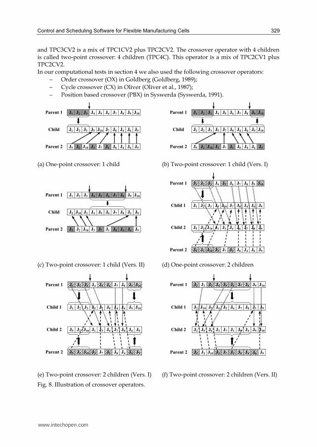
Crossover is an operation to generate a new sequence (child chromosome) from two sequences (parent chromosomes). We developed the following crossover operators:
− One-point crossover: 1 child (OPC1C) in Fig. 8 a).
− Two-point crossover: 1 child (Version I) (TPC1CV1) in Fig. 8 b).
− Two-point crossover: 1 child (Version II) (TPC1CV2) in Fig. 8 c).
− One-point crossover: 2 children (OPC2C) in Fig. 8 d).
− Two-point crossover: 2 children (Version I) (TPC2CV1) in Fig. 8 e).
− Two-point crossover: 2 children (Version II) (TPC2CV2) in Fig. 8 f). We also developed crossover operators with 3 and 4 children. The crossover operators with 3 children are called two-point crossover: 3 children (Version I) (TPC3CV1) and two-point crossover: 3 children (Version II) (TPC3CV2). TPC3CV1 is a mix of TPC1CV1 plus TPC2CV1
www.intechopen.com
Control and Scheduling Software for Flexible Manufacturing Cells 329
and TPC3CV2 is a mix of TPC1CV2 plus TPC2CV2. The crossover operator with 4 children is called two-point crossover: 4 children (TPC4C). This operator is a mix of TPC2CV1 plus TPC2CV2. In our computational tests in section 4 we also used the following crossover operators:
− Order crossover (OX) in Goldberg (Goldberg, 1989);
− Cycle crossover (CX) in Oliver (Oliver et al., 1987);
− Position based crossover (PBX) in Syswerda (Syswerda, 1991).
Parent 1 J1 J2 J3 J4 J5 J6 J7 J8 J9 J10
Child J1 J2 J3 J5 J10 J7 J8 J4 J6 J9
Parent 2 J5 J2 J10 J3 J7 J1 J8 J4 J6 J9
Parent 1 J1 J2 J3 J4 J5 J6 J7 J8 J9 J10
Child J1 J2 J3 J5 J7 J8 J4 J6 J9 J10
Parent 2 J5 J2 J10 J3 J7 J1 J8 J4 J6 J9
(a) One-point crossover: 1 child (b) Two-point crossover: 1 child (Vers. I)
Parent 1 J1 J2 J3 J4 J5 J6 J7 J8 J9 J10
Child J2 J10 J3 J4 J5 J6 J7 J8 J1 J9
Parent 2 J5 J2 J10 J3 J7 J1 J8 J4 J6 J9
Parent 1 J1 J2 J3 J4 J5 J6 J7 J8 J9 J10
Child 1 J1 J2 J3 J5 J10 J7 J8 J4 J6 J9
Child 2 J5 J2 J10 J1 J3 J4 J6 J7 J8 J9
Parent 2 J5 J2 J10 J3 J7 J1 J8 J4 J6 J9
(c) Two-point crossover: 1 child (Vers. II) (d) One-point crossover: 2 children
Parent 1 J1 J2 J3 J4 J5 J6 J7 J8 J9 J10
Child 1 J1 J2 J3 J5 J7 J8 J4 J6 J9 J10
Child 2 J5 J2 J10 J1 J3 J4 J7 J8 J6 J9
Parent 2 J5 J2 J10 J3 J7 J1 J8 J4 J6 J9
Parent 1 J1 J2 J3 J4 J5 J6 J7 J8 J9 J10
Child 1 J2 J10 J3 J4 J5 J6 J7 J8 J1 J9
Child 2 J2 J5 J6 J3 J7 J1 J8 J4 J9 J10
Parent 2 J5 J2 J10 J3 J7 J1 J8 J4 J6 J9
(e) Two-point crossover: 2 children (Vers. I) (f) Two-point crossover: 2 children (Vers. II)
Fig. 8. Illustration of crossover operators.
www.intechopen.com
330 Industrial Robotics - Programming, Simulation and Applications
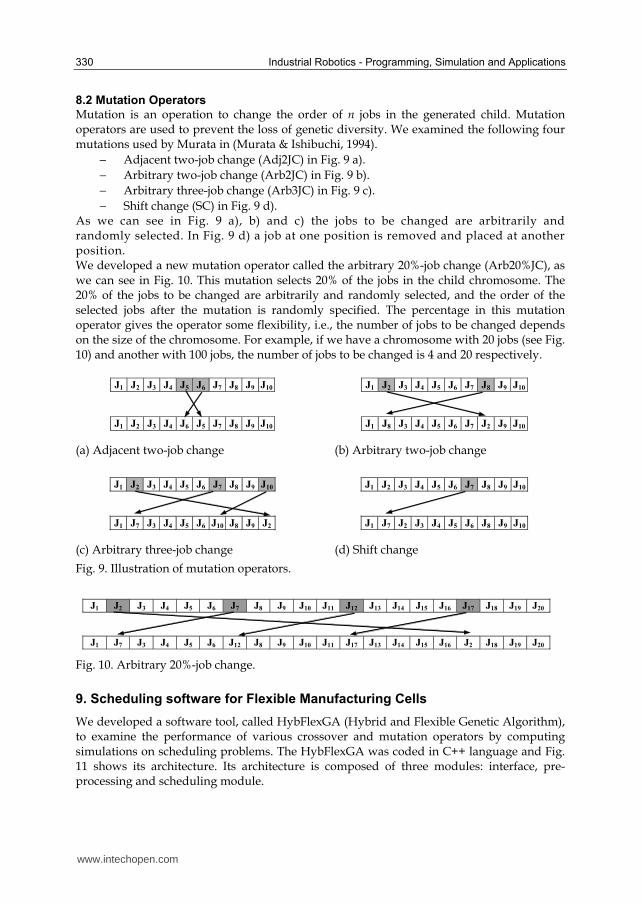
8.2 Mutation Operators
Mutation is an operation to change the order of n jobs in the generated child. Mutation operators are used to prevent the loss of genetic diversity. We examined the following four mutations used by Murata in (Murata & Ishibuchi, 1994).
− Adjacent two-job change (Adj2JC) in Fig. 9 a).
− Arbitrary two-job change (Arb2JC) in Fig. 9 b).
− Arbitrary three-job change (Arb3JC) in Fig. 9 c).
− Shift change (SC) in Fig. 9 d). As we can see in Fig. 9 a), b) and c) the jobs to be changed are arbitrarily and randomly selected. In Fig. 9 d) a job at one position is removed and placed at another position. We developed a new mutation operator called the arbitrary 20%-job change (Arb20%JC), as we can see in Fig. 10. This mutation selects 20% of the jobs in the child chromosome. The 20% of the jobs to be changed are arbitrarily and randomly selected, and the order of the selected jobs after the mutation is randomly specified. The percentage in this mutation operator gives the operator some flexibility, i.e., the number of jobs to be changed depends on the size of the chromosome. For example, if we have a chromosome with 20 jobs (see Fig. 10) and another with 100 jobs, the number of jobs to be changed is 4 and 20 respectively.
J1 J2 J3 J4 J5 J6 J7 J8 J9 J10
J1 J2 J3 J4 J6 J5 J7 J8 J9 J10
J1 J2 J3 J4 J5 J6 J7 J8 J9 J10
J1 J8 J3 J4 J5 J6 J7 J2 J9 J10
(a) Adjacent two-job change (b) Arbitrary two-job change
J1 J2 J3 J4 J5 J6 J7 J8 J9 J10
J1 J7 J3 J4 J5 J6 J10 J8 J9 J2
J1 J2 J3 J4 J5 J6 J7 J8 J9 J10
J1 J7 J2 J3 J4 J5 J6 J8 J9 J10
(c) Arbitrary three-job change (d) Shift change
Fig. 9. Illustration of mutation operators.
J1 J2 J3 J4 J5 J6 J7 J8 J9 J10 J11 J12 J13 J14 J15 J16 J17 J18 J19 J20
J1 J7 J3 J4 J5 J6 J12 J8 J9 J10 J11 J17 J13 J14 J15 J16 J2 J18 J19 J20
Fig. 10. Arbitrary 20%-job change.
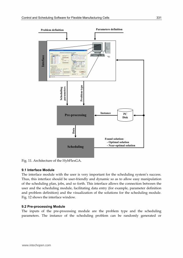
9. Scheduling software for Flexible Manufacturing Cells
We developed a software tool, called HybFlexGA (Hybrid and Flexible Genetic Algorithm), to examine the performance of various crossover and mutation operators by computing simulations on scheduling problems. The HybFlexGA was coded in C++ language and Fig. 11 shows its architecture. Its architecture is composed of three modules: interface, pre-processing and scheduling module.
www.intechopen.com
Control and Scheduling Software for Flexible Manufacturing Cells 331
Instance
Sch
ed
uli
ng
pa
ra
mete
rs
Inte
face
Problem definition Parameters definition
Found solution:
- Optimal solution
- Near-optimal solution
Da
ta
Pro
ble
m t
yp
e
Pre-processing
Scheduling
PC
Disk
Fig. 11. Architecture of the HybFlexGA.
9.1 Interface Module
The interface module with the user is very important for the scheduling system’s success.
Thus, this interface should be user-friendly and dynamic so as to allow easy manipulation
of the scheduling plan, jobs, and so forth. This interface allows the connection between the
user and the scheduling module, facilitating data entry (for example, parameter definition
and problem definition) and the visualization of the solutions for the scheduling module.
Fig. 12 shows the interface window.
9.2 Pre-processing Module
The inputs of the pre-processing module are the problem type and the scheduling
parameters. The instance of the scheduling problem can be randomly generated or
www.intechopen.com
332 Industrial Robotics - Programming, Simulation and Applications
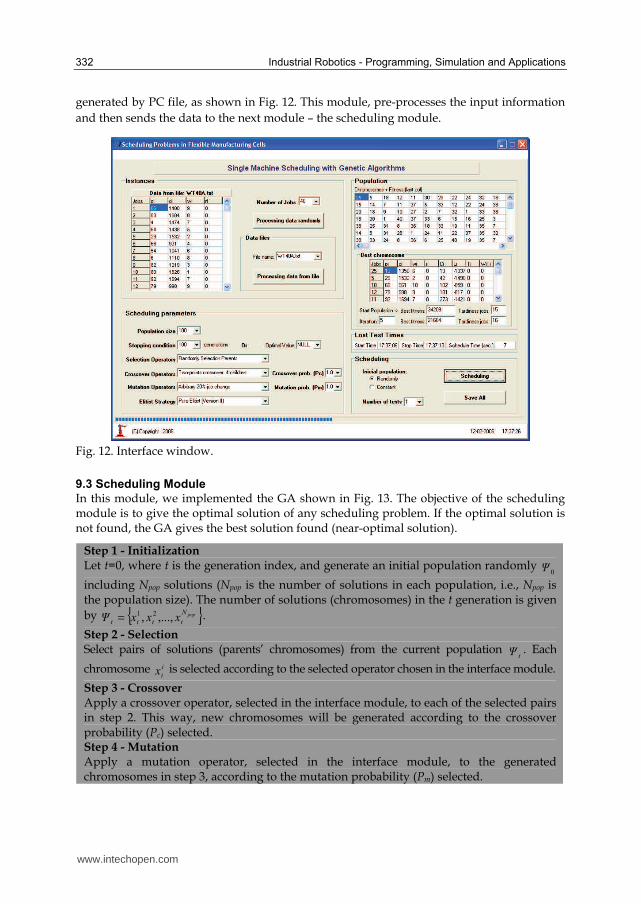
generated by PC file, as shown in Fig. 12. This module, pre-processes the input information
and then sends the data to the next module – the scheduling module.
Fig. 12. Interface window.
9.3 Scheduling Module
In this module, we implemented the GA shown in Fig. 13. The objective of the scheduling module is to give the optimal solution of any scheduling problem. If the optimal solution is not found, the GA gives the best solution found (near-optimal solution).
Step 1 - Initialization Let t=0, where t is the generation index, and generate an initial population randomly
0Ψ
including Npop solutions (Npop is the number of solutions in each population, i.e., Npop is the population size). The number of solutions (chromosomes) in the t generation is given
by { }popN
tttt xxxΨ ,...,, 21= .
Step 2 - Selection Select pairs of solutions (parents’ chromosomes) from the current population
tΨ . Each
chromosome i
tx is selected according to the selected operator chosen in the interface module.
Step 3 - Crossover Apply a crossover operator, selected in the interface module, to each of the selected pairs in step 2. This way, new chromosomes will be generated according to the crossover probability (Pc) selected. Step 4 - Mutation Apply a mutation operator, selected in the interface module, to the generated chromosomes in step 3, according to the mutation probability (Pm) selected.
www.intechopen.com
Control and Scheduling Software for Flexible Manufacturing Cells 333
Step 5 – Elitism Select the best Npop chromosomes to generate the next population
1+tΨ and the other
chromosomes are eliminated. Thus, the best chromosomes, i.e. solutions, will survive into the next generation. However, duplicated solutions may occur in
1+tΨ . To minimize
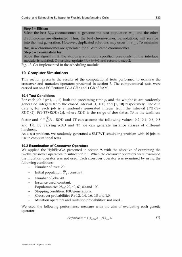
this, new chromosomes are generated for all duplicated chromosomes. Step 6 – Termination test Stops the algorithm if the stopping condition, specified previously in the interface module, is satisfied. Otherwise, update t for t:=t+1 and return to step 2.
Fig. 13. GA implemented in the scheduling module.
10. Computer Simulations
This section presents the results of the computational tests performed to examine the crossover and mutation operators presented in section 7. The computational tests were carried out on a PC Pentium IV, 3 GHz and 1 GB of RAM.
10.1 Test Conditions
For each job i (i=1, ..., n) both the processing time pi and the weight wi are randomly generated integers from the closed interval [1, 100] and [1, 10] respectively. The due date di for each job is a randomly generated integer from the interval [P(1-TF-RDD/2), P(1-TF+RDD/2)], where RDD is the range of due dates, TF is the tardiness
factor and ∑=
=n
i ipP1
. RDD and TF can assume the following values: 0.2, 0.4, 0.6, 0.8
and 1.0. By varying RDD and TF we can generate instance classes of different hardness. As a test problem, we randomly generated a SMTWT scheduling problem with 40 jobs to use in computational tests.
10.2 Examination of Crossover Operators
We applied the HybFlexGA presented in section 9, with the objective of examining the twelve crossover operators in subsection 8.1. When the crossover operators were examined the mutation operator was not used. Each crossover operator was examined by using the following conditions:
− Number of tests: 20.
− Initial population tΨ : constant.
− Number of jobs: 40.
− Instance used: constant.
− Population size Npop: 20, 40, 60, 80 and 100.
− Stopping condition: 1000 generations.
− Crossover probabilities Pc: 0.2, 0.4, 0.6, 0.8 and 1.0.
− Mutation operators and mutation probabilities: not used.
We used the following performance measure with the aim of evaluating each genetic operator:
)()( endinitial xfxfePerformanc −= , (1)
www.intechopen.com

334 Industrial Robotics - Programming, Simulation and Applications
where initialx is the best chromosome in the initial population and endx is the best
chromosome in the last population. That is, )( initialxf is the fitness average (of the 20
computational tests) of the best chromosomes in the initial population and )( endxf is the
fitness average of the best chromosomes in the end of the 1000 generations. The performance measure in (1) gives the total improvement in fitness during the execution of the genetic algorithm. We used 20 computational tests to examine each crossover operator. The average value of the performance measure in (1) was calculated for each crossover operator with each crossover probability and each population size. Table 4 shows the best average value of the performance measure obtained by each crossover operator with its best crossover probability and its best population size. This table shows the crossover operator by classification order.
Position Crossover Pc Npop Performance
1st TPC4C 1.0 100 3834.1
2nd TPC3CV2 1.0 100 3822.9
3rd TPC2CV2 1.0 100 3821.8
4th PBX 1.0 80 3805.8
5th TPC1CV2 0.8 100 3789.3
6th CX 0.8 80 3788.7
7th TPC3CV1 0.8 80 3680.2
8th TPC2CV1 1.0 80 3662.1
9th OPC2C 0.6 100 3647.8
10th OX 1.0 100 3635.4
11th TPC1CV1 1.0 100 3624.7
12th OPC1C 0.6 100 3570.5
Table 4. Classification of the crossover operators.
Fig. 14 presents the CPU time average and the fitness average along the 1000 generations. As we can see in Fig. 14 a), TPC4C, TPC3CV2 and TPC2CV2 require more CPU time than the other crossover operators. On the other hand, Fig. 14 b) shows these crossover operators present a very fast evolution at first (in the first 100 generations).
0 100 200 300 400 500 600 700 800 900 10000
100
200
300
400
500
600
700
Generation
CPU Time Average (sec.)
TPC4C, Pc=1.0, Npop=100
TPC3CV2, Pc=1.0, Npop=100
TPC2CV2, Pc=1.0, Npop=100
PBX, Pc=1.0, Npop=80
TPC1CV2, Pc=0.8, Npop=100
CX, Pc=0.8, Npop=80
100 200 300 400 500 600 700 800 900 1000
2000
2200
2400
2600
2800
3000
Generation
Average
TPC4C, Pc=1.0, Npop=100
TPC3CV2, Pc=1.0, Npop=100
TPC2CV2, Pc=1.0, Npop=100
PBX, Pc=1.0, Npop=80
TPC1CV2, Pc=0.8, Npop=100
CX, Pc=0.8, Npop=80
a) b)
Fig. 14. The six best crossover operators: a) CPU time average along the 1000 generations b) Fitness average along the 1000 generations
www.intechopen.com
Control and Scheduling Software for Flexible Manufacturing Cells 335
For the same number of generations, PBX and CX do not need as much CPU time (see Fig. 14 a)) but, these operators present a worse fitness average evolution (see Fig. 14 b)). These crossover operators obtained the best performance for Npop=80 (see Table 4) and this is one of the reasons both obtained a good CPU time average. From Fig. 14 b) we can see TPC4C is the best crossover operator along the 1000 generations, but Fig. 14 a) shows that it needed more CPU time.
10.3 Examination of Mutation Operators
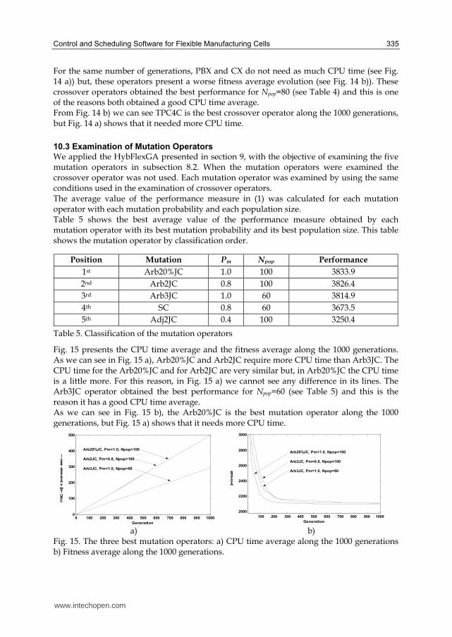
We applied the HybFlexGA presented in section 9, with the objective of examining the five mutation operators in subsection 8.2. When the mutation operators were examined the crossover operator was not used. Each mutation operator was examined by using the same conditions used in the examination of crossover operators. The average value of the performance measure in (1) was calculated for each mutation operator with each mutation probability and each population size. Table 5 shows the best average value of the performance measure obtained by each mutation operator with its best mutation probability and its best population size. This table shows the mutation operator by classification order.
Position Mutation Pm Npop Performance
1st Arb20%JC 1.0 100 3833.9
2nd Arb2JC 0.8 100 3826.4
3rd Arb3JC 1.0 60 3814.9
4th SC 0.8 60 3673.5
5th Adj2JC 0.4 100 3250.4
Table 5. Classification of the mutation operators
Fig. 15 presents the CPU time average and the fitness average along the 1000 generations. As we can see in Fig. 15 a), Arb20%JC and Arb2JC require more CPU time than Arb3JC. The CPU time for the Arb20%JC and for Arb2JC are very similar but, in Arb20%JC the CPU time is a little more. For this reason, in Fig. 15 a) we cannot see any difference in its lines. The Arb3JC operator obtained the best performance for Npop=60 (see Table 5) and this is the reason it has a good CPU time average. As we can see in Fig. 15 b), the Arb20%JC is the best mutation operator along the 1000 generations, but Fig. 15 a) shows that it needs more CPU time.
0 100 200 300 400 500 600 700 800 900 10000
100
200
300
400
500
Generation
CPU Time Average (sec.)
Arb20%JC, Pm=1.0, Npop=100
Arb2JC, Pm=0.8, Npop=100
Arb3JC, Pm=1.0, Npop=60
100 200 300 400 500 600 700 800 900 1000
2000
2200
2400
2600
2800
3000
Generation
Average
Arb20%JC, Pm=1.0, Npop=100
Arb2JC, Pm=0.8, Npop=100
Arb3JC, Pm=1.0, Npop=60
a) b)
Fig. 15. The three best mutation operators: a) CPU time average along the 1000 generations b) Fitness average along the 1000 generations.
www.intechopen.com
336 Industrial Robotics - Programming, Simulation and Applications
11. Computational Results
This section presents the computational results obtained in the single machine total weighted tardiness (SMTWT) problem. In the SMTWT n jobs have to be sequentially processed on a single machine. Each job i has an associated processing time pi, a weight wi, and an associated due date di associated, and the job becomes available for processing at time zero. The tardiness of a job i is defined as Ti=max{0, Ci-di}, where Ci is the completion time of job i in the current job sequence. The objective is to find a
job sequence which minimizes the sum of the weighted tardiness given by ∑=
n
i
ii Tw1
. .
For arbitrary positive weights, the SMTWT problem is strongly NP-hard (Lenstra et al., 1977). Because the SMTWT problem is NP-hard, optimal algorithms for this problem would require a computational time that increases exponentially with the problem size (Morton & David, 1993), (Baker, 1974), (Lawer, 1977), (Abdul-Razaq et al., 1990) and (Potts & Wassenhove, 1991). Several algorithms have been proposed to solve this, for example: branch and bound algorithms (Shwimer, 1972), (Rinnooy et al., 1975), (Potts & Wassenhove, 1985) and dynamic programming algorithms (Schrage & Baker, 1978), have been proposed to generate exact solutions, i.e., solutions that are guaranteed to be optimal solutions. But, the branch and bound algorithms are limited by computational times and the dynamic programming algorithms are limited by computer storage requirements, especially when the number of jobs is more than 50. Thereafter, the SMTWT problem was extensively studied by heuristics. These heuristics generate good or even optimal solutions, but do not guarantee optimality. In recent years, several heuristics, such as Simulated Annealing, Tabu Search, Genetic Algorithms and Ant Colony (Huegler & Vasko, 1997), (Crauwels et al., 1998), and (Morton & David, 1993), have been proposed to solve the SMTWT problem. We going to present, in this section, the computational results obtained with 40, 50 and 100 jobs, using Genetic Algorithms. From the OR-Library (http#3), we randomly selected some instances of SMTWT problems with 40, 50 and 100 jobs. We used 20 computational tests for each instance of SMTWT problem. We used the six best crossover operators (see Table 4) and the best mutation operator (see Table 5) in the HybFlexGA. Each instance of SMTWT problem was examined by using the following conditions:
− Number of tests: 20.
− Initial population tΨ : randomly generated.
− Number of jobs: 40, 50 and 100.
− Instance used: from the OR-Library (http#3).
− Population size Npop: 80 and 100 (see Table 4 and Table 5).
− Stopping condition: 1000 generations for the instances with 40 and 50 jobs or the optimal solution, and 5000 generations for the instances with 100 jobs or the optimal solution.
− Crossover operators: the six best crossover operators in Table 4.
− Crossover probabilities Pc: 0.8 and 1.0 (see Table 4).
− Mutation operators: the best mutation operator in Table 5.
− Mutation probabilities Pm: 1.0 (see Table 5).
www.intechopen.com

Control and Scheduling Software for Flexible Manufacturing Cells 337
Instance 40A 40B 40C 50A 50B 50C 100A 100B 100C
Optimal solution 6575 1225 6324 2134 22 2583 5988 8 4267
Tests with optimal solution
16 20 19 20 20 15 16 20 19
CPU time average (sec.)
362.4 190.0 319.7 88.3 45.5 214.1 2405.1 523.9 3213.5
TPC4C +
Arb20%JC
Generations average 593 284 475 107 54 256 1611 323 1971
Tests with optimal solution
13 15 15 18 20 12 15 20 15
CPU time average (sec.)
382.9 231.3 260.5 112.3 50.4 207.9 3851.0 1012.4 4453.7
TPC3CV2 +
Arb20%JC Generations average 725 402 448 158 70 290 3042 727 3181
Tests with optimal solution
8 16 15 17 20 12 9 20 5
CPU time average (sec.) 369.1 216.8 305.8 146.2 92.0 157.8 3921.3 1339.8 4036.2
TPC2CV2 +
Arb20%JC
Generations average 380 449 627 246 152 263 3685 1142 3423
Tests with optimal solution
0 8 1 18 20 10 1 20 3
CPU time average (sec.)
--- 236.1 312.0 144.6 86.3 151.6 2067.0 1413.6 3237.7
PBX +
Arb20%JC
Generations average --- 747 976 371 218 385 2957 1828 4182
Tests with optimal solution
0 3 2 13 20 5 1 19 2
CPU time average (sec.)
--- 230.0 363.5 224.7 118.2 180.0 4104.0 2190.7 3847.0
TPC1CV2 +
Arb20%JC Generations average --- 609 956 487 252 385 4948 2405 4192
Tests with optimal solution
0 4 4 17 20 11 3 20 5
CPU time average (sec.)
--- 165.3 270.5 107.8 51.0 140.0 2594.0 736.4 3224.2
CX +
Arb20%JC
Generations average --- 551 892 292 136 375 3912 1011 4390
Table 6. Computational results obtained for the SMTWT problems with 40, 50 and 100 jobs.
Table 6 shows the computational results obtained for the SMTWT problems with 40, 50 and 100 jobs. In this table, we have the number of tests with optimal solution, the CPU time average (in seconds) and the generations average for each instance problem. For example, we chose the TPC4C with Pc=1.0, Arb20%JC with Pm=1.0 and instance 40A (SMTWT problem with 40 jobs, from the OR-Library (http#3)) in the HybFlexGA. We did 20 computational tests for this instance. In these tests we obtained the optimal solutions in 16 tests. In these 16 tests, the CPU time average was 362.4 seconds and the generation average was 593. As we can see in Table 6, we obtained good results with the TPC4C+Arb20%JC, TPC3CV2+Arb20%JC and TPC2CV2+Arb20%JC combination, for all the instances with 40, 50 and 100 jobs. But, as we can see in this table, the best results are obtained for the TPC4C+Arb20%JC combination. When we used the TPC4C+Arb20%JC combination, the HybFlexGA is very efficient. For example, in the three instances with 40 jobs (see Table 6 – 40A, 40B and 40C) the HybFlexGA found 20 tests with optimal solution in one instance (40B), 19 tests with optimal solutions in one instance (40C) and 16 tests with optimal solutions in one instance (40A).
www.intechopen.com

338 Industrial Robotics - Programming, Simulation and Applications
In subsection 10.2 and 10.3, we demonstrated that TPC4C and Arb20%JC need more CPU time (for the same generations) than the other genetic operators. But, we also demonstrated that TPC4C and Arb20%JC need fewer generations to find good solutions, probably the optimal solutions. The computational results obtained in Table 6 show the HybFlexGA with the TPC4C+Arb20%JC combination requires less CPU time than the one with the other combinations. For example, in the 50B instance the HybFlexGA always found the optimal solution for all combinations (e.g., TPC3CV2+Arb20%JC, TPC2CV2+Arb20%JC, and so on). For this instance, as we can see in Table 6, the combination that needs less CPU time average was the TPC4C+Arb20%JC (45.5 seconds). All the other combinations need more CPU time average.
12. Conclusion
Robust control software is a necessity for an automated FMS and FMC, and plays an important role in the attainable flexibility. Often FMS and FMC are built with very flexible machines (robots, CNC machines, ASRS, etc) but the available control software is unable to exploit the flexibility of adding new machines, parts, changing control algorithms, etc. The present robot control and CNC machines control systems are closed and with deficient software interfaces. Nowadays, the software is typically custom written, very expensive, difficult to modify, and often the main source of inflexibility in FMS. We have developed a collection of software tools: “winRS232ROBOTcontrol”, “winEthernetROBOTcontrol”, “winMILLcontrol”, “winTURNcontrol” and USB software. These software tools allow the development of industrial applications of monitoring and controlling robotic networks and CNC machines inserted in FMS or FMC. All the software developed has operation potentialities in Ethernet. The basic idea is to define for any specific equipment a library of functions that in each moment define the basic functionality of that equipment for remote use. In this chapter we also propose a new concept of genetic operators for scheduling problems. We developed a software tool called HybFlexGA, to examine the performance of various crossover and mutation operators by computing simulations on job scheduling problems. The HybFlexGA obtained good computational results in the instances of SMTWT problems with 40, 50 and 100 jobs (see Table 6). As we demonstrated, the HybFlexGA is very efficient with the TPC4C+Arb20%JC combination. With this combination, the HybFlexGA always found more optimal solutions than with the other combinations: TPC3CV2+Arb20%JC, TPC2CV2+Arb20%JC, and so on. When we used this combination (TPC4C+Arb20%JC) in the HybFlexGA, the genetic algorithm required fewer generations and less CPU time to find the optimal solutions. These results show the good performance and efficiency of the HybFlexGA with the TPC4C and Arb20%JC genetic operators. Application of the HybFlexGA, with these same genetic operator combinations, in other scheduling problems (e.g. job-shop and flow-shop) is left for future work.
13. References
Abdul-Razaq, T.; Potts C. & Wassenhove L. (1990). A survey for the Single-Machine Scheduling Total WT Scheduling Problem. Discrete Applied Mathematics, No 26, (1990), pp. 235–253.
Baker, R. (1974). Introduction to Sequencing and Scheduling, Wiley, New York.
www.intechopen.com
Control and Scheduling Software for Flexible Manufacturing Cells 339
Crauwels H.; Potts C. & Wassenhove L. (1998). Local search heuristics for the single
machine total weighted tardiness scheduling problem. INFORMS Journal on
Computing, Vol. 10, No 3, (1998), pp. 341–350.
Ferrolho A.; Crisóstomo M. & Lima M. (2005). Intelligent Control Software for Industrial
CNC Machines, Proceedings of the IEEE 9th International Conference on Intelligent
Engineering Systems, Cruising on Mediterranean Sea, September 16-19, 2005, in CD-
ROM.
Ferrolho A. & Crisóstomo M. (2005-a). Scheduling and Control of Flexible Manufacturing
Cells Using Genetic Algorithms. WSEAS Transactions on Computers, Vol. 4, 2005, pp.
502–510.
Ferrolho A. & Crisóstomo M. (2005-b). Flexible Manufacturing Cell: Development,
Coordination, Integration and Control, in Proceedings of the IEEE 5th Int.
Conference on Control and Automation, pp. 1050-1055, Hungary, June 26-29, 2005,
in CD-ROM.
Ferrolho A. & Crisóstomo M. (2005-c). Genetic Algorithms for Solving Scheduling Problems
in Flexible Manufacturing Cells, in Proceedings of the 4th WSEAS International
Conference on Electronics, Signal Processing and Control (ESPOCO2005), Brazil, April
25-27, 2005, in CD-ROM.
Ferrolho A. & Crisóstomo M. (2005-d). Genetic Algorithms: concepts, techniques and
applications. WSEAS Transactions on Advances in Engineering Education, Vol. 2, 2005,
pp. 12–19.
French S. (1982). Sequencing and Scheduling: An Introduction to the Mathematics of the Job-Shop,
John Wiley & Sons, New York.
Goldberg D. (1989). Genetic Algorithms in Search, Optimization and Machine Learning,
Addison-Wesley.
Hadj-Alouane N.; Chaar J.; Naylor A. & Volz R. (1988). Material handling systems as
software components: An implementation. Tech. Paper, Center for Res. on Integrated
Manufacturing. The Univ. Michigan, May 1988.
Huegler P. & Vasko F. (1997). A performance comparison of heuristics for the total weighted
tardiness problem. Computers & Industrial Engineering, Vol. 32, No 4, (1997), pp.
753–767.
Joshi S.; R. A. Wysk & E. G. Mettala (1991). Automatic Generation of Control System
Software for Flexible Manufacturing Systems. IEEE Trans. on Robotics and
Automation, Vol. 7, No. 6, (December 1991) pp. 283–291.
Joshi, S.; J. S. Smith; R. A. Wysk; B. Peters & C. Pegden (1995). Rapid-CIM: An approach to
rapid development of control software for FMS control. 27th CIRP International
Seminar on Manufacturing Systems, Ann Arbor, MI, 1995.
Kusiak A., (1986). Modelling and Design of Flexible Manufacturing Systems, Elsevier Science
Publishers.
Lawer, E. (1977). A pseudopolinomial algorithm for Sequencing Jobs to Minimize Total
Tardiness. Annals of Discrete Mathematics, (1977), pp. 331–342.
Lenstra J.; Kinnooy Kan H. & Brucker P. (1977). Complexity of machine scheduling
problems. Annals of Discrete Mathematics, Vol. 1 (1977), pp. 343–362.
Maimon O. & Fisher E. (1988). An object-based representation method for a manufacturing
cell controller. Artificial Intelligence in Engineering, Vol. 3, No. 1.
Morton, E. & David W. (1993). Heuristic Scheduling Systems, John Wiley & Sons.
www.intechopen.com

340 Industrial Robotics - Programming, Simulation and Applications
Murata T. & Ishibuchi H. (1994). Performance Evaluation of Genetic Algorithms for Flowshop Scheduling Problems, Proceedings of the 1st IEEE Int. Conference on Evolutionary Computation, pp. 812–817, Orlando, USA.
Oliver J.; Smith D. & Holland J. (1987). A study of permutation crossover operators on the traveling salesman problem, Proceedings of the Second ICGA , pp. 224–230.
Potts C. & Wassenhove L.(1985). A branch and bound algorithm for the total weighted tardiness problems. Operations research, Vol. 33, No 2, (1985), pp. 363–377.
Potts, C. & Wassenhove L. (1991). Single Machine Tardiness Sequencing Heuristics. IIE Transactions, Vol. 23, No 4, (1991), pp. 346–354.
Rembold U.; Nnaji B. & Storr A. (1993). Computer Integrated Manufacturing and Engineering, Addison-Wesley.
Rinnooy H.; Lageweg B. & Lenstra J. (1975). Minimizing total costs in one-machine scheduling. Operations research, Vol. 23, No 5, (1975), pp. 908–927.
Sanjay B. Joshi; Erik G. Mettala; Jeffrey S. Smith & Richard A. Wysk (1995). Formal Models for Control of Flexible Manufacturing Cells: Physical and System Model. IEEE Trans. on Robotics and Automation, Vol. 11, No. 4, (August 1995) pp. 558–570.
Schrage L. & Baker K. (1978). Dynamic programming solution of sequencing problem with precedence constraints. Operations research, Vol. 26, (1978), pp. 444–449.
Shwimer J. (1972). On the n-job, one-machine, sequence-independent scheduling problem with tardiness penalties: a branch-bound solution. Management Science, Vol. 18, No 6, (1972), pp. 301–313.
Syswerda G. (1991). Scheduling optimization using genetic algorithms. L. Davis (Ed.) Handbook of Genetic Algorithms, Van Nostrand Reinhold, New York, pp. 332–349.
Waldner JB., (1992). CIM, Principles of Computer Integrated Manufacturing, John Wiley & Sons.
Sites WWW http#1 - Rapid Prototyping and Development of FMS Control Software for Computer
Integrated Manufacturing. Available: http://tamcam.tamu.edu/rapidcim/ rc.htm
http#2 - RapidCIM. Available: http://www.engr.psu.edu/cim/ http#3 - http://people.brunel.ac.uk/~mastjjb/jeb/orlib/wtinfo.html
www.intechopen.com

Industrial Robotics: Programming, Simulation and ApplicationsEdited by Low Kin Huat
ISBN 3-86611-286-6Hard cover, 702 pagesPublisher Pro Literatur Verlag, Germany / ARS, Austria Published online 01, December, 2006Published in print edition December, 2006
InTech EuropeUniversity Campus STeP Ri Slavka Krautzeka 83/A 51000 Rijeka, Croatia Phone: +385 (51) 770 447 Fax: +385 (51) 686 166www.intechopen.com
InTech ChinaUnit 405, Office Block, Hotel Equatorial Shanghai No.65, Yan An Road (West), Shanghai, 200040, China
Phone: +86-21-62489820 Fax: +86-21-62489821
This book covers a wide range of topics relating to advanced industrial robotics, sensors and automationtechnologies. Although being highly technical and complex in nature, the papers presented in this bookrepresent some of the latest cutting edge technologies and advancements in industrial robotics technology.This book covers topics such as networking, properties of manipulators, forward and inverse robot armkinematics, motion path-planning, machine vision and many other practical topics too numerous to list here.The authors and editor of this book wish to inspire people, especially young ones, to get involved with roboticand mechatronic engineering technology and to develop new and exciting practical applications, perhaps usingthe ideas and concepts presented herein.
How to referenceIn order to correctly reference this scholarly work, feel free to copy and paste the following:
Antonio Ferrolho and Manuel Crisostomo (2006). Control and Scheduling Software for Flexible ManufacturingCells, Industrial Robotics: Programming, Simulation and Applications, Low Kin Huat (Ed.), ISBN: 3-86611-286-6, InTech, Available from:http://www.intechopen.com/books/industrial_robotics_programming_simulation_and_applications/control_and_scheduling_software_for_flexible_manufacturing_cells
Top Related