


Languages
Pages
Legal


Contracts and Capacity Investment in Supply Chains
Andrew M. DavisSamuel Curtis Johnson Graduate School of Management, Cornell University, Ithaca, NY 14853, [email protected],
Stephen G. LeiderRoss School of Management, University of Michigan, Ann Arbor, MI 48109, [email protected],
Suppliers are often reluctant to invest in capacity if they believe that they will be unable to recover their
investment costs in subsequent transactions with buyers. In theory, a number of different contracts can solve
this issue and induce first-best investment levels by the supplier. In this study, we investigate the performance
of these contracts in a two-tier supply chain. We develop an experimental design where retailers and suppliers
bargain over contract terms, and have the ability to make multiple back-and-forth offers, while also providing
feedback on the offers they receive. One key result from our study is that an option contract and a service-
level agreement are best at increasing first-best investment levels and overall supply chain profits. However,
these same contracts also generate the largest inequity in expected profits between the two parties. We find
that both of these results are driven by the bargaining tendencies of retailers and suppliers, which we refer
to as “superficial fairness.” In particular, (1) retailers and suppliers place more emphasis on negotiating the
wholesale price, while partially overlooking any secondary parameter, and (2) they make concessions over
time, such that final wholesale prices end up roughly halfway between the retailer’s selling price and the
supplier’s production cost. We show that this bargaining behavior contributes to higher investment levels in
the option contract and service-level agreement, but also highly inequitable payoffs.
1. Introduction
Firms often face the challenge of ensuring that their suppliers develop and maintain sufficient
production capacity. A classic example of this involves General Motors (GM) purchasing metal
car bodies from its supplier, Fisher Body (Klein et al. 1978, Coase 2006, Klein 2007). As demand
increased, GM wanted Fisher to continue expanding its plants to increase capacity. However, in an
example such as this, a supplier like Fisher Body may be reluctant to make investments, such as
developing capacity, if they believe that their future profits will be insufficient, either due to low
bargaining power or ex post opportunism. As a result, they may invest in less capacity than what
would be jointly optimal (first best). Further, Cachon and Lariviere (2001), in a related capacity
investment setting with forecast sharing, highlight a number of examples where suppliers are left
without returns from their capacity investments, and suggest that “suppliers may be wise to avoid
spending heavily to serve assemblers”(Cachon and Lariviere 2001, pp. 630).
To increase supplier capacity investment levels, theoretical research has proposed a number
of solutions. Vertical integration aligns the firms’ incentives, but can involve substantial costs
1
2 Davis and Leider: Contracts and Capacity Investment in Supply Chains
and presents additional risks and challenges (Stuckey and White 1993). Long run buyer-supplier
relationships can also promote investment. However, the scope of many capacity investments, and
the likelihood that market characteristics will change, can make long run relationships difficult
to maintain. Formal contracts can provide direct or indirect incentives to invest, and have been
highlighted in the operations management literature as a leading solution (e.g. Tomlin 2003, Ozer
and Wei 2006, Plambeck and Taylor 2007, Taylor and Plambeck 2007). In this study, we focus on
contractual solutions to capacity investment problems. Specifically, we conduct a series of controlled
human-subject experiments which determine whether different contractual solutions can increase
supplier capacity investment levels and supply chain profits, when allowing human decision makers
to bargain over contract parameters and make capacity investment decisions.
While there have been a number of papers analyzing capacity investment problems from a the-
oretical standpoint, only a few experimental studies exist on the topic (e.g. Hoppe and Schmitz
2011). Many of these assume settings with deterministic demand and simplified bargaining. In our
study, we incorporate a two-stage supply chain where demand is randomly determined, and imple-
ment a unique structured bargaining protocol which allows both a retailer and supplier to make
multiple, back-and-forth offers over contract parameters. Additionally, in our bargaining setting,
subjects can send limited feedback, detailing whether they feel a particular contract parameter
is too high or too low. Through this bargaining protocol we are able to not only mimic a more
realistic environment, but also observe how offers evolve over time and the types of feedback sent.
Using this experimental design with human decision makers we evaluate the problem of supplier
capacity investment, with the aim of answering the following research questions: (1) How do alter-
native contracts, many of which are equivalent in theory, perform at increasing first-best investment
rates and overall supply chain profits? (2) Of those contracts that are effective at inducing first-best
investment rates, how are supply chain profits distributed between the retailer and supplier? and
(3) What is the behavioral driver which generates any observed differences across contracts?
We begin by theoretically investigating several contractual solutions to the capacity investment
problem under two-point demand, and show that, in theory, many of the contracts (a price premium
for higher quantities, a minimum quantity commitment, an option fee for investing in capacity,
and a bonus for satisfying demand) allow for various combinations of contract parameters that can
generate first-best capacity investment decisions for suppliers, and also equalize expected profits
between the retailer and supplier. We then conduct a series of experiments directly testing these
theoretical predictions, and find that the contracts perform quite differently than the normative
benchmarks. In particular, our first main experimental result is that the option contract, where

Davis and Leider: Contracts and Capacity Investment in Supply Chains 3
the supplier receives a fixed option fee from the retailer that is forfeit whenever the supplier fails
to invest in capacity, and service-level agreement, where the retailer awards the supplier a bonus
anytime she can satisfy all of demand, both perform substantially better than the other contracts at
increasing supplier investment, and thus generating higher expected supply chain profits. However,
another key result is that, these same contracts, while best at inducing higher levels of first-best
investment, are also tied to the most inequitable payoffs. More specifically, we observe that as
certain contracts increase overall supply chain profits, these gains heavily favor the supplier.
The bargaining data from our study suggest that there are two primary reasons for these exper-
imental results, which we collectively refer to as “superficial fairness.” In particular, (1) when
retailers and suppliers bargain over multiple contract parameters, both parties, across all contracts,
devote more effort towards negotiating the wholesale price, while largely overlooking the secondary
parameter (such as a secondary wholesale price, quantity commitment, option fee, or bonus), and
(2) subjects make concessions while bargaining, that is, they first make an initial wholesale price
offer that greatly favors themselves, and then each make concessions until the final wholesale price
is roughly in the middle of the supplier’s production cost per unit and the retailer’s revenue per
unit. We show that these behavioral tendencies can account not only for the favorable performance
of the option contract and service-level agreement, in terms of overall investment rates and supply
chain profits, but also the observed distribution of expected profits between the two parties.
In an effort to determine whether the results from our main study are sensitive to our experi-
mental setting, we conduct two additional robustness studies. The first considers a slightly altered
demand setting where superficial fairness, if present, should lead to increased investment rates
(which we do observe). The second robustness study incorporates a slightly richer environment,
by assuming that demand is continuous. In both of these robustness checks, we find support for
each of our main experimental results. For instance, we find that the option contract continues to
perform best at increasing supply chain profits, but also, tends to significantly favor the supplier.
Furthermore, in both studies, we continue to find evidence of superficial fairness.
In Section 2 we summarize the relevant literature. In Section 3, we outline the theoretical details
of our contractual solutions. In Section 4, we summarize the experimental design, and present our
results in Section 5. We then detail two separate robustness studies in Section 6, and then conclude
with a discussion of our results, managerial implications, and future research in Section 7.
2. Related Literature
The general problem of under-investment over a relation-specific investment, when the returns
are expropriable by another party, has been extensively studied in the economics literature. The

4 Davis and Leider: Contracts and Capacity Investment in Supply Chains
most prominent theoretical solutions to this problem include vertical integration, contracting, and
repeated interaction (e.g. Klein et al. 1978, Williamson 1979, Grossman and Hart 1986, Hart
and Moore 1990, Chung 1991, Klein and Leffler 1981, Baker et al. 2002). From an experimental
economics standpoint, Sloof et al. (2004), Ellingsen and Johannesson (2004) and Sloof (2008)
test whether investment decisions respond to the structure of the situation as theory predicts in
certain settings. Most relevant to our study are experimental economics works which test the role
of contracts and organizational form as solutions to capacity investment problems. In particular,
Hoppe and Schmitz (2011) study whether contracts can improve decisions when renegotiation is
possible. Fehr et al. (2008) and Dufwenberg et al. (2013) examine how the allocation of control
rights affects results. In general, a majority of these studies focus on settings with deterministic
outcomes from decisions, and one-shot ultimatum offers, whereas our work attempts to extend this
literature by incorporating random demand, and allowing for dynamic structured bargaining.
In terms of bargaining research, the theoretical literature is quite rich, including process-free
bargaining solutions (such as the Nash Bargaining Solution, Nash 1950), game-theoretic analyses of
sequential bargaining games (Rubenstein 1982), and many other approaches (see Muthoo 1999 for a
comprehensive summary). From an experimental perspective, studies exploring bargaining typically
apply one of two extreme structures; ultimatum one-shot take-it-or-leave it offers or complete free
form negotiation. The former is useful in that theoretical benchmarks are more easily derived and
tested (e.g. Davis et al. 2014), however, an ultimatum environment may stray from a back-and-
forth negotiation where both players have similar bargaining power. On the other hand, complete
free form negotiation is attractive in capturing a more realistic bargaining process (e.g. Leider and
Lovejoy 2016), however, there is a risk of losing control in the laboratory (i.e. participants revealing
personal information or making appeals to context not present in the experiment). In our study, we
develop and implement a bargaining protocol that lies in between these two extreme structures. In
particular, our study allows both players to make multiple offers, and also permits players to send
limited feedback about offers received. Thus, we attempt take a step towards representing a more
natural bargaining process, while still having the ability to observe offers, including rejected ones,
and the types of feedback sent. Both ultimatum and free-form negotiation experiments reliably
show that fairness is a major concern (e.g. Guth et al. 1982, Guth and Tietz 1990, Leider and
Lovejoy 2016), and therefore we expect fairness to play an important role in our setting.
Our paper also draws on the extensive literature in economics and psychology on biases in
bargaining (see Bazerman and Neale 1994 and Bazerman et al. 2000 for excellent surveys of the
psychology literature on negotiation biases, and Roth 1995 and Camerer 2003 Ch. 4 for surveys

Davis and Leider: Contracts and Capacity Investment in Supply Chains 5
of the experimental economics literature on bargaining). One prominent bias that is particularly
relevant in our setting is the “fixed-pie bias” - i.e. the (incorrect) belief by negotiators that they
should primarily focus on bargaining over how to divide a fixed surplus, and a failure to recog-
nize opportunities for joint gain (Thompson and Hastie 1990, Thompson and DeHarpport 1990,
Fukuno and Ohbuchi 1997). Thompson and Hastie (1990) show that one source of the bias is that
negotiators typically enter a bargaining setting presuming that the other party’s preferences are
diametrically opposed to their own. Thompson and DeHarpport (1990) show that this is primarily
a judgement problem, as accurate feedback on the other party’s true interests can significantly
mitigate the bias. Thompson and Hrebec (1996) show that joint agreements in an interdependent
decision-making setting similarly fail to recognize opportunities for mutual gain.
A second prominent bias is that negotiators often have subjective and self-serving perceptions
of what outcomes are fair (Thompson and Loewenstein 1992, Babcock and Loewenstein 1997).
Bargaining, therefore, does not always converge to equalizing (expected) outcomes between parties
in the way that more traditional social preference models of fairness would suggest (Fehr and
Schmidt 1999, Bolton and Ockenfels 2000). For example, in a series of binary lottery bargaining
experiments (Roth and Malouf 1979, Roth et al. 1981, Roth and Malouf 1982), Roth, Malouf and
Murnighan (1981) show that when the negotiating subjects have asymmetric payoffs for winning
the lottery, they will tend to disagree over whether the “fair” outcome involves giving each party
an equal number of tickets (favored by the subject with the larger payoff for winning) or an equal
expected value (favored by the subject with the lower payoff for winning).
Finally, negotiators often address a multi-issue negotiation by addressing each issue separately
and sequentially (Mannix et al. 1989, Weingart et al. 1993). This can lead negotiators to overem-
phasize certain issues, and to fail to appreciate how multiple issues interact to generate joint gains.
Together, these biases suggest several things for our setting. First, during the negotiations subjects
are likely to focus on the contractual terms separately, rather than on how they work together to
affect outcomes. Second, they are likely to focus on claiming value, rather than finding ways to
increase joint surplus (especially since the retail price is fixed, so the only way to increase the sur-
plus is to affect the capacity decision) or equalize expected payoffs. We might then expect subjects
to primarily focus on bargaining over the wholesale price, as it is a salient contract term that (on
the surface) divides the fixed per-unit revenue.
If indeed subjects during bargaining fail to appreciate how the contractual terms work together
to provide incentives, the structure and directness of the incentives under different contractual
forms may be particularly important. Both theoretical (Kerr 1975, Holmstrom and Milgrom 1991,

6 Davis and Leider: Contracts and Capacity Investment in Supply Chains
Baker 1992) and experimental (Philipson and Lawless 1997, Fehr and Schmidt 2004, Scheele et al.
2014, Al-Ubaydli et al. 2015) evidence suggests that incentives that are partial, indirect or mis-
aligned with the ultimate goal will likely perform worse. This intuition is often called the “folly of
rewarding A, while hoping for B” (Kerr 1975). In our setting the option contract provides the most
direct incentives towards capacity investment, while the incentives of other coordinating contracts
(quantity premium and quantity commitment) are more indirect. Hence, if negotiation biases cause
subjects not to fine-tune contract parameters, these results would suggest that the contract with
the most direct incentives, the option contract, will achieve the best performance.
From an operations management standpoint, there are a number of theoretical studies on capac-
ity investment decisions in various settings. The most relevant are those which evaluate how con-
tracts can induce a supplier to invest in capacity for a retailer. For example, Cachon and Lariviere
(2001) investigate an asymmetric information setting where a manufacturer can share its forecast
demand information with a sole-source supplier, and the supplier makes a decision about how much
capacity to install. Tomlin (2003) extends Cachon and Lariviere (2001), in that both a manufac-
turer and supplier invest in capacity. Ozer and Wei (2006) also extend Cachon and Lariviere (2001)
by examining how a supplier can screen buyers, under asymmetric information, by offering a menu
of contracts. Plambeck and Taylor (2005) evaluate a scenario with original equipment manufactur-
ers selling production to contract manufacturers, and identify how pooling and bargaining power
affect investments in innovation and capacity. Taylor and Plambeck (2007), in a classic capacity
investment decision setting, derive optimal price, and price with quantity, contracts and explore
which contract is best under different production and capacity costs. There has also been some
work in operations that considers how human decision makers set various contract terms, such as
Becker-Peth and Thonemann (2016). We believe our work is unique to this rich literature by tak-
ing a behavioral standpoint, and identifying contractual solutions to capacity investment problems
with human decision makers interacting under a more natural bargaining setting.
3. Theory
One common solution to the capacity investment problem is to allow the parties to negotiate a
contract prior to any supplier investment decision. In this section, we present a theoretical review
of five contracts (wholesale price, quantity premium, quantity commitment, option, and a service-
level agreement), which are all used in practice (Lovejoy 2010, Plambeck and Taylor 2007, Oblicore
2007), and can induce the supplier to invest in capacity through different mechanisms. For example,
the quantity premium contract can lead to first-best investment through the use of multiple prices,

Davis and Leider: Contracts and Capacity Investment in Supply Chains 7
whereas the quantity commitment contract makes investment attractive through a minimum order
quantity by retailers.
For all contracts, assume demand follows a two-point distribution, with high demand D, low
demand d, and difference in demand δ= (D−d). High demand D occurs with probability p, and low
demand d occurs with probability (1−p). The supplier (S) manufactures products instantaneously,
begins with sufficient capacity to make d units, and can incur a fixed cost of K to increase capacity
to D units. We assume that the supplier’s capacity is only useful to satisfy demand for the retailer’s
(R) product, that is, capacity is relationship-specific to the retailer.
There is full information for both parties about the model parameters. Let r represent the
retailer’s revenue per unit, and c= 0 denote the supplier’s marginal cost of production per unit. The
retailer and supplier agree ex ante, before the supplier’s investment decision, to buy and sell units
at a wholesale price w, 0≤w≤ r, plus any additional contract terms. We assume that investment
in capacity is beneficial for the overall supply chain K ≤ rpδ.
Let πji (x) denote the expected profit function of party i, i ∈ {R,S}, in contract j, j ∈
{WP,QP,QC,OP,SL}, where x is the supplier’s investment decision, x∈ {Yes,No}. We will refer
to any set of contract terms where it is expected-profit maximizing for the supplier to invest in
capacity as an incentive compatible contract. Also, because renegotiation is not a focus of our study,
we assume that renegotiation is not possible, and hence incentive compatibility depends on the
initial terms of the contract, however, we discuss renegotiation-proofness in an online Appendix.
Because fairness is likely to be a concern during bargaining, we will discuss for each contract
whether fairness and incentive compatibility is jointly possible. First, we will identify the parame-
ters that both satisfy incentive compatibility and allow for equal expected profits. Second, since the
bargaining literature suggests that the wholesale price is likely to be salient and that negotiators
may have biased notions of fairness, we will specifically note what is possible when w= r2, i.e. the
wholesale price is at the midpoint between revenue and marginal cost. Table 1 in the next section
will show the specific contractual terms required given the parameters used in the experiment.
3.1 Wholesale Price Contract
Under a wholesale price (WP ) contract, the retailer and supplier agree to buy and sell units at
wholesale price w, where the expected profit functions are:
πWPR (x) =
{(r−w)d if x= No,
(r−w)(d+ pδ) if x= Yes,πWP
S (x) =
{wd if x= No,
w(d+ pδ)−K if x= Yes.

8 Davis and Leider: Contracts and Capacity Investment in Supply Chains
The WP contract is incentive compatible for the supplier if w ≥ Kpδ
. However, note that this is
equivalent to wr≥ K
rpδ, implying that as K → rpδ, then w→ r, leading to investment but requir-
ing unequal profit shares between the two parties. Equalizing expected profits further requires
that wr
= 12
+ K2r(d+pδ)
. To jointly have incentive compatibility and equal expected profits requires
rpδ≥(2d+pδd+pδ
)K, i.e. the surplus increase from the investment has to be large relative to the cost of
the investment and the amount of demand that can be covered without the investment. Addition-
ally, note that with w = r2
for incentive compatibility one would need Krpδ≤ 1
2, again requiring an
inexpensive investment. Equalizing expected profits is not possible with w = r2. Our main experi-
ment will use parameters such that K is not large enough to satisfy the conditions for equal profits
or the conditions for incentive compatibility with w = r2, however we will conduct an additional
experiment as a robustness check that uses different parameters that satisfy both conditions.
3.2 Quantity Premium Contract
A quantity premium (QP ) contract states that the retailer and supplier agree to buy and sell units
at wholesale price w1, 0≤w1 ≤ r, for the first d units, and wholesale price w2, 0≤w2 ≤ r, for any
units sold above d. In this contract the expected profit functions are as follows:
πQPR (x) =
{(r−w1)d if x= No,
(r−w1)d+ (r−w2)pδ if x= Yes,πQP
S (x) =
{w1d if x= No,
w1d+w2pδ−K if x= Yes.
The QP contract is incentive compatible when w2 ≥ Kpδ
= w2. In addition, there are a range of
QP contracts that are both incentive compatible and generate equal expected profits. In order for
this to be true, w2 = (r−2w1)d+rpδ+K
2pδ, must hold. Additionally, we must have w2 ≥ w2 (for incentive
compatibility), as well as r ≥ w2. Therefore the following two conditions are required on w1: (1)
w2 ≥ w2, if w1 ≤ r(d+pδ)−K2d
, and (2) r ≥ w2, if w1 ≥ r(d−pδ)+K2d
. Thus, a QP contract is incentive
compatible and equalizes expected profits when the following two conditions are satisfied:{w2 =
(r− 2w1)d+ rpδ+K
2pδ,r(d− pδ) +K
2d≤w1 ≤
r(d+ pδ)−K2d
}.
For w1 = r2, the incentive compatibility conditions are the same. Incentive compatibility and
equal expected profits can be jointly achieved with w2 = rpδ+K2pδ
.
3.3 Quantity Commitment Contract
Under a quantity commitment (QC) contract the retailer and supplier agree to buy and sell units
at a wholesale price of w, with a commitment that the retailer buy at least q units, d ≤ q ≤D,
regardless of demand. If the supplier does not invest, and is therefore unable to deliver q units,

Davis and Leider: Contracts and Capacity Investment in Supply Chains 9
then the retailer is released from the commitment and is free to order any amount. In the QC
contract the expected profit functions are given by:
πQCR (x) =
{(r−w)d if x= No,
(1− p)(rd−wq) + p(r−w)D if x= Yes,πQC
S (x) =
{wd if x= No,
w(q+ p(D− q))−K if x= Yes.
The QC contract is incentive compatible when q ≥ w(d−pD)+K
w(1−p) = q. As with the QP contract, in
the QC contract, there are a range of possible contracts that are incentive compatible and equalize
expected profits. To ensure this, q = (r−2w)pD+r(1−p)d+K2w(1−p) , must hold. Additionally, we must have
q≥ q, as well as d≤ q≤D, leading to three conditions on w: (1) q≥ q, if w≤ r(d+pδ)−K2d
, (2) q≥ d,
if w≤ r(d+pδ)+K
2(d+pδ), and (3) D≥ q, if w≥ r(d+pδ)+K
2D. Therefore a QC contract is incentive compatible
and equalizes expected profits between the two parties when the following conditions are satisfied:{q=
(r− 2w)pD+ r(1− p)d+K
2w(1− p),r(d+ pδ) +K
2D≤w≤min
{r(d+ pδ)−K
2d,r(d+ pδ) +K
2(d+ pδ)
}}.
For w= r2
the incentive compatibility condition becomes q≥ r(d−pD)+2K
r(1−p) . Equal expected profits
requires q= r(1−p)d+Kr(1−p) , which also satisfies incentive compatibility.
3.4 Option Contract
In the option (OP ) contract, the retailer and supplier agree to buy and sell units at a wholesale
price of w, and the retailer pays a lump sum option fee po to the supplier. If the supplier does not
invest, he will be unable to execute the terms of the contract (i.e. unable to deliver all units the
buyer has an option for), and forfeits the option fee. Note that, given our two-point demand setting,
this is a special case of the more general option contract, where the retailer buys d≤ qo ≤D options
for an option fee of po, giving the retailer the right to buy up to qo units at a certain price wo (and
a higher price for any additional units), and if the retailer exercises more units than the supplier
can deliver, the supplier must refund the option fee po. Since this more general contract has four
parameters (and would be more complex than the other contracts) our special case effectively fixes
the number of options at qo =D. In a later robustness study, we will investigate this more general
case, by incorporating continuous demand. In the OP contract the expected profit functions are:
πOPR (x) =
{(r−w)d if x= No,
(r−w)(d+ pδ)− po if x= Yes,πOP
S (x) =
{wd if x= No,
w(d+ pδ) + po−K if x= Yes.
The OP contract is incentive compatible when po ≥ (K−wpδ) = po. Turning to the distribution
of expected profits, and incentive compatibility, po = (r−2w)(d+pδ)+K
2, must hold to equalize expected
profits. We also must have po ≥ po for incentive compatibility, as well as po ≥ 0, and therefore require
the following conditions on w: (1) po ≥ po, if w≤ r(d+pδ)−K2d
, and (2) po ≥ 0, if w≤ r(d+pδ)+K
2(d+pδ). Thus,

10 Davis and Leider: Contracts and Capacity Investment in Supply Chains
an OP contract is incentive compatible and equalizes expected profits between the two parties
when the following two conditions are satisfied:{po =
(r− 2w)(d+ pδ) +K
2,w≤min
{r(d+ pδ)−K
2d,r(d+ pδ) +K
2(d+ pδ)
}}.
For w= r2
the incentive compatibility constraint is po ≥ (K− rpδ/2). The requirement for equal-
izing expected profits is po = K2
, which also satisfies incentive compatibility.
3.5 Service-Level Agreement
Under a service-level (SL) agreement, the retailer and supplier agree to buy and sell units at a
wholesale price of w, and the retailer promises to pay the supplier a lump sum bonus B, anytime
the supplier can satisfy 100% of the retailer’s demand. Therefore, the investment decision by the
supplier is unobservable to the retailer, and the supplier may receive the bonus if they neglected
to invest in capacity and demand is low. In the SL agreement the expected profit functions are:
πSLR (x) =
{(r−w)d− (1− p)B if x= No,
(r−w)(d+ pδ)−B if x= Yes,πSL
S (x) =
{wd+ (1− p)B if x= No,
w(d+ pδ) +B−K if x= Yes.
The SL agreement is incentive compatible when B ≥ (K/p−wδ) = B. To equalize expected prof-
its between the parties, B = (r−2w)(d+pδ)+K
2, must hold. Furthermore, we need B ≥ B for incentive
compatibility, and B ≥ 0, leading to the following conditions on w: (1) B ≥ B, if w≤ rp(d+pδ)−K(2−p)2p(d−(1−p)δ) ,
and (2) B ≥ 0, if w ≤ r(d+pδ)+K
2(d+pδ). Therefore, an SL contract is incentive compatible and equalizes
expected profits between the two parties when the following three conditions are satisfied:{B =
(r− 2w)(d+ pδ) +K
2,w≤ r(d+ pδ) +K
2(d+ pδ),w≤ rp(d+ pδ)−K(2− p)
2p(d− (1− p)δ)
}.
For w= r2
we need B ≥ (Kp− rδ
2) for incentive compatibility. For equal expected profits we need
B = K2
. To have both incentive compatibility and equal expected profits, requires the parameters
to be such that rpδ≥K(2− p), i.e. the surplus increase from investment must be sufficiently large
relative to the cost of the investment. The parameters in our main experiment do not satisfy this
condition, although they are such that nearly equal expected profits are possible.
3.6 Other Psychological Biases
The results from the previous sections describe how a sophisticated designer could set the contract
parameters to achieve surplus maximization and payoff equalization. From this perspective all four
of the coordinating contracts are in some sense “equivalent.” However, the interplay between the
contractual terms can be fairly complex and/or subtle, and therefore one might expect that human
Davis and Leider: Contracts and Capacity Investment in Supply Chains 11
decision makers may not be able to fine tune the parameters. How might unsophisticated subjects
view the coordinating contracts differently?
The option contract is in many ways the least complicated and provides incentives directly
towards the desired goal: capacity investment. Unlike the other four contracts, the incentives do not
depend on the realization of demand. Furthermore, the intuitive parameters of w= r2
and po = K2
achieve both first best efficiency and equity. The service level agreement is somewhat more complex
than the option contract. While it too has incentives directly dependent on the capacity invest-
ment decision, the impact of those incentives depends on the demand realization. The quantity
commitment contract adds complexity in a different way by providing indirect incentives to invest.
Subjects must realize that a larger order commitment gives the supplier greater incentive to invest.
Like the service level agreement the effect of these incentives depend on the demand realization -
although from the supplier’s perspective the commitment mutes the differences between demand
states. On the other hand, from the retailer’s perspective he takes on additional risk from poten-
tially buying “worthless” units in the low demand state. Additionally, retailers may be disinclined
to set high quantity commitments if they compare outcomes in the low demand state to what
they would have earned without the commitment (either due to loss aversion or regret aversion).
Finally, the quantity premium contract may be the least intuitive for many subjects. First, they
need to realize that only w2 matters for the incentives to invest. Additionally, they must recognize
that they should provide a price premium for high quantities, rather than a price discount.
Table 1, in the following section, provides another way of thinking about how the contracts differ
when subjects are unsophisticated or boundedly rational. Often we model the choices of bound-
edly rational individuals as involving random errors around the optimal or desired outcome (e.g.
McFadden 1974, McKelvey and Palfrey 1995). We can then compare for each contract how large
a set of parameters allow for incentive compatibility and equal expected payoffs. This essentially
captures how large a choice error it would take to disrupt the desired outcomes. Note that we make
a similar comparison in Table 5 in the context of superficial fairness, and reach similar conclusions.
Aligning with our intuition from above, we see that the option contract and service level agreement
allow for the largest range of parameters, while the quantity premium and quantity commitment
contracts have the smallest. This suggests that choice errors would be least likely to disrupt the
option-like contracts, and most likely to disrupt the more indirect contracts.
Finally, concerns with the true fairness of the contract (as captured by social preference models
like Fehr and Schmidt 1999 and Bolton and Ockenfels 2000) do not suggest that the coordinating
contracts should perform differently. If the supplier does not invest, the two parties will only have

12 Davis and Leider: Contracts and Capacity Investment in Supply Chains
equal expected payoffs if w = r2. In contrast, when the supplier invests, all four contracts can
equalize expected payoffs for a range of parameters. Therefore, concerns for fairness should only
further increase the supplier’s incentives to invest in all four coordinating contracts.
4. Experimental Design
Our experimental design included five treatments, one for each of the five contracts, with each
treatment consisting of 10 rounds. In every round, a participant was first assigned the role of a
retailer or supplier, who was then randomly matched, anonymously, with someone of the opposite
role. Following this, each pair then participated in a bargaining stage (details below). In the WP
contract, the retailer and supplier bargained over a wholesale price w. In the remaining contracts
they bargained over two terms simultaneously: (w1,w2) in the QP contract, (w,q) in the QC
contract, (w,po) in the OP contract, and (w,B) in the SL agreement. After an agreement was
reached in this bargaining stage, the supplier then made the decision of whether to incur a fixed
cost and invest in capacity (if an agreement was not reached, both parties earned a profit of zero).
Following the supplier’s investment decision, random remand was then realized, each party earned
their respective private profits, and the round ended.
Consistent with the theory outlined in Section 3, we set demand to follow a two-point distri-
bution, with high demand D= 20 and low demand d= 10, where the probability of high demand
was p= 1/2. The supplier’s cost to invest in capacity was K = 35, allowing them to increase their
capacity from d = 10 units to D = 20 units. The retailer’s revenue per unit was r = 10, and the
supplier’s production cost per unit was c = 0. Given these parameters, if the supplier does not
invest in capacity, then the total supply chain surplus and profit are 100. Whereas if the supplier
chooses to invest in capacity, then the expected supply chain profit is 115.
For all treatments, we developed a bargaining protocol that permitted players to bargain with
each other dynamically, allowing us to monitor offers over time. In particular, there were no restric-
tions as to how many offers could be made by either player, nor who had to make an initial offer.
Additionally, when either player received an offer, they could accept it, or provide the proposer
with limited feedback. For instance, consider the QC treatment. In the QC treatment, both play-
ers could propose different combinations of the wholesale price and quantity commitment at any
point in time (w,q), with no restrictions on the number of offers, and no rules requiring alternating
offers. When either player received an offer, they could either accept it, or, provide feedback to
the proposer with respect to the contract parameters. Specifically, in the QC treatment, someone
receiving an offer could let the proposer know whether they felt the wholesale price was too high

Davis and Leider: Contracts and Capacity Investment in Supply Chains 13
or too low, and/or whether they felt that the quantity commitment was too high or too low. No
communication beyond these “too high” or “too low” messages was permitted.
To help subjects keep track of the contract offers, we provided them with two tables, one which
displayed all of the proposed offers, and one which displayed all of the received offers, along with
any feedback. The bargaining stage in each round lasted up to four minutes. If either party chose to
accept a contract proposal at any time, the bargaining stage ended for that dyad. If an agreement
was not reached within the allotted time, both parties earned a profit of zero. By utilizing this
type of bargaining structure, we are able to capture some of the features existing in more realistic
negotiations, while maintaining our ability to directly monitor the bargaining dynamics.
There were 36-48 participants in each treatment, for a total of 228 subjects. Based on our exper-
imental parameters and the theory outlined in Section 3, one can calculate contract parameters
necessary for incentive compatibility, along with conditions which generate equal expected payoffs
(and incentive compatibility). This information is shown in Table 1, which depicts our experimental
design, number of participating subjects, and contract details. Note that it also includes conditions
in which a wholesale price of 5 = r2
is incentive compatible (IC) and equalizes expected profits.
Table 1 Experimental design, number of participating subjects, and contract details.
Contract ParticipantsIncentive Equalize Expected Profits
Compatibility Given IC Given w= 5 and IC
WP 48 w≥ 7.00 - -
QP 48 w2 ≥ 7.00 {w2 = (18.5− 2w1),4.25≤w1 ≤ 5.75} w2 = 8.5
QC 48 q≥ 70/w {q=(185w− 20
),4.63≤w≤ 5.75} q= 17
OP 48 po ≥ (35− 5w) {po = (92.5− 15w),w≤ 5.75} po = 17.5
SL 36 B ≥ (70− 10w) {B = (92.5− 15w),w≤ 4.5} -
We ran all treatments at a university, where participants were mostly students. Subjects first read
the instructions themselves. Following this, we then read the instructions out loud and answered any
questions. Roughly 30 minutes were spent reviewing the game. We recruited participants through
an online system where cash was the only incentive offered. Subjects were paid a $5 show-up fee
plus an amount based on their performance. Average compensation for the participants was just
over $26, which was based on the profits from all 10 rounds. Each session lasted approximately 80
minutes, and the experimental interface was programmed using zTree (Fischbacher 2007).
5. Results
In this section, we first provide a summary of the outcomes of each treatment: investment rates,
incentive compatibility, distribution of expected profits, and contract parameters. We then detail
14 Davis and Leider: Contracts and Capacity Investment in Supply Chains
the bargaining dynamics, including offers made and feedback sent. Because each treatment was
comprised of reasonably large cohorts of 14-18 subjects, we use the individual subject as our main
unit of statistical analysis. Unless otherwise noted, we use non-parametric hypothesis tests, and all
regressions include clustered standard errors at the subject or subject-pair level. Also, as mentioned
previously, whenever a supplier’s best response is to invest in capacity (i.e. it is expected profit
maximizing for the supplier to invest), we refer to this as incentive compatible (IC).
5.1 Outcomes
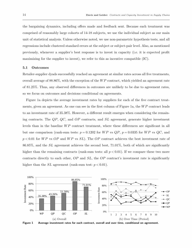
Retailer-supplier dyads successfully reached an agreement at similar rates across all five treatments,
overall average of 88.86%, with the exception of the WP contract, which yielded an agreement rate
of 81.25%. Thus, any observed differences in outcomes are unlikely to be due to agreement rates,
so we focus on outcomes and decisions conditional on agreements.
Figure 1a depicts the average investment rates by suppliers for each of the five contract treat-
ments, given an agreement. As one can see in the first column of Figure 1a, the WP contract leads
to an investment rate of 35.38%. However, a different result emerges when considering the remain-
ing contracts. The QP , QC, and OP contracts, and SL agreement, generate higher investment
levels than in the baseline WP contract treatment, where these differences are significant in all
but one comparison (rank-sum tests: p= 0.1202 for WP vs QP , p= 0.0335 for WP vs QC, and
p < 0.01 for WP vs OP and WP vs SL). The OP contract achieves the best investment rate of
86.85%, and the SL agreement achieves the second best, 71.01%, both of which are significantly
higher than the remaining contracts (rank-sum tests: all p < 0.01). If we compare these two more
contracts directly to each other, OP and SL, the OP contract’s investment rate is significantly
higher than the SL agreement (rank-sum test: p < 0.01).
35.38% 43.26%51.58%
86.85%
71.01%
0%
20%
40%
60%
80%
100%
WP QP QC OP SL
Inve
stm
ent R
ate
(a) Overall
9 10 1 2 3 4 5 6 7
103.75 105 26% 29% 64% 18% 38% 25% 25%104.5652 104.6154 52% 42% 24% 30% 29% 36% 33%106.8182 108.6842 35% 54% 45% 50% 48% 35% 27%107.1429 106.4286 45% 64% 50% 57% 52% 65% 43%112.8571 112.1429 86% 90% 92% 90% 85% 91% 83%
0.833333 0.833333 0.6 0.705882 0.611111 0.611111 0.666667
112.8571 112.1429 86% 90% 92% 90% 85% 91% 83%0.833333 0.833333 0.6 0.705882 0.611111 0.611111 0.666667
107.1429 106.4286 45% 64% 50% 57% 52% 65% 43%106.8182 108.6842 35% 54% 45% 50% 48% 35% 27%104.5652 104.6154 52% 42% 24% 30% 29% 36% 33%
earnings20132.425209.6
2695225641.6
26394.24Tl less 5 123179.8
5355.645game earn 23.28541end 28.28541
regressions for trendopen steve's "invest.do" filecombine the data using the same filextset subject periodxtlogit invest period if(contract==1)xtlogit invest period if(contract==2)xtlogit invest period if(contract==3)xtlogit invest period if(contract==4)xtlogit invest period if(contract==5)
0%
20%
40%
60%
80%
100%
1 2 3 4 5 6 7 8 9 10
Inve
stm
ent R
ate
Period
OPSLQCQPWP
(b) Over Time (Period)
Figure 1 Average investment rates for each contract, overall and over time, conditional on agreement.

Davis and Leider: Contracts and Capacity Investment in Supply Chains 15
The favorable investment rates of the OP contract and SL agreement appear to persist over time,
observed in Figure 1b. To formally check for any experience effects, we ran five Logit regressions
with clustered standard errors, with the supplier investment decision as the dependent variable,
and the decision period as the independent variable. The coefficient on the period variable was not
significantly different from zero in any of the five regressions (smallest p= 0.288).
Table 2 provides a summary of additional results. Beginning with incentive compatibility rates,
in Table 2, one can immediately recognize a difference between the OP contract and SL agreement,
compared to the remaining three contracts. That is, 91.55% of agreements in the OP contract
were incentive compatible, and 72.78% of the agreements in the SL agreement were incentive
compatible, compared to roughly half in the QC contract and only a minority in the WP and
QP contracts. Thus, the favorable investment rates of the OP contract and SL agreement may be
attributed to their ability to generate incentive compatible agreements.
Table 2 Summary of experimental results for each contract, outcomes conditional on agreement.
Contract % Agreement % ICRetailer Supplier Contract Terms
IC|wProfit Profit w/w1 w2 q po B
WP81.25% 12.82% 50.84 54.47 5.61 - - - - -
[2.70] [3.80] [1.62] [1.36] [0.11]
QP89.58% 21.86% 49.75 56.74 5.79 5.43 - - - w2 ≥ 7.00
[2.23] [4.01] [1.51] [1.45] [0.13] [0.16]
QC92.08% 51.58% 49.50 58.24 5.29 - 14.34 - - q≥ 13.97
[1.85] [4.21] [1.65] [1.83] [0.10] [0.31]
OP88.75% 91.55% 42.98 70.05 5.19 - - 27.55 - po ≥ 9.03
[2.61] [2.52] [3.72] [3.79] [0.14] [2.45]
SL93.89% 72.78% 43.54 67.11 5.09 - - - 25.90 B ≥ 19.06
[1.81] [4.55] [2.09] [1.89] [0.16] [1.81]
Note: Standard errors across subjects reported in square brackets. IC|w reports the average threshold for the secondparameter for incentive compatibility, given the observed wholesale prices in the data.
Turning to retailer and supplier expected profits, in Table 2, there appears to be a correlation
between investment rates and distribution of expected profits. For instance, the WP contract,
while yielding a relatively low level of investment, provides the most equitable payoffs between
the retailer and supplier: suppliers make roughly 3.63 more in expected profit than retailers. As
we move down the table, to those coordinating contracts which lead to higher investment rates,
this difference in expected profits only increases, from 3.63 in the WP contract, to 6.99 in the QP
contract, to 8.74 in the QC contract, to 27.07 in the OP contract, and 23.57 in the SL agreement.
These data suggest that contracts which increase overall supply chain profits disproportionably
favor the supplier. Indeed, compared to the WP contract, while suppliers earn considerably more in
the contracts generating higher investment, retailers actually begin to earn less in expected profit.

16 Davis and Leider: Contracts and Capacity Investment in Supply Chains
Table 2 also delineates the average contract parameters for agreements in each treatment, and the
average required condition on any secondary term for incentive compatibility, given the observed
wholesale price. Starting with the WP contract, the average agreed upon wholesale price was
5.61, below the required threshold for incentive compatibility (w ≥ 7.00). A similar result exists
in the QP contract, where subjects agreed on wholesale price of 5.79, but a secondary wholesale
price of only 5.43, considerably lower than the condition for incentive compatibility (w2 ≥ 7.00).
The QC contract performs a bit better in this regard, in that the average quantity commitment
was 14.34, which, given the observed wholesale prices (average 5.29), is higher than the average
quantity commitment required for incentive compatibility (q≥ 13.97). In the OP contract and SL
agreement, given the observed wholesale prices (average 5.19 in OP and 5.09 in SL), the agreed
secondary terms, the option fee and bonus, are far above the thresholds for incentive compatibility;
27.55 in the OP contract (po ≥ 9.03), and 25.90 in the SL agreement (B ≥ 19.06).
Lastly, in Table 2, the average wholesale prices for all five contracts are roughly halfway between
the retailer’s revenue per unit r = 10 and the suppliers cost of production c= 0. Keeping this in
mind, recall from Section 3 that the QP , QC, OP contracts, and SL agreement can all lead to
first-best investment while (nearly, for SL) equalizing expected profits. Specifically, this is possible
when 4.25≤ w1 ≤ 5.75 in the QP contract, 4.63≤ w ≤ 5.75 in the QC contract, and w ≤ 5.75 in
the OP contract (in the SL agreement, w≤ 4.5 is necessary, but w= 5 can also lead to relatively
equitable expected profits). Returning to Table 2, the average observed wholesale prices for these
contracts are within, or near, all of these ranges, suggesting that the secondary parameters may
be partly responsible for the considerable inequity we observe in certain contracts. For instance,
consider the OP contract, where the average option fee is 27.55. In Table 1, we observed that
the necessary option fee, assuming a wholesale price of 5, to induce investment and lead to equal
expected profits, is only po = 17.5. Thus, secondary terms, in those contracts that contribute to
higher rates of first-best investment, are one potential reason we observe the differences in expected
profits. We will investigate how subjects came to these types of agreements in the next subsection.
5.2 Bargaining Dynamics
We now turn to the bargaining data. Table 3 shows the number of messages sent per subject, by
minute (the average time to come to an agreement was around three minutes in each contract, with
the longest being three minutes 10 seconds in the WP contract). Looking at Table 3, there were
more messages sent about the wholesale price than the secondary parameter, particularly in the
QP and QC contracts. Although this effect is weaker in the SL agreement, which may be due to
the fact that the SL agreement is the only contract where the secondary parameter is potentially

Davis and Leider: Contracts and Capacity Investment in Supply Chains 17
paid even if the supplier does not invest (and demand is low). These data also suggest that subjects
did not take a sequential nature to bargaining, and instead sent feedback over both parameters
consistently over time, particularly about the wholesale price.
Table 3 Number of messages sent, per subject, per minute, for the coordinating contracts.
Contract Term Total First Second Third Fourth
QPw1 21.83 9.77 5.98 4.13 1.96
w2 9.40 5.19 2.35 1.23 0.63
QCw 28.06 11.65 7.44 5.40 3.58
q 9.79 4.21 2.79 1.92 0.88
OPw 25.04 10.83 7.19 4.81 2.21
p0 19.33 8.13 5.56 3.77 1.88
SLw 18.86 8.86 4.97 3.31 1.72
B 17.78 6.72 5.31 3.64 2.11
In Figure 2, we provide two arrow plots that illustrate the types of feedback sent for the QP
and QC contracts. In these plots the vertical axis represents the wholesale price, w or w1, and the
horizontal axis represents the secondary parameter, w2 or q. The origin of the arrows illustrates a
contract offer, rounded, and the length of the arrows depict the frequency in which messages were
sent about a parameter: longer (shorter) vertical arrows suggest many (few) messages were sent
only about the wholesale price, longer (shorter) horizontal arrows indicate many (few) messages
were sent only about the secondary parameter, and longer (shorter) arrows in a straight diagonal
suggest many (few) messages were sent equally about both parameters. Consistent with Table 3,
in Figure 2, for both plots, the majority of the arrows are vertical, and relatively long, implying
that feedback for contracts frequently consisted of messages focusing on the wholesale price being
too high (i.e. down arrow) or too low (i.e. up arrow). In fact, in both the QC and QP contract, it
appears that a vast majority of the messages focused on driving the wholesale price to around 5 (in
the OP contract and SL agreement, not depicted, similar effects persist, but are not as strong).
We now turn to how offers evolve over time. In Figure 3, we provide two sunflower density
plots for the QC contract and the SL agreement, which depict the contract proposals during
the bargaining stage at different moments in time (similar patterns exist for the QP and OP
treatments). Specifically, the left-hand side figures show the density of contract offers during the
first minute of bargaining, whereas the right-hand side figures show the density of contract offers
during the fourth minute of bargaining. The vertical axis denotes the wholesale price w, and the
horizontal axis represents the secondary parameter, q or B. One can immediately notice that

18 Davis and Leider: Contracts and Capacity Investment in Supply Chains
02
46
810
w1
0 2 4 6 8 10w2
(a) QP
02
46
810
w
10 12 14 16 18 20q
(b) QC
Figure 2 Arrow plots depicting the direction of contract offer feedback in the QP and QC contracts. The origin
of each arrow illustrates a contract offer, rounded, and the length of the arrows depict the frequency
in which messages were sent about a parameter: longer (shorter) vertical arrows suggest many (few)
messages sent only about the wholesale price, longer (shorter) horizontal arrows indicate many (few)
messages sent only about the secondary parameter, and longer (shorter) arrows in a straight diagonal
suggest many (few) messages sent equally about both parameters.
during the first minute of bargaining, there is considerable dispersion of offers for both parameters.
However, during the final minute, wholesale prices converge to around 5, whereas the secondary
parameters continue to exhibit considerable variability (a similar pattern emerges if you look at
the first and last two minutes). This suggests that subjects responded to the plethora of messages
about the wholesale price, and that they put in considerable effort in negotiating the wholesale
price, but gave relatively less attention to the secondary parameter.
In addition to the main bargaining results presented thus far, some other highlights include:
initial offers by both retailers and suppliers favored themselves considerably, suppliers tended to
make more incentive compatible offers than retailers, both retailers and suppliers failed to accept
offers that resulted in low expected profits for themselves, and 50% of all offers were made by
suppliers. None of these results are entirely surprising, and point to rational behavior in general.
5.3 “Superficial Fairness”
Thus far, one primary result is that the OP contract and SL agreement generate higher levels of
incentive compatible agreements and investment, but also highly inequitable payoffs. In regards
to the bargaining dynamics, we also observe that retailers and suppliers tend to (1) place more
emphasis on bargaining over the wholesale price, and (2) settle on a price that is roughly halfway
between the retailer’s revenue per unit and supplier’s cost of production per unit. Here, we provide

Davis and Leider: Contracts and Capacity Investment in Supply Chains 19
02
46
810
w
10 12 14 16 18 20q
1 petal = 1 obs. 1 petal = 6 obs.
(a) QC first minute
02
46
810
w
10 12 14 16 18 20q
1 petal = 1 obs. 1 petal = 6 obs.
(b) QC fourth minute
02
46
810
w
0 20 40 60 80B
1 petal = 1 obs. 1 petal = 6 obs.
(c) SL first minute
02
46
810
w
0 20 40 60 80B
1 petal = 1 obs. 1 petal = 6 obs.
(d) SL fourth minute
Figure 3 Sunflower density plots for the QC contract and SL agreement offers in the first and fourth minute. Each
circle represents a single observation. Each line on a lightly-shaded hexagon represents one observation.
Each line on a darkly-shaded hexagon represents six observations.
further support for these bargaining tendencies, and discuss how these two bargaining anomalies,
which we collectively refer to as “superficial fairness,” contribute to our experimental results.
There is a vast literature that shows when parties negotiate over a parameter with salient end-
points, the two parties often make concessions and come to an agreement that is roughly in the
middle (Roth and Malouf 1979, 1982). Indeed, in our experimental data, retailers and suppliers tend
to start with an initial offer which strongly favors themselves, and eventually settle on a wholesale
price that appears more equitable. Specifically, the average midpoint, between the retailer’s and
supplier’s first wholesale price offers, ranges from 5.01 in the SL agreement, to 5.73 in the QP
contract, and the wholesale price for accepted offers is significantly correlated with the midpoint
of the initial offers, in all treatments (ρ ranges from 0.377 in OP to 0.695 in QP , p < 0.01 for all).

20 Davis and Leider: Contracts and Capacity Investment in Supply Chains
The corresponding concession pattern for the secondary parameters, however, is not as strong.
While the secondary parameters for the accepted contract and the midpoint of the initial offers
are significantly correlated, the strength of the correlation is relatively weaker (ρ between 0.18
in SL to 0.53 in QP , p < 0.01 for all). Also, importantly, the secondary parameters for accepted
contracts significantly differ from the midpoint of initial offers in each treatment, other than QP
(signed-rank test: p= 0.47 in QP , p < 0.01 for all others).
To determine what contributes to accepting an offer, Table 4 reports the results of regressing
subjects’ acceptance of an offer using Logit regressions with subject-pair clustered standard errors.
IsIC is an indicator variable equalling 1 if the offer is incentive compatible. RiskDifference is
a risk allocation measure, where we first calculated the absolute difference in profits if demand
is high or low, for both the retailer and supplier (conditional on the correct investment choice),
and then took the absolute difference between the parties. This variable will be high if either
the retailer or supplier is bearing the majority of the payoff uncertainty, and will be zero if they
have equal payoff uncertainty. Similarly, Inequality captures the payoff inequality by taking the
absolute difference between the retailer’s and supplier’s expected profits (conditional on the correct
investment). Finally, w ∈ [4.5,5.5] is an indicator variable that equals 1 if the wholesale price is
between 4.50 and 5.50, capturing the superficial fairness of the offer (we obtain qualitatively similar
results if we use alternate measures of superficial fairness, such as expanding the range to w ∈ [4,6]).
In Table 4, in all contracts, offers are significantly more likely to be accepted if the wholesale
price is superficially fair. And the magnitude of the effect is considerable - increasing the likelihood
of acceptance by between one-third and two-thirds of the baserate probability (QP : 32%, QC:
66%, OP : 59%, SL: 52%). In contrast, subjects do not appear to favor offers that are incentive
compatible. Similarly, subjects do not seem to reject offers that are objectively unequal in either
expected profits or risk allocation, the former of which is consistent with our data in that contracts
with highly unequal expected profits are accepted. Finally, while not depicted, we note that there is
no corresponding preference for offers near the middle value of the secondary parameter, which can
directly contribute to the distribution of expected profits (in separate regressions, the coefficients
on an indicator variable for the secondary characteristics are not significant in any treatment).
This emphasis on the wholesale price, combined with concessions, can account for the rates
of incentive compatibility we observe, and also, qualitatively, the differences in expected profits.
As previously highlighted in Section 3, when both contract parameters are unconstrained, the
QP , QC, and OP contracts, and SL agreement, have considerable flexibility at inducing the
supplier to invest in capacity and equalize expected profits. However, if one of the two parameters

Davis and Leider: Contracts and Capacity Investment in Supply Chains 21
Table 4 Logit regressions of accepting an offer, for the QP , QC, and OP contracts, and SL agreement.
QP QC OP SL
(1) (2) (3) (4) (5) (6) (7) (8)
IsIC -0.612∗∗ -0.639∗∗ -0.0324 0.0719 0.375 -0.128 0.173 -0.0145
[0.257] [0.257] [0.263] [0.264] [0.272] [0.278] [0.207] [0.206]
RiskDifference 0.00384 0.00261 0.0.00359 4.02e-05 -0.00824 0.00464 0.00878 0.0250∗∗
[0.00893] [0.00893] [0.00345] [0.00352] [0.00565] [0.00577] [0.00692] [0.00802]
Inequality -0.00437 0.00238 -0.00772∗ 0.00135 0.00263 0.00215 -0.00640∗∗ -0.00681∗∗∗
[0.00404] [0.00467] [0.00405] [0.00373] [0.00207] [0.00191] [0.00254] [0.00222]
w ∈ [4.5,5.5] 0.428∗∗ 0.812∗∗∗ 0.782∗∗∗ 0.748∗∗∗
[0.180] [0.190] [0.195] [0.211]
T ime 0.0115∗∗∗ 0.0115∗∗∗ 0.00916∗∗∗ 0.00921∗∗∗ 0.0125∗∗∗ 0.0124∗∗∗ 0.0126∗∗∗ 0.0124∗∗∗
[0.00121] [0.00122] [0.00123] [0.00123] [0.00122] [0.00125] [0.00144] [0.00148]
Constant -3.514∗∗∗ -3.830∗∗∗ -3.330∗∗∗ -3.907∗∗∗ -4.395∗∗∗ -4.521∗∗∗ -3.963∗∗∗ -4.404∗∗∗
[0.229] [0.252] [0.247] [0.277] [0.317] [0.321] [0.278] [0.317]
Note: Logit regression with standard errors clustered at the subject-pair level. Dependent variable is the contractacceptance decision. IsIC is a binary variable equaling 1 when an offer was incentive compatible, RiskDifferencedenotes the absolute difference in payoff risk between the retailer and supplier, Inequality denotes the absolute differencein average payoffs between the retailer and supplier, , w ∈ [4.5,5.5] is a binary variable equaling 1 when the offeredwholesale price was between 4.50 and 5.50, and T ime shows the time in the round.
is restricted to a particular value, and the secondary parameter is overlooked, then the performance
of these contracts may differ. Specifically, if the average wholesale price in all contracts is w =
5, then the proportion of the contracting space for the secondary parameter that will lead to
incentive compatibility, or favor the supplier over the retailer, greatly differs across the contracts.
For example, in the QC contract, the quantity commitment parameter must be between 10 and
20, where the requirement for incentive compatibility is q≥ 14, and the requirement for a supplier
earning strictly more than the retailer in expected profits is q ≥ 17. This implies that 60% of the
quantity commitment parameter space, leads to incentive compatible outcomes, and 30% leads to
the supplier earning more in expected profits. Table 5 shows the results from applying this approach
to each of the coordinating contracts (focusing on the individually rational contract space for the
OP contract and SL agreement). As one can see, the ordering of incentive compatibility rates and
inequity of expected profits, is consistent with that which exists in the experimental data.
In summary, concessions indicate that during negotiations, players will tend to end up in the
middle of the potential contracting space. This, combined with the fact that subjects focus most of
their bargaining efforts over the wholesale price, and partially overlook the secondary parameter,
suggests that the OP contract, and a lesser extent the SL agreement, have a distinct advantage
in arriving at incentive compatible agreements. This, in turn leads to higher investment rates and
greater expected supply chain profits, but also significantly more expected profits for the supplier.
In fact, given a superficially fair agreement in our setting, we can demonstrate that for any set

22 Davis and Leider: Contracts and Capacity Investment in Supply Chains
Table 5 Analysis of superficial fairness on incentive compatibility rates and expected profit distribution.
ContractIncentive Compatibility πS ≥ πR, given IC
Requirement % Region∗ Requirement % Region∗
QP w2 ≥ 7.00 30% w2 ≥ 8.5 15%
QC q≥ 14 60% q≥ 17 30%
OP po ≥ 10 87% po ≥ 17.5 77%
SL B ≥ 20 73% B ≥ 20 73%Note: ∗ For the OP contract and SL agreement, these numbers reflect the region of the individually rational contractingspace (i.e. large option fees and bonuses may drive the retailer’s expected profit negative).
of parameters (that leads to a non-trivial capacity investment problem) the incentive compatible
region for superficially fair contracts will always be (weakly) largest for the OP contract. We
provide the proof in an online Appendix.
Proposition 1. For superficially fair contracts (w = r/2), the OP contract has an incentive
compatible region that is strictly larger than the incentive compatible region for QP contract and
SL agreement, and is weakly larger than the region for the QC contract.
6. Robustness Checks
In an effort to investigate the robustness of our results, we conducted two additional experimental
studies, consisting of five treatments and 190 additional subjects. In this section we detail the results
for these two robustness checks: one which evaluates a scenario where a superficially fair wholesale
price should, in theory, induce investment, and another which considers continuous demand.
6.1 Alternative Two-Point Demand
In our first robustness study, we evaluated a scenario in which a superficially fair wholesale price
is incentive compatible. To this end, we ran one treatment of the WP contract (42 subjects) and
one treatment of the OP contract (40 subjects) with one subtle difference compared to our main
study: the probability of high demand occurring was increased from 1/2 to 7/10, thus making w= 5
incentive compatible for the supplier. All other parameters and experimental protocols remained
the same. Conducting these treatments helps determine (a) whether the favorable performance of
the OP contract, from a supply chain perspective, persists in an alternative setting, (b) whether
there continues to be a wider distribution of expected profits in the OP contract, and (c) more
importantly, whether investment levels in the WP contract increase in this new scenario, relative
to the main experiment, supporting the superficial fairness hypothesis.
In these two new treatments, dyads came to an agreement 83.81% of the time in the WP
treatment and 89% in the OP treatment, which yields a weak statistically significant difference

Davis and Leider: Contracts and Capacity Investment in Supply Chains 23
(rank-sum test: p= 0.096). Note that these rates are virtually identical to those in the main study
(previously 81.25% in the WP contract, and 88.75% in the OP contract). As with our analysis
of the main experiment, we report outcome results conditional on an agreement. A summary of
additional results is provided in Table 6.
Table 6 Summary of results for the two-point demand robustness study, outcomes conditional on agreement.
% Agreement % Investment % ICRetailer Supplier Terms Messages
Profit Profit w p0 w p0
WP83.81% 68.18% 80.11% 59.89 63.97 5.86 - 52.38 -
[3.32] [4.91] [4.22] [3.02] [2.65] [0.17]
OP89.00% 93.82% 98.31% 48.31 84.52 5.23 32.60 26.83 22.50
[3.26] [3.80] [1.08] [4.75] [4.96] [0.19] [5.07]Note: Standard errors across subjects reported in square brackets.
One observation from Table 6 is that, consistent with the main experiment, the OP contract
yields higher investment levels and more incentive compatible agreements than the WP contract
(93.82% versus 68.18% investment, and 98.31% versus 80.11% incentive compatibility, both rank
sum tests: p < 0.01). In addition, we see a significant improvement in investment and incentive
compatibility rates over the main experiment. Specifically, average investment rates in the WP
contract double from 35.38% previously to 68.18%, and incentive compatibility rates increase from
12.82% previously to 80.11%. This result is qualitatively in line with superficial fairness, since
w = 5 is now incentive compatible. The OP contract also has higher investment rates (93.82%
versus 86.85% previously, rank sum p= 0.04) and more frequent incentive compatible agreements
(98.31% versus 91.55% previously, rank sum p= 0.07). Overall, the OP contract still yields the best
outcomes for the supply chain, but the relative advantage of OP over WP is greatly diminished.
Turning to the distribution of expected profits between retailers and suppliers, in Table 6 it
appears that the OP contract provides more inequitable payoffs, despite its favorable performance
at inducing investment from suppliers, which is consistent with the main study.
Continuing in Table 6, wholesale prices are similar to those in the main study: 5.86 versus 5.61
previously in the WP contract, and 5.23 versus 5.19 previously in the OP contract. There is a small
difference in the option fee, which increases to 32.60 from 27.55 previously. Lastly, the bargaining
dynamics are consistent with the main study, in that the number of messages sent about each
parameter only slightly favored the wholesale price in the OP contract, 26.83, compared to the
option fee, 22.50 (previously 25.04 for the wholesale price and 19.33 for the option fee).

24 Davis and Leider: Contracts and Capacity Investment in Supply Chains
To summarize this robustness study, we find that when a superficially fair wholesale price is
incentive compatible, investment rates increase significantly for both contracts. Strikingly, com-
pared to our main study, average investment rates in the WP contract nearly double in this new
scenario. Furthermore, the qualitative results from the main study continue to hold: the OP con-
tract still yields the most incentive compatible agreements and achieves high investment levels,
nearly 94% given an agreement, and these supply chain benefits continue to entirely favor the
supplier.
6.2 Continuous Demand
In our second robustness study, we consider a scenario in which demand is continuous. To this end,
we implemented the same experimental protocols as in our main study, but allow for demand to
be uniformly distributed from 10 to 20, and set the cost of increasing supply capacity, k ∈ [10,20],
by one unit, to 3.5 (thus, as in our main study, an investment of 35 would increase capacity from
10 to 20). Under this continuous demand scenario we explored the WP , QC, and OP contracts,
where each treatment consisted of three sessions (42, 32, and 34 subjects).
6.2.1 Continuous Demand Theory Before presenting our experimental results, we first
review some of the theoretical details of the WP , QC, and OP contracts for demand following
a continuous distribution over [a, b], and k ∈ [a, b], along with some comments pertaining to our
experimental implementation of continuous demand (i.e. uniformly distributed between 10 and 20).
Before turning to each individual contract, we note that the supply chain expected profit under
continuous demand is given by:
πSC(k) =
∫ k
a
rxdF (x) + rk(1−F (k))− 3.5(k− a).
Which, for our continuous implementation, leads to a first-best investment level of k∗FB = 16.5,
with expected supply chain profit increasing from 100 (absent any investment, k= 10) to 121.125
(k= 16.5).
Let πji (x) denote the expected profit function of party i, i ∈ {R,S}, in contract j, j ∈
{WP,QC,OP} under continuous demand, where decision k is the supplier’s investment decision,
k ∈ [a, b]. Let k∗S denote the supplier’s optimal investment decision, conditional on the contract
parameters. Turning to the WP contract, each party’s expected profits are given by:
πWPR (k) =
∫ k
a
(r−w)xdF (x) + (r−w)k(1−F (k)),
πWPS (k) =
∫ k
a
wxdF (x) +wk(1−F (k))− 3.5(k− a).

Davis and Leider: Contracts and Capacity Investment in Supply Chains 25
For our experimental continuous parameters, in the WP contract the supplier’s optimal invest-
ment k∗S(w) = max[20− 35/w,10], such that the first-best investment level is only achieved when
w= 10. If we assume that superficial fairness exists, then w= 5 cannot lead to first-best investment,
and instead will lead to investment levels of k= 13, and the corresponding expected profits will be
πWPR = 52.25, and πWP
S = 62.75.
In the QC contract under continuous demand, if the supplier invests enough in capacity to satisfy
a quantity commitment k≥ q, then the retailer promises to purchases q units, regardless of demand.
If the supplier does not invest enough to satisfy the quantity commitment, k < q, then the quantity
commitment is not binding, and the two party’s transact at the agreed upon wholesale price. Note
that if w≥ 3.5 it is optimal for the supplier to set k≥ q. Assuming this, the corresponding party’s
expected profit functions under the QC contract with continuous demand are given by:
πQCR (k) =
∫ q
a
(rx−wq)dF (x) +
∫ k
q
(r−w)xdF (x) + (r−w)k(1−F (k)),
πQCS (k) =wqF (q) +
∫ k
q
wxdF (x) +wk(1−F (k))− 3.5(k− a).
For our continuous implementation in the QC contract, k∗S(w,q) = max[20− 35/w, q], implying
that it can achieve a first-best investment level if w ≥ 3.5 and q = 16.5. In terms of distributing
expected profits, a number of combinations can achieve first-best capacity investment with equal
expected profits. For instance, w∗ ∼ 5.05, will generate πQCR = 60.56 and πQC
S = 60.56.
In the OP contract, as noted in Section 3, the level of complexity for a general contract increases
considerably, compared to two-point demand. In particular, the OP contract under continuous
demand would consist of an option fee po paid by the retailer for the option to buy up to qo units at
wholesale price wo, with any additional units purchased at an increased wholesale price w. If k < qo
(i.e. the supplier cannot satisfy all of the options), then the option fee is returned, and the two
parties transact under a single wholesale price at wo. Assuming that the supplier invests enough in
capacity to satisfy the agreed upon number of options, k≥ qo, the expected profit functions under
the OP contract are given by:
πOPR (k) =
∫ qo
a
(r−wo)xdF (x) +
∫ k
qo
(r−w)xdF (x) + (r−w)k(1−F (k))− po,
πOPS (k) =
∫ qo
a
woxdF (x) +
∫ k
qo
wxdF (x) +wk(1−F (k)) + po− 3.5(k− a).
In our implementation of the OP contract, to limit complexity and avoid having subjects nego-
tiate over four contract parameters, we exogenously fix w= 1.2wo. That is, the increased wholesale

26 Davis and Leider: Contracts and Capacity Investment in Supply Chains
price for additional units beyond the options is always 20% higher than the negotiated option whole-
sale price. Subjects therefore negotiate over three contract parameters: wo, po, qo. In the continuous
OP treatment, k∗S(w,po, qo) = max[20− 35/w, qo]. Note that k∗S = qo is binding if w≤ 35/(20− qo).
Therefore if qo = 16.5 then k∗S = 16.5, which is the first-best investment level, for any w≤ 10. Many
combinations of parameters exist such that the expected profits of the two parties are equalized.
For example, if wo = 5, qo = 16.5, and po = 5.6, then both parties earn expected profits of 60.56.
As with our two-point demand setting, in the continuous demand case we expect the wholesale
price contract to lead to sub-optimal investment. Both the quantity commitment and option con-
tracts can, with the appropriate parameters, generate first best investment and equalize expected
profits. Additionally, both contracts can perform very well with the intuitive contract parameters
of a (discounted) wholesale price of 5 and a quantity commitment/number of options of 16.5. This
setting therefore provides a natural extension and robustness check of the findings of our main
experiment in a more general and realistic setting.
Lastly, in our experimental implementation, given the additional complexity of these contracts
with continuous demand, we provided subjects with a decision support tool during negotiations
and when making capacity decisions. During bargaining they could enter in potential contract
terms, and see each party’s expected profits for each level of investment in capacity. They could
also utilize this tool for any offers they received while bargaining. When making capacity decisions,
suppliers could see the expected profits for each level of investment given the agreed upon contract.
6.2.2 Continuous Demand Results Agreement rates in the WP , QC, and OP contracts
were 90.48%, 94.38%, and 90%, with no significant differences (all rank sum tests: p > 0.10). There-
fore, we continue to report outcomes conditional on an agreement. Also, we define the efficiency
gain from investment level k as the ratio between the increase in supply chain profit at the observed
investment over no investment (πSC(k)− πSC(10)), relative to the potential gains under first-best
investment (πSC(16.5)− πSC(10)). Hence, the ratio shows the percent of potential gains achieved.
Figure 4 depicts the efficiency gain for each of the contracts under continuous demand. As one
can see, in Figure 4 we have the familiar ranking of relative performance from a supply chain
perspective: the WP generates the lowest efficiency gains, the QC contract performs significantly
better, and the OP contract yields the best performance (rank-sum tests: all p < 0.01). However,
it is important to note that with continuous demand the magnitude of these differences have
diminished considerably compared to the main experiment. In other words, the differences across
contracts appear to be larger in a two-point demand setting, and slightly lessened with continuous

Davis and Leider: Contracts and Capacity Investment in Supply Chains 27WP 69.93% 0.033682QC 80.57% 0.029711OP 88.61% 0.025629
% Achieved 69.93%
80.57%88.61%
0%
20%
40%
60%
80%
100%
WP QC OP
Effic
ienc
y G
ain
Figure 4 Average efficiency gains in the continuous demand robustness study, conditional on agreement.
demand. This is in part due to the shape of the payoff function under continuous demand, with
diminishing returns as the investment approaches the first best level.
Table 7 provides a summary of additional results for the continuous robustness treatments. As
with the main study and first robustness check, it appears that the contracts which perform best at
achieving greater supply chain profits also yield fairly uneven expected profits between the retailer
and supplier. Specifically, under continuous demand, the supplier expected profit exceeds that of
the retailer by 2.24 in the WP contract, 3.47 in the QC contract, and 18.82 in the OP contract.
The observed payoff inequality is especially interesting given that both parties could easily see both
parties’ expected profits under various contracts using the decision support tool. This suggests that
equalizing expected payoffs was not a primary concern for many subjects.
With respect to contract terms and bargaining dynamics, in Table 7 we see a similar pattern,
consistent with the salience of superficial fairness, as in the main study and first robustness check.
Specifically, wholesale prices (wo for the OP contract) are around, or slightly above, the superficially
fair focal value of w= 5. Additionally, for the contracts with multiple parameters, far more messages
(per subject) were sent about the wholesale price than messages about the alternative parameters.
Table 7 Summary of results for the continuous demand robustness study, outcomes conditional on agreement.
Contract% Investment Retailer Supplier Contract Terms Messages
Agreement Level Profit Profit w/wo q qo po w/wo q qo po
WP90.48% 13.81 56.27 58.51 5.57 - - - 58.69 - - -
[2.12] [0.26] [0.88] [0.94] [0.07]
QC94.38% 14.30 56.78 60.25 5.37 14.65 - - 26.50 6.06 - -
[1.61] [0.22] [1.11] [1.29] [0.08] [0.18]
OP90.00% 15.38 49.95 68.77 4.98 - 15.59 16.09 14.38 - 6.91 8.29
[2.76] [0.24] [1.74] [1.91] [0.08] [0.19] [1.28]
Note: Standard errors across subjects reported in square brackets.

28 Davis and Leider: Contracts and Capacity Investment in Supply Chains
Together the results confirm the main results of our experiment in this more general setting.
Qualitatively, we see the same performance ranking across contracts, and we see a similar pattern
of bargaining and agreements. Superficial fairness seems to play an important role, and supply
chain efficiency appears to be tied to payoff inequality.
7. Conclusion
In this study, we conduct an experimental investigation of capacity investment problems with
bargaining. We compare five contracts that, in theory, can provide sufficient incentives and generate
first-best investment in capacity by the supplier: wholesale price, quantity premium, quantity
commitment, option, and service-level agreement. Further, four of these contracts can not only
provide proper incentives for first-best investment, but can also equalize expected profits between
the two parties. We find, however, that there are significant differences in the performance of
these contracts when we allow human-decision makers to bargain over contract terms and make
investment decisions. In particular, the option contract and service-level agreement significantly
outperform the other contracts in terms of first-best investment levels and thus supply chain profits.
These same contracts also generate the greatest inequity between the two parties in terms of
expected profits; the gains they generate in supply chain profit go entirely to the supplier.
In our experiment, we introduce a form of bargaining which puts some structure on the communi-
cation, but leaves the offer process unstructured. This allows us to observe the bargaining dynamics
over time. These data indicate that subjects have preferences for what we refer to as “superficial
fairness.” That is, subjects focus heavily on negotiating the wholesale price and eventually agree on
a wholesale price that is near the middle of the contracting space, while paying less attention to the
secondary term. These biases significantly distort the incentives provided by the quantity premium
and quantity commitment contracts. In contrast, the option contract and service-level agreement
have incentives that are robust to an over-emphasis on superficially fair wholesale prices, in terms
of first-best investment. However, these contracts are also more susceptible to superficial fairness
in terms of the distribution of payoffs, and, as a result, largely favor the supplier.
The tendency to focus on bargaining over one salient term is not uncommon in the bargaining
literature - often due to negotiators using sequential agendas that make joint gains hard to find
(Mannix et al. 1989), or by focusing on distributing value rather than finding integrative solutions
- the “mythical fixed pie” (Bazerman and Neale 1994). This behavior has also been observed in
practice. For instance, Devlin et al. (2014) conduct interviews with fashion retailers and suppliers
negotiating buyback contracts and find that “wholesale prices charged are similar regardless of the

Davis and Leider: Contracts and Capacity Investment in Supply Chains 29
presence of a buyback,” as if the buyback amount is largely overlooked. Nevertheless, while we
believe that this type of bargaining behavior is useful in the organizing the data, we admit that
there are undoubtedly many other dynamics taking place in the bargaining process which may
drive particular results.
We believe that there are several opportunities for future research in this area. One direction
would be to extend our work in a repeated setting. As mentioned previously, relational incentives
in a long-term relationship is a common solution to capacity investment problems. It would also
be interesting to extend our setting and results to incorporate renegotiation.
One limitation of our study is that subjects had a limited time to bargain over parameters.
While we believe our contractual setting was relatively simple compared to negotiations in practice
- most supply chain contracts would be significantly more complicated and deal with far greater
uncertainty and ambiguity - we recognize that many supply chain negotiations would likely involve
a greater length of time, and some additional level of calculations for each offer (although we
provided decision support in our continuous demand treatments). However, while this may be a
limitation to our study, we believe that ours is one of the first to allow both parties to make back-
and-forth offers, while also allowing them to provide limited feedback, as opposed to a setting with
only one-shot ultimatum offers. Thus, we believe that our work takes an important step towards
understanding a more realistic bargaining setting, but admit that more work is necessary to fully
understand capacity investment decisions and bargaining.
From a managerial standpoint, while we investigate a capacity investment context for the sup-
plier, our results can apply to smaller scale settings as well, where a supplier must make a
relationship-specific investment. For instance, a startup may need to invest in training, software, or
hiring specialized personnel, to serve a potential buyer. In these situations, our results suggest that
contracts similar to the option or service-level agreements may generate the optimal investment
by the supplier, and lead to increased supply chain profits, but may disproportionately favor the
supplier as well.
Acknowledgments
The authors would like to thank seminar participants at the University of Southern California, Cornell Uni-
versity, Union College, 2013 Behavioral Operations Conference, and 2013 and 2014 INFORMS Conference.
They are also grateful for financial support from the Johnson School at Cornell University and the Ross
School of Management at the University of Michigan.

30 Davis and Leider: Contracts and Capacity Investment in Supply Chains
References
Al-Ubaydli, Omar, Steffen Andersen, Uri Gneezy, John A. List. 2015. Carrots that look like sticks: Toward
an understanding of multitasking incentive schemes. Southern Economic Journal 81(3) 538–561.
Babcock, Linda, George Loewenstein. 1997. Explaining bargaining impasse: the role of self-serving biases.
Journal of Economic Perspectives 11(1) 109–126.
Baker, George. 1992. Incentive contracts and performance measurement. Journal of Political Economy 100
598–614.
Baker, George, Robert Gibbons, Kevin J. Murphy. 2002. Relational contracts and the theory of the firm.
Quarterly Journal of Economics 117 3983.
Bazerman, Max H., Jared R. Curhan, Don A. Moore, Kathleen L. Valley. 2000. Negotiation. Annual Review
of Psychology 51 279–314.
Bazerman, Max H., Margaret A. Neale. 1994. Negotiating Rationally . New York: The Free Press.
Becker-Peth, Michael, Ulrich W. Thonemann. 2016. Reference points in revenue sharing contracts - how to
design optimal supply chain contracts. European Journal of Operations Research 249(3) 1033–1049.
Bolton, Gary, Axel Ockenfels. 2000. Erc: A theory of equity, reciprocity, and competition. American Economic
Review 90(1) 166–193.
Cachon, Gerard P., Martin A. Lariviere. 2001. Contracting to assure supply: How to share demand forecasts
in a supply chain. Management Science 47(5) 629–646.
Camerer, Colin. 2003. Behavioral game theory: Experiments in strategic interaction. Princeton University
Press, Princeton, NJ.
Chung, Tai-Yeong. 1991. Incomplete contracts, specific investment and risk sharing. Review of Economic
Studies 58(5) 1031–1042.
Coase, Ronald. 2006. The conduct of economics: The example of fisher body and general motors. Journal
of Economics & Management Strategy 15(2) 255–278.
Davis, Andrew M., Elena Katok, Natalia Santamarıa. 2014. Push, pull, or both? a behavioral study of how
the allocation of inventory risk affects channel efficiency. Management Science 60(11) 2666–2683.
Devlin, Anna, Rebecca Hamilton, Wedad Elmaghbraby. 2014. Understanding the appeal of suboptimal
contracts. Working Paper, University of Maryland .
Dufwenberg, Martin, Alec Smith, Mat Van Essen. 2013. Hold-up: With a vengeance. Economic Inquiry 51
896–908.
Ellingsen, Tore, Magnus Johannesson. 2004. Is there a hold-up problem? The Scandinavian Journal of
Economics 106(3) 475–494.
Fehr, Ernst, Susanne Kremhelmer, Klaus M. Schmidt. 2008. Fairness and the optimal allocation of ownership
rights. Economic Journal 118(531) 1262–1284.

Davis and Leider: Contracts and Capacity Investment in Supply Chains 31
Fehr, Ernst, Klaus M. Schmidt. 1999. A theory of fairness, competition, and cooperation. The Quarterly
Journal of Economics 114(3) 817–868.
Fehr, Ernst, Klaus M. Schmidt. 2004. Fairness and incentives in a multi-task principal-agent model. The
Scandanavian Journal of Economics 106(3) 453–474.
Fischbacher, Urs. 2007. z-Tree: Zurich toolbox for ready-made economic experiments. Experimental Eco-
nomics 10(2) 171–178.
Fukuno, Mitsuteru, K-I Ohbuchi. 1997. Cognitive biases in negotiation: the determinants of fixed-pie assump-
tion and fairness biases. Japanese Journal of Social Psychology 13(1) 43–52.
Grossman, Sanford J., Oliver D. Hart. 1986. The costs and benefits of ownership: A theory of vertical and
lateral integration. Journal of Political Economy 94(4) 691–719.
Guth, Werner, Rolf Schmittberger, Bernd Schwarze. 1982. An experimental analysis of ultimatum bargaining.
Journal of Economic Behavior and Organization 3(4) 367–388.
Guth, Werner, Reinhard Tietz. 1990. Ultimatum bargaining behavior: A survey and comparison of experi-
mental results. Journal of Economic Psychology 11(3) 417–449.
Hart, Oliver, John Moore. 1990. Property rights and the nature of the firm. Journal of Political Economy
98 1119–1158.
Holmstrom, Bengt, Paul Milgrom. 1991. Multitask principal-agent analyses: incentive contracts, asset own-
ership and job design. Journal of Law, Economics and Organization 7 24–52.
Hoppe, Eva I., Patrick W. Schmitz. 2011. Can contracts solve the hold-up problem? experimental evidence.
Games and Economic Behavior 73 186–199.
Kerr, Steven. 1975. On the folly of rewarding a, while hoping for b. The Academy of Management Journal
18(4) 769–783.
Klein, Benjamin. 2007. The economic lessons of fisher bodygeneral motors. International Journal of the
Economics of Business 14(1) 1–36.
Klein, Benjamin, Robert G. Crawford, Armen A. Alchian. 1978. Vertical integration, appropriable rents,
and the competitive contracting process. Journal of Law and Economics 21(2) 297–326.
Klein, Benjamin, Keith B. Leffler. 1981. The role of market forces in assuring contractual performance.
Journal of Political Economy 89(4) 615–641.
Leider, Stephen G., William S. Lovejoy. 2016. Bargaining in supply chains. Management Science 62(10)
3039–3058.
Lovejoy, William S. 2010. Conversations with supply chain managers. Working Paper, University of Michigan
.
Mannix, Elizabeth A., Leigh L. Thompson, Max H. Bazerman. 1989. Negotiation in small groups. Journal
of Applied Psychology 74(3) 508–517.

32 Davis and Leider: Contracts and Capacity Investment in Supply Chains
McFadden, Daniel. 1974. Conditional logit analysis of qualitative choice behavior. Paul Zarembeka, ed.,
Frontiers in Econometrics. Academic Press, New York, 105–142.
McKelvey, Richard D., Thomas R. Palfrey. 1995. Quantal response equilibrium for normal form games.
Games and Economic Behavior 10 6–38.
Muthoo, Abhinay. 1999. Bargaining Theory with Applications. Cambridge: Cambridge University Press.
Nash, John. 1950. The bargaining problem. Econometrica 18(2) 155–162.
Oblicore. 2007. 2007 service-level management survey: Results, trends and analysis. Tech. rep., Oblicore,
Inc.
Ozer, Ozalp, Wei Wei. 2006. Strategic commitment for optimal capacity decision under asymmetric forecast
information. Management Science 52(8) 1238–1257.
Philipson, Thomas, Thomas Lawless. 1997. Multiple-output agency incentives in data production: experi-
mental evidence. European Economic Review 41(3) 961–970.
Plambeck, Erica L., Terry A. Taylor. 2005. Sell the plant? the impact of contract manufacturing on innova-
tion, capacity, and profitability. Management Science 51(1) 133–150.
Plambeck, Erica L., Terry A. Taylor. 2007. Implications of renegotiation for optimal contract flexibility and
investment. Management Science 53(12) 1872–1886.
Roth, Alvin E. 1995. Bargaining experiments. John Kagel, Alvin E. Roth, eds., Handbook of Experimental
Economics. Princeton University Press, Princeton, NJ, 253–348.
Roth, Alvin E., Michael W. K. Malouf. 1979. Game-theoretic models and the role of information in bargain-
ing. Psychological Review 86(6) 574–594.
Roth, Alvin E., Michael W. K. Malouf. 1982. The role of information in bargaining: An experimental study.
Econometrica 50 1123–1142.
Roth, Alvin E., Michael W. K. Malouf, J. Keith Murnighan. 1981. Sociological versus strategic factors in
bargaining. Journal of Economic Behavior and Organization 2(2) 153177.
Rubenstein, Ariel. 1982. Perfect equilibrium in a bargaining model. Econometrica 50(1) 97–109.
Scheele, Lisa M., Marco Slikker, Ulrich W. Thonemann. 2014. Designing incentive systems for truthful
demand information sharing - theory and experiment. Working Paper, University of Cologne .
Sloof, Randolph. 2008. Price-setting power vs. private information: An experimental evaluation of their
impact on holdup. European Economic Review 52 469486.
Sloof, Randolph, Joep Sonnemans, Hessel Oosterbeek. 2004. Specific investments, holdup, and the outside
option principle: an experimental study. European Economic Review 48 13991410.
Stuckey, John, David White. 1993. When and when not to vertically integrate. McKinsey Quarterly http:
// www. mckinsey. com/ insights/ strategy/ when_ and_ when_ not_ to_ vertically_ integrate .

Davis and Leider: Contracts and Capacity Investment in Supply Chains 33
Taylor, Terry A., Erica L. Plambeck. 2007. Simple relational contracts to motivate capacity investment:
Price only vs. price and quantity. Manufacturing & Service Operations Management 9(1) 94–113.
Thompson, Leigh L., Terri DeHarpport. 1990. Social judgment, feedback, and interpersonal learning in
negotiation. Organizational Behavior and Human Decision Processes 58(3) 327–345.
Thompson, Leigh L., Reid Hastie. 1990. Social perception in negotiation. Organizational Behavior and
Human Decision Processes 47(1) 98–123.
Thompson, Leigh L., Dennis Hrebec. 1996. Loselose agreements in interdependent decision making. Psycho-
logical Bulletin 120(3) 396–409.
Thompson, Leigh L., George Loewenstein. 1992. Egocentric interpretations of fairness and interpersonal
conflict. Organizational Behavior and Human Decision Processes 51(2) 176–197.
Tomlin, Brian. 2003. Capacity investments in supply chains: Sharing the gain rather than sharing the pain.
Manufacturing & Service Operations Management 5(4) 317–333.
Weingart, Laurie R., Rebecca J. Bennett, Jeanne M. Brett. 1993. The impact of consideration of issues and
motivational orientation on group negotiation process and outcomes. Journal of Applied Psychology
78(3) 504–517.
Williamson, Oliver E. 1979. Transactions-cost economics: the governance of contractual relations. Journal
of Law and Economics 22 23362.

34 Davis and Leider: Contracts and Capacity Investment in Supply Chains
Appendix A: Incentive Compatibility Region for Superficially Fair Contracts
We now consider the size of the incentive compatibility (IC) regions within our model for the OP , QC,
and QP contracts, and SL agreement, that are superficially fair (i.e. where w = r/2). We maintain the
underlying structure of the model (e.g. two-point demand, binary investment decision, etc.), but consider
variations in the parameters of the model (d,D, r, p,K). For the investment problem to be non-trivial, we
maintain throughout that K < rpδ < 2K (so for example an equal split of the surplus in ex post negotiation
would not be incentive compatible, similarly, a superficially fair wholesale price contract will not be incentive
compatible on its own). We begin by reformulating the IC and individually rational (IR) constraints to
separate out the common factors across contracts, given that w= r/2.
For the OP contract, the IC constraint is po ≥K − pwδ, or 2po ≥ 2K − rpδ. Define Θ = 2K − rpδ, which
represents the additional incentives that the secondary term in the contract must provide, given the incentives
that the wholesale price is already generating. Note that 0<Θ<K. The IC constraint is therefore po ≥Θ/2.
The retailer’s expected profit given the contract (and investment) is
(1− p)(r−w)d+ p(r−w)D− po = (r/2)(d+ pδ)− po.
Define Γ = (r/2)(d+pδ), which denotes the retailer’s remaining surplus given the wholesale price. Note that
Γ > Θ. The IR constraint is therefore po ≤ Γ. The size of the IC region for the OP contract is therefore
1−Θ/2Γ. Finally, since Γ>Θ, the size of the IC region is at least 50%.
For the SL agreement, by similar logic the IC constraint is po ≥ Θ/2p and the IR constraint is po ≤ Γ.
Therefore the size of the IC region is 1−Θ/2pΓ, which is strictly smaller than the OP contract’s IC region.
For the QC contract, we can rewrite the IC constraint as pwδ+(1−p)w(q−d)≥K or (1−p)r(q−d)≥Θ.
Finally, we can write the IC constraint as (q−d)≥Θ/r(1−p). Note that 0≤ (q−d)≤ δ. For the IR constraint
we can write the retailer’s expected profit as
(1− p)(r−w)d+ p(r−w)D− (1− p)w(q− d) = Γ− (1− p)w(q− d).
The IR constraint is therefore (q− d)≤ 2Γ/r(1− p). Note that there are two cases. In Case 1, this limit is
larger than δ, hence the IR constraint will not bind. In Case 2, 2Γ/r(1−p)< δ, which occurs if d< (1−2p)δ.
In Case 1 the size of the IC region of the QC contract is 1−Θ/rδ(1− p), while in Case 2 it is 1−Θ/2Γ.
Is it possible for the IC region for the QC contract to be larger than the OP contract? We take the two
cases in turn. For Case 1, we want to see if 1−Θ/rδ(1− p)> 1−Θ/2Γ. This would occur if 2Γ< rδ(1− p),
or d< (1− 2p)δ - however this violates the assumption that we are in Case 1. Therefore, for Case 1 the OP
contract always has a larger IC region than the QC contract. For Case 2, both contracts have the same size
region: 1−Θ/2Γ. Therefore, the size of the IC region for the OP contract is always at least weakly larger
than the size of the IC region for the QC contract.
For the QP contract, we know that we at least need w2 > r/2 (since we have assumed that the problem
is not trivially solved by a superficially fair wholesale price contract). Since w2 ∈ [0, r] is the IR region, the
IC region is no larger than 50% of the contracting space. Therefore, the OP contract always has a strictly

Davis and Leider: Contracts and Capacity Investment in Supply Chains 35
larger IC region than the QP contract. Taking all of these results, we can state that for superficially fair
contracts (w = r/2), the OP contract has an incentive compatible region that is strictly larger than the
incentive region for QP contract and SL agreement, and is weakly larger than the region for QC contracts.
Top Related