


Languages
Pages
Legal


Full Terms & Conditions of access and use can be found athttp://www.tandfonline.com/action/journalInformation?journalCode=uasa20
Download by: [Harvard Library] Date: 11 September 2015, At: 07:45
Journal of the American Statistical Association
ISSN: 0162-1459 (Print) 1537-274X (Online) Journal homepage: http://www.tandfonline.com/loi/uasa20
An Adaptive Exchange Algorithm for Samplingfrom Distributions with Intractable NormalizingConstants
Faming Liang, Ick Hoon Jin, Qifan Song & Jun S. Liu
To cite this article: Faming Liang, Ick Hoon Jin, Qifan Song & Jun S. Liu (2015): An AdaptiveExchange Algorithm for Sampling from Distributions with Intractable Normalizing Constants,Journal of the American Statistical Association, DOI: 10.1080/01621459.2015.1009072
To link to this article: http://dx.doi.org/10.1080/01621459.2015.1009072
View supplementary material
Accepted online: 06 Feb 2015.
Submit your article to this journal
Article views: 133
View related articles
View Crossmark data
ACCEPTED MANUSCRIPT
An Adaptive Exchange Algorithm for Sampling fromDistributions with Intractable Normalizing Constants
Faming Liang∗, Ick Hoon Jin, Qifan Song, and Jun S. Liu
Abstract
Sampling from the posterior distribution for a model whose normalizing constant is intractable is
a long-standing problem in statistical research. We propose a new algorithm, adaptive auxiliary
variable exchange algorithm, or in short, adaptive exchange (AEX) algorithm, to tackle this prob-
lem. The new algorithm can be viewed as a MCMC extension of the exchange algorithm (Murray,
Ghahramani and MacKay, 2006), which generates auxiliary variables via an importance sampling
procedure from a Markov chain running in parallel. The convergence of the algorithm is estab-
lished under mild conditions. Compared to the exchange algorithm, the new algorithm removes
the requirement that the auxiliary variables must be drawn using a perfect sampler, and thus can be
applied to many models for which the perfect sampler is not available or very expensive. Compared
to the approximate exchange algorithms, such as the double Metropolis-Hastings sampler (Liang,
2010), the new algorithm overcomes their theoretical difficulty in convergence. The new algorithm
is tested on the spatial autologistic and autonormal models. The numerical results indicate that the
new algorithm is particularly useful for the problems for which the underlying system is strongly
dependent.
Keywords: Autologistic Model; Exchange Algorithm; Intractable Normalizing Constant; Stochas-
tic Approximation Monte Carlo.∗To whom correspondence should be addressed. Liang is Professor, Department of Biostatistics, University of
Florida, Gainesville, FL 32611. Email: [email protected]. Jin is Research Scientist, Center for Biostatistics, The OhioState University, Columbus, Ohio 43221. Song is Assistant Professor, Department of Statistics, Purdue University,West Lafayette, IN 47906. Liu is Professor, Department of Statistics, Harvard University, Science Center 715, 1Oxford Street, Cambridge, MA 02138. Liang’s research was partially supported by grants from the National ScienceFoundation DMS-1106494 and DMS-1317131. The authors thank the editor, associate editor and two referees fortheir constructive comments which have led to significant improvement of this paper.
1ACCEPTED MANUSCRIPT
Dow
nloa
ded
by [
Har
vard
Lib
rary
] at
07:
45 1
1 Se
ptem
ber
2015

ACCEPTED MANUSCRIPT
1 Introduction
Sampling from the posterior distribution for a model whose normalizing constant is intractable is
a long-standing problem in statistical research. Formally, this problem can be posed as follows:
Suppose that we have a datasetY generated from a model with the likelihood function given by
f (y|θ) =ϕ(y, θ)κ(θ)
, y ∈ X, θ = Θ, (1)
whereθ denotes the parameter vector of the model, andκ(θ) is the normalizing constant which
depends onθ and is unavailable in closed form. Examples of such models include the Ising and
Potts models used in image analysis (Hurn et al., 2003), the autologistic and autonormal models
used in spatial data analysis (Besag, 1974), and exponential random graph models used in social
network analysis (see, e.g., Snijders et al., 2006), among others. Letπ(θ) denote the prior density
of θ. The posterior distribution ofθ is then given by
π(θ|y) ∝1κ(θ)
ϕ(y, θ)π(θ). (2)
Becauseκ(θ) is intractable, sampling fromπ(θ|y) has posed a great challenge on existing statistical
methods.
It is known that the Metropolis-Hastings (MH) algorithm cannot be directly applied to sample
from π(θ|y), as its acceptance probability would involve an unknown normalizing constant ratio
κ(θ)/κ(θ′), whereθ′ denotes the proposed value. To tackle this problem, various methods have
been proposed in the literature. These methods can be classified into two categories according
to the strategies employed by them, the approximation-based methods and the auxiliary variable-
based methods.
The methods in the first category are to approximate the likelihood function, the normalizing
constantκ(θ), or the normalizing constant ratioκ(θ)/κ(θ′) using various approaches. Besag (1974)
proposed the so-called maximum pseudo-likelihood estimator (MPLE) method, in which the like-
lihood function is approximated by a product of a series of conditional likelihood functions. Since
2ACCEPTED MANUSCRIPT
Dow
nloa
ded
by [
Har
vard
Lib
rary
] at
07:
45 1
1 Se
ptem
ber
2015

ACCEPTED MANUSCRIPT
this approximation ignores certain dependence within the components ofy, the performance of
MPLE is often unsatisfactory, especially when the dependence between the components ofy is
strong. Geyer and Thompson (1992) proposed an importance sampling-based method to approx-
imateκ(θ). Let θ(0) be an initial estimate ofθ and letx1, ∙ ∙ ∙ , xm denote a set of random samples
drawn from f (x|θ(0)), which can be obtained via Markov chain Monte Carlo (MCMC) simulations.
The log-likelihood function can then be approximated by
log fm(y|θ) = logϕ(y, θ) − log
1m
m∑
i=1
ϕ(xi , θ)/ϕ(xi , θ(0))
, (3)
which approaches logf (y|θ) asm → ∞, and the resulting estimatorθ = arg maxθ log fm(y|θ) is
called the Monte Carlo maximum likelihood estimator (MCMLE). The performance of this method
depends on the choice ofθ(0): If θ(0) is near the true MLE, it can produce a good estimate ofθ;
otherwise, it may converge to a suboptimal solution. Liang (2007) proposed an alternative Monte
Carlo method to approximateκ(θ), whereκ(θ) is viewed as a marginal density function of the
unnormalized distributionϕ(y, θ) and estimated using an adaptive kernel smoothing method with
Monte Carlo draws. A similar method for approximatingκ(θ) can be found in Atchade et al.
(2013). Toward sampling from the posteriorπ(θ|y), Liang and Jin (2013) proposed the so-called
Monte Carlo MH (MCMH) algorithm, which is to approximate the normalizing constant ratio
κ(θ)/κ(θ′) at each iteration using samples simulated from eitherf (x|θ) or f (x|θ′) through a finite
run of Markov chain. Since the convergence of a finite run of Markov chain cannot be guaranteed,
the algorithm is only approximately correct, at least, in theory. The Bayesian SAMC algorithm
suggested in Jin and Liang (2014) and the marginal PMCMC algorithm suggested in Everitt (2012)
suffer from a similar problem, a large number of samples needs to be simulated at each iteration to
ensure its convergence.
The methods in the second category aim to have the normalizing constant ratioκ(θ)/κ(θ′) can-
celed in simulations by augmenting appropriate auxiliary variables to the target distribution and/or
the proposal distribution. Along this direction, Møller et al. (2006) proposed an algorithm which
3ACCEPTED MANUSCRIPT
Dow
nloa
ded
by [
Har
vard
Lib
rary
] at
07:
45 1
1 Se
ptem
ber
2015

ACCEPTED MANUSCRIPT
arguments both the target and proposal distributions, and Murray et al. (2006) proposed the so-
called exchange algorithm which arguments only the proposal distribution. These two algorithms
are usually termed as auxiliary variable MCMC algorithms in the literature. Although the under-
lying idea is very attractive, these algorithms require the auxiliary variables to be drawn using a
perfect sampler (Propp and Wilson, 1996). Since perfect sampling can be very expensive or impos-
sible for many models with intractable normalizing constants, the applications of these algorithms
are highly hindered. To address this issue, Liang (2010) proposed the double Metropolis-Hastings
(DMH) sampler, where each auxiliary variable is drawn through a short run of the MH algorithm
initialized with the observationy. As noted in Liang (2010), initializing the auxiliary MH chain
with the observationy leads to improved convergence of the algorithm. Similar algorithms have
been applied to social network analysis by Caimo and Friel (2011) and Everitt (2012). Since, in
these algorithms, a finite MCMC run has to be used for generating auxiliary samples at each iter-
ation, the resulting estimates are only approximately correct no matter how long these algorithms
are run. A brief review of the exchange algorithm and the DMH algorithm is given in Section 2.
In this paper, we propose a new algorithm, the adaptive auxiliary variable exchange algorithm,
or in short, the adaptive exchange (AEX) algorithm, for sampling from the posteriorπ(θ|y). AEX
is an adaptive Monte Carlo version of the exchange algorithm, where the auxiliary variables are
generated via an importance sampling procedure from a Markov chain running in parallel. The
convergence of the algorithm is established under mild conditions. Compared to the existing aux-
iliary variable MCMC algorithms, AEX removes the requirement of perfect sampling and thus can
be applied to many models for which perfect sampling is not available or very expensive. Com-
pared to the DMH sampler, AEX overcomes its theoretical difficulty caused by inconvergence of
finite MCMC runs. The new algorithm is tested on spatial autologistic models and autonormal
models. The numerical results indicate that the new algorithm is particularly useful for the prob-
lems for which the underlying system is strongly dependent.
4ACCEPTED MANUSCRIPT
Dow
nloa
ded
by [
Har
vard
Lib
rary
] at
07:
45 1
1 Se
ptem
ber
2015

ACCEPTED MANUSCRIPT
The remainder of this paper is organized as follows. In Section 2, we describe the AEX algo-
rithm. In Section 3, we present some theoretical results on the convergence of AEX. In Section 4,
we test AEX on a spatial autologistic model along with extensive comparisons with the exchange
algorithm. In Section 5, we conclude the paper with a brief discussion.
2 The Adaptive Exchange Algorithm
In this section, we first give a brief review for the exchange and approximate exchange algorithms,
and then describe the adaptive exchange algorithm.
2.1 The Exchange and Approximate Exchange Algorithms
Let θt denote the draw ofθ at iterationt. One iteration of the exchange algorithm consists of the
following steps:
ExchangeAlgorithm
1. Propose a candidate pointθ′ from a proposal distribution denoted byq(θ′|θt).
2. Generate an auxiliary variablex ∼ f (x|θ′) using a perfect sampler (Propp and Wilson, 1996).
3. Setθt+1 = θ′ with probability
(4)
and setθt+1 = θt with the remaining probability.
This algorithm is called the exchange algorithm because of the similarity of (4) with the accep-
tance probability of the swapping operation of exchange Monte Carlo (Geyer, 1991; Hukushima
and Nemoto, 1996). The exchange algorithm is different from the conventional MH algorithm at
that the proposalq(θ′|θt) f (x|θ′) consists of a randomization component which involves a random
5ACCEPTED MANUSCRIPT
Dow
nloa
ded
by [
Har
vard
Lib
rary
] at
07:
45 1
1 Se
ptem
ber
2015

ACCEPTED MANUSCRIPT
draw ofx. To see why the exchange algorithm works, we defines(θ, x, θ′) = α(θ, x, θ′)q(θ′|θ) f (x|θ′),
and then it is easy to see that
π(θ|y)∫
Xs(θ, x, θ′)dx =
1f (y)
∫
Xmin{π(θ′) f (y|θ′)q(θ|θ′) f (x|θ), π(θ) f (y|θ)q(θ′|θ) f (x|θ′)}dx,
which is symmetric aboutθ andθ′. This implies that
π(θ|y)P(θ, dθ′) = π(θ′|y)P(θ′,dθ),
whereP(θ, dθ′) denotes the Markov transition kernel of the exchange algorithm; that is,
P(θ, dθ′) =∫
Xs(θ, x,dθ′)dx + δθ(dθ
′)[1−
∫
Θ×Xs(θ, x,dϑ)dx
]. (5)
Therefore, the exchange algorithm defines a valid Markov chain for simulating fromπ(θ|y).
As aforementioned, to ease sampling of auxiliary variables, the DMH sampler (Liang, 2010)
proposed to draw the auxiliary variablex through a finite run of the MH algorithm initialized at the
observationy. Under the assumption of equilibrium, the acceptance probability for the candidate
point θ′ is reduced to (4). However, since the equilibrium can only be approximately reached for a
large number of iterations, the DMH sampler is only approximately correct. It is worth mentioning
that DMH can generally perform much better than its competitor, MPLE, in parameter estimation.
2.2 The Adaptive Exchange Algorithm
To overcome the theoretical difficulty of DMH in convergence, we propose the adaptive exchange
(AEX) algorithm. The basic idea of AEX can be loosely described as follows: AEX consists of
two chains running in parallel. The first chain is auxiliary, which is run in the data spaceX (y ∈ X)
and aims to draw samples from a family of distributionsf (x|θ(1)), . . . , f (x|θ(m)) defined on a set
of pre-specified parameter valuesθ(1), . . . , θ(m). The second chain is the target chain, which makes
use of the auxiliary chain and aims to draw samples from the target posteriorπ(θ|y). The target
chain is run in the parameter spaceΘ (θ ∈ Θ). For a candidate pointθ′, an auxiliary variablex
6ACCEPTED MANUSCRIPT
Dow
nloa
ded
by [
Har
vard
Lib
rary
] at
07:
45 1
1 Se
ptem
ber
2015

ACCEPTED MANUSCRIPT
is resampled from the past samples of the auxiliary chain via an importance sampling procedure.
Here we assume that the neighboring distributionsf (x|θ(i))’s satisfy the following condition:
(A0) The sample spaces of neighboringf (x|θ(i))’s have a reasonable overlap and the parame-
ters{θ(1), . . . , θ(m)} have covered the major part of the support ofπ(θ|y), e.g.,∫
Cθπ(θ|x)dθ >
0.9999, whereCθ denotes the convex hull formed byθ(1), . . . , θ(m).
These assumptions ensure that the auxiliary chain can mix reasonably fast and thus the target
chain can converge to the right posterior distributionπ(θ|y) as the number of iterations becomes
large. Actually, this is the key to the success of AEX. How to choose the auxiliary parameters
{θ(1), . . . , θ(m)} will be described in Section 2.3.
To draw samples from the family of distributionsf (z|θ), θ ∈ {θ(1), . . . , θ(m)}, we adopt the
stochastic approximation Monte Carlo (SAMC) algorithm (Liang et al., 2007). SAMC ensures
that each of the distributions,f (z|θ(1)), . . . , f (z|θ(m)), can be drawn with a pre-specified frequency,
while overcoming the local-trap problem that the simulation can get trapped at a single or few
distributions. We note that some other MCMC algorithms, such as the reversible jump MCMC
algorithm (Green, 1995) and evolutionary Monte Carlo (Liang and Wong, 2001), can also be used
here to draw samples from the family of distributions, but they need to deal with the local-trap
problem. When evolutionary Monte Carlo is used,θ(i)’s can be treated as different temperatures. To
implement the SAMC algorithm, we definep= (p1, . . . , pm) to be the desired sampling frequencies
from respective distributionsf (z|θ(1)), . . . , f (z|θ(m)), where 0< pi < 1 and∑m
i=1 pi = 1; and specify
a positive, nonincreasing sequence{at}, the so-called gain factor sequence, which satisfies the
condition:
(A1) lim t→∞ at = 0,∑∞
t=1 at = ∞,∑∞
t=1 aηt < ∞ for someη ∈ (1,2].
In this paper, we setp1 = ∙ ∙ ∙ = pm = 1/m and
at =t0
max(t0, t), t = 1,2, . . . , (6)
7ACCEPTED MANUSCRIPT
Dow
nloa
ded
by [
Har
vard
Lib
rary
] at
07:
45 1
1 Se
ptem
ber
2015

ACCEPTED MANUSCRIPT
for some known constantt0 > 1. Let w(i)t denote an abundance factor attached to the distribution
f (z|θ(i)) at iterationt, let wt = (w(1)t , . . . ,w(m)
t ), and letW denote the sample space ofwt. Let
{Ks, s≥ 0} be a sequence of compact subsets ofW such that
⋃
s≥0
Ks =W, and Ks ⊂ int(Ks+1), s≥ 0, (7)
where int(A) denotes the interior of setA. LetX0 be a subset ofX, and letT : X ×W → X0 × K0
be a truncation function which is measurable and maps a point inX × W to a random point
in X0 × K0. Let σt denote the number of truncations performed until iterationt. Let zt denote
the samples generated by the auxiliary chain at iterationt, and letϑt denote the parameter value
associated withzt. Let St denote the set of auxiliary samples collected by iterationt. The AEX
algorithm starts with a random point inX0 × K0 and then iterates in the following steps:
Part 1: (Auxiliary Chain) Auxiliary Sample Collection via SAMC
1. (Sampling) Choose to updateϑt or zt with pre-specified probabilities, e.g., 0.75 for updating
ϑt and 0.25 for updatingzt.
(a) Updateϑt: draw ϑ′ from the set{θ(1), . . . , θ(m)} according to a proposal distribution
T1(∙|ϑt), set (ϑt+1, zt+1) = (ϑ′, zt) with probability
min
1,
w(J(ϑt))t
w(J(ϑ′))t
ϕ(zt, ϑ′)
ϕ(zt, ϑt)T1(ϑt|ϑ′)T1(ϑ′|ϑt)
, (8)
and set (ϑt+1, zt+1) = (ϑt, zt) with the remaining probability, whereJ(ϑt) denotes the
index ofϑt, i.e.,J(ϑt) = j if ϑt = θ( j).
(b) Updatezt: draw z′ according to a proposal distributionT2(∙|zt), set (zt+1, ϑt+1) = (z′, ϑt)
with probability
min
{
1,ϕ(z′, ϑt)ϕ(zt, ϑt)
T2(zt|z′)T2(z′|zt)
}
,
and set (zt+1, ϑt+1) = (zt, ϑt) with the remaining probability.
8ACCEPTED MANUSCRIPT
Dow
nloa
ded
by [
Har
vard
Lib
rary
] at
07:
45 1
1 Se
ptem
ber
2015

ACCEPTED MANUSCRIPT
2. (Abundance factor updating) Set
log(w(i)t+1/2) = log(w(i)
t ) + at+1(et+1,i − pi), i = 1,2, . . . ,m,
whereet+1,i = 1 if ϑt+1 = θ(i) and 0 otherwise. Ifwt+1/2 ∈ Kσt , then set (wt+1, zt+1) =
(wt+1/2, zt+1) andσt+1 = σt; otherwise, set (wt+1, zt+1) = T(wt, zt) andσt+1 = σt + 1.
3. (Auxiliary sample collection) Append the sample (zt+1, ϑt+1,w(J(ϑt+1))t+1 ) to the collectionSt.
Denote the new collection bySt+1, i.e., setSt+1 = St ∪ {(zt+1, ϑt+1,w(J(ϑt+1))t+1 )}.
Part 2: (Target Chain) Adaptive Exchange
4. (Proposal) Propose a candidate pointθ′ from a proposal distributionq(θ′|θt).
5. (Resampling) Resample an auxiliary variablex from the collectionSt+1 via a dynamic im-
portance sampling procedure; that is, settingx = zi with probability
P(x = zi) =
∑|St+1|j=1 w
(J(ϑ j ))j ϕ(zj , θ
′)/ϕ(zj , ϑ j)I (zj = zi)∑|St+1|
j=1 w(J(ϑ j ))j ϕ(zj , θ′)/ϕ(zj , ϑ j)
(9)
where (zj , ϑ j ,w(J(ϑ j ))j ) denotes thej-th element of the setSt+1, and|St+1| denotes the size of
St+1.
6. (Exchange) Setθt+1 = θ′ with the probability
α(θt, x, θ′) = min
{
1,π(θ′)ϕ(y, θ′)π(θt)ϕ(y, θt)
q(θt|θ′)q(θ′|θt)
ϕ(x, θt)ϕ(x, θ′)
}
, (10)
and setθt+1 = θt with probability 1− α(θt, x, θ′).
For this algorithm, we have a few remarks:
9ACCEPTED MANUSCRIPT
Dow
nloa
ded
by [
Har
vard
Lib
rary
] at
07:
45 1
1 Se
ptem
ber
2015

ACCEPTED MANUSCRIPT
• Part I of the algorithm is to use the SAMC algorithm to draw samples from the mixture
distribution
f (z|θ(1), . . . , θ(m)) =m∑
i=1
pi f (z|θ(i)) =m∑
i=1
pi
κ(θ(i))ψ(z, θ(i)),
meanwhile providing estimates for the normalizing constantsκ(θ(1)), . . . , κ(θ(m)). As shown
in (14),wt will converge to (κ(θ(1))/p1, . . . , κ(θ(m))/pm) (up to a multiplication factor) almost
surely ast → ∞. Part II is essential to run the exchange algorithm for simulation of the
posteriorπ(θ|y), where the auxiliary variable is drawn via a dynamic importance sampling
procedure. The dynamic importance function used at stept is proportional to
m∑
i=1
ψ(z, ϑt)/w(i)t I (ϑt = θ(i)),
where I (∙) is the indicator function. The validity of this procedure has been establish in
Lemma 3.1. Since the underlying true proposal distribution for generating auxiliary vari-
ables in part II is changing from iteration to iteration, the new algorithm falls into the class of
adaptive MCMC algorithms (for which the proposal distribution is changing from iteration
to iteration). For this reason, we call the new algorithm the adaptive exchange algorithm.
• To prepare a good collection of auxiliary samples, one may first run the auxiliary chain for a
large number of iterations, and then run the auxiliary and target chains in parallel. Certainly,
this will improve the convergence of the target chain.
• The proposalq(θ′|θt) can depend ony; that is, it can be written in the formq(θ′|θt, y). For
simplicity, we notationally depress the dependence of the proposal ony.
• On the choice of{at} and convergence of AEX. In this paper, we set the gain factor in the
form (6) with a free parametert0. As discussed in Liang et al. (2007), a large value oft0
will force the sampler to reach all distributionsf (z|θ(i))’s quickly. Therefore,t0 should be
10ACCEPTED MANUSCRIPT
Dow
nloa
ded
by [
Har
vard
Lib
rary
] at
07:
45 1
1 Se
ptem
ber
2015

ACCEPTED MANUSCRIPT
set to a large number for a complex problem. In this paper,t0 is set to 20,000 for the U.S.
cancer mortality data example and 25,000 for all other examples. In general, the choice
of t0 should be associated with the choice ofN, the total number of iterations of a run.
The appropriateness of their choices can be diagnosed by checking the convergences of the
auxiliary and target chains. The convergence of the auxiliary chain can be checked through
an examination for the realized sampling frequencies ( ˆp1, . . . , pm), where pi denotes the
realized sampling frequency from the distributionf (z|θ(i)). If ( p1, . . . , pm) is not close to
(p1, . . . , pm), the auxiliary chain should be diagnosed as non-convergent. In this case, the
algorithm should be re-run with a larger value ofN or a larger value oft0 or both. Note
that for the convergence diagnosis of the auxiliary chain, multiple runs are not necessary
under the scenario considered in the paper, as it is known that each of the distributions
f (z|θ(i))’s is valid. However, to check the convergence of the target chain, multiple runs are
still necessary.
2.3 Choice of Auxiliary Parameters
To choose the auxiliary parameters{θ(1), . . . , θ(m)}, we suggest a fractional DMH algorithm-based
procedure. Letθt denote the draw ofθ at iterationt. One iteration of the fractional DMH algorithm
can be described as follows:
Fractional DMH Algorithm
1. Propose a candidate pointθ′ from a proposal distribution denoted byq(θ′|θt).
2. Generate an auxiliary variablex through a finite run of the MH algorithm which admits
f (x|θ′) as the invariant distribution and is initialized at the observationy.
3. Calculate the DMH ratio
r(θt, x, θ′) =π(θ′) f (y|θ′)π(θt) f (y|θt)
∙q(θt|θ′)q(θ′|θt)
∙f (x|θt)f (x|θ′)
.
11ACCEPTED MANUSCRIPT
Dow
nloa
ded
by [
Har
vard
Lib
rary
] at
07:
45 1
1 Se
ptem
ber
2015
ACCEPTED MANUSCRIPT
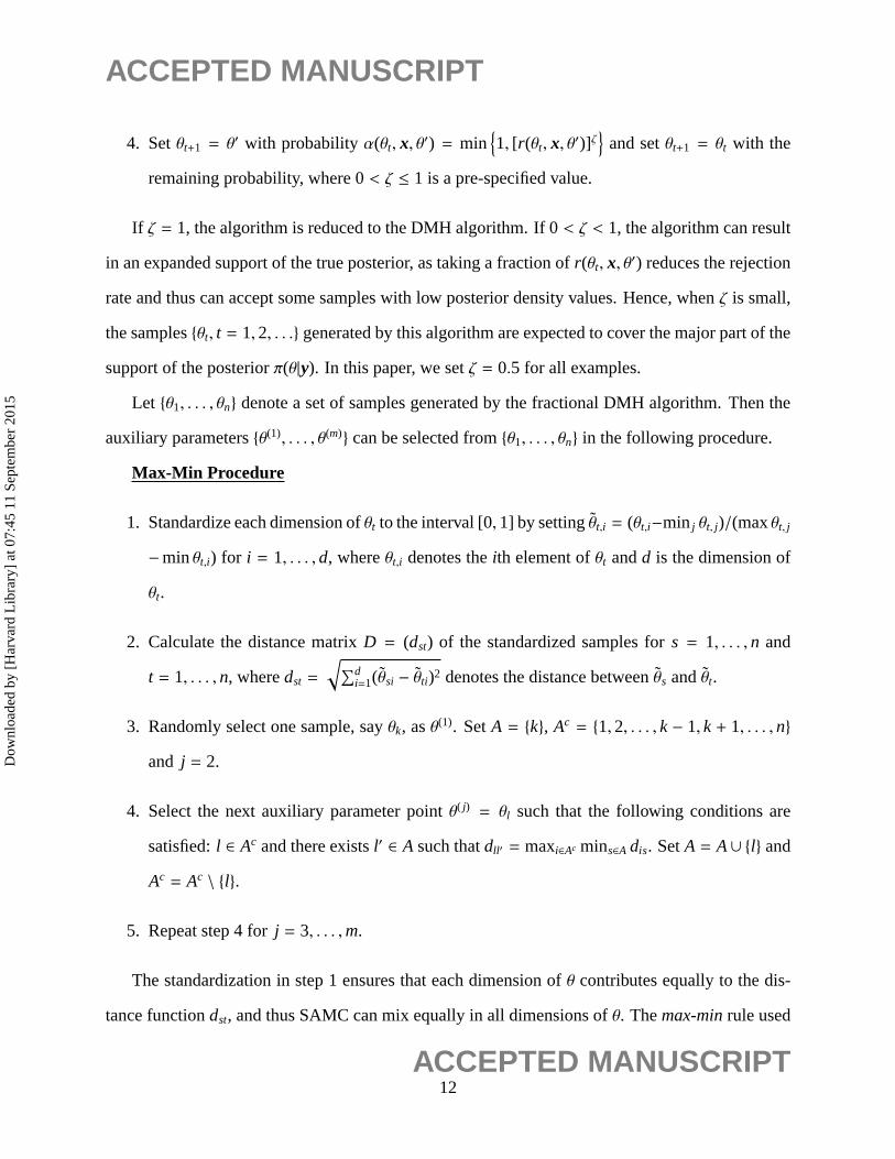
4. Setθt+1 = θ′ with probabilityα(θt, x, θ′) = min{1, [r(θt, x, θ′)]ζ
}and setθt+1 = θt with the
remaining probability, where 0< ζ ≤ 1 is a pre-specified value.
If ζ = 1, the algorithm is reduced to the DMH algorithm. If 0< ζ < 1, the algorithm can result
in an expanded support of the true posterior, as taking a fraction ofr(θt, x, θ′) reduces the rejection
rate and thus can accept some samples with low posterior density values. Hence, whenζ is small,
the samples{θt, t = 1,2, . . .} generated by this algorithm are expected to cover the major part of the
support of the posteriorπ(θ|y). In this paper, we setζ = 0.5 for all examples.
Let {θ1, . . . , θn} denote a set of samples generated by the fractional DMH algorithm. Then the
auxiliary parameters{θ(1), . . . , θ(m)} can be selected from{θ1, . . . , θn} in the following procedure.
Max-Min Procedur e
1. Standardize each dimension ofθt to the interval [0,1] by settingθt,i = (θt,i−minj θt, j)/(maxθt, j
−minθt,i) for i = 1, . . . , d, whereθt,i denotes theith element ofθt andd is the dimension of
θt.
2. Calculate the distance matrixD = (dst) of the standardized samples fors = 1, . . . , n and
t = 1, . . . , n, wheredst =
√∑di=1(θsi − θti)2 denotes the distance betweenθs andθt.
3. Randomly select one sample, sayθk, asθ(1). SetA = {k}, Ac = {1,2, . . . , k − 1, k + 1, . . . , n}
and j = 2.
4. Select the next auxiliary parameter pointθ( j) = θl such that the following conditions are
satisfied:l ∈ Ac and there existsl′ ∈ A such thatdll ′ = maxi∈Ac mins∈A dis. SetA = A∪ {l} and
Ac = Ac \ {l}.
5. Repeat step 4 forj = 3, . . . ,m.
The standardization in step 1 ensures that each dimension ofθ contributes equally to the dis-
tance functiondst, and thus SAMC can mix equally in all dimensions ofθ. Themax-minrule used
12ACCEPTED MANUSCRIPT
Dow
nloa
ded
by [
Har
vard
Lib
rary
] at
07:
45 1
1 Se
ptem
ber
2015

ACCEPTED MANUSCRIPT
in step 4 ensures that the selected samples{θ(1), . . . , θ(m)} and the full samples{θt, t = 1, . . . , n} have
about the same convex hull whenm is reasonably large, and thus{θ(1), . . . , θ(m)} are distributed over
the support of{θ1, . . . , θn}, i.e., condition (A0) is satisfied. Note that in the max-min rule,θ(2) is
always the furthest one fromθ(1) among the samples{θ1, . . . , θn}.
The numbermcan be determined by trial-and-error; that is, choosingmsuch that the auxiliary
chain can converge reasonably fast, e.g., within 103m ∼ 104m iterations. How to diagnose the
convergence of the auxiliary chain has been discussed at the end of Section 2.2. Besides the
auxiliary parameters and the gain factor sequence, the convergence of the auxiliary chain can
depend on the proposal distributions used in simulations. In our simulations, we usually setT2(∙|∙)
as the Gibbs sampler for updating auxiliary variables, and setT1(∙|∙) as the uniform distribution
over a pre-specified nearest neighbor for eachθ(i). In this paper, we setm = 100 and set the
neighboring sizem0 = 10 in all simulations. Different settings have been tried, such asm= 50 and
200 andm0 = 5, the results are similar. Since the auxiliary parameters are essentially generated
from the same posterior distribution, the neighboring distributionsf (y|θ(i))’s are always reasonably
overlapped. Note that they all share, at least approximately, the same sample—the observation
y. This ensures a smooth transition of the auxiliary chain between different auxiliary parameters.
More importantly, this property holds independently of the dimension ofθ. Hence, AEX can work
well for the problems for which the dimension ofθ is high. Here we note that when choosing
the values ofm andm0, the multimodality of the posteriorπ(θ|y) needs to be checked. If multiple
modes exist, special cares need to be taken in choosingm andm0 such that the resulting auxiliary
chain is irreducible.
Finally, we note that there can be many variations for the auxiliary parameter selection proce-
dure proposed above. For example, the fractional DMH algorithm can be replaced by any other
algorithm that can result in an expanded support of the target posteriorπ(θ|y), e.g., the approximate
Bayesian computation (ABC) algorithm (Beaumont et al., 2002). For the models for which the di-
mension ofθ is low, say, the spatial autologistic model studied in Section 4,{θ(1), . . . , θ(m)} can be
13ACCEPTED MANUSCRIPT
Dow
nloa
ded
by [
Har
vard
Lib
rary
] at
07:
45 1
1 Se
ptem
ber
2015

ACCEPTED MANUSCRIPT
set to some grid points around the MPLE ofθ. In themax-minprocedure, the standardization can
be replaced by a regular normalization procedure, i.e., settingθi = Σ−1/2n (θi − θn), whereθn andΣn
denote, respectively, the sample mean and covariance matrix of{θ1, . . . , θn}.
3 Convergence of the Adaptive Exchange Algorithm
As aforementioned, AEX falls into the class of adaptive MCMC algorithms. Since the transition
kernel of the exchange step may admit different stationary distributions for different iterations, the
convergence theory developed for conventional adaptive MCMC algorithms, see e.g., Roberts and
Rosenthal (2007) and Andrieu and Moulines (2006), is not applicable here. The ergodicity theory
developed by Fort et al. (2011) for adaptive MCMC allows to change stationary distributions at
different iterations and is indeed applicable to AEX. However, the strong law of large numbers es-
tablished therein requires some strong conditions that cannot be verified for AEX. For this reason,
we develop some theory for adaptive MCMC, including ergodicity and weak law of large numbers
(WLLN), which are applicable to AEX.
The remainder of this section is organized as follows. In Section 3.1, we prove two theorems,
ergodicity and weak law of large numbers, for general adaptive MCMC algorithms with changing
stationary distributions. In Section 3.2, we consider the weak convergence of auxiliary variables
drawn from the auxiliary chain. In Section 3.3, we establish the ergodicity and weak law of large
numbers for AEX.
3.1 Convergence of Adaptive MCMC with Changing Stationary Distribu-
tions
To facilitate our study, we first define, following Roberts and Rosenthal (2007), some notations for
adaptive Markov chains. Consider a state space (X,F ), whereF = B(X) denotes the Borel set
14ACCEPTED MANUSCRIPT
Dow
nloa
ded
by [
Har
vard
Lib
rary
] at
07:
45 1
1 Se
ptem
ber
2015
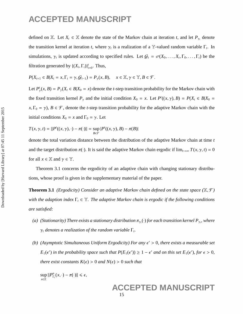
ACCEPTED MANUSCRIPT
defined onX. Let Xt ∈ X denote the state of the Markov chain at iterationt, and letPγt denote
the transition kernel at iterationt, whereγt is a realization of aY-valued random variableΓt. In
simulations,γt is updated according to specified rules. LetGt = σ(X0, . . . ,Xt, Γ0, . . . , Γt) be the
filtration generated by{(Xi , Γi)}ti=0. Thus,
P(Xt+1 ∈ B|Xt = x, Γt = γ,Gt−1) = Pγ(x, B), x ∈ X, γ ∈ Y, B ∈ F .
Let Ptγ(x, B) = Pγ(Xt ∈ B|X0 = x) denote thet-step transition probability for the Markov chain with
the fixed transition kernelPγ and the initial conditionX0 = x. Let Pt((x, γ), B) = P(Xt ∈ B|X0 =
x, Γ0 = γ), B ∈ F , denote thet-step transition probability for the adaptive Markov chain with the
initial conditionsX0 = x andΓ0 = γ. Let
T(x, γ, t) = ‖Pt((x, γ), ∙) − π(∙)‖ = supB∈F|Pt((x, γ), B) − π(B)|
denote the total variation distance between the distribution of the adaptive Markov chain at timet
and the target distributionπ(∙). It is said the adaptive Markov chain ergodic if limt→∞ T(x, γ, t) = 0
for all x ∈ X andγ ∈ Y.
Theorem 3.1 concerns the ergodicity of an adaptive chain with changing stationary distribu-
tions, whose proof is given in the supplementary material of the paper.
Theorem 3.1 (Ergodicity) Consider an adaptive Markov chain defined on the state space (X,F )
with the adaption indexΓt ∈ Y. The adaptive Markov chain is ergodic if the following conditions
are satisfied:
(a) (Stationarity) There exists a stationary distributionπγt(∙) for each transition kernel Pγt , where
γt denotes a realization of the random variableΓt.
(b) (Asymptotic Simultaneous Uniform Ergodicity) For anyε′ > 0, there exists a measurable set
E1(ε′) in the probability space such that P(E1(ε′)) ≥ 1− ε′ and on this set E1(ε′), for ε > 0,
there exist constants K(ε) > 0 and N(ε) > 0 such that
supx∈X‖Pn
Γt(x, ∙) − π(∙)‖ 6 ε,
15ACCEPTED MANUSCRIPT
Dow
nloa
ded
by [
Har
vard
Lib
rary
] at
07:
45 1
1 Se
ptem
ber
2015

ACCEPTED MANUSCRIPT
for all t > K(ε) and n> N(ε).
(c) (Diminishing Adaptation)lim t→0 Dt = 0 in probability, where
Dt = supx∈X‖PΓt+1(x, ∙) − PΓt(x, ∙)‖.
Theorem 3.1 is a slight extension of Theorem 1 of Roberts and Rosenthal (2007), where the
ergodicity is established for an adaptive Markov chain for which all transition kernels admit the
same stationary distribution and are simultaneously uniformly ergodic. Note that the conditions
(a) and (b) of Theorem 3.1 imply that on the setE1(ε′)
‖πΓt(∙) − π(∙)‖ = ‖πΓt(∙)PnΓt− π(∙)‖ ≤ sup
x‖Pn
Γt(x, ∙) − π(∙)‖ ≤ ε, (11)
for t > K(ε) andn > N(ε); that is, ast → ∞, πΓt(∙) converges toπ with probability greater than
1− ε′. Hence, in the limit case, Theorem 3.1 is reduced to the ergodicity theorem of Roberts and
Rosenthal (2007). The proof of Theorem 3.1 is also based on the coupling theory as in Roberts
and Rosenthal (2007).
We note that under a slightly weaker condition of (b), Fort et al. (2011) established the same
ergodicity result as Theorem 3.1. In this sense, Theorem 3.1 is redundant. Since part of its proof
will be used in the proof of the next theorem, it is presented in the supplementary material. Fort
et al. (2011) also established a strong law of large numbers for an adaptive Markov chain with
changing stationary distributions, but under rather strong conditions. For example, it requires an
explicit decreasing rate ofDt. However, figuring out the decreasing rate ofDt is very difficult, if not
impossible, for AEX. To address this issue, we develop the next theorem, whereDt can converge
to zero in probability at any rate. The proof of Theorem 3.2 can be found in the supplementary
material of the paper.
Theorem 3.2 (Weak Law of Large Numbers) Consider an adaptive Markov chain defined on the
state space (X,F ). Suppose that conditions (a), (b) and (c) of Theorem 3.1 hold. Let g(∙) be a
16ACCEPTED MANUSCRIPT
Dow
nloa
ded
by [
Har
vard
Lib
rary
] at
07:
45 1
1 Se
ptem
ber
2015

ACCEPTED MANUSCRIPT
bounded measurable function. Then
1n
n∑
t=1
g(Xt)→ π(g), in probability,
as n→ ∞, whereπ(g) =∫X
g(x)π(dx).
3.2 Weak Convergence of Auxiliary SAMC Samples
To study the weak convergence of the auxiliary samples collected via SAMC, we first describe a
general SAMC algorithm. Let
π(x) ∝ ψ(x), x ∈ X, (12)
denote the distribution that we want to draw samples from, whereX denotes the sample space
of π(x). Let E1, . . . ,Em denotem non-overlapping subregions, which form a partition ofX, i.e.,
X = ∪mi=1Ei andEi ∩Ej = ∅ for i , j. Let p= (p1, . . . , pm) denote the desired sampling frequencies
of respective subregions. Letwt = (w(1)t , . . . ,w(m)
t ) denote the vector of abundance factors attached
to the m subregions at iterationt, and letW denote the sample space ofwt. Let {Ks, s ≥ 0}
be a sequence of compact subsets ofW as defined in (7). LetX0 be a subset ofX, and let
T : X×W → X0×K0 be a truncation function which is measurable and maps a point inX×W to
a random point inX0×K0. Letσt denote the number of truncations performed until iterationt. Let
S denote the collection of the indices of the subregions from which a sample has been proposed;
that is,S contains the indices of all subregions which are known to be non-empty. The algorithm
starts with a random point drawn inX0 × K0 and then iterates in the following steps:
A General SAMC Sampler
(a) (Sampling) Simulate a samplex(t+1) by a single MH update with the target distribution given
by
πt(x) ∝m∑
i=1
ψ(x)
w(i)t
I (x ∈ Ei).
17ACCEPTED MANUSCRIPT
Dow
nloa
ded
by [
Har
vard
Lib
rary
] at
07:
45 1
1 Se
ptem
ber
2015
ACCEPTED MANUSCRIPT
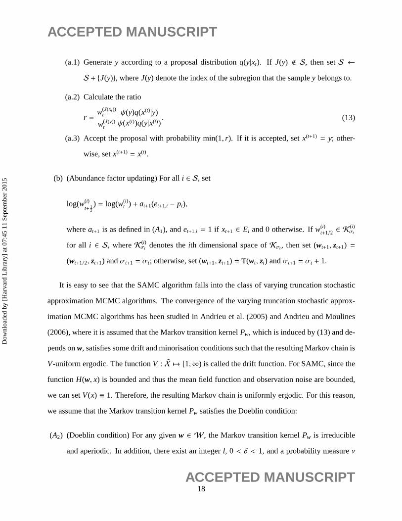
(a.1) Generatey according to a proposal distributionq(y|xt). If J(y) < S, then setS ←
S + {J(y)}, whereJ(y) denote the index of the subregion that the sampley belongs to.
(a.2) Calculate the ratio
r =w(J(xt))
t
w(J(y))t
ψ(y)q(x(t)|y)ψ(x(t))q(y|x(t))
. (13)
(a.3) Accept the proposal with probability min(1, r). If it is accepted, setx(t+1) = y; other-
wise, setx(t+1) = x(t).
(b) (Abundance factor updating) For alli ∈ S, set
log(w(i)
t+ 12
) = log(w(i)t ) + at+1(et+1,i − pi),
whereat+1 is as defined in (A1), andet+1,i = 1 if xt+1 ∈ Ei and 0 otherwise. Ifw(i)t+1/2 ∈ K
(i)σt
for all i ∈ S, whereK (i)σt denotes theith dimensional space ofKσt , then set (wt+1, zt+1) =
(wt+1/2, zt+1) andσt+1 = σt; otherwise, set (wt+1, zt+1) = T(wt, zt) andσt+1 = σt + 1.
It is easy to see that the SAMC algorithm falls into the class of varying truncation stochastic
approximation MCMC algorithms. The convergence of the varying truncation stochastic approx-
imation MCMC algorithms has been studied in Andrieu et al. (2005) and Andrieu and Moulines
(2006), where it is assumed that the Markov transition kernelPw, which is induced by (13) and de-
pends onw, satisfies some drift and minorisation conditions such that the resulting Markov chain is
V-uniform ergodic. The functionV : X 7→ [1,∞) is called the drift function. For SAMC, since the
functionH(w, x) is bounded and thus the mean field function and observation noise are bounded,
we can setV(x) ≡ 1. Therefore, the resulting Markov chain is uniformly ergodic. For this reason,
we assume that the Markov transition kernelPw satisfies the Doeblin condition:
(A2) (Doeblin condition) For any givenw ∈ W, the Markov transition kernelPw is irreducible
and aperiodic. In addition, there exist an integerl, 0 < δ < 1, and a probability measureν
18ACCEPTED MANUSCRIPT
Dow
nloa
ded
by [
Har
vard
Lib
rary
] at
07:
45 1
1 Se
ptem
ber
2015

ACCEPTED MANUSCRIPT
such that for any compact subsetK ⊂W,
infw∈K
Plw(x,A) ≥ δν(A), ∀x ∈ X, ∀A ∈ BX,
whereBX denotes the Borel set ofX; that is, the whole supportX is a small set for each
kernelPw, w ∈ K .
To verify (A2), one may assume thatX is compact,ψ(x) is bounded away from 0 and∞ on X,
and the proposal distributionq(y|x) satisfies thelocal positivecondition:
(Q) There existsδq > 0 andεq > 0 such that, for everyx ∈ X, |x− y| ≤ δq⇒ q(y|x) ≥ εq.
Then the condition (A2) holds following from Theorem 2.2 of Roberts and Tweedie (1996),
where it is shown that if the target distribution is bounded away from 0 and∞ on every compact set
of its supportX, then the MH chain with a proposal satisfying (Q) is irreducible and aperiodic, and
every non-empty compact set is asmallset. The proposals satisfying the local positive condition
can also be easily designed for both continuous and discrete systems. For continuous systems,
q(y|x) can be set to a random walk Gaussian proposal,y ∼ N(x, σ2Idx), whereσ2 can be calibrated
to have a desired acceptance rate, e.g., 0.2 ∼ 0.4. For discrete systems,q(y|x) can be set to
a discrete distribution defined on a neighborhood ofx. Besides the single-step MH move, the
multiple-step MH move, the Gibbs sampler, and the Metropolis-within-Gibbs sampler can also be
shown to satisfy (A2) under appropriate conditions, see e.g. Rosenthal (1995) and Liang (2009)
for the proofs. Note that to satisfy (A2), X is not necessarily compact. Rosenthal (1995) gave one
example for which the sample space is unbounded, yet the Markov chain is uniformly ergodic.
Under conditions (A1) and (A2), in a similar way to Liang et al. (2007), we can verify all
the conditions given in Andrieu et al. (2005) for the convergence of varying truncation stochastic
approximation MCMC algorithms. Hence, we claim that for SAMC, the number of truncations is
almost surely finite and for alli ∈ S,
log(w(i)t )→ C + log(ξi) − log(pi + ν), a.s., (14)
19ACCEPTED MANUSCRIPT
Dow
nloa
ded
by [
Har
vard
Lib
rary
] at
07:
45 1
1 Se
ptem
ber
2015

ACCEPTED MANUSCRIPT
as t → ∞, whereC denotes a constant,ξi =∫
Eiψ(x)dx, andν =
∑j∈{i:ξi=0} pj/(m− m0) andm0
is the cardinality of the set{i : ξi = 0}. The existence of empty subregions, i.e., the subregions
with ξi = 0, is due to an inappropriate partition of the sample space, but SAMC does allow for the
existence of empty subregions.
Further, we can show that a strong law of large numbers (SLLN) holds for SAMC: Ifψ(x) is
bounded away from 0 and∞ on X andX is compact, then for any bounded measurable function
G(x,w), whereG is Lipschitz continuous with respect tow , i.e. |G(x,w1)−G(x,w2)| ≤ L‖w1−w2‖
for someL > 0, we have
1n
n∑
t=1
G(Xt,wt)→ π∗(G), a.s., asn→ ∞, (15)
whereπ∗(∙) denotes the limit distribution ofπt(∙), andπ∗(G) denotes the expectation ofG(∙) with
respect toπ∗(∙). A proof of (15) is given in the supplementary material (Lemma A.1). A similar
result has been established in Atchade and Liu (2010) (Theorem 4.1) for a slightly different version
of SAMC, where the gain factor sequence is self-adapted. However, verification of their conditions
on stopping time is difficult.
For the auxiliary chain of AEX, we haveXt = (zt, ϑt), X = X×{θ(1), . . . , θ(m)} andEi = X×{θ(i)}.
In addition,ν, defined in (14), is equal to 0, as∫Xϕ(x, θ(i))dx > 0 for eachi. Let N denote the total
number of iterations of an AEX run. Then, it follows from (14) and (15) that
1N
N∑
t=1
m∑
i=1
{
w(i)tϕ(zt, θ
′)ϕ(zt, ϑt)
I (ϑt = θ(i))
}
→m∑
i=1
∫
X
κ(θ(i))pi
ϕ(z, θ′)ϕ(z, θ(i))
pi f (z|θ(i))dz= mκ(θ′), a.s., (16)
as N → ∞, provided thatX is compact and thus the ratioϕ(z, θ′)/ϕ(z, θ(i)) is bounded for all
z ∈ X. Note that ast → ∞, the marginal distribution ofzt converges to the mixture dis-
tribution p(z) =∑m
i=1 pi f (z|θ(i)). Since here we have implicitly assumed that the distributions
f (z|θ(i)), . . . , f (z|θ(m)) share the same sample spaceX, the condition (A0) is not necessary for, but
does benefit, the convergence of (16). Recall that the major role of the auxiliary parameters is to
be used for construction of a good trial distribution for drawing the auxiliary variables used in the
20ACCEPTED MANUSCRIPT
Dow
nloa
ded
by [
Har
vard
Lib
rary
] at
07:
45 1
1 Se
ptem
ber
2015
ACCEPTED MANUSCRIPT
target chain, and a good trial distribution can always improve the convergence of the importance
sampling procedure. Similarly, for any Borel setA ⊂ X, we have
(17)
Putting (16) and (17) together, we have, asN→ ∞,∑N
t=1
∑mi=1
{w(i)
tϕ(zt ,θ
′)ϕ(zt ,ϑt)
I (zt ∈ A & ϑt = θ(i))}
∑Nt=1
∑mi=1
{w(i)
tϕ(zt ,θ′)ϕ(zt ,ϑt)
I (ϑt = θ(i))} →
∫
Af (z|θ′)dz, a.s.,
which, by Lebesgue’s dominated convergence theorem, implies that
P(x ∈ A|θ′) = E[P(x ∈ A|z1, ϑ1,w1; . . . ; zN, ϑN,wN; θ′)
]→
∫
Af (z|θ′)dz, (18)
where (z1, ϑ1,w1; . . . ; zN, ϑN,wN) denotes a set of samples generated by the auxiliary chain, and
x denotes a sample resampled from (z1, ϑ1,w1; . . . ; zN, ϑN,wN). Furthermore, if the parameter
spaceΘ is compact and the functionϕ(z, θ) is upper semi-continuous inθ for all z ∈ X, then the
convergence in (18) is uniform overΘ. Refer to Ferguson (1996)(Theorem 16(a)) for a proof of
uniform strong law of large numbers. In summary, we have the following lemma:
Lemma 3.1 Assume that the conditions(A1) and (A2) are satisfied, andX is compact. ϕ(x, θ)
is bounded away from 0 and∞ onX × Θ. Let {z1, ϑ1,w1; . . . ; zN, ϑN,wN} denote a set of samples
generated by SAMC in an AEX run, and letx1, . . . , xn be distinct samples inzt. Resample a random
variable/vector X from{z1, ϑ1,w1; . . . ; zN, ϑN,wN} such that
P(X = xk|θ′) =
∑Nt=1
∑mi=1
{w(i)
tϕ(zt ,θ
′)ϕ(zt ,ϑt)
I (zt = xk & ϑt = θ(i))}
∑Nt=1
∑mi=1
{w(i)
tϕ(zt ,θ′)ϕ(zt ,ϑt)
I (ϑt = θ(i))} , k = 1, . . . , n,
then the distribution of X converges to f(∙|θ′) almost surely as N→ ∞. Furthermore, ifΘ is
compact and the unnormalized density functionϕ(z, θ) is upper semi-continuous inθ for all z ∈ X,
then the convergence is uniform overΘ.
As aforementioned, sincef (z|θ(i))’s share the same sample spaceX, the condition (A0) is not
necessary for, but does benefit, the convergence stated in the lemma. For the efficiency of the
algorithm, (A0) is generally required to be satisfied.
21ACCEPTED MANUSCRIPT
Dow
nloa
ded
by [
Har
vard
Lib
rary
] at
07:
45 1
1 Se
ptem
ber
2015

ACCEPTED MANUSCRIPT
3.3 Convergence of AEX
To study the convergence of AEX, we first note that{θt} forms an adaptive Markov chain with the
transition kernel given by
Pl(θ, dθ′) =
∫
Xα(θ, x, θ′)q(dθ′|θ)νl(dx|θ′) + δθ(dθ′)
[1−
∫
Θ×Xα(θ, x, ϑ′)q(dϑ′|θ)νl(dx|ϑ′)
], (19)
whereα(θ, x, θ′) is defined in (10),l denotes the cardinality of the set of auxiliary variables col-
lected from the auxiliary Markov chain, i.e.,l = |Sl |, andνl(x|θ′) denotes the true distribution ofx
resampled fromSl. For mathematical simplicity, we assume that the parameter spaceΘ (of θ) and
the sample spaceX (of x) are both compact. Although this makes our theory a little restrictive, it is
quite common in the study of adaptive Markov chain theory, say e.g., Haario et al. (2001). Under
this assumption, we have the following lemma, whose proof can be found in the supplementary
material.
Lemma 3.2 Assume that conditions(A1) and (A2) are satisfied, bothX andΘ are compact, and
the unnormalized density functionϕ(x, θ) is continuously differentiable inθ for all x ∈ X and
bounded away from 0 and∞ onX × Θ. Furthermore, assumeπ(θ) and q(θ′|θ) are continuously
differentiable inθ andθ′ as well. DefineDl = supθ∈Θ ‖Pl(θ, ∙) − P(θ, ∙)‖, where P(θ, ∙), as defined in
(5), denotes the transition kernel of the exchange algorithm with perfect auxiliary variables. Then
Dl → 0 almost surely as l→ ∞.
It is known thatP(θ, dθ′) can induce a Markov chain which is irreducible, aperiodic and admits
π(θ|y) as the invariant distribution, provided an appropriate proposalq(∙|∙) been used therein. Define
βl(θ, x, θ′) =νl(x|θ′)νl(x|θ)
f (x|θ)f (x|θ′)
, and
r(θ, x, θ′) =π(θ′) f (y|θ′)π(θ) f (y|θ)
q(θ|θ′)q(θ′|θ)
f (x|θ)f (x|θ′)
, rv(θ, x, θ′) =π(θ′) f (y|θ′)π(θ) f (y|θ)
q(θ|θ′)q(θ′|θ)
νl(x|θ)νl(x|θ′)
.
Then it is easy to see that
r(θ, x, θ′) = βl(θ, x, θ′)rv(θ, x, θ′),
22ACCEPTED MANUSCRIPT
Dow
nloa
ded
by [
Har
vard
Lib
rary
] at
07:
45 1
1 Se
ptem
ber
2015

ACCEPTED MANUSCRIPT
and the Markov chain defined by the acceptance rule min{1, rv(θ, x, θ′)} is irreducible, aperiodic
and admits the invariant distributionπ(θ|y), provided an appropriate proposalq(∙, ∙) has been used
therein. To ensure the convergence of the Markov chain,νl(x|θ) is not necessarily to have a support
as large asX. In fact, its support can be only a subset ofX. Let Pv(θ, dθ′) denote the transitional
kernel of the Markov chain induced by the acceptance rule min{1, rv(θ, x, θ′)}. Lemma 3.3 shows
thatPl(θ, dθ′), defined in (19), is also irreducible and aperiodic and admits an invariant distribution.
This is done by showing that the accessible sets ofPv are included in those ofPl. The details are
given in the supplementary material.
Lemma 3.3 Assume (i) the conditions of Lemma 3.2 hold and (ii) P is irreducible and aperiodic
and admits an invariant distribution. ThenPl, defined in (19), is irreducible and aperiodic, and
hence there exists a stationary distributionπl(θ|x) such that for anyθ0 ∈ Θ,
limk→∞‖Pk
l (θ0, ∙) − πl(∙|y)‖ = 0.
If the proposal q(∙, ∙) satisfies the local positive condition(Q), then the ergodicity is uniform over
Θ.
Lemma 3.4 concerns the simultaneous uniform ergodicity of the kernelPl ’s, whose proof can
be found in the supplementary material.
Lemma 3.4 Assume the conditions of Lemma 3.3 hold. If the proposal q(∙, ∙) satisfies the local
positive condition, then for any e> 0 there exits a measurable set E0 in the probability space such
that P(E0) > 1− e and on this set E0, for anyε > 0, there exist L(ε) ∈ N and K(ε) ∈ N such that
for any l> L(ε) and k> K(ε),
‖Pkl (θ0, ∙) − π(∙|y)‖ ≤ ε, for all θ0 ∈ Θ. (20)
DefineDl = supθ∈Θ ‖Pl+1(θ, ∙)−Pl(θ, ∙)‖. SinceDl ≤ supθ∈Θ ‖Pl+1(θ, ∙)−P(θ, ∙)‖+supθ∈Θ ‖Pl(θ, ∙)−
P(θ, ∙)‖, by Lemma 3.2, we have liml→∞ Dl = 0 almost surely. That is,Pl satisfies the diminishing
23ACCEPTED MANUSCRIPT
Dow
nloa
ded
by [
Har
vard
Lib
rary
] at
07:
45 1
1 Se
ptem
ber
2015
ACCEPTED MANUSCRIPT
adaptation condition of Theorem 3.1. Putting this together with Lemmas 3.3 and 3.4, we have the
following theorem, which states that AEX is ergodic and the weak law of large numbers holds for
the sample path average.
Theorem 3.3 (Ergodicity and WLLN) Assume the conditions of Lemma 3.3 hold. If the proposal
q(∙, ∙) satisfies the local positive condition and the unnormalized density functionϕ(x, θ) is upper
semi-continuous inθ for all x ∈ X, then the adaptive exchange algorithm is ergodic and for any
bounded measurable function g,
1n
n∑
i=1
g(θi)→ π(g|y), in probability,
as n→ ∞, whereπ(g|y) =∫Θ
g(θ)π(θ|y)dθ.
4 Spatial Autologistic Model
The spatial autologistic model (Besag, 1974) has been widely used in spatial data analysis (e.g.,
Preisler, 1993; Sherman et al., 2006). Lety = {yi : i ∈ D} denote the observed binary data, where
yi is called a spin andD is the set of indices of the spins. Let|D| denote the total number of spins
in D, and letn(i) denote the set of neighbors of spini. The likelihood function of the model is
given by
f (y|α, β) =1
κ(α, β)exp
α∑
i∈D
yi +β
2
∑
i∈D
yi
∑
j∈n(i)
yj
, (α, β) ∈ Θ, (21)
where the parameterα determines the overall proportion ofyi = ±1, the parameterβ determines
the intensity of interaction betweenyi and its neighbors, andκ(α, β) is the intractable normalizing
constant defined by
κ(α, β) =∑
for all possible yexp
α∑
i∈D
yi +β
2
∑
i∈D
yi
∑
j∈n(i)
yj
. (22)
24ACCEPTED MANUSCRIPT
Dow
nloa
ded
by [
Har
vard
Lib
rary
] at
07:
45 1
1 Se
ptem
ber
2015

ACCEPTED MANUSCRIPT
An exact evaluation ofκ(α, β) is prohibited even for a moderate system. To conduct a Bayesian
analysis for the model, a uniform prior on
(α, β) ∈ Θ = [−1,1] × [0,1],
is assumed for the parameters, which restrictsΘ to be a compact set. SinceD is finite, the sample
spaceX (of y) is also finite.
4.1 U.S. Cancer Mortality Data
United States cancer mortality maps have been compiled by Riggan et al. (1987) for investigating
the possible association of cancer with unusual demographic, environmental, and industrial char-
acteristics, or employment patterns. Figure 1(a) shows the mortality map for cancer of the liver and
gallbladder (including bile ducts) cancers in white males during the decade 1950-1959, which indi-
cates some apparent geographic clustering. See Sherman et al. (2006) for more descriptions of the
data. Following Sherman et al. (2006), we modeled the data with a spatial autologistic model. The
total number of spins is|D| = 2293. A free boundary condition is assumed for the model, under
which the boundary points have fewer neighboring points than the interior points. This assumption
is natural to this dataset, as the lattice has an irregular shape.
The AEX algorithm was first applied to this example. It was run for 10 times indepen-
dently. Each run consisted of three stages. The first stage was to choose the auxiliary parameters
{θ(1), . . . , θ(m)}. For this purpose, the fractional DMH algorithm was run forN1 = 5500 iterations
and 5000 samples ofθ were collected after a burn-in period of 500 iterations, and thenm = 100
auxiliary parameters were selected from the 5000 collected samples using themax-minprocedure.
The second stage was to build up an initial database of auxiliary variables. In this stage, only the
auxiliary chain was run. The auxiliary chain started with the observed datay andw0 = (1, . . . , 1),
and consisted ofN2 = 1.1 × 10⁶ iterations. The first 105 iterations were discarded for the burn-
25ACCEPTED MANUSCRIPT
Dow
nloa
ded
by [
Har
vard
Lib
rary
] at
07:
45 1
1 Se
ptem
ber
2015

ACCEPTED MANUSCRIPT
in process, and then a database of 50000 auxiliary variables was collected from the remainder
of the run at an equal time space ofs0 = 20 iterations. In the simulations, we setX0 = X and
Ki = [0,10100+10i] for i = 0,1,2, . . .. In the third stage, the auxiliary chain and the target chain
were run simultaneously. The auxiliary chain was run forN3 = 4× 10⁵ iterations and the samples
generated by it were continuously collected (at a time space ofs0 = 20 iterations) and added into
the database, and the target chain was run for 20,000 iterations. The target chain started with the
average of theθ samples collected from the fractional DMH run, and was run for one iteration
once a new auxiliary variable was added to the database. The CPU time for the whole run is 107s,
which is measured on a single core of IntelR© XeonR© CPU E5-2690(2.90Ghz) (the same computer
was used for all simulations of this paper). The samples generated in the target chain were used
for Bayesian inference of the model. For both the fractional DMH chain and the target chain, a
Gaussian random walk proposal distribution with the covariance matrix 0.032I2 was used, where
I2 denotes the 2-by-2 identity matrix. The overall acceptance rate of the target chain is 0.21, and
that of the fractional DMH chain is 0.33. For the auxiliary chain, the proposal distributionT2(∙|∙)
was set to a single cycle of Gibbs updates.
Figure 2(a) shows the scatter plot of the fractional DMH samples and the selected auxiliary
parameters. The scatter plot of the selected auxiliary parameters is also shown in Figure 2(b).
As expected, the selected auxiliary parameters are distributed over the space of fractional DMH
samples, and the convex hulls formed by them are about the same. Figure 2(c) shows the histogram
of the 100 auxiliary parameters achieved by the auxiliary chain in a run with the uniform desired
sampling distribution. The flatness of the histogram implies that the auxiliary chain has converged.
A MCMC convergence diagnosis based on Gelman-Rubin’s shrink factor (Gelman and Rubin,
1992), as shown in Figure 3, indicates that for this example AEX can converge very fast, usually
within a few hundred iterations. Figure 3 was generated using the R packagecoda (Plummer
et al., 2012) based on ten independent runs of AEX. As for conventional MCMC algorithms, the
samples generated in the early stage of these runs can be discarded for the burn-in process. Table
26ACCEPTED MANUSCRIPT
Dow
nloa
ded
by [
Har
vard
Lib
rary
] at
07:
45 1
1 Se
ptem
ber
2015
ACCEPTED MANUSCRIPT
1 summarizes the parameter estimation results for the model based on the ten independent runs.
To assess the validity of the AEX algorithm, the exchange algorithm was applied to this ex-
ample with the same proposal distribution as used in the target chain of AEX. As previously men-
tioned, the exchange algorithm is an auxiliary variable MCMC algorithm that requires a perfect
sampler for generating auxiliary variables, and it can sample correctly from the posterior distribu-
tion when the number of iterations is large. Hence, the estimates produced by the exchange algo-
rithm can be used as the test standard for assessing the performance of AEX. For this example, the
auxiliary variables were generated using the summary state algorithm (Childs et al., 2001), which
is suitable for high-dimensional binary spaces. The exchange algorithm was run for 10 times inde-
pendently. Each run consisted of 20,500 iterations, where the first 500 iterations were discarded for
the burn-in process, and the remaining 20,000 iterations were used for estimation ofθ. Therefore,
in each run, the exchange and AEX algorithm produced the same number of samples. Each run of
the exchange algorithm costs about 106s CPU time, and the overall acceptance rate was 0.21 which
indicates the algorithm has been implemented efficiently. The numerical results are summarized
in Table 1. The estimates produced by the AEX and exchange algorithms are also very close to
those reported in the literature. Liang (2007) analyzed these data using a contour Monte Carlo
method and produced the estimate (-0.3008, 0.1231). The contour Monte Carlo method approxi-
mates the normalizing constant function on a given region and then estimates the parameters based
on the approximated normalizing constant function. As reported by Liang (2007), this algorithm
took several hours of CPU time to approximate the normalizing constant function. Sherman et al.
(2006) analyzed the data using the MCMLE method (Geyer and Thompson, 1992), and obtained
the estimate (-0.304, 0.117), which is different from other Bayesian estimates. This may reflect the
difference between the posterior mean and posterior mode.
For a thorough comparison, we have also applied the DMH and MCMH algorithm to this
example. As aforementioned, the DMH sampler is the same with the exchange algorithm except
that it draws the auxiliary variablex at each iteration through a finite run of the MH algorithm
27ACCEPTED MANUSCRIPT
Dow
nloa
ded
by [
Har
vard
Lib
rary
] at
07:
45 1
1 Se
ptem
ber
2015

ACCEPTED MANUSCRIPT
initialized at the observationy. In our implementation, we set the length of the finite MH run to be
K = 50. DMH was run for 10 times. Each run consisted of 20,500 iterations and cost about 142s,
where the samples generated in the last 20,000 iterations were used for parameter estimation. The
results are summarized in Table 1.
The MCMH algorithm works in a different idea from DMH. It is not to cancel the unknown
normalizing constant ratio using auxiliary variables, but to approximate the normalizing constant
ratio using auxiliary variables. Letθt denote the sample ofθ drawn at iterationt, and letx(t)1 , . . . , x
(t)K
denote the auxiliary samples simulated from the distributionf (x|θt). One iteration of the MCMH
algorithm consists of the following steps:
Monte Carlo MH algorithm:
1. Drawθ′ from a proposal distributionq(θ′|θt).
2. Estimate the normalizing constant ratioκ(θ′)/κ(θt) by R(θt, x1, . . . , xK , θ′) = 1
K
∑Ki=1
ψ(xi ,θ′)
ψ(xi ,θt),
and then calculate the ratio
r(θt, x1, . . . , xK , θ′) =
1
R(θt, x1, . . . , xK , θ′)
ψ(y, θ′)π(θ′)q(θt|θ′)ψ(y, θt)π(θt)q(θ′|θt)
.
3. Setθt+1 = θ′ with probability min{1, r(θt, x1, . . . , xK , θ′)} and setθt+1 = θt with the remaining
probability.
4. If the proposal is rejected in step 3, setx(t+1)i = x(t)
i for i = 1, . . . ,K. Otherwise, simulate
samplesx(t+1)1 , . . . , x(t+1)
K from f (x|θt+1) using the MH algorithm.
We note that the MCMH algorithm, an early version of this algorithm is presented in the book
by Liang et al. (2010), is similar to the marginal PMCMC algorithm suggested by Everitt (2012).
The MCMH algorithm is to use auxiliary variables to approximate the unknown normalizing con-
stant ratio, while the marginal PMCMC algorithm, based on the work by Andrieu et al. (2010), is
to use sequential Monte Carlo samples to approximate the unknown normalizing constant.
28ACCEPTED MANUSCRIPT
Dow
nloa
ded
by [
Har
vard
Lib
rary
] at
07:
45 1
1 Se
ptem
ber
2015

ACCEPTED MANUSCRIPT
In our implementation of MCMH, we setK = 100 and the proposalq(∙|∙) to be a Gaussian
random walk with the covariance matrix 0.032I2. The algorithm was run for 10 times indepen-
dently. Each run consisted of 20500 iterations, where the first 500 iterations were for the burn-in
process, and cost about 143s CPU time. The overall acceptance rate was about 0.35. The results
are summarized in Table 1.
Table 1 shows that all the algorithms, AEX, DMH, MCMH and exchange, work well for this
example. By treating the estimates of the exchange algorithm as the testing standard, it is easy to
see that the estimates resulted from all the other three algorithms are unbiased. This is because
the underlying system of this example dataset is only weakly dependent, and thus independent
auxiliary samples can be easily drawn at each iteration by running a short Markov chain. In terms of
efficiency, MCMH is the best among the three approximate MCMC algorithms. This is reasonable,
as in MCMH the auxiliary sample are only drawn when a new sample ofθ is accepted and all the
auxiliary samples are used in simulating new samples ofθ. For this example, MCMH has about
the same efficiency as the exchange algorithm after taking account of their CPU times and standard
deviations of the estimates. Compared to MCMH, AEX and DMH are less efficient in the use of
auxiliary samples. AEX makes use of only a small proportion of the auxiliary samples and discards
all the others. DMH is similar; it uses only the last sample generated by the short Markov chain at
each iteration.
In Section 4.2, we present one example for which the underlying system is strongly dependent.
Since, for such a system, independent auxiliary samples are difficult to draw with a short run of
Markov chain, AEX outperforms the DMH and MCMH algorithms.
4.2 A Simulation Study
To assess the performance of the AEX algorithm for strongly dependent systems, we simulated
one U.S. cancer mortality dataset using the summary state algorithm withα = 0 andβ = 0.45.
29ACCEPTED MANUSCRIPT
Dow
nloa
ded
by [
Har
vard
Lib
rary
] at
07:
45 1
1 Se
ptem
ber
2015
ACCEPTED MANUSCRIPT
Since the lattice is irregular, the free boundary condition was again assumed in the simulation.
Note that under the settingα = 0, the autologistic model is reduced to the Ising model. Hence, the
underlying system for this simulated dataset is strongly dependent by noting that the interaction
parameterβ is greater than the critical value (≈ 0.44) of the Ising model.
AEX was first applied to this example. It was run as for the last example except that the
simulations in the second and third stages have been lengthened. For this example, we setN2 =
6 × 10⁶, s0 = 50, andN3 = 106, where the first 106 iterations in the second stage were used for
the burn-in process. AEX was run for 10 times independently, and each run costs about 327s. The
numerical results are summarized in Table 2.
For comparison, we have also applied the exchange, DMH and MCMH to this example. The
exchange algorithm was run for 10 times. Each run consisted of 1200 iterations, where the first
200 iterations were discarded for the burn-in process and the samples generated in the remaining
iterations were used for parameter estimation. The proposal distribution is the same as that used
for the last example. For the exchange algorithm, due to its difficulty in generating perfect samples,
the CPU time of each run can be very long although consisting of only 1200 iterations. In addition,
the CPU times of different runs can be much different. Childs et al. (2001) studied the behavior of
the perfect sampler for the Ising model. They fitted an exponential law for the convergence time,
and reported that the perfect sampler may not work well when the value ofβ is close to the critical
value (≈ 0.44). Their finding is consistent with our results reported in Table 2.
In applying DMH to this example, we tried different values ofK, K = 10, 100, 500 and 1000,
to assess the effect of mixing of the short Markov chain on parameter estimation. For MCMH, we
have also tried the same settings ofK. Both DMH and MCMH were run for 10 times independently,
and each run consisted of 20,500 iterations with the first 500 iterations discarded for the burn-in
process. The results are summarized in Table 2. As shown in Table 2, for the same value ofK,
MCMH generally costs less CPU times than DMH, as MCMH only generates auxiliary variables
when a new value ofθ is accepted, while in DMH this needs to be done at each iteration. Table 2
30ACCEPTED MANUSCRIPT
Dow
nloa
ded
by [
Har
vard
Lib
rary
] at
07:
45 1
1 Se
ptem
ber
2015
ACCEPTED MANUSCRIPT
shows that both the DMH and MCMH estimates ofβ have a trend of decreasing toward the true
value 0.45. However, even withK = 1000, at which both DMH and MCMH cost more CPU times
than AEX, their estimates are still far from the true value. In contrast, even AEX costs much less
CPU time than these two algorithms (withK = 1000), its estimate ofβ is much closer to the true
value and also the estimate of the exchange algorithm.
To have a fully exploration for the performance of different algorithms, we show in Figure 4
the box-plots of theβ estimates resulted from 10 independent runs by the above four algorithms.
It shows again the superiority of AEX for this example: AEX can work well for the problems for
which the underlying system is strongly dependent, while DMH and MCMH cannot.
5 Autonormal Model
5.1 Autonormal Model
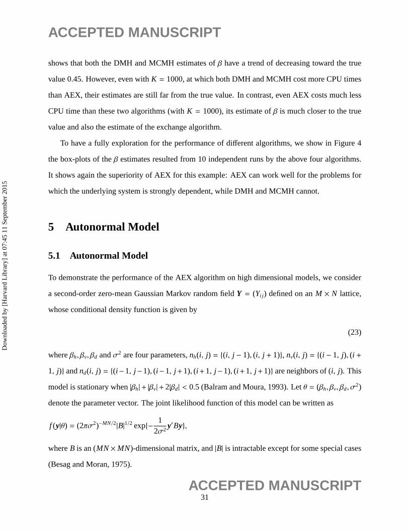
To demonstrate the performance of the AEX algorithm on high dimensional models, we consider
a second-order zero-mean Gaussian Markov random fieldY = (Yi j ) defined on anM × N lattice,
whose conditional density function is given by
(23)
whereβh, βv, βd andσ2 are four parameters,nh(i, j) = {(i, j − 1), (i, j + 1)}, nv(i, j) = {(i − 1, j), (i +
1, j)} andnd(i, j) = {(i −1, j −1), (i −1, j +1), (i +1, j −1), (i +1, j +1)} are neighbors of (i, j). This
model is stationary when|βh|+ |βv|+2|βd| < 0.5 (Balram and Moura, 1993). Letθ = (βh, βv, βd, σ2)
denote the parameter vector. The joint likelihood function of this model can be written as
f (y|θ) = (2πσ2)−MN/2|B|1/2 exp{−1
2σ2y′By},
whereB is an (MN×MN)-dimensional matrix, and|B| is intractable except for some special cases
(Besag and Moran, 1975).
31ACCEPTED MANUSCRIPT
Dow
nloa
ded
by [
Har
vard
Lib
rary
] at
07:
45 1
1 Se
ptem
ber
2015

ACCEPTED MANUSCRIPT
To conduct a Bayesian analysis for the model, we assume the following priors:
π(β) ∝ I (|βh| + |βv| + 2|βd| < 0.5), π(σ2) ∝1σ2, (24)
which I (∙) is the indicator function. Under the free boundary condition for which the boundary
pixels have fewer neighbors, we have the following posterior distribution
π(β, σ2|y) ∝ (σ2)−MN2 −1|B|1/2 exp
{−
MN2σ2
(Sy−2βhYh−2βvYv−2βdYd
)}I (|βh|+ |βv|+2|βd| < 0.5),(25)
where
Althoughσ2 can be integrated out from the posterior, we do not suggest to do so. Working on the
joint posterior will ease the generation of auxiliary variables in AEX.
5.2 Wheat Yield Data
The wheat yield data was collected on a 20× 25 rectangular lattice (Table 6.1, Andrews and
Herzberg, 1985). The data was shown in Figure 5(a), which indicates positive correlation between
neighboring observations. This data has been analyzed by a number of authors, e.g., Besag (1974),
Huang and Ogata (1999), and Gu and Zhu (2001). Following the previous authors, we subtracted
the mean from the data and then fitted them by the autonormal model. In our analysis, the free
boundary condition is assumed. This is natural, as the lattice for the real data is often irregular.
The AEX algorithm was applied to this example in a similar way to the cancer mortality data
example. The algorithm was run for 10 times independently. Each run consisted of three stages,
and their settings are the same as the runs for the simulated cancer mortality data except for the
proposal distributions. For both the fractional DMH chain and the target chain, a Gaussian random
walk proposal with the covariance matrix 0.012I4 was used, whereI4 denotes the 4-by-4 identity
matrix. For the auxiliary chain, the proposalT2(∙|∙) was set to a single cycle of Gibbs updates:
yi j |y(u,v)∈n(i, j) ∼ N
βht
∑
(u,v)∈nh(i, j)
yuv + βvt
∑
(u,v)∈nv(i, j)
yuv + βdt
∑
(u,v)∈nd(i, j)
yuv, σ2t
,
32ACCEPTED MANUSCRIPT
Dow
nloa
ded
by [
Har
vard
Lib
rary
] at
07:
45 1
1 Se
ptem
ber
2015

ACCEPTED MANUSCRIPT
for i = 1, . . . ,M and j = 1, . . . ,N, where (βht, βvt, βdt, σ2t ) denotes the value ofθ at iterationt. Each
run of AEX cost about 402s. Figure 5(b) shows the histogram of the 100 auxiliary parameters
achieved by the auxiliary chain at the end of the second stage. It indicates that the auxiliary
chain can mix very well for different auxiliary parameters. The parameter estimation results are
summarized in Table 3.
For this example, the exchange algorithm is not applicable, as the perfect sampler is not avail-
able for the autonormal model. However, under the free boundary condition, the log-likelihood
function of the model admits the following analytic form (Balram and Moura, 1993):
(26)
whereSy, Yh, Yv and Yd are as defined in (25). The Bayesian inference for the model is then
standard, with the priors as specified in (24). For comparison, the MH algorithm has been applied
to simulate from the resulting analytic posterior distribution. It was run for 10 times with each run
consisting of 20,500 iterations, where the first 500 iterations were discarded for the burn-in process.
The proposal distribution adopted here was a Gaussian random walk with the same covariance
matrix as that used in AEX. The overall acceptance rate is about 0.45. The resulting parameter
estimates, the so-called true Bayes estimates, are summarized in Table 3. The comparison indicates
that AEX works well for this example.
This example implies that AEX can work well for reasonably high dimensional problems. As
aforementioned, the key to the success of AEX is to be able to generate auxiliary variables at a
set of auxiliary parameters that cover the support of the true posterior. In AEX, all the auxiliary
parameters are selected from the samples generated by the fractional DMH algorithm which can
result in an expanded support of the true posterior. This, together with themax-minprocedure,
ensures that the selected auxiliary parameters are able to cover the support of the true posterior.
Since the auxiliary parameters are essentially generated from the same posterior distribution, the
neighboring distributionsf (x|θ(i))’s are reasonably overlapped by noting that they all share, at least,
33ACCEPTED MANUSCRIPT
Dow
nloa
ded
by [
Har
vard
Lib
rary
] at
07:
45 1
1 Se
ptem
ber
2015
ACCEPTED MANUSCRIPT
the same sample—the observationy. This ensures a smooth transition of the auxiliary chain be-
tween different auxiliary parameters and thus the success of AEX. More importantly, this property
of AEX holds independent of the dimension ofθ. For the wheat yield data example, the overall
acceptance rate for the transitions between different auxiliary parameters is about 0.25.
6 Conclusion
We have proposed a new algorithm, the adaptive exchange algorithm or AEX in short, for sam-
pling from distributions with intractable normalizing constants. The new algorithm can be viewed
as a MCMC extension of the exchange algorithm, which generates auxiliary variables via an im-
portance sampling procedure from a Markov chain running in parallel. The convergence of the
new algorithm, including ergodicity and weak law of large numbers, has been established under
mild conditions. Compared to the exchange algorithm, the new algorithm removes the require-
ment of perfect sampling, and thus can be applied to many models for which perfect sampling is
not available or very expensive. The new algorithm has been tested on the spatial autologistic and
autonormal models. The numerical results indicate that the new algorithm can outperform other
approximate MCMC algorithms, such as the DMH and MCMH algorithms, for strongly dependent
systems.
We have also applied the AEX algorithm to some more challenging problems, such as expo-
nential random graph models for social networks. Our numerical results indicate that the AEX
algorithm can outperform other approximate algorithms for large social networks. When the net-
work is large, generating independent auxiliary networks is often difficult with a short Markov
chain. Due to the space limit, these results will be reported elsewhere.
Our implementation of AEX is plain. Its efficiency can be improved in various respects. For
example, in the current implementation, the auxiliary parameters are selected using amax-min
procedure. In the future, a self-learning process may be introduced to the auxiliary Markov chain
34ACCEPTED MANUSCRIPT
Dow
nloa
ded
by [
Har
vard
Lib
rary
] at
07:
45 1
1 Se
ptem
ber
2015

ACCEPTED MANUSCRIPT
toward an optimal selection of the auxiliary parameters. To improve the mixing of the target chain,
a population-based MCMC algorithm may be used, e.g., adaptive direction sampling, parallel tem-
pering or evolutionary Monte Carlo. We note that AEX can slow down with iterations, because it
needs to resample from an increasingly large database.
Finally, we would like to compare, mainly conceptually, the AEX algorithm and the Russian
Roulette sampling algorithm (Lyne et al., 2014). The latter is developed based on the pseudo-
marginal MCMC approach of Andrieu and Roberts (2009), which requires an unbiased indepen-
dent estimate of the intractable normalizing constant at each iteration. Hence, the algorithm can be
extremely slow. For an Ising model example of 100 spins, where the normalizing constant is esti-
mated using annealing importance sampling (Neal, 1998) at each iteration, the algorithm costs over
100 CPU minutes (on the same computer as used by AEX for the previous examples) for running
1000 iterations under the authors’ default setting. The AEX algorithm also relies on the estimates
of intractable normalizing constants, but only on a number of pre-specified points. Moreover, the
estimates are obtained in an online manner and can be improved with iterations. Hence, the AEX
algorithm can be much more efficient than the Russian Roulette sampling algorithm. This is evi-
denced by Table 2, where it is reported that AEX cost only 5.5 CPU minutes for running 20,000
iterations for a two-parameter spatial autologistic model of 2293 spins.
For large-scale problems that the datasetY consists of a large number of observations, the
difficulty arises from evaluation of the likelihood function. For the Russian Roulette sampling
algorithm, its theory allows it to work with an unbiased estimate of the likelihood function. This is
a strength of the Russian Roulette sampling algorithm, although achieving such an estimate at each
iteration is again difficult. Sophisticated computational techniques, such as parallel computing and
subsampling, may be needed there. For the AEX algorithm, to tackle this difficulty, it can be used
with a split-and-merge strategy; that is, one can split the big dataset into many small subsets (e.g.,
through subsampling), perform AEX simulations for each subset data independently, and then
combine the simulation results from each subset data to get the entire data-based inference. For
35ACCEPTED MANUSCRIPT
Dow
nloa
ded
by [
Har
vard
Lib
rary
] at
07:
45 1
1 Se
ptem
ber
2015

ACCEPTED MANUSCRIPT
example, if we are merely interested in parameter estimation, the estimates from different subset
data can be combined using a meta-analysis method (see e.g., Chang, 2011). If we are interested
in posterior samples, the combination might be done via a random set intersection method, which
is, to some extent, related to Dempster’s rule of recombination operation in the Dempster-Shafer
theory of belief functions (see e.g., Martin et al., 2010). This method has been explored in Lin
(2014) for the case that the subset data are mutually independent. It would be of great interest to
extend this method to the case that the subset data are generally dependent.
36ACCEPTED MANUSCRIPT
Dow
nloa
ded
by [
Har
vard
Lib
rary
] at
07:
45 1
1 Se
ptem
ber
2015
ACCEPTED MANUSCRIPT
References
Andrews, D. and Herzberg, A. (1985),Data, New York: Springer.
Andrieu, C., Doucet, A., and Holenstein, R. (2010), “Particle Markov Chain Monte Carlo Meth-
ods,”Journal of the Royal Statistical Society, Series B, 72, 269–342.
Andrieu, C. and Moulines, E. (2006), “On the ergodicity properties of some adaptive MCMC
algorithms,”Annals of Applied Probability, 16, 1462–1505.
Andrieu, C., Moulines, E., and Priouret, P. (2005), “Stability of Stochastic Approximation Under
Verifiable Conditions,”SIAM Journal of Control and Optimization, 44, 283–312.
Andrieu, C. and Roberts, G. (2009), “The pseudo-marginal approach for efficient Monte Carlo
computations,”Annals of Statistics, 37, 697–725.
Atchade, Y. F., Lartillot, N., and Robert, C. P. (2013), “Bayesian computation for intractable nor-
malizing constants,”Brazilian Journal of Statistics, 27, 416–436.
Atchade, Y. F. and Liu, J. S. (2010), “The Wang-Landau algorithm in general state spaces: Appli-
cations and Convergence Analysis,”Statistica Sinica, 20, 209–233.
Balram, N. and Moura, J. (1993), “Noncausal Gauss Markov random fields: parameter structure
and estimation,”IEEE Trans. Inform. Theory, 39, 1333–1355.
Beaumont, M. A., Zhang, W., and Balding, D. J. (2002), “Approximate Bayesian computation in
population genetics,”Genetics, 162, 2025–2035.
Besag, J. and Moran, P. (1975), “On the estimation and testing of spatial interaction in Gaussian
lattice processes,”Biometrika, 62, 555–562.
Besag, J. E. (1974), “Spatial interaction and the statistical analysis of lattice systems (with discus-
sion),” Journal of the Royal Statistical Society, Series B, 36, 192–236.
37ACCEPTED MANUSCRIPT
Dow
nloa
ded
by [
Har
vard
Lib
rary
] at
07:
45 1
1 Se
ptem
ber
2015

ACCEPTED MANUSCRIPT
Caimo, A. and Friel, N. (2011), “Bayesian inference for exponential random graph models,”Social
Networks, 33, 41–55.
Chang, M. (2011),Modern Issues and Methods in Biostatistics, New York: Springer.
Childs, A. M., Patterson, R. B., and MacKay, D. J. (2001), “Exact sampling from non-attractive
distributions using summary states,”Physics Review E, 63, 036113.
Everitt, R. G. (2012), “Bayesian parameter estimation for latent Markov random fields and social
networks,”Journal of Computational and Graphical Statistics, 21, 940–960.
Ferguson, T. S. (1996),A Course in Large Sample Theory, Chapman & Hall.
Fort, G., Moulines, E., and Priouret, P. (2011), “Convergence of adaptive and interacting Markov
chain Monte Carlo algorithms,”Annals of Statistics, 39, 3262–3289.
Gelman, A. and Rubin, D. (1992), “Inference from iterative simulation using multiple sequences
(with discussion),”Statistical Science, 7, 457–511.
Geyer, C. J. (1991), “Markov chain Monte Carlo maximum likelihood,” inComputer Science and
Statistics: Proceedings of the 23rd Symposium on the Interface, ed. Keramigas, E., Interface
Foundation, Fairfax.
Geyer, C. J. and Thompson, E. A. (1992), “Constrained Monte Carlo maximum likelihood for
dependent data,”Journal of the Royal Statistical Society, Series B, 54, 657–699.
Green, P. J. (1995), “Reversible jump Markov chain Monte Carlo computation and Bayesian model
determination,”Biometrika, 82, 711–732.
Gu, M. and Zhu, H. (2001), “Maximum likelihood estimation for spatial models by Markov chain
Monte Carlo stochastic approximation,”Journal of the Royal Statistical Society, Series B, 63,
339–355.
38ACCEPTED MANUSCRIPT
Dow
nloa
ded
by [
Har
vard
Lib
rary
] at
07:
45 1
1 Se
ptem
ber
2015
ACCEPTED MANUSCRIPT
Haario, H., Saksman, E., and Tamminen, J. (2001), “An adaptive Metropolis algorithm,”Bernoulli,
7, 223–242.
Huang, F. and Ogata, Y. (1999), “Improvements of the maximum pesudo-likelihood estimators in
various spatial statistical models,”Journal of Computational and Graphical Statistics, 8, 510–
530.
Hukushima, K. and Nemoto, K. (1996), “Exchange Monte Carlo method and application to spin
glass simulations,”Journal of the Physical Society of Japan, 65, 1604–1608.
Hurn, M. A., Husby, O. K., and Rue, H. (2003),A Tutorial on Image Analysis, vol. 173 ofLecture
Notes in Statistics, Springer.
Jin, I. H. and Liang, F. (2014), “Use of SAMC for Bayesian Analysis of Statistical Models with
Intractable Normalizing Constants,”Computational Statistics and Data Analysis, 71, 402–416.
Liang, F. (2007), “Continuous contour Monte Carlo for marginal density estimation with an ap-
plication to a spatial statistical models,”Journal of Computational and Graphical Statistics, 16,
608–632.
— (2009), “Improving SAMC using smoothing methods: theory and applications to Bayesian
model selection problems,”Annals of Statistics, 37, 2626–2654.
— (2010), “A double Metropolis-Hastings sampler for spatial models with intractable normalizing
constants,”Journal of Statistical Computing and Simulation, 80, 1007–1022.
Liang, F. and Jin, I. H. (2013), “A Monte Carlo Metropolis-Hastings Algorithm for Sampling from
Distributions with Intractable Normalizing Constants,”Neural Computation, 25, 2199–2234.
Liang, F., Liu, C., and Carroll, R. J. (2007), “Stochastic Approximation in Monte Carlo Computa-
tion,” Journal of American Statistical Association, 102, 305–320.
39ACCEPTED MANUSCRIPT
Dow
nloa
ded
by [
Har
vard
Lib
rary
] at
07:
45 1
1 Se
ptem
ber
2015

ACCEPTED MANUSCRIPT
— (2010),Advanced Markov Chain Monte Carlo Methods: Learning from Past Samples, Wiley.
Liang, F. and Wong, W. H. (2001), “Real-parameter evolutionary sampling with applications in
Bayesian Mixture Models,”Journal of the American Statistical Association, 96, 653–666.
Lin, F. (2014), “Split-and-Merge Strategies for Big Data Analysis,”Ph.D Dissertation, Department
of Statistics, Texas A&M University.
Lyne, A., Girolami, M., Atchade, Y., Strathmann, H., and Simpson, D. (2014), “Playing Russian
Roulette with Intractable Likelihoods,”arXv:1306.4032v2.
Møller, J., Pettitt, A. N., Reeves, R. W., and Berthelsen, K. K. (2006), “An efficient Markov chain
Monte Carlo method for distributions with intractable normalising constants,”Biometrika, 93,
451–459.
Murray, I., Ghahramani, Z., and MacKay, D. J. (2006), “MCMC for doubly-intractable distribu-
tions,” Proceedings of 22nd Annual Conference on Uncertainty in Artificial Intelligence (UAI).
Neal, R. (1998), “Annealed importance sampling,”Statistics and Computing, 11, 125–139.
Plummer, M., Best, N., Cowles, K., Vines, K., Sarkar, D., and Almond, R. (2012), “Coda: Output
analysis and diagnostics for Markov Chain Monte Carlo simulations,”R Package, http://cran.r–
project.org.
Preisler, H. K. (1993), “Modeling spatial patterns of trees attacked by Bark-beetles,”Applied Statis-
tics, 42, 501–514.
Propp, J. G. and Wilson, D. B. (1996), “Exact Sampling with Coupled Markov Chains and Appli-
cations to Statistical Mechanics,”Random Structures and Algorithms, 9, 223–252.
Riggan, W. B., Creason, J. P., Nelson, W. C., Manton, K. G., Woodbury, M. A., Stallard, E.,
40ACCEPTED MANUSCRIPT
Dow
nloa
ded
by [
Har
vard
Lib
rary
] at
07:
45 1
1 Se
ptem
ber
2015

ACCEPTED MANUSCRIPT
Pellom, A. C., and Beaubier, J. (1987),U.S. Cancer Mortality Rates and Trends, 1950-1979.
(Vol. IV: Maps), U.S. Government Printing Office.: U.S. Government Printing Office.
Roberts, G. O. and Rosenthal, J. S. (2007), “Coupling and ergodicity of adaptive Markov chain
Monte Carlo algorithms,”Journal of Applied Probability, 44, 458–475.
Roberts, G. O. and Tweedie, R. L. (1996), “Geometric Convergence and Central Limit Theorems
for Multidimensional Hastings and metropolis Algorithms,”Biometrika, 83, 95–110.
Rosenthal, J. S. (1995), “Minorization conditions and convergence rate for Markov Chain Monte
Carlo,” Journal of American Statistical Association, 90, 558–566.
Sherman, M., Apanasovich, T. V., and Carroll, R. J. (2006), “On estimation in binary autologistic
spatial models,”Journal of Statistical Computation and Simulation, 76, 167–179.
Snijders, T. A., Pattison, P. E., Robins, G. L., and Handcock, M. S. (2006), “New specification for
exponential random graph models,”Sociological Methodology, 36, 99–153.
41ACCEPTED MANUSCRIPT
Dow
nloa
ded
by [
Har
vard
Lib
rary
] at
07:
45 1
1 Se
ptem
ber
2015

ACCEPTED MANUSCRIPT
Table 1: Parameter estimation for the autologistic model: the estimates and their standard de-viations (given in the parenthesis) were calculated based on 10 independent runs. The row of“CPU(s)” reports the CPU time (in seconds) cost by a single run of each algorithm.
AEX DMH MCMH Exchangeα -0.3017 (9.2e-4) -0.3020 (6.8e-4) -0.3016 (3.9e-4) -0.3015 (4.7e-4)β 0.1224 (4.6e-4) 0.1227 (3.8e-4) 0.1231 (1.9e-4) 0.1229 (2.2e-4)
CPU(s) 107 142 143 106
Table 2: Parameter estimation for the simulated cancer mortality data example: The estimates andtheir standard deviations (given in the parenthesis) were calculated based on 10 independent runs.The column of “CPU(s)” reports the CPU time (in seconds) cost by a single run of each algorithm.∗ Average CPU time over 10 runs with a standard deviation of 711s.
Algorithm Setting α β CPU(s)AEX — 2.1× 10⁻⁴ (3.3× 10⁻⁴) 0.4538 (7.2× 10⁻⁴) 327
Exchange — 8.5× 10⁻⁴ (4.0× 10⁻⁴) 0.4550 (9.6× 10⁻⁴) 5899∗
K = 10 6.8× 10⁻⁴ (9.4× 10⁻⁵) 0.4713 (2.0× 10⁻⁴) 28DMH K = 100 −4.3× 10⁻⁴ (3.1× 10⁻⁵) 0.4647 (2.5× 10⁻⁴) 274
K = 500 −2.4× 10⁻⁴ (2.4× 10⁻⁵) 0.4618 (1.8× 10⁻⁴) 1362K = 1000 −2.0× 10⁻⁴ (1.3× 10⁻⁵) 0.4600 (1.6× 10⁻⁴) 2721K = 10 4.4× 10⁻⁴ (2.0× 10⁻⁴) 0.4734 (3.2× 10⁻⁴) 18
MCMH K = 100 −2.9× 10⁻⁴ (7.5× 10⁻⁵) 0.4661 (1.8× 10⁻⁴) 89K = 500 2.1× 10⁻⁴ (4.5× 10⁻⁵) 0.4622 (1.8× 10⁻⁴) 282K = 1000 5.0× 10⁻⁵ (3.0× 10⁻⁴) 0.4618 (2.4× 10⁻⁴) 533
42ACCEPTED MANUSCRIPT
Dow
nloa
ded
by [
Har
vard
Lib
rary
] at
07:
45 1
1 Se
ptem
ber
2015

ACCEPTED MANUSCRIPT
Table 3: Computational results for the wheat yield data: The numbers in the parentheses denotethe standard error of the estimates.
Algorithm βh βv βd σ2
True Bayes 0.1014(4.0e-4) 0.3560(3.7e-4) 0.0061(1.4e-4) 0.1233(2.8e-4)AEX 0.1022(8.0e-4) 0.3559(8.5e-4) 0.0066(1.7e-4)0.1232(5.3e-4)
43ACCEPTED MANUSCRIPT
Dow
nloa
ded
by [
Har
vard
Lib
rary
] at
07:
45 1
1 Se
ptem
ber
2015
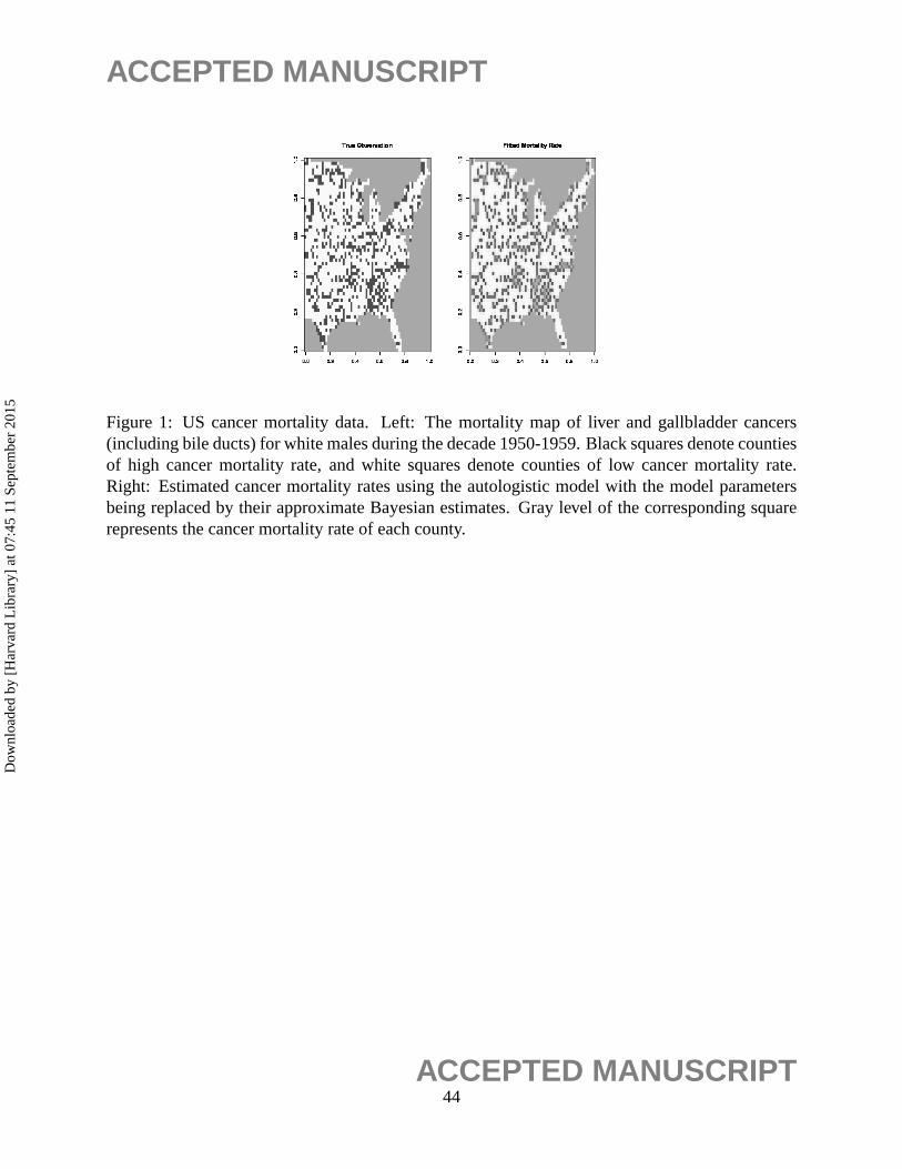
ACCEPTED MANUSCRIPT
Figure 1: US cancer mortality data. Left: The mortality map of liver and gallbladder cancers(including bile ducts) for white males during the decade 1950-1959. Black squares denote countiesof high cancer mortality rate, and white squares denote counties of low cancer mortality rate.Right: Estimated cancer mortality rates using the autologistic model with the model parametersbeing replaced by their approximate Bayesian estimates. Gray level of the corresponding squarerepresents the cancer mortality rate of each county.
44ACCEPTED MANUSCRIPT
Dow
nloa
ded
by [
Har
vard
Lib
rary
] at
07:
45 1
1 Se
ptem
ber
2015

ACCEPTED MANUSCRIPT
-0.45 -0.40 -0.35 -0.30 -0.25 -0.20 -0.15
0.05
0.10
0.15
0.20
α
β
ooooooooo
ooooooooooooooooooo
o
o
oooo
o
oooooooooooo
o
ooooooo
oo o
oo
oooooo
ooooooo
oooooo
oo
ooooooooooooooo
oo
ooooo
oo
oooooooooo
o
o
ooooooo
oooo
ooo
o oooooooooooooo
oo
ooo
o
oooo
ooo
o
o
oo
o
o
ooooo
oooo
ooo
ooo
ooooooooooo
o
o
o
ooooo
o
ooooo
o
oo
o
ooo
o
ooo
o
ooooooooo
ooo
o
ooooooo
oooooo
oo
ooo
o
oooooooooo
oo
ooo
o
oooo
o
ooooooo
oo
ooo
ooooo
oo
o
ooo
ooo
ooooo
oo
ooo
oooo
oo
o
o
o
oooooo
oo
ooooo
ooooo
o
oo
oooo
oo
oo
oooooooooooo
oo
oo
ooooooooo
oo
ooooooo
o
oo
o
ooooooo
oooooooooo
oo
o
o
oo
oo
oo
ooooo
oo
oo
ooooo
oooooooo
ooo
ooooo
o oo
oooooooooo
oooo
oooooo
ooooo
oo
o
ooo
oo
ooo
ooooooo
oooo
ooo
oooo
ooooooooooo
oooooooo
o
o
ooooooo
oooooooo
ooooo
o
o
o
ooo
ooo
o
ooooo
oo
oooooooo
oo
ooooooooo
ooo
o
oo
oo
o
o
oooooooo
o
oo
o
oooooooo
ooo
oo
ooo
o
ooooo
oooo
oo
oooooo
oooo
ooo
oo
oooooooo
o
oo
oooo
oooo
oo
oo
ooo
oo
o
oooooo
oo
oo
oo
oo
oo
oo
ooooo
o
oo
oo
oooo
ooo
ooo
ooooooooooooooooooooooo
oooooooooooooo
oooooooo
oooooooooooooooooo
o
oooooo
ooooooooo
ooooo
o
oo
ooooooo
ooo ooooo
o
ooo
ooooo
o
oo
ooo
o
o
o
ooooo
o
o
oo
ooooooo
o
o
ooooooo
ooo
oo
oo
oo
o
o
ooo
ooo
ooooooo
oooo
o
oooooo
o
oo
oooo
oooooooooooooooooo
ooooo
oo
oooo
oo
o
oo
o
o
oooooooo
ooo
o
oo
oooo
ooo ooo
ooooo
oo
ooo
oo
oo
oo
oo
oo
ooo
oooooooooo
oooo
oooo
ooo
ooo
o
oooooooooo
oo
ooooo
oo
ooooooooooooooo
ooo
oo
ooooooooooooo
oooo
ooooooooooooo
o
oooooooo
ooooo
oo
oooo
oo
o
oo
o
o
oooooo
o
oo
oooooooo
oooo
oooooo
ooooooo
oooooooooooooo
oo
ooooooo
o
oo
oo
oooooo
oo
ooooooo
ooo
ooo
o
o
o
oo
ooooooooooo
oo
oooo
oo
oooo
ooooooooo
o oooooo
o
oooooo
ooo
ooooo
ooo
ooooo
o
oooo
o
oo
oooo
ooooo
o
o
ooo
oo
o
o
oooo
ooooo
ooo
oo
oo
oooo
ooooooo
ooo
oooo
ooo
oo
oooooooo
ooo
o
oooo
o
o
oo
oooo
ooo
ooo
ooo
ooooooooo
o
o
o
o
oooooooo
ooooo
o
oooo
oooo
oooo
oo o
oooooooooooo
ooo
o
o
o
o
oo
o
ooo
ooooo
oo
o
ooooo
o
oooooooo
ooo
ooo
oo
o
o
oo
o
o
oooooooooo
o
oooo
oo
ooooo
ooo
ooooo
o
oo
ooo
oooooooooo
oooooo
oooooooooooo
oo
o
ooooooooo
ooo
ooo
ooooooooooooooooo
ooooo
oo
ooooo
oo
o
oooooo
oooooo
o
oooo
o
ooo
oo
oooo
oooo
oooooooo
oooooooooooo
oooo
oooo
oo
o
oo
o
oo
oo
ooooooooooo
o
o
oooo
oooooo
o
ooo
oooo
ooo
oooooo
o
oo
oooo
ooo
o
oo
oo
o
ooo
oooo
o
o
o
o
ooo
oo
ooooo
oooooo
oo
ooo
o
oo
oo
oooo
oo
ooooo
ooooooooooo
ooooo
o
oo
oo
oo
ooooo
ooooooooooooo
o
oo
o
o
oo
oooo
oo
oo
oooo
o
ooo
ooo
oo
o
o
ooo
ooooooooooo
oo
oooo
oooooooooo
oooooooo
oooo
o
o
o
o
o
ooooo
ooooooooo
oo
oooooo
o
o
oooooooooo
ooo
ooooo
o
oo
o
ooo
o
o
oo
o
oo
oo
ooo
oo
oooo
ooooooo
oooo
oooooooo
o
ooooo
oo
ooooooooooo
o
ooooo
oooooo
o
o
o
o
ooooooo
ooo
oo
ooooooo
ooooooooo
ooo
ooo
o
oooooooo
oooooooooooooooooo
oooo
oooooooo
oo
oooooooo
oooooooo
ooo
oooooo
ooo
oooo
ooooo
oooooooooooo
o
ooooo
oo
ooooo
o
oooo
o
ooo
ooooooo
o
o
ooooooo
o
o
ooooo
oooo
o
ooo
oo
o
oo
o
oooo
oooo
o
ooo
oo
ooooooo
o
oooooo
oooo
oooooooooooooooo
ooooooooooooooooo
oooo
ooooo
ooo
oooo
oo
ooooooooo
oooooo
o
ooo
ooooooooo
oo
o
ooooo
ooooo
ooo
oooo
ooo
oooooooooooooooo
ooooo
o
ooo
oooo
oooooooooo
ooooooo
ooooooo
o
o
ooooooooooooooooo
ooooooo
o
oooooo
ooo
o
ooo
o
o
ooooo
oooo
o
ooooooooo
o
oo
oo
ooooo
ooooooo
o
ooo
ooooooo
ooooo
o
oooooo
o
o
oooooooo
oooo
o
oo
o oo
oo
oooooo
oooooo
oooooo
oooo
o
o
o
oooo
ooo
o
o
o
oooooo
oooooooooo
oooo
oo
o
o
oooo
oo
o
ooo
o
oo
oooo
o
ooo
oooo
o
oo
oooooo
o
oooo
oo
o
o
o
o
o
oooo
o
oooo
oooooooooo
oooooooooo
oooo
o
oooooooooo
o
ooooooooo
ooo
oo
ooooooo
ooo
oo
ooooooo
o
ooo
oo
ooo
ooooo
ooooooooo
ooo
o
oooo
oo
o
oooo
o
ooooooooooooo
ooooo
oo
ooooo
o
oooooooooooooo
oo
ooo
o
o
ooo
o
oo
o
o
ooooo
oooooooo
oo
o
oooo
oooooooooo
oooo
ooo
ooooooo
ooooooooo
oooooooooooooooooo
o
ooo
ooooooo
ooooooo
o
oooooo
oo
ooo
ooooooooooo
oooooo
oooo
o
o
ooo
o
oo
ooo
o ooooooooooo
oooo
oooooo
o
oooooooo
o
oooo
ooo
o
ooo
oooo
o
o
oooooo
o
o
oooooooooooooo
ooooooooo
ooo
oo
o
oo
ooo
oooooooooo
ooo
oo
oooooo
oo
oooooooo
ooooo
ooooo
o
o
oo
o
o
ooo
ooooo
ooo
o
o
oooooooooooo
oo
ooo
oooo
oooooooo
oo
ooo
oo
ooooooo
oo
oooooo
ooo
ooo
o
oo
o
ooo
oo
ooooo
oooooooooooooooooo
ooo
ooo
oooo
oooooo
oo
oo
o
oo
ooooooooooo
oo oooo
ooooooooooooooo
oo
ooooooo
o
ooo
ooo
oooooo
ooo
oo
oooo
o
ooooo
o
oooo
oo
oooo
oo
ooo
oooooooooooo
ooo
ooooo
oo
o
o
ooooooooooooo
o
oooooooo
o
oo
ooooooooo
ooo
ooo
oooooooooooo
oo
ooooooo
ooo
oo
oooo
oooooooooooooo
o
oooo
o
oooooooooooo
o
ooo
o
o
oo
oo
oooo
o
oo
oo
oooooo
oo
ooooooo
o
o
o
o
o
o
o
ooooo
ooooooo
ooo
o
ooooo
ooooo
oooo
oo
o
oooo
oo
oooo
ooooooo
oooooo
ooooo
ooooo
ooo
ooo
oooo
oo
ooooooooooooo
oooo
oo
o
oo
ooo
ooooooooooooooooo
oooooooooo
ooooo
oooooooooo
oo
oooooo
ooooooooooooooo
oo
ooo
oo
ooooooooo
oooooo
oooooo
oo
ooooo
oooo
oooooooooooooooo
o
ooooooooo
ooo
ooooooooooooooooooooo
oooo
oooooo
ooooooooo
ooooo
oo
ooo
o
oooo
oooo
oo
o
o
o
oo
o
o
ooooooo
oo
o
oo
o
oooo
oooo
ooooooooo
ooooooooo
o
oooooooo
ooooooooooo
oo
ooooo
o
ooo
oooooooooo
ooooo
oooooo
oooo
o
ooooooo
oo
o
oooo
o
oo
o
oo
oo
oooo
oooo
ooo
ooo
oooooooooo
oo
ooooooo
ooooooo
oooo
o
ooo
oooooooo
ooooo
ooooooo
ooo
o
ooooooooooooooo
oooooooooooooo
o
o
oooooo
o
oo
oo
o
ooo
oooo
oo
o
ooooooooo
o
oooooooooo
o
ooo
ooooo
ooooooo
oo
ooo
ooo
o
o
oo
oooo
o
oo
o
oooo
ooooo
o
ooo
oo
oo
oo
ooooooo
oooooo
o
oooo
oo
o
ooo
oooo
oo
o
ooooooooo
ooooo
oo
o
oo
o
ooo
oo
oooo
o
oooooo
ooooooooooooo
ooooo
o
o
ooo
o
oooooooooooo
o
oooo
o
ooo
oo
oooooooo
oo
oo
o
oo
ooo
ooo
o oooo
oooo
ooo
o
ooooooo
oo
ooooooooo
oo
o
oo
oo
oo
o
o
ooooooooooo
o
oooooooooo
oooooo
o
oo
oooooo
oooo
oooooo
o
ooo
o
ooooooo
oo
oooo
o
oo
oooo
o
oo
oooooo
oo
ooooooooooooo
oo
ooooooooooo
oooooo
ooo
oo
oooo
oooooooo
oooo
oo
ooo
o
o
oooooooo
ooooo
o
oooooooo
oooo
oo
o
oo
oo
oooooooooo
oo
o
o
ooooooooo
oooo
ooo
oooooo
o
ooooooo
ooo
oo
ooo
ooo
ooooo
ooooooooo
oo
o o
oooooooooooo
ooo
ooooo
oo
ooo
ooooo
oo
oo
o
oooooooooo
ooooo
o
oo
oooooo
oooooooo
oo
o
oo
oooooooooooooo
ooo
oo
ooooooo
oooooooooooo
o
oo
ooo
oooooooooo
ooo
ooo
ooooo
ooooo
oo
oooooo
oooooooooo
o
oo
ooo
ooooo
ooooooo
ooooooooooo
ooo
oooooooo
ooo
oo
o
ooooooo
oo
ooooo
o
o
oo
ooo
o
ooooooo
o
o
o
ooooo
ooooo
oooo
oooo
o
o oo
o oo
oooo
ooooo
ooo
o
ooo
oooooo
ooo
o oo
o
oo
o
o
oo
oooooooo
o
o
oooo
o
ooooo
oo
oo
oooooooo
oo
o
o
ooooo
o
ooo
oooooo
oooo
ooo
ooooo
o
o
oooooooooooo
oooooooooooo
ooo
oo
ooooooooooo
o
oo
oooo
oooooooo
o
oo
ooo
oooooooooooo
ooooo
oooooooooo
o
ooooo
ooooo
oooo
o
oo
o
ooooooooooooooo
o
oooooo
oo oo
ooooooo
oooo
ooo
oooo
oooooooooooooooo
oo
ooooooooo
oo
oo
oo
oooooo
oooooooo+
+
+
+
+
+
+
+
+
+
+
+
++
+
+
+
+
+
+
+
+
+
+
+
+
+
+
+
+
++
+
+
+
+
+
+
+
+
+
++
+
+
+
+
+
+
+
+
+
++
+
+
+
+
++
++
+
+
+
+
+
++
+
+
+
+
+
+
+
+
+
+
+
+
+
+
+
+
+
+
+
+
+
+
+
+
+
+
+
++
+
+
(a)
+
+
+
+
+
+
+
+
+
+
+
+
++
+
+
+
+
+
+
+
+
+
+
+
+
+
+
+
+
++
+
+
+
+
+
+
+
+
+
++
+
+
+
+
+
+
+
+
+
++
+
+
+
+
++
++
+
+
+
+
+
++
+
+
+
+
+
+
+
+
+
+
+
+
+
+
+
+
+
+
+
+
+
+
+
+
+
+
+
++
+
+
-0.45 -0.40 -0.35 -0.30 -0.25 -0.20 -0.15
0.05
0.10
0.15
0.20
α
β
o
(b)
auxiliary parameter points
020
0040
0060
0080
0010
000
(c)
Figure 2: Auxiliary parameter set construction for the U.S. Cancer Mortality example: (a) thescatter plot of the fractional DMH samples (“o”) and the selected auxiliary parameters (“+”);(b) the neighborhood (solid dots) of a selected auxiliary parameter point (big circle); and (c) thehistogram of the 100 auxiliary parameters, where each bar corresponds to an auxiliary parameter.
0 5000 10000 15000 20000
1.0
1.5
2.0
2.5
3.0
3.5
last iteration in chain
shrin
k fa
ctor
median97.5%
0 5000 10000 15000 20000
1.0
1.5
2.0
2.5
3.0
last iteration in chain
shrin
k fa
ctor
median97.5%
Figure 3: Convergence diagnostic of the adaptive exchange algorithm for the U.S. Cancer Mortalityexample: (a) Gelman-Rubin’s shrink factor for the samples ofα generated in 10 runs; (b) Gelman-Rubin’s shrink factor for the samples ofβ generated in 10 runs.
45ACCEPTED MANUSCRIPT
Dow
nloa
ded
by [
Har
vard
Lib
rary
] at
07:
45 1
1 Se
ptem
ber
2015
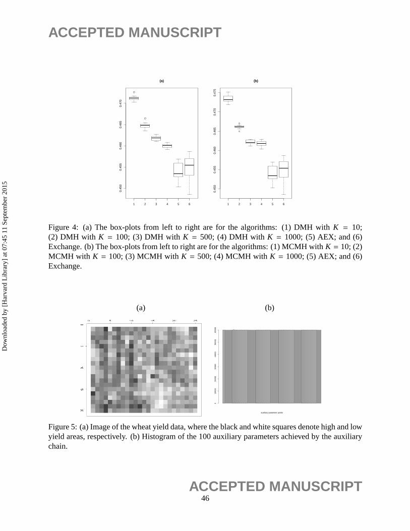
ACCEPTED MANUSCRIPT
1 2 3 4 5 6
0.45
00.
455
0.46
00.
465
0.47
0
(a)
1 2 3 4 5 6
0.45
00.
455
0.46
00.
465
0.47
00.
475
(b)
Figure 4: (a) The box-plots from left to right are for the algorithms: (1) DMH withK = 10;(2) DMH with K = 100; (3) DMH with K = 500; (4) DMH with K = 1000; (5) AEX; and (6)Exchange. (b) The box-plots from left to right are for the algorithms: (1) MCMH withK = 10; (2)MCMH with K = 100; (3) MCMH withK = 500; (4) MCMH withK = 1000; (5) AEX; and (6)Exchange.
(a) (b)
auxiliary parameter points
01
00
00
20
00
03
00
00
40
00
05
00
00
60
00
0
Figure 5: (a) Image of the wheat yield data, where the black and white squares denote high and lowyield areas, respectively. (b) Histogram of the 100 auxiliary parameters achieved by the auxiliarychain.
46ACCEPTED MANUSCRIPT
Dow
nloa
ded
by [
Har
vard
Lib
rary
] at
07:
45 1
1 Se
ptem
ber
2015
Top Related