


Languages
Pages
Legal


1 Computing and Storage Requirements
Computing and Storage Requirements for FES
J. Candy
General Atomics, San Diego, CA
Presented at
DOE Technical Program Review
Hilton Washington DC/Rockville
Rockville, MD
19-20 March 2013

2 Computing and Storage Requirements
Drift waves and tokamak plasma turbulence
Role in the context of fusion research
• Plasma performance:
In tokamak plasmas, performance is limited by turbulent radial transport of
both energy and particles.
• Gradient-driven:
This turbulent transport is caused by drift-wave instabilities, driven by free
energy in plasma temperature and density gradients.
• Unavoidable:
These instabilities will persist in a reactor.
• Various types (asymptotic theory):
ITG, TIM, TEM, ETG . . . + Electromagnetic variants (AITG, etc).

3 Computing and Storage Requirements
Fokker-Planck Theory of Plasma Transport
Basic equation still unsolved in tokamak geometry
The Fokker-Planck (FP) equation provides the fundamental theory for plasma
evolution:[
∂
∂t+ v · ∇+
eama
(
E+v
c×B
)
·∂
∂v
]
fa
=∑
b
Cab(fa, fb) + Sa
where E and B satisfy the Maxwell equations.

4 Computing and Storage Requirements
Fokker-Planck Theory of Plasma Transport
Comprehensive ordering in series of papers by Sugama and coworkers
Systematic ordering for plasma equilibrium, fluctuations, and transport:
[
∂
∂t+ v · ∇+
eama
(
(E+ E) +v
c× (B+ B)
)
·∂
∂v
]
(fa + fa)
= Ca(fa + fa) + Sa
fa −→ ensemble-averaged distribution
fa −→ fluctuating distribution
Sa −→ sources (beams, RF, etc)
Ca =∑
b
Cab(fa + fa, fb + fb) −→ nonlinear collision operator

5 Computing and Storage Requirements
Fokker-Planck theory
Comprehensive, consistent framework for equilibrium profile evolution
The general approach is to separate the FP equation into ensemble-averaged, A,
and fluctuating, F , components:
A =d
dt
∣
∣
∣
∣
ens
fa − 〈Ca〉ens −Da − Sa ,
F =d
dt
∣
∣
∣
∣
ens
fa +eama
(
E+v
c× B
)
·∂
∂v(fa + fa)− Ca + 〈Ca〉ens +Da ,
whered
dt
∣
∣
∣
∣
ens
.=
∂
∂t+ v · ∇+
eama
(
E+v
c×B
)
·∂
∂v,
Da.= −
eama
⟨
(
E+v
c× B
)
·∂fa∂v
⟩
ens
.
⊲ Da is the fluctuation-particle interaction operator.
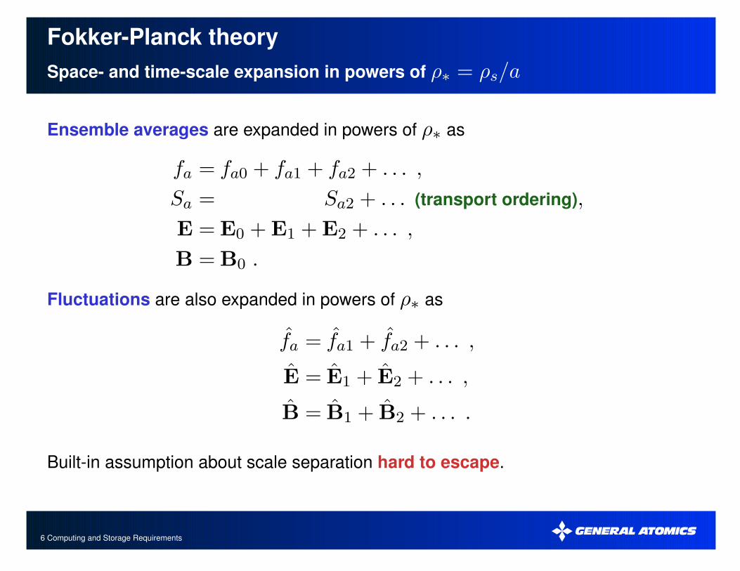
6 Computing and Storage Requirements
Fokker-Planck theory
Space- and time-scale expansion in powers of ρ∗ = ρs/a
Ensemble averages are expanded in powers of ρ∗ as
fa = fa0 + fa1 + fa2 + . . . ,
Sa = Sa2 + . . . (transport ordering),
E = E0 +E1 +E2 + . . . ,
B =B0 .
Fluctuations are also expanded in powers of ρ∗ as
fa = fa1 + fa2 + . . . ,
E = E1 + E2 + . . . ,
B = B1 + B2 + . . . .
Built-in assumption about scale separation hard to escape.

7 Computing and Storage Requirements
Fokker-Planck theory
Lowest-order conditions for flow and gyroangle independence
Lowest-order Constraints
The lowest-order ensemble-averaged equation gives the constraints
A−1 = 0 : E0 +1
cV0 ×B = 0 and
∂fa0∂ξ
= 0
where ξ is the gyroangle.
Large mean flow
The only equilibrium flow that persists on the fluctuation timescale is
V0 = Rω0(ψ)eϕ where ω0.= −c
∂Φ0
∂ψ.
[F.L. Hinton and S.K. Wong, Phys. Fluids 28 (1985) 3082].

8 Computing and Storage Requirements
Fokker-Planck theory
Equilibrium equation is a formidable nonlinear PDE
Equilibrium equation
The gyrophase average of the zeroth order ensemble-averaged equation gives the
collisional equilibrium equation:
∫ 2π
0
dξ
2πA0 = 0 :
(
V0 + v′‖b)
· ∇fa0 = Ca(fa0)
where v′ = v −V0 is the velocity in the rotating frame.
Equilibrium distribution function
The exact solution for fa0 is a Maxwellian in the rotating frame, such that the
centrifugal force causes the density to vary on the flux surface:
fa0 = na(ψ, θ)
(
ma
2πTa
)3/2
e−ma(v′)2/2Ta .

9 Computing and Storage Requirements
Fokker-Planck theory
Equations for neoclassical transport and turbulence at O(ρ∗)
Drift-kinetic equation
Gyroaverage of first-order A1 gives expressions for gyroangle-dependent (fa1) and
gyroangle-independent (fa1) distributions:
∫ 2π
0
dξ
2πA1 = 0 : fa1 = fa1 + fa1 , fa1 =
1
Ωa
∫ ξ
dξ Lfa0
⊲ Ensemble-averaged fa1 is determined by the drift kinetic equation (NEO).
Gyrokinetic equation
Gyroaverage of first-order F1 gives an expression for first-order fluctuating
distribution (fa1) in terms of the distribution of the gyrocenters, ha(R):
∫ 2π
0
dξ
2πF1 = 0 : fa1(x) = −
eaφ(x)
Ta+ ha(x− ρ)
⊲ Fluctuating fa1 is determined by the gyrokinetic equation (GYRO).

10 Computing and Storage Requirements
Drift-Kinetic Equation for Neoclassical Transport
NEO gives complete solution with full kinetic e-i-impurity coupling
v′‖b · ∇ga − CLa (ga) =
fa0
Ta
[
−1
Na
∂NaTa
∂ψWa1 −
∂Ta
∂ψWa2 + c
∂2Φ0
∂ψ2WaV +
〈BEA‖〉
〈B2〉1/2WaE
]
ga.= fa1 − fa0
ea
Ta
∫ ℓ dl
B
(
BE‖ −B2
〈B2〉〈BE‖〉
)
,
Wa1.=mac
eav′‖b · ∇
(
ω0R+I
Bv′‖
)
,
Wa2.=Wa1
(
ε
Ta−
5
2
)
,
WaV.=mac
2eav′‖b · ∇
[
ma
(
ω0R+I
Bv′‖
)
2
+ µR2B2
p
B
]
,
WaE.=eav′‖B
〈B〉1/2.

11 Computing and Storage Requirements
Gyro-Kinetic Equation for Turbulent Transport
GYRO gives complete solution with full (φ,A‖, B‖) electromagnetic physics.
∂ha(R)
∂t+(
V0 + v′‖b+ vda −c
B∇Ψa × b
)
· ∇ha(R)− CGLa
(
fa1)
=fa0
[
−∂ln(NaTa)
∂ψWa1 −
∂lnTa
∂ψWa2 +
c
Ta
∂2Φ0
∂ψ2WaV +
1
TaWaT
]
Wa1(R).= −
c
B∇Ψa × b · ∇ψ ,
Wa2(R).= Wa1
(
ε
Ta−
5
2
)
,
WaV (R).= −
maRc
B
⟨
(V0 + v′) · eϕ∇
(
φ−1
c(V0 + v
′) · A
)
× b · ∇ψ
⟩
ξ
,
WaT (R).= ea
⟨(
∂
∂t+V0 · ∇
)(
φ−1
c(V0 + v
′) · A
)⟩
ξ
.
Ψa(R).=
⟨
φ(R+ ρ)−1
c(V0 + v
′) · A(R+ ρ)
⟩
ξ
→ J0
(
k⊥v′⊥
Ωa
)
(
φ(k⊥)−V0
c· A(k⊥)−
v′‖
cA‖(k⊥)
)
+ J1
(
k⊥v′⊥
Ωa
)
v′⊥c
B‖(k⊥)
k⊥.

12 Computing and Storage Requirements
Gyro-Kinetic Equation for Turbulent Transport
GYRO gives complete solution with full (φ,A‖, B‖) electromagnetic physics.
Must also solve the electromagnetic field equations on the fluctuation scale:
1
λ2D
(
φ(x)−V0
c· A
)
= 4π∑
a
ea
∫
d3v ha(x− ρ) ,
−∇2⊥A‖(x) =
4π
c
∑
a
ea
∫
d3v ha(x− ρ)v′‖ ,
∇B‖(x)× b =4π
c
∑
a
ea
∫
d3v ha(x− ρ)v′⊥ .
⊲ Can one compute equilibrium-scale potential Φ0 from the Poisson equation?
⊲ Practically, no; need higher-order theory and extreme numerical precision.
⊲ All codes must take care to avoid nonphysical potential at long wavelength
⊲ TGYRO gets ω0(ψ) = −c∂ψΦ0 from the momentum transport equation.

13 Computing and Storage Requirements
Transport Equations
Flux-surface-averaged moments of Fokker-Planck equation
⟨∫
d3vA
⟩
θ
density
⟨∫
d3v εA
⟩
θ
energy
∑
a
⟨∫
d3v mav′ϕA
⟩
θ
toroidal momentum
Only terms of order ρ2∗ survive these averages
ρ−1∗ = 103 ρ0∗ = 1 ρ1∗ = 10−3 ρ2∗ = 10−6

14 Computing and Storage Requirements
Transport Equations
Flux-surface-averaged moments of Fokker-Planck equation to O(ρ2∗)
na(r) :∂〈na〉
∂t+
1
V ′
∂
∂r(V ′Γa) = Sn,a
Ta(r) :3
2
∂〈naTa〉
∂t+
1
V ′
∂
∂r(V ′Qa) + Πa
∂ω0
∂ψ= SW,a
ω0(r) :∂
∂t(ω0〈R
2〉∑
a
mana) +1
V ′
∂
∂r(V ′
∑
a
Πa) =∑
a
Sω,a
Sn,a = Sbeamn,a + Swall
n,a and Γa = ΓGVa + Γneo
a + Γtura
SW,a = SauxW,a + Srad
W,a + SαW,a+SturW,a+S
colW,a and Qa = QGV
a +Qneoa +Qtur
a
Πa = ΠGVa +Πneo
a +Πtura
RED: TGYRO GREEN: NEO BLUE: GYRO (TGLF)

15 Computing and Storage Requirements
Acknowledgments
Thanks for input, assistance and labour from
Yang Chen, Univ. Colorado
Stephane Ethier, PPPL
Chris Holland, UCSD
Scott Parker, Univ. Colorado
Weixing Wang, PPPL

16 Computing and Storage Requirements
Project Description
Overview and Context
The overall objective of this research is to better understand the fundamental physics
of transport (collisonal and turbulent) in tokamaks using a theoretical framework that
approximates the solution of the 6D Fokker-Planck-Landau equation. An approximate
separation of these equations into collisional (neoclassical) and turbulent (gyrokinetic)
components forms the basis of the current approach. Most of the computer time is
required by the turbulent component via massively parallel gyrokinetic simulations.
The goal is to translate this level of understanding into a predictive modeling capability
– which includes design, optimization, and interpretation of future experiments and
reactors.

17 Computing and Storage Requirements
Project Description
Overview and Context
In this report, we cover work based on the codes GTS (PPPL) and TGYRO (General
Atomics), but in the final tabulation we also include data for GEM (Univ. of Colorado).

18 Computing and Storage Requirements
Project Description
Scientific Objectives for 2017
What are your projects scientific goals for 2017? Do not limit your answer to the
computational aspect of the project.
GTS: Experimental validation for NSTX and DIII-D data is our main objective so that
we can predict the transport levels in upcoming NSTX-U (upgrade of the NSTX
experiment currently underway) and ITER experiments.

19 Computing and Storage Requirements
Project Description
Scientific Objectives for 2017
What are your projects scientific goals for 2017? Do not limit your answer to the
computational aspect of the project.

20 Computing and Storage Requirements
Project Description
Scientific Objectives for 2017
TGYRO: Having completed years of validation exercises, and identified regimes where gyrokinetic theory succeeds
and fails (so-called L-mode shortfall), we wish to continue development of “sufficiently accurate” models of turbulent
transport that can profitably be used in integrated whole-device modeling frameworks. These in turn will be used to
design and optimize future experiments. An important point is that agreement isnt perfect, but good enough to provide
actual guidance, especially with respect to uncertainty quantification. Specifically, we will continue with detailed
validation of gyrokinetic (and reduced gyrofluid) model predictions against experimental observations in US tokamaks
(DIII-D, C-Mod, NSTX) to better qualify where current models perform well, and identify parameter regimes where they
must be improved. Some attepts to understand aspects of the (near-marginal) core turbulence in ITER are also
expected.

21 Computing and Storage Requirements
Computational Strategies (now and in 2017)
Approach
Give a short, high-level description of your computational problem and your strategies
for solving it.
GTS: An important goal right now is the development of a robust algorithm for
electromagnetic, finite-beta physics in the GTS code. The more complex field
equations greatly increases the time spent in the solver, which is currently implanted
with the PETSc library routines, which is currently not multi-threaded. Since the rest of
GTS is multi-threaded, we are looking at other possible numerical solvers.
22 Computing and Storage Requirements
Computational Strategies (now and in 2017)
Approach
Give a short, high-level description of your computational problem and your strategies
for solving it.
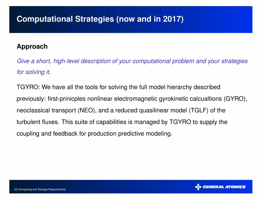
TGYRO: We have all the tools for solving the full model hierarchy described
previously: first-prinicples nonlinear electromagnetic gyrokinetic calcualtions (GYRO),
neoclassical transport (NEO), and a reduced quasilinear model (TGLF) of the
turbulent fluxes. This suite of capabilities is managed by TGYRO to supply the
coupling and feedback for production predictive modeling.

23 Computing and Storage Requirements
Computational Strategies (now and in 2017)
Codes and Algorithms
Please briefly describe your codes and the algorithms that characterize them.
GTS: The Gyrokinetic Tokamak Simulation code, GTS, is a global, gyrokinetic
particle-in-cell application in general toroidal geometry. There is also an associated
neoclassical component, GTC-NEO, the solves a time-dependent form of the
neoclassical kinetic equations using a δf particle method.

24 Computing and Storage Requirements
Computational Strategies (now and in 2017)
Codes and Algorithms
Please briefly describe your codes and the algorithms that characterize them.
TGYRO: This application combines GYRO (to solve the nonlinear electromagnetic
gyrokinetic equations using Eulerian spectral and finite-difference methods), NEO (to
solve for the neoclassical distribution and fluxes/flows with exact linearized Landau
collison operator using a spectral expansion scheme in velocity space), and TGLF (as
a proxy to GYRO using a fast quaslinear model that approximates the turbulent
transport coefficients). TGYRO itself is a transport manager that couples the above
modules to give steady-state profile prediction, as a function of input heating power,
for existing devices and future devices.

25 Computing and Storage Requirements
HPC Resources Used Today
Computational Hours
NERSC will enter the hours your project used at NERSC in 2012. If you have
significant allocations and usage at other sites please describe them here.
None at the moment
Data and I/O
How much storage space do you typically use today at NERSC for the following three
categories?
NOTE: a single TGYRO ensemble run for m1574 created 55GB data. When carrying
out many ensemble runs, not all data from each ensemble must be archived (some
users care only about transport coefficients). This means that, realistically, less than
1TB of storage will be required per user per year.

26 Computing and Storage Requirements
HPC Resources Used Today
Data and I/O
Scratch (temporary) space:
5 TB/user (GTS), < 500 GB/user (GYRO)
Permanent (can be shared, NERSC Global Filesystem /project):
20 TB / 4 TB (GTS), < 1 TB/user (GYRO)
HPSS permanent archival storage:
60 TB (GTS), < 1 TB (GYRO)

27 Computing and Storage Requirements
HPC Resources Used Today
Data and I/O
Please briefly describe your usage of these three types of storage and their
importance to your project.
Nothing out of the ordinary: the scratch filesystem is where we run all of our
simulations. We share codes and data with the other members of our project through
the project space. We archive important simulation data in HPSS.
Between which NERSC systems do you need to share data?
Hopper, Carver, Edison, dtn.

28 Computing and Storage Requirements
HPC Resources Used Today
Data and I/O
If you have experienced problems with data sharing, please explain.
On the contrary, the project area has greatly facilitated data sharing.
How do your codes perform I/O?
GTS: Some parallel I/O with ADIOS library calls for large data sets and
checkpoint-restart, as well as single-core FORTRAN ASCII I/O.
TGYRO: Large restart files are written via MPI-IO, simulation data written in ASCII,
option for HDF5 output, but not generally favoured by users.
If you have experienced problems or constraints due to I/O, please explain.

29 Computing and Storage Requirements
HPC Resources Used Today
Parallelism
How many (conventional) compute cores do you typically use for production runs at
NERSC today? What is the maximum number of cores that your codes could use for
production runs today?
GTS: Typically use 16,512 cores (2,752 MPI tasks with 6 OpenMP threads/task) for a
single run, which allows us to get the most out of our allocation. To code can scale to
a larger number of cores but the efficiency of the solver goes down due to the lack of
multithreading in PETSc. Weak scaling is more important in order to simulate ITER
plasmas.

30 Computing and Storage Requirements
HPC Resources Used Today
Parallelism
How many (conventional) compute cores do you typically use for production runs at
NERSC today? What is the maximum number of cores that your codes could use for
production runs today?
TGYRO: Typical TGYRO ensemble run with synthetic diagnostics uses 42,240 cores
(11 GYRO instances each using 1280 MPI tasks and 3 OpenMP threads, run for 12
hours, or 506,880 MPP-hours).

31 Computing and Storage Requirements
HPC Requirements in 2017
TGYRO note: Identifying range of scales needed for modeling burning plasma
conditions. A hugely important question: is ITG-scale physics enough, or is multiscale
required? This and other key questions to be answered in near term will impact our
future HPC requirements. Also, will we want to move towards production level sims
and ensemble UQ; how big will each ensemble element need to be? Plausible 2017
predictive workflow: improved version of TGLF or some other model as workhorse,
with GYRO “spot checks” at periodic and critical points.

32 Computing and Storage Requirements
HPC Requirements in 2017
Computational Hours Needed
How many compute hours (Hopper core-hour equivalent) will your project need for CY
2017? Include all hours your project will need to reach the scientific goals you listed in
1.2 above. If you expect to receive significant allocations from sources other than
NERSC, please list them here. What is the primary factor driving the need for more
hours?
GTS: We expect our project to need between 200M to 300M core-hours during CY
2017 for ITER simulations with finite-beta physics.
TGYRO: Probably about 100M core hours.

33 Computing and Storage Requirements
HPC Requirements in 2017
Data and I/O
For each of the three categories of data storage described in 3.2, above, list the
storage capacity and I/O rates (bandwidth in GB/sec, if known) that you will need in
2017. What are the primary factors driving any storage capacity and/or bandwidth
increases?
GTS: ITER data sets will be much larger so the I/O numbers should increase by about
an order of magnitude.
TGYRO: We do not expect data needs to increase significantly per user – perhaps by
a factor of 2 or 3. However, in the future we envision an increasing number of TGYRO
users.

34 Computing and Storage Requirements
HPC Requirements in 2017
Scientific Achievements with 32X Current Resources
Historically, NERSC computing resources have approximately doubled each year. If
your requirements for computing and/or data requirements listed in 4.1 and 4.2 are
less than 32X your 2012 usage, briefly describe what you could achieve scientifically
by 2017 with access to 2X more resources each year.

35 Computing and Storage Requirements
HPC Requirements in 2017
Scientific Achievements with 32X Current Resources
One could probably achieve as much by reducing bureaucracy and barriers to
resource usage as could be by adding more computational resources. The
ease-of-access to NERSC resources is valuable and should be maintained. Moreover,
true scientific advances require improvements on 2 fronts: (1) better coupling and
workflow for predictive simulations of the type achievable today, (2) an improved
theoretical formulation that can treat the pedestal and separatrix correctly – using
perhaps the original 6D FPL equation. This is a new area which goes beyond
traditional gyrokinetic. There is no accepted approach and no codes to solve this
problem. By 2017, we suspect there will be. To reiterate, progress in (2) is a matter of
progress in theoretical physics much apart from access to resources.

36 Computing and Storage Requirements
HPC Requirements in 2017
Parallelism
How many conventional (e.g., Hopper) compute cores will your code(s) be able to use
effectively in 2017? (If you expect to be using accelerators or GPUs in 2017, please
discuss this in 4.7 below.) Will you need more than one job running concurrently? If
yes, how many?
GTS: We have already demonstrated with another gyrokinetic PIC code, GTCP, that
we can achieve very high scalability (> 700,000 cores) by adding a radial domain
decomposition along with optimized multi-threading and data layout. The same
optimizations can be implemented in GTS in order to improve efficiency and
scalability.

37 Computing and Storage Requirements
HPC Requirements in 2017
Parallelism
How many conventional (e.g., Hopper) compute cores will your code(s) be able to use
effectively in 2017? (If you expect to be using accelerators or GPUs in 2017, please
discuss this in 4.7 below.) Will you need more than one job running concurrently? If
yes, how many?
TGYRO: We expect to be using GPUs in 2017, and effort is underway now to develop
this capability on titan at ORNL. We believe that the GYRO/TGYRO framework is now
maximally parallelized using MPI and OpenMP, with scalability beyond 100K cores if
required. By 2017 we expect to also solving more complex 6D equations, and we
cannot make projections about that for 2017.
38 Computing and Storage Requirements
HPC Requirements in 2017
Memory
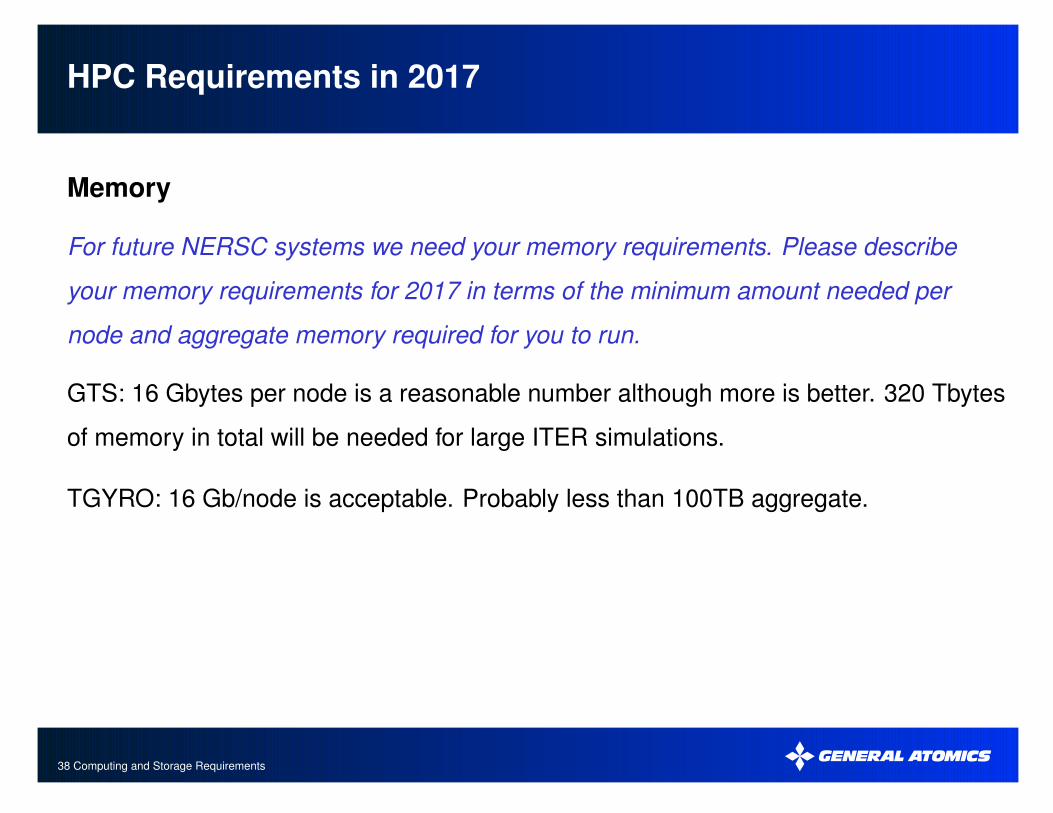
For future NERSC systems we need your memory requirements. Please describe
your memory requirements for 2017 in terms of the minimum amount needed per
node and aggregate memory required for you to run.
GTS: 16 Gbytes per node is a reasonable number although more is better. 320 Tbytes
of memory in total will be needed for large ITER simulations.
TGYRO: 16 Gb/node is acceptable. Probably less than 100TB aggregate.

39 Computing and Storage Requirements
HPC Requirements in 2017
Many-Core and/or GPU Architectures
It is expected that in 2017 and beyond systems will contain a significant number of
“lightweight” cores and/or hardware accelerators (e.g., GPUs). Are your codes ready
for this? If yes, please explain your strategy for exploiting these technologies. If not,
what are your plans for dealing with such systems and what do you need from NERSC
to help you successfully transition to them?
Our codes use OpenMP multi-threading and we are actively working on a GPU port of
key routines to take advantage of this specialized architecture for both GTS and
GYRO.

40 Computing and Storage Requirements
HPC Requirements in 2017
Software Applications and Tools
What HPC software (applications/libraries/tools/compilers/languages) will you need
from NERSC in 2017? Make sure to include analytics applications and/or I/O software.
GTS: Unless we find something better we will still use the PETSc library to implement
our solvers, as well as a random number generator (SPRNG) and spline routines
(PSPLINE). Our I/O is implemented with ADIOS.
TGYRO: netCDF, multithreaded fftw3, BLAS, LAPACK, mumps/superlu, HDF5.

41 Computing and Storage Requirements
HPC Requirements in 2017
HPC Services
What NERSC services will you require in 2017? Possibilities include consulting or
account support, data analytics and visualization, training, collaboration tools, web
interfaces, federated authentication services, gateways, etc.
All of the above.

42 Computing and Storage Requirements
Requirements Summary Worksheet
Table 1: Present and Future Requirements (GTS)
Used at NERSC in 2012 Used at NERSC in 2017
Computational Hours
(Hopper core-hour equivalent) 14.5 Million 300 Million
Scratch storage 5 TB 100TB
Scratch bandwidth
Shared global storage (project) 4 TB 100TB
Shared global bandwidth
Archival storage (HPSS) 60 TB 600TB
Archival bandwidth
Number of cores used for prod. runs 16512 160512
Memory per node 32 GB 32 GB
Aggregate memory 22 TB 220 TB

43 Computing and Storage Requirements
Requirements Summary Worksheet
Table 2: Present and Future Requirements (TGYRO)
Used at NERSC in 2012 Used at NERSC in 2017
Computational Hours
(Hopper core-hour equivalent) 14.7 Million (m1574) 150 Million
Scratch storage < 1 TB 10 TB
Scratch bandwidth
Shared global storage (project) < 1 TB 10 TB
Shared global bandwidth
Archival storage (HPSS) < 1 TB 10TB
Archival bandwidth
Number of cores used for prod. runs 20K 100K
Memory per node 16 GB 16 GB
Aggregate memory 10 TB 100 TB
44 Computing and Storage Requirements
Requirements Summary Worksheet
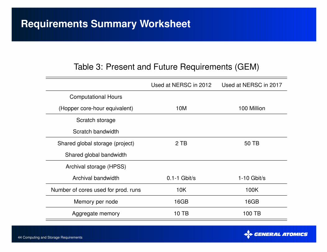
Table 3: Present and Future Requirements (GEM)
Used at NERSC in 2012 Used at NERSC in 2017
Computational Hours
(Hopper core-hour equivalent) 10M 100 Million
Scratch storage
Scratch bandwidth
Shared global storage (project) 2 TB 50 TB
Shared global bandwidth
Archival storage (HPSS)
Archival bandwidth 0.1-1 Gbit/s 1-10 Gbit/s
Number of cores used for prod. runs 10K 100K
Memory per node 16GB 16GB
Aggregate memory 10 TB 100 TB
Top Related