


Languages
Pages
Legal


Computational Imaging for VLBI Image Reconstruction
Supplemental Material
Katherine L. Bouman1 Michael D. Johnson2 Daniel Zoran1 Vincent L. Fish3
Sheperd S. Doeleman2,3 William T. Freeman1
1Computer Science and Artificial Intelligence Laboratory, Massachusetts Institute of Technology2Harvard-Smithsonian Center for Astrophysics, Harvard University
3Haystack Observatory, Massachusetts Institute of Technology
Contents
1 Additional Results and Parameters 21.1 Method Parameters and Visual Results . . . . . . . . . . . . . . . . . . . . . . . . . . . . . . . . . 21.2 EHT Telescope Parameters . . . . . . . . . . . . . . . . . . . . . . . . . . . . . . . . . . . . . . . . 261.3 Blind Test Data . . . . . . . . . . . . . . . . . . . . . . . . . . . . . . . . . . . . . . . . . . . . . . . 26
2 Energy and Optimization 282.1 Optimization Method 1 - Using Gradients . . . . . . . . . . . . . . . . . . . . . . . . . . . . . . . . 282.2 Optimization Method 2 - Taylor Expansion . . . . . . . . . . . . . . . . . . . . . . . . . . . . . . . 292.3 Derivatives . . . . . . . . . . . . . . . . . . . . . . . . . . . . . . . . . . . . . . . . . . . . . . . . . 31
3 Interstellar Scattering Kernel 333.1 Gaussian Interstellar Scattering Kernel . . . . . . . . . . . . . . . . . . . . . . . . . . . . . . . . . . 33
4 Noise 344.1 Visiblity Noise . . . . . . . . . . . . . . . . . . . . . . . . . . . . . . . . . . . . . . . . . . . . . . . 344.2 Bispectrum Noise . . . . . . . . . . . . . . . . . . . . . . . . . . . . . . . . . . . . . . . . . . . . . . 344.3 Gaussian Noise Model for the Bispectrum Including Amplitude Error . . . . . . . . . . . . . . . . . 34
1

1 Additional Results and Parameters
1.1 Method Parameters and Visual Results
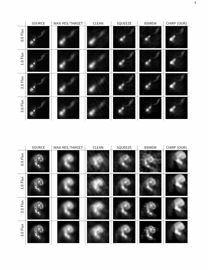
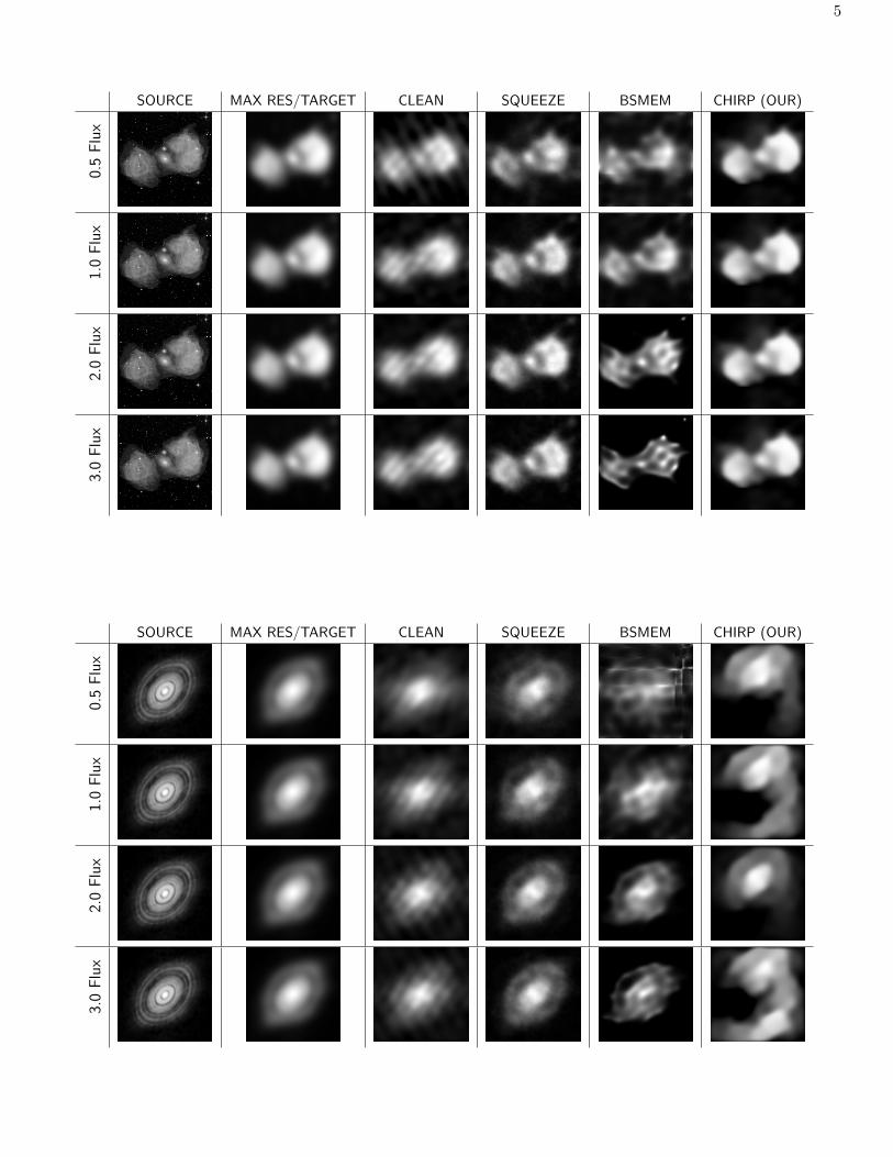
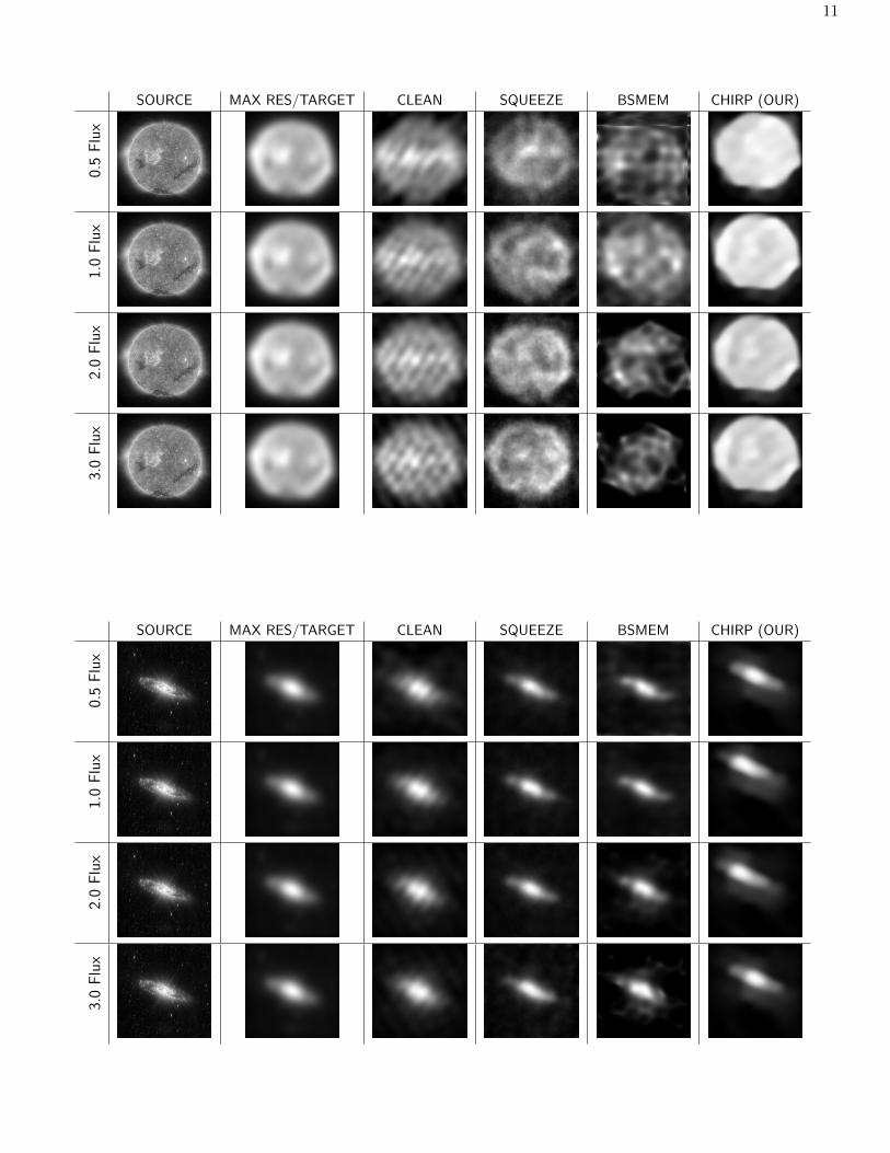
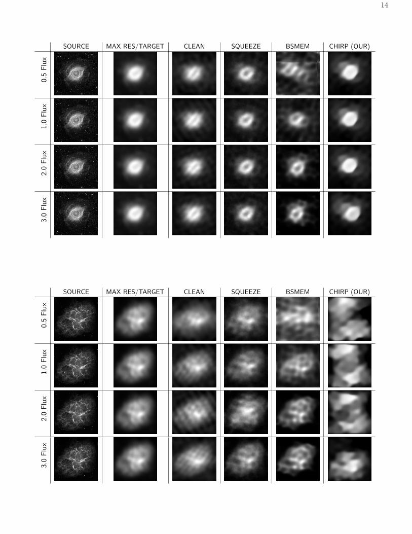
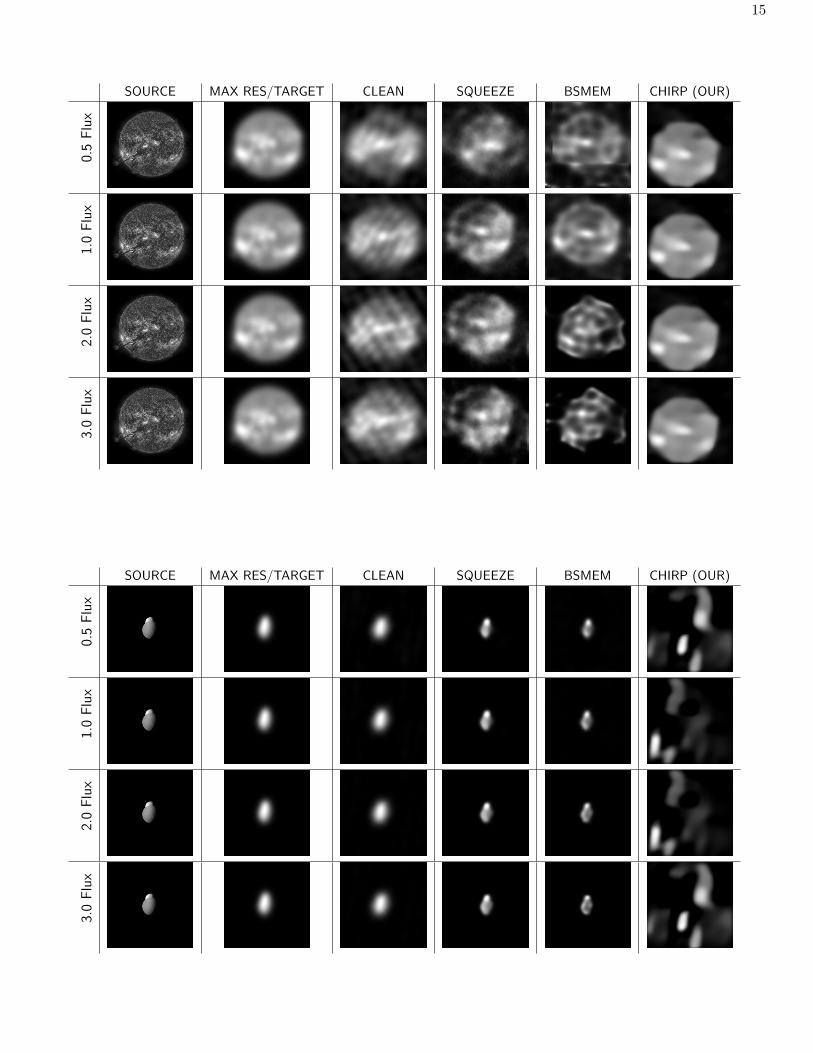
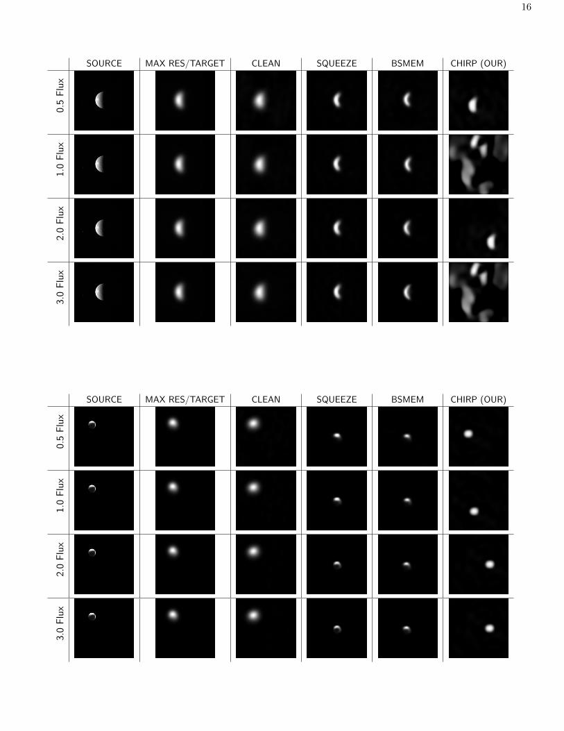
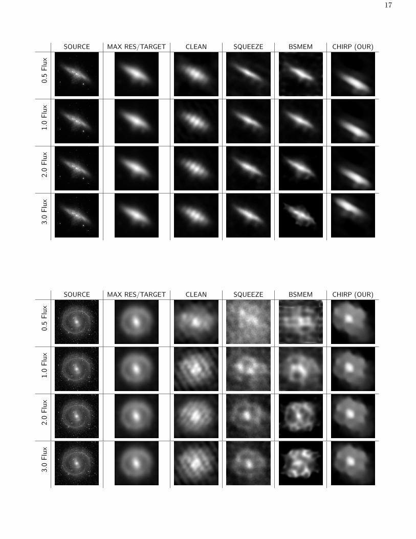
We compare results from our algorithm, CHIRP, with the three state-of-the-art algorithms described in Section 3of our paper. As with our algorithm, SQUEEZE [1] and BSMEM [2] use the bispectrum as input. To eliminatebias, images were obtained by asking either the authors of the competing algorithms or knowledgeable users forreconstruction parameters. CLEAN was run using the calibrated (eg. no phase error) visibilities inCASA [3]. In reality, these ideal calibrated visibilities would not be available, and the phase wouldneed to be recovered through highly user-dependent self-calibration methods. However, in the interestof a fair comparison, we show the results of CLEAN in a “best-case” scenario.
For image results presented, we use synthetic data corresponding to parameters of the EHT telescope array(Refer to Section 1.2) when pointed towards the black hole in M87. The specific parameters used are:
• FOV Center Right Ascension (HH:MM:SS.SS): 12:30:49.423382
• FOV Center Declination(DD:MM:SS.SS): 12:23:28.04366
• FOV Size: 0.00018382 x 0.00018382 arcseconds
• Array: EHT (Parameters in Section 1.2)
• Center Frequency: 227297 MHz
• Bandwidth: 4096 MHz
• Integration Time: 12 seconds
fov = 0.00018382numberOfPixels = 64CLEAN command: clean(vis=msFile,imagename=cleanFile, cell= str(fov/numberOfPixels*1000) +’arcsec’, threshold=’0.001Jy’, weighting=’briggs’, imsize=[numberOfPixels, numberOfPixels])SQUEEZE command: ’./src/squeeze ’ + dataPath + ’/’ + filename + ’ -s ’+str(fov/numberOfPixels*1000) + ’ -w 64 -fs ’ + str(totalFlux) + ’ -tv 3000 -e 10000 -novis’BSMEM command: ’./src/bsmem -d ’ + dataPath + ’/’ + filename + ’ -mt 0 -mf ’ + str(totalFlux)+ ’ -p ’ + str(fov/numberOfPixels*1000) + ’ -w ’ + str(numberOfPixels) + ’ -wavmin 0 -wavmax20000000 -it 20 < bsmem.batch’bsmem.batch file contents:batchdo 10centerdo 10centerdo 10centerdo 10centerdo 10centerdo 10centerdo 10centerdo 10centerdo 10centerdo 10do 20writefits output.fitsexit
We show results for each image with varying levels of noise. The standard deviation of thermal noise introducedin each measured visibility is fixed based on measurement choices and the corresponding telescopes’ intrinsicproperties. Consequently, a source emitting a lower total flux density will result in a signal with lower SNR.
2

3
SOURCE MAX RES / TARGET CLEAN SQUEEZE BSMEM CHIRP (OUR)0.5Flux
1.0Flux
2.0Flux
3.0Flux
SOURCE MAX RES/TARGET CLEAN SQUEEZE BSMEM CHIRP (OUR)
0.5Flux
1.0Flux
2.0Flux
3.0Flux
4
SOURCE MAX RES/TARGET CLEAN SQUEEZE BSMEM CHIRP (OUR)0.5Flux
1.0Flux
2.0Flux
3.0Flux
SOURCE MAX RES/TARGET CLEAN SQUEEZE BSMEM CHIRP (OUR)
0.5Flux
1.0Flux
2.0Flux
3.0Flux
5
SOURCE MAX RES/TARGET CLEAN SQUEEZE BSMEM CHIRP (OUR)0.5Flux
1.0Flux
2.0Flux
3.0Flux
SOURCE MAX RES/TARGET CLEAN SQUEEZE BSMEM CHIRP (OUR)
0.5Flux
1.0Flux
2.0Flux
3.0Flux

6
SOURCE MAX RES/TARGET CLEAN SQUEEZE BSMEM CHIRP (OUR)0.5Flux
1.0Flux
2.0Flux
3.0Flux
SOURCE MAX RES/TARGET CLEAN SQUEEZE BSMEM CHIRP (OUR)
0.5Flux
1.0Flux
2.0Flux
3.0Flux

7
SOURCE MAX RES/TARGET CLEAN SQUEEZE BSMEM CHIRP (OUR)0.5Flux
1.0Flux
2.0Flux
3.0Flux
SOURCE MAX RES/TARGET CLEAN SQUEEZE BSMEM CHIRP (OUR)
0.5Flux
1.0Flux
2.0Flux
3.0Flux

8
SOURCE MAX RES/TARGET CLEAN SQUEEZE BSMEM CHIRP (OUR)0.5Flux
1.0Flux
2.0Flux
3.0Flux
SOURCE MAX RES/TARGET CLEAN SQUEEZE BSMEM CHIRP (OUR)
0.5Flux
1.0Flux
2.0Flux
3.0Flux

9
SOURCE MAX RES/TARGET CLEAN SQUEEZE BSMEM CHIRP (OUR)0.5Flux
1.0Flux
2.0Flux
3.0Flux
SOURCE MAX RES/TARGET CLEAN SQUEEZE BSMEM CHIRP (OUR)
0.5Flux
1.0Flux
2.0Flux
3.0Flux

10
SOURCE MAX RES/TARGET CLEAN SQUEEZE BSMEM CHIRP (OUR)0.5Flux
1.0Flux
2.0Flux
3.0Flux
SOURCE MAX RES/TARGET CLEAN SQUEEZE BSMEM CHIRP (OUR)
0.5Flux
1.0Flux
2.0Flux
3.0Flux
11
SOURCE MAX RES/TARGET CLEAN SQUEEZE BSMEM CHIRP (OUR)0.5Flux
1.0Flux
2.0Flux
3.0Flux
SOURCE MAX RES/TARGET CLEAN SQUEEZE BSMEM CHIRP (OUR)
0.5Flux
1.0Flux
2.0Flux
3.0Flux

SOURCE MAX RES/TARGET CLEAN SQUEEZE BSMEM CHIRP (OUR)
0.5Flux
1.0Flux
2.0Flux
3.0Flux
SOURCE MAX RES/TARGET CLEAN SQUEEZE BSMEM CHIRP (OUR)
0.5Flux
1.0Flux
2.0Flux
3.0Flux
12

13
SOURCE MAX RES/TARGET CLEAN SQUEEZE BSMEM CHIRP (OUR)0.5Flux
1.0Flux
2.0Flux
3.0Flux
SOURCE MAX RES/TARGET CLEAN SQUEEZE BSMEM CHIRP (OUR)
0.5Flux
1.0Flux
2.0Flux
3.0Flux
14
SOURCE MAX RES/TARGET CLEAN SQUEEZE BSMEM CHIRP (OUR)0.5Flux
1.0Flux
2.0Flux
3.0Flux
SOURCE MAX RES/TARGET CLEAN SQUEEZE BSMEM CHIRP (OUR)
0.5Flux
1.0Flux
2.0Flux
3.0Flux
15
SOURCE MAX RES/TARGET CLEAN SQUEEZE BSMEM CHIRP (OUR)0.5Flux
1.0Flux
2.0Flux
3.0Flux
SOURCE MAX RES/TARGET CLEAN SQUEEZE BSMEM CHIRP (OUR)
0.5Flux
1.0Flux
2.0Flux
3.0Flux
16
SOURCE MAX RES/TARGET CLEAN SQUEEZE BSMEM CHIRP (OUR)0.5Flux
1.0Flux
2.0Flux
3.0Flux
SOURCE MAX RES/TARGET CLEAN SQUEEZE BSMEM CHIRP (OUR)
0.5Flux
1.0Flux
2.0Flux
3.0Flux
17
SOURCE MAX RES/TARGET CLEAN SQUEEZE BSMEM CHIRP (OUR)0.5Flux
1.0Flux
2.0Flux
3.0Flux
SOURCE MAX RES/TARGET CLEAN SQUEEZE BSMEM CHIRP (OUR)
0.5Flux
1.0Flux
2.0Flux
3.0Flux

18
SOURCE MAX RES/TARGET CLEAN SQUEEZE BSMEM CHIRP (OUR)0.5Flux
1.0Flux
2.0Flux
3.0Flux
SOURCE MAX RES/TARGET CLEAN SQUEEZE BSMEM CHIRP (OUR)
0.5Flux
1.0Flux
2.0Flux
3.0Flux

19
SOURCE MAX RES/TARGET CLEAN SQUEEZE BSMEM CHIRP (OUR)0.5Flux
1.0Flux
2.0Flux
3.0Flux
SOURCE MAX RES/TARGET CLEAN SQUEEZE BSMEM CHIRP (OUR)
0.5Flux
1.0Flux
2.0Flux
3.0Flux

SOURCE MAX RES/TARGET CLEAN SQUEEZE BSMEM CHIRP (OUR)
0.5Flux
1.0Flux
2.0Flux
3.0Flux
SOURCE MAX RES/TARGET CLEAN SQUEEZE BSMEM CHIRP (OUR)
0.5Flux
1.0Flux
2.0Flux
3.0Flux
20

21
SOURCE MAX RES/TARGET CLEAN SQUEEZE BSMEM CHIRP (OUR)0.5Flux
1.0Flux
2.0Flux
3.0Flux
SOURCE MAX RES/TARGET CLEAN SQUEEZE BSMEM CHIRP (OUR)
0.5Flux
1.0Flux
2.0Flux
3.0Flux

22
SOURCE MAX RES/TARGET CLEAN SQUEEZE BSMEM CHIRP (OUR)0.5Flux
1.0Flux
2.0Flux
3.0Flux
SOURCE MAX RES/TARGET CLEAN SQUEEZE BSMEM CHIRP (OUR)
0.5Flux
1.0Flux
2.0Flux
3.0Flux

23
SOURCE MAX RES/TARGET CLEAN SQUEEZE BSMEM CHIRP (OUR)0.5Flux
1.0Flux
2.0Flux
3.0Flux
SOURCE MAX RES/TARGET CLEAN SQUEEZE BSMEM CHIRP (OUR)
0.5Flux
1.0Flux
2.0Flux
3.0Flux

24
SOURCE MAX RES/TARGET CLEAN SQUEEZE BSMEM CHIRP (OUR)0.5Flux
1.0Flux
2.0Flux
3.0Flux
SOURCE MAX RES/TARGET CLEAN SQUEEZE BSMEM CHIRP (OUR)
0.5Flux
1.0Flux
2.0Flux
3.0Flux

25
SOURCE MAX RES/TARGET CLEAN SQUEEZE BSMEM CHIRP (OUR)
0.5Flux
1.0Flux
2.0Flux
3.0Flux

1.2 EHT Telescope Parameters
Here we show the parameters correspoding to the telescopes in the EHT array. The locations of the telescopesdetermine what portions of the uv plane are sampled for a given source. the SEFD provides information aboutthe noise introduced on each visibility.
NAME ALMA SMTO LMT HAWAII8 PV PbBI SPT GLT CARMA8
E. LONG -67:45:11.4 -109:52:19 -97:18:53 -155:28:40.7 -3:23:33.8 05:54:28.5 -000:00:00.0 -38:25:19.1 -118:08:30.3
LAT -23:01:09.4 32:42:06 18:59:06 19:49:27.4 37:03:58.2 44:38:02.0 -90:00:00 72:35:46.4 37:16:49.6
X-POS 2225037.1851 -1828796.2 -768713.9637 -5464523.4 5088967.9 4523998.4 0 1500692 -2397431.3
Y-POS -5441199.162 -5054406.8 -5988541.7982 -2493147.08 -301681.6 468045.24 0 -1191735 -4482018.9
Z-POS -2479303.4629 3427865.2 2063275.9472 2150611.75 3825015.8 4460309.76 -6359587.3 6066409 3843524.5
SEFD 110 11900 560 4900 2900 1600 7300 4744 3500
Table 1: Parameters corresponding to the telescopes in the EHT array: East Longitude, Latitude, X-Y-Z position (meters), andSEFD (System Equivalent Flux Density)
1.3 Blind Test Data
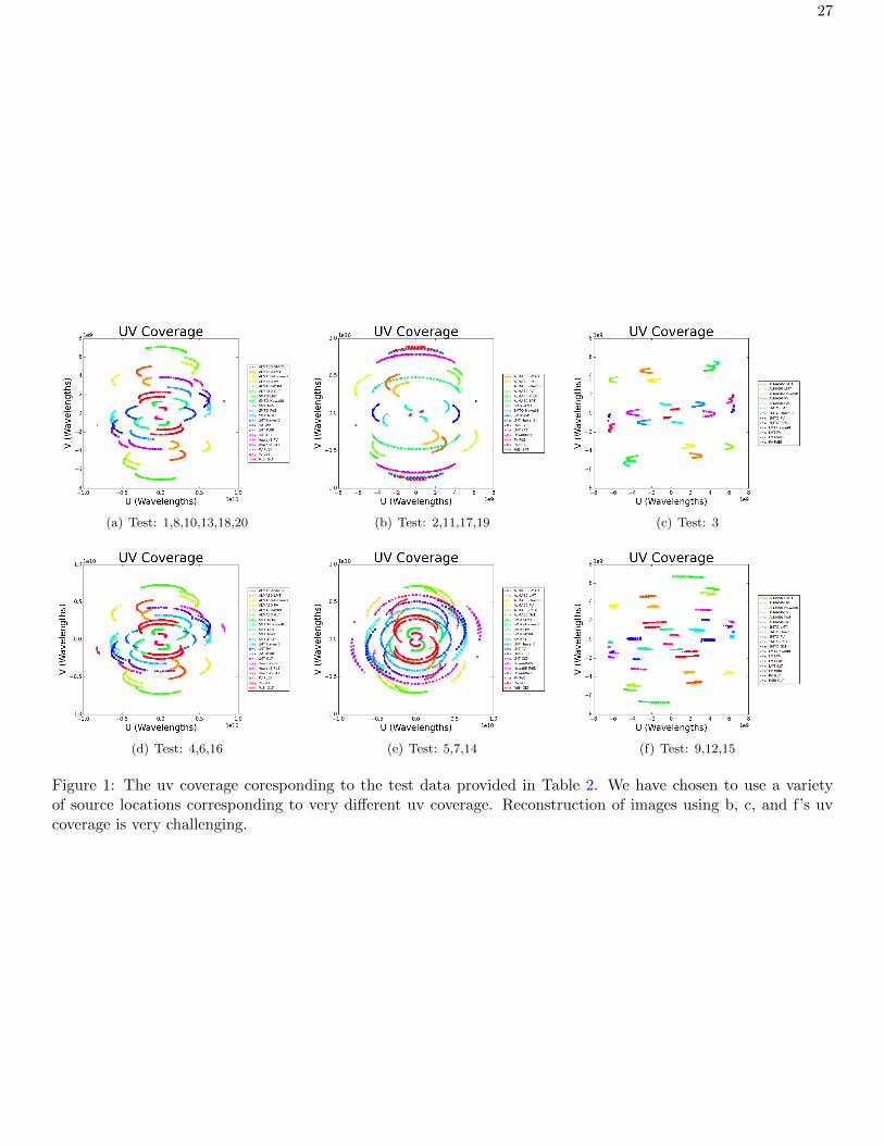
We introduce a blind test set of 20 challenging synthetic measurements. Bispectrum values along with theirsquared visibilities are generated using a variety of target sources and telescope parameters. The source/telescopeparameters that we have used for the 20 test cases can be seen in Table 2. Source locations were taken from actuallocations of black holes/blazars (M87, SgA*, 3C273, 3C279, OJ287, BL Lacertae). The EHT array’s telescopeparameters shown in Table 1 were used for simulation. The uv coverage for each of these source locations usingthe EHT array can be seen in Figure 1.
Right Ascension Declination FOV (arcsec) Center Freq (MHz) Bandwidth (MHz) Integration Time (s)
Test 1 12:30:49.423382 12:23:28.04366 0.00018382 227297 2048 10
Test 2 17:45:40.041 -29:00:28.118 0.000204595 227297 4096 10
Test 3 12:56:11.2 -05:47:21.5 0.00020264 227297 8192 10
Test 4 08:54:48.8 20:06:30 0.00018646 227297 4096 10
Test 5 22:02:43.2 42:16:40 0.00020280 227297 8192 10
Test 6 08:54:48.8 20:06:30 0.00018646 227297 2048 10
Test 7 22:02:43.2 42:16:40 0.00020280 227297 4096 10
Test 8 12:30:49.423382 12:23:28.04366 0.00018382 227297 4096 10
Test 9 12:29:6.6 02:03:08 0.00020075 227297 8192 10
Test 10 12:30:49.423382 12:23:28.04366 0.00018382 227297 8192 10
Test 11 17:45:40.041 -29:00:28.118 0.000204595 227297 4096 10
Test 12 12:29:6.6 02:03:08 0.00020075 227297 8192 10
Test 13 12:30:49.423382 12:23:28.04366 0.00018382 227297 4096 10
Test 14 22:02:43.2 42:16:40 0.00020280 227297 2048 10
Test 15 12:29:6.6 02:03:08 0.00020075 227297 8192 10
Test 16 08:54:48.8 20:06:30 0.00018646 227297 8192 10
Test 17 17:45:40.041 -29:00:28.118 0.000204595 227297 4096 10
Test 18 12:30:49.423382 12:23:28.04366 0.00018382 227297 8192 10
Test 19 17:45:40.041 -29:00:28.118 0.000204595 227297 8192 10
Test 20 12:30:49.423382 12:23:28.04366 0.00018382 227297 4096 10
Table 2: Parameters used for each of the 20 blind synthetic test data measurements. The FOV center is specified using RightAscention (HH:MM:SS.SS) and Declination(DD:MM:SS.SS).
26
27
(a) Test: 1,8,10,13,18,20 (b) Test: 2,11,17,19 (c) Test: 3
(d) Test: 4,6,16 (e) Test: 5,7,14 (f) Test: 9,12,15
Figure 1: The uv coverage coresponding to the test data provided in Table 2. We have chosen to use a varietyof source locations corresponding to very different uv coverage. Reconstruction of images using b, c, and f’s uvcoverage is very challenging.
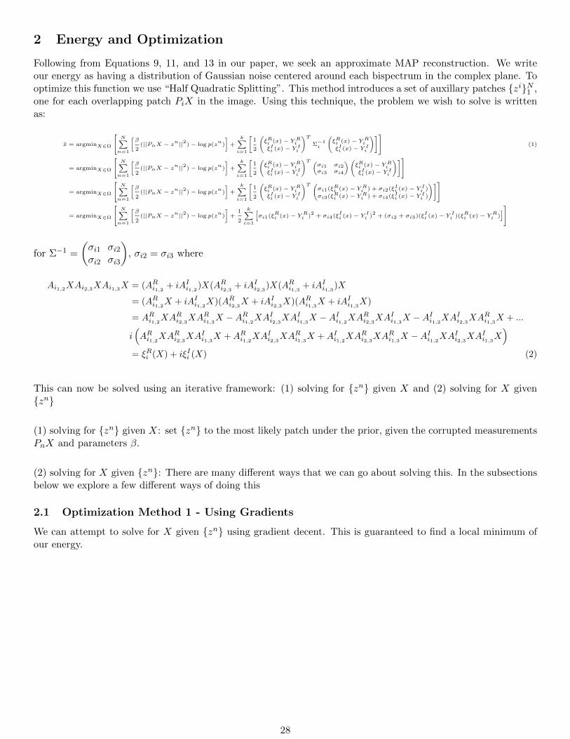
2 Energy and Optimization
Following from Equations 9, 11, and 13 in our paper, we seek an approximate MAP reconstruction. We writeour energy as having a distribution of Gaussian noise centered around each bispectrum in the complex plane. Tooptimize this function we use “Half Quadratic Splitting”. This method introduces a set of auxillary patches ziN1 ,one for each overlapping patch PiX in the image. Using this technique, the problem we wish to solve is writtenas:
x = argminX∈Ω
N∑n=1
[β
2(||PnX − zn||2)− log p(z
n)
]+
k∑i=1
[1
2
(ξRi (x)− Y R
iξIi (x)− Y I
i
)T
Σ−1i
(ξRi (x)− Y R
iξIi (x)− Y I
i
)] (1)
= argminX∈Ω
N∑n=1
[β
2(||PnX − zn||2)− log p(z
n)
]+
k∑i=1
[1
2
(ξRi (x)− Y R
iξIi (x)− Y I
i
)T (σi1 σi2σi3 σi4
)(ξRi (x)− Y R
iξIi (x)− Y I
i
)]= argminX∈Ω
N∑n=1
[β
2(||PnX − zn||2)− log p(z
n)
]+
k∑i=1
[1
2
(ξRi (x)− Y R
iξIi (x)− Y I
i
)T (σi1(ξRi (x)− Y R
i ) + σi2(ξIi (x)− Y Ii )
σi3(ξRi (x)− Y Ri ) + σi4(ξIi (x)− Y I
i )
)]= argminX∈Ω
N∑n=1
[β
2(||PnX − zn||2)− log p(z
n)
]+
1
2
k∑i=1
[σi1(ξ
Ri (x)− Y R
i )2
+ σi4(ξIi (x)− Y I
i )2
+ (σi2 + σi3)(ξIi (x)− Y I
i )(ξRi (x)− Y R
i )]
for Σ−1 =
(σi1 σi2σi2 σi3
), σi2 = σi3 where
Ai1,2XAi2,3XAi1,3X = (ARi1,2 + iAI
i1,2)X(ARi2,3 + iAI
i2,3)X(ARi1,3 + iAI
i1,3)X
= (ARi1,2X + iAI
i1,2X)(ARi2,3X + iAI
i2,3X)(ARi1,3X + iAI
i1,3X)
= ARi1,2XA
Ri2,3XA
Ri1,3X −A
Ri1,2XA
Ii2,3XA
Ii1,3X −A
Ii1,2XA
Ri2,3XA
Ii1,3X −A
Ii1,2XA
Ii2,3XA
Ri1,3X + ...
i(AR
i1,2XARi2,3XA
Ii1,3X +AR
i1,2XAIi2,3XA
Ri1,3X +AI
i1,2XARi2,3XA
Ri1,3X −A
Ii1,2XA
Ii2,3XA
Ii1,3X
)= ξRi (X) + iξIi (X) (2)
This can now be solved using an iterative framework: (1) solving for zn given X and (2) solving for X givenzn
(1) solving for zn given X: set zn to the most likely patch under the prior, given the corrupted measurementsPnX and parameters β.
(2) solving for X given zn: There are many different ways that we can go about solving this. In the subsectionsbelow we explore a few different ways of doing this
2.1 Optimization Method 1 - Using Gradients
We can attempt to solve for X given zn using gradient decent. This is guaranteed to find a local minimum ofour energy.
28

d
dXE =
d
dX
N∑n=1
[β
2(||PnX − zn||2)− log p(z
n)
]+
d
dX
1
2
k∑i=1
[σi1(ξ
Ri (x)− Y R
i )2
+ σi4(ξIi (x)− Y I
i )2
+ (σi2 + σi3)(ξIi (x)− Y I
i )(ξRi (x)− Y R
i )]
=d
dX
N∑n=1
[β
2(PnX − zn)
T(PnX − zn)− log p(z
n)
]+ ...
1
2
k∑i=1
[d
dXσi1(ξ
Ri (x)− Y R
i )2
+d
dXσi4(ξ
Ii (x)− Y I
i )2
+d
dX(σi2 + σi3)(ξ
Ii (x)− Y I
i )(ξRi (x)− Y R
i )
]
=d
dX
N∑n=1
[β
2(X
TP
Tn − (z
n)T
)(PnX − zn)− log p(zn
)
]+ ...
1
2
k∑i=1
[2σi1(ξ
Ri (x)− Y R
i )dξRi (x)
dX+ 2σi4(ξ
Ii (x)− Y I
i )dξIi (x)
dX+ (σi2 + σi3)
[(ξ
Ii (x)− Y I
i )dξRi (x)
dX+dξIi (x)
dX(ξ
Ri (x)− Y R
i )
]]
=d
dX
N∑n=1
[β
2(X
TP
Tn PnX −XT
PTn z
n − (zn
)TPnX + (z
n)Tzn
)− log p(zn
)
]+ ...
k∑i=1
[σi1(ξ
Ri (x)− Y R
i )dξRi (x)
dX+ σi4(ξ
Ii (x)− Y I
i )dξIi (x)
dX+ σi2
[(ξ
Ii (x)− Y I
i )dξRi (x)
dX+dξIi (x)
dX(ξ
Ri (x)− Y R
i )
]]
=N∑
n=1
[β
2(2P
Tn PnX − 2(z
n)TPn)
]+ ...
k∑i=1
[σi1(ξ
Ri (x)− Y R
i )dξRi (x)
dX+ σi4(ξ
Ii (x)− Y I
i )dξIi (x)
dX+ σi2
[(ξ
Ii (x)− Y I
i )dξRi (x)
dX+dξIi (x)
dX(ξ
Ri (x)− Y R
i )
]](3)
Since we know the gradient of our energy function, conditioned on knowing zn, we can solve for X using gradient
decent. Refer to subsection 2.3 for the derivativesdξIi (x)dX and
dξRi (x)dX .
2.2 Optimization Method 2 - Taylor Expansion
We can attempt to solve for X given zn by doing a Taylor expansion our energy around the current estimateof X0 and solving for X in closed-form. In order to solve this equation, we must write each of these terms as aquadratic equation of X.
Terms 1 and 2 For these terms we must approximate ξRi (X) and ξIi (X) as a function linear in X. To do thiswe linearize the interior of the quadat around a point X0 to the first order term
ξi(X0) +
(dξi(x)
dX(X0)
)(X −X0) = ξi(X0)−
(dξidX
(X0)
)X0 +
(dξidX
(X0)
)X
= βi + αiX (4)
Plugging this into its full equation we get a second order equation
(ξi(X)− Yi)2 ≈ (βi + αiX − Yi)2
= (βi + αiX − Yi)T (βi + αiX − Yi) (5)
= XTαTi αiX + 2(βi − Yi)TαiX + (βi − Yi)T (βi − Yi) (6)
Term 3 D(x) = (ξIi (x) − Y Ii )(ξRi (x) − Y R
i ) is the third term. We must Taylor expand this equation around apoint X0 to the second order term to get a function quadratic in X.
29

D(X0)+
(dD(x)
dX(X0)
)(X −X0) +
1
2(X −X0)
T(dD(x)
dX2(X0)
)(X −X0)
= D(X0)−(dD(x)
dX(X0)
)X0 +
(dD(x)
dX(X0)
)X +
1
2X
T(dD(x)
dX2(X0)
)X...
−1
2X
T(dD(x)
dX2(X0)
)X0 +
1
2X
T0
(dD(x)
dX2(X0)
)X0 −
1
2X
T0
(dD(x)
dX2(X0)
)X
=
(D(X0)−
(dD(x)
dX(X0)
)X0 +
1
2X
T0
(dD(x)
dX2(X0)
)X0
)...
+
((dD(x)
dX(X0)
)−
1
2
((dD(x)
dX2(X0)
)X0
)T
−1
2X
T0
(dD(x)
dX2(X0)
))X +
1
2X
T(dD(x)
dX2(X0)
)X
=
(D(X0)−
(dD(x)
dX(X0)
)X0 +
1
2X
T0
(dD(x)
dX2(X0)
)X0
)...
+
((dD(x)
dX(X0)
)−XT
0
(dD(x)
dX2(X0)
))X +
1
2X
T(dD(x)
dX2(X0)
)X
= D0 +D1X +XTD2X (7)
where
D0 = D(X0)−(dD(x)
dX(X0)
)X0 +
1
2X
T0
(dD(x)
dX2(X0)
)X0
D1 =
(dD(x)
dX(X0)
)−XT
0
(dD(x)
dX2(X0)
)D2 =
1
2
(dD(x)
dX2(X0)
)
Since D(x) = (ξIi (x)− Y Ii )(ξRi (x)− Y R
i ) = ξIi (x)ξRi (x) + Y Ii Y
Ri − Y R
i ξIi (x)− Y I
i ξRi (x) we know that
d
dXD =
dξIi (x)
dXξRi (x) + ξ
Ii (x)
dξRi (x)
dX− Y R
i
dξIi (x)
dX− Y I
i
dξRi (x)
dX
d
dX2D =
d
dX
(d
dXD
)=
d
dX
(dξIi (x)
dXξRi (x) + ξ
Ii (x)
dξRi (x)
dX− Y R
i
dξIi (x)
dX− Y I
i
dξRi (x)
dX
)
=dξIi (x)
dX2ξRi (x) +
dξIi (x)
dX
dξRi (x)
dX
T
+ ξIi (x)
dξRi (x)
dX2+dξRi (x)
dX
dξIi (x)
dX
T
− Y Ri
dξIi (x)
dX2− Y I
i
dξRi (x)
dX2
(8)
Solution Then, we plug this quadratic form into our optimization
x = argminX∈Ω
N∑n=1
[β
2(||PnX − zn||2)− log p(z
n)
]+
1
2
k∑i=1
[σi1(β
Ri + α
Ri X − Y
Ri )
2+ σi4(β
Ii + α
IiX − Y
Ii )
2+ (σi2 + σi3)(D0 +D1X +X
TD2X)
] (9)
Now, we can just solve for X
30

d
dXE =
d
dX
N∑n=1
[β
2(||PnX − zn||2)− log p(z
n)
]+
d
dX
k∑i=1
1
2
[σi1(β
Ri + α
Ri X − Y
Ri )
2+ σi4(β
Ii + α
IiX − Y
Ii )
2+ (σi2 + σi3)(D0 +D1X +X
TD2X)
]=
N∑n=1
[β
2(2P∗Tn PnX − 2(z
n)∗TPn)
]+
d
dX
k∑i=1
1
2
[σi1(β
Ri + α
Ri X − Y
Ri )
2]
+d
dX
k∑i=1
1
2
[σi4(β
Ii + α
IiX − Y
Ii )
2]...
+d
dX
k∑i=1
1
2
[(σi2 + σi3)(D0 +D1X +X
TD2X)
]
=N∑
n=1
[β
2(2P∗Tn PnX − 2(z
n)∗TPn)
]+
d
dX
k∑i=1
σi1
2
[(β
Ri − Y
Ri )
2+ 2(β
Ri − Y
Ri )αRX +X
TαRT
αRi X
]...
+d
dX
k∑i=1
σi4
2
[(β
Ii − Y
Ii )
2+ 2(β
Ii − Y
Ii )αIX +X
TαITαIiX]
+d
dX
k∑i=1
σi2 + σi3
2
[D0 +D1X +X
TD2X
]
=N∑
n=1
[β
2(2P∗Tn PnX − 2(z
n)∗TPn)
]+
k∑i=1
σi1
2
[2(β
Ri − Y
Ri )αR + 2α
RTαRi X
]...
+k∑
i=1
σi4
2
[2(β
Ii − Y
Ii )αI + 2α
ITαIiX]
+k∑
i=1
σi2 + σi3
2[D1 + 2D2X]
=
N∑n=1
[βP∗Tn Pn
]+
k∑i=1
σi1
[αRT
αRi
]+
k∑i=1
σi4
[αITαIi
]+
k∑i=1
(σi2 + σi3)D2
X...−
N∑n=1
[β(z
n)∗TPn
]−
k∑i=1
σi1
[(β
Ri − Y
Ri )αR
]−
k∑i=1
σi4
[(β
Ii − Y
Ii )αI
]−
k∑i=1
σi2 + σi3
2D1
(10)
Therefore,
X =
N∑n=1
[βP∗Tn Pn
]+
k∑i=1
[σi1α
RTαRi + σi4α
ITαIi + (σi2 + σi3)D2
]−1
...
N∑n=1
[β(z
n)∗TPn
]−
k∑i=1
[σi1(β
Ri − Y
Ri )αR + σi4(β
Ii − Y
Ii )αI +
σi2 + σi3
2D1
](11)
X =
N∑n=1
[βP∗Tn Pn
]+
k∑i=1
[σi1α
RTαRi + σi4α
ITαIi + (σi2 + σi3)D2
]−1
...
N∑n=1
[β(z
n)∗TPn
]−
k∑i=1
[σi1(β
Ri − Y
Ri )αR + σi4(β
Ii − Y
Ii )αI +
σi2 + σi3
2D1
](12)
2.3 Derivatives
We must find the derivative of ξRi with respect to X
d
dXξRi =
d
dX
(AR
i1,2XARi2,3XA
Ri1,3X −A
Ri1,2XA
Ii2,3XA
Ii1,3X −A
Ii1,2XA
Ri2,3XA
Ii1,3X −A
Ii1,2XA
Ii2,3XA
Ri1,3X
)=
d
dX(AR
i1,2XARi2,3XA
Ri1,3X)− d
dX(AR
i1,2XAIi2,3XA
Ii1,3X)− d
dX(AI
i1,2XARi2,3XA
Ii1,3X)− d
dX(AI
i1,2XAIi2,3XA
Ri1,3X)
= ARi1,2A
Ri2,3XA
Ri1,3X +AR
i2,3ARi1,2XA
Ri1,3X +AR
i1,3ARi2,3XA
Ri1,2X...
− (ARi1,2A
Ii2,3XA
Ii1,3X +AI
i2,3ARi1,2XA
Ii1,3X +AI
i1,3AIi2,3XA
Ri1,2X)...
− (AIi1,2A
Ri2,3XA
Ii1,3X +AR
i2,3AIi1,2XA
Ii1,3X +AI
i1,3ARi2,3XA
Ii1,2X)...
− (AIi1,2A
Ii2,3XA
Ri1,3X +AI
i2,3AIi1,2XA
Ri1,3X +AR
i1,3AIi2,3XA
Ii1,2X)
Now, we derive the second derivative of ξRr with respect to X.
31

d
dX2ξRi =
d
dX
(d
dXξRi
)=
d
dX(A
Ri1,2
ARi2,3
XARi1,3
X) +d
dX(A
Ri2,3
ARi1,2
XARi1,3
)X +d
dX(A
Ri1,3
ARi2,3
XARi1,2
X)...
− (d
dX(A
Ri1,2
AIi2,3
XAIi1,3
X) +d
dX(A
Ii2,3
ARi1,2
XAIi1,3
X) +d
dX(A
Ii1,3
AIi2,3
XARi1,2
X))...
− (d
dX(A
Ii1,2
ARi2,3
XAIi1,3
X) +d
dX(A
Ri2,3
AIi1,2
XAIi1,3
X) +d
dX(A
Ii1,3
ARi2,3
XAIi1,2
X))...
− (d
dX(A
Ii1,2
AIi2,3
XARi1,3
X) +d
dX(A
Ii2,3
AIi1,2
XARi1,3
X) +d
dX(A
Ri1,3
AIi2,3
XAIi1,2
X))
= ARTi1,2
ARi2,3
ARi1,3
X + ARTi1,2
ARi1,3
ARi2,3
X + ARTi2,3
ARi1,2
ARi1,3
X + ARTi2,3
ARi1,3
ARi1,2
X + ARTi1,3
ARi2,3
ARi1,2
X + ARTi1,3
ARi1,2
ARi2,3
X...
− (ARTi1,2
AIi2,3
AIi1,3
X + ARTi1,2
AIi1,3
AIi2,3
X + AITi2,3
ARi1,2
AIi1,3
X + AITi2,3
AIi1,3
ARi1,2
X + AITi1,3
AIi2,3
ARi1,2
X + AITi1,3
ARi1,2
AIi2,3
X)...
− (AITi1,2
ARi2,3
AIi1,3
X + AITi1,2
AIi1,3
ARi2,3
X + ARTi2,3
AIi1,2
AIi1,3
X + ARTi2,3
AIi1,3
AIi1,2
X + AITi1,3
ARi2,3
AIi1,2
X + AITi1,3
AIi1,2
ARi2,3
X)...
− (AITi1,2
AIi2,3
ARi1,3
X + AITi1,2
ARi1,3
AIi2,3
X + AITi2,3
AIi1,2
ARi1,3
X + AITi2,3
ARi1,3
AIi1,2
X + ARTi1,3
AIi2,3
AIi1,2
X + ARTi1,3
AIi1,2
AIi2,3
X)
Similarly, the derivative of ξIi with respect to X is
d
dXξIi =
d
dX
(AR
i1,2XARi2,3XA
Ii1,3X +AR
i1,2XAIi2,3XA
Ri1,3X +AI
i1,2XARi2,3XA
Ri1,3X −A
Ii1,2XA
Ii2,3XA
Ii1,3X
)= AR
i1,2ARi2,3XA
Ii1,3X +AR
i2,3ARi1,2XA
Ii1,3X +AI
i1,3ARi2,3XA
Ri1,2X...
+ARi1,2A
Ii2,3XA
Ri1,3X +AI
i2,3ARi1,2XA
Ri1,3X +AR
i1,3AIi2,3XA
Ri1,2X...
+AIi1,2A
Ri2,3XA
Ri1,3X +AR
i2,3AIi1,2XA
Ri1,3X +AR
i1,3ARi2,3XA
Ii1,2X...
− (AIi1,2A
Ii2,3XA
Ii1,3X +AI
i2,3AIi1,2XA
Ii1,3X +AI
i1,3AIi2,3XA
Ii1,2X)
Now, we derive the second derivative of ξIr with respect to X.
d
dX2ξIi =
d
dX
(d
dXξIi
)=
d
dX(A
Ri1,2
ARi2,3
XAIi1,3
X) +d
dX(A
Ri2,3
ARi1,2
XAIi1,3
X) +d
dX(A
Ii1,3
ARi2,3
XARi1,2
X)...
+d
dX(A
Ri1,2
AIi2,3
XARi1,3
X) +d
dX(A
Ii2,3
ARi1,2
XARi1,3
X) +d
dX(A
Ri1,3
AIi2,3
XARi1,2
X)...
+d
dX(A
Ii1,2
ARi2,3
XARi1,3
X) +d
dX(A
Ri2,3
AIi1,2
XARi1,3
X) +d
dX(A
Ri1,3
ARi2,3
XAIi1,2
X)...
− (d
dX(A
Ii1,2
AIi2,3
XAIi1,3
X) +d
dX(A
Ii2,3
AIi1,2
XAIi1,3
X) +d
dX(A
Ii1,3
AIi2,3
XAIi1,2
X))
= ARTi1,2
ARi2,3
AIi1,3
X + ARTi1,2
AIi1,3
ARi2,3
X + ARTi2,3
ARi1,2
AIi1,3
X + ARTi2,3
AIi1,3
ARi1,2
X + AITi1,3
ARi2,3
ARi1,2
X + AITi1,3
ARi1,2
ARi2,3
X...
+ (ARTi1,2
AIi2,3
ARi1,3
X + ARTi1,2
ARi1,3
AIi2,3
X + AITi2,3
ARi1,2
ARi1,3
X + AITi2,3
ARi1,3
ARi1,2
X + ARTi1,3
AIi2,3
ARi1,2
X + ARTi1,3
ARi1,2
AIi2,3
X)...
+ (AITi1,2
ARi2,3
ARi1,3
X + AITi1,2
ARi1,3
ARi2,3
X + ARTi2,3
AIi1,2
ARi1,3
X + ARTi2,3
ARi1,3
AIi1,2
X + ARTi1,3
ARi2,3
AIi1,2
X + ARTi1,3
AIi1,2
ARi2,3
X)...
− (AITi1,2
AIi2,3
AIi1,3
X + AITi1,2
AIi1,3
AIi2,3
X + AITi2,3
AIi1,2
AIi1,3
X + AITi2,3
AIi1,3
AIi1,2
X + AITi1,3
AIi2,3
AIi1,2
X + AITi1,3
AIi1,2
AIi2,3
X)
32

3 Interstellar Scattering Kernel
So far we have assumed that the measurements we obtain from the telescopes give us a noisy measurement of thefrequency component of the true image. However, in reality, the frequency component we receive corresponds to animage that has been corrupted by interstellar scattering. Interstellar scattering essentially convolves the true, sharpimage with a kernel. From now on we will call this kernel that interstellar scattering kernel k(l,m). Suppose weknow the Fourier transform of k(l,m) at every observed frequency K(u, v). Then, our actual measured frequencycomponents are actually given by K(uim,n , vim,n)Aim,nX = Kim,nAim,nX rather than just Aim,nX. Therefore, anoptimization that removes this interstellar scattering can be written as
X = argminX∈Ω
N∑n=1
[β
2(||PnX − zn||2)− log p(z
n)
]+
k∑i=1
[1
2
(ζRi (X)− Y R
iζIi (X)− Y I
i
)T
Σ−1i
(ζRi (X)− Y R
iζIi (X)− Y I
i
)] (13)
= argminX∈Ω
N∑n=1
[β
2(||PnX − zn||2)− log p(z
n)
]+
1
2
k∑i=1
[σi1(ζ
Ri (X)− Y R
i )2
+ σi4(ζIi (X)− Y I
i )2
+ (σi2 + σi3)(ζIi (X)− Y I
i )(ζRi (X)− Y R
i )]
where the triple product is now written with the interstellar scattering kernel as
Ki1,2Ai1,2
XKi2,3Ai2,3
XKi1,3Ai1,3
X = Ki1,2Ki2,3
Ki3,1(A
Ri1,2
+ iAIi1,2
)X(ARi2,3
+ iAIi2,3
)X(ARi1,3
+ iAIi1,3
)X
= Ki1,2Ki2,3
Ki3,1(A
Ri1,2
X + iAIi1,2
X)(ARi2,3
X + iAIi2,3
X)(ARi1,3
X + iAIi1,3
X)
= Ki1,2Ki2,3
Ki3,1
(A
Ri1,2
XARi2,3
XARi1,3
X − ARi1,2
XAIi2,3
XAIi1,3
X − AIi1,2
XARi2,3
XAIi1,3
X − AIi1,2
XAIi2,3
XARi1,3
X)
+ ...
iKi1,2Ki2,3
Ki3,1
(A
Ri1,2
XARi2,3
XAIi1,3
X + ARi1,2
XAIi2,3
XARi1,3
X + AIi1,2
XARi2,3
XARi1,3
X − AIi1,2
XAIi2,3
XAIi1,3
X)
= ζRi (X) + iζ
Ii (X) (14)
If we do not include the interstellar scatting kernel into our optimization, then ideally we could deconvolveits effects out in the end. However, this would require the result of the first stage of optimization to be a blurryimage. This image would not necessarily score well on our metric for how much it looks like the true image, andas such may be not be the best solution in the first stage of optimization. To achieve the best performance, weshould include the interstellar scattering kernel into our optimization equation.
3.1 Gaussian Interstellar Scattering Kernel
The interestellar scattering introduced in the path to black hole SgA* can be estimated by a Gaussian withcovariance (radians) [4]
Σk =
(2.00614× 10⁻²¹ 3.21018× 10⁻²²
3.21018× 10⁻²² 5.64104× 10⁻²²
)(15)
Therefore, the kerenel can be described using the following equation
k(x) =1
2π|Σ|−1/2exp
[−1
2(x− µ)TΣ−1k (x− µ)
](16)
The continuos Fourier Transform of this kernel is given by
K(f) =1
2π|Σ|−1/2exp
[−2π2(f − jΣ−1k µ)TΣk(f − jΣ−1k µ)
](17)
If we assume that our kernel is centered at 0 (shouldn’t affect results at all), then since µ = 0, jΣ−1k µ also is 0.Therefore,
K(f) =1
2π|Σ|−1/2exp
[−2π2fTΣkf
](18)
where f = (u, v). This equation can be used to scale each of the extracted bispectrum terms accordingly (as isdone in Equation 14).
33
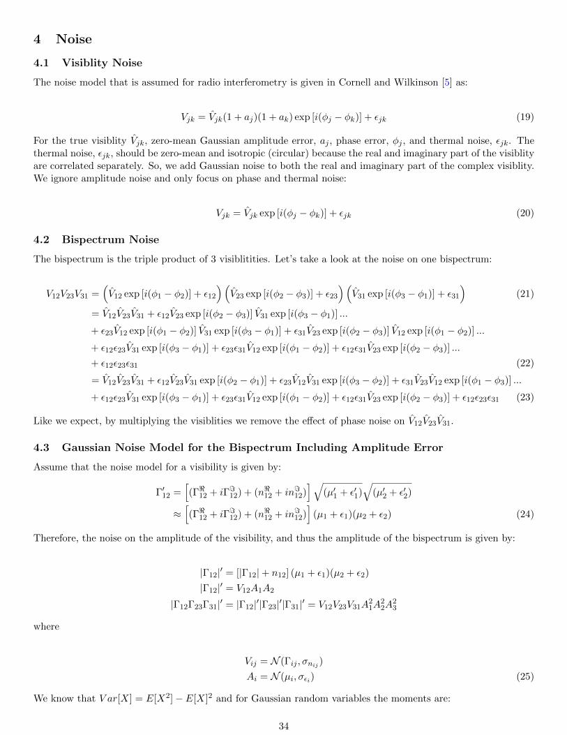
4 Noise
4.1 Visiblity Noise
The noise model that is assumed for radio interferometry is given in Cornell and Wilkinson [5] as:
Vjk = Vjk(1 + aj)(1 + ak) exp [i(φj − φk)] + εjk (19)
For the true visiblity Vjk, zero-mean Gaussian amplitude error, aj , phase error, φj , and thermal noise, εjk. Thethermal noise, εjk, should be zero-mean and isotropic (circular) because the real and imaginary part of the visiblityare correlated separately. So, we add Gaussian noise to both the real and imaginary part of the complex visiblity.We ignore amplitude noise and only focus on phase and thermal noise:
Vjk = Vjk exp [i(φj − φk)] + εjk (20)
4.2 Bispectrum Noise
The bispectrum is the triple product of 3 visiblitities. Let’s take a look at the noise on one bispectrum:
V12V23V31 =(V12 exp [i(φ1 − φ2)] + ε12
)(V23 exp [i(φ2 − φ3)] + ε23
)(V31 exp [i(φ3 − φ1)] + ε31
)(21)
= V12V23V31 + ε12V23 exp [i(φ2 − φ3)] V31 exp [i(φ3 − φ1)] ...+ ε23V12 exp [i(φ1 − φ2)] V31 exp [i(φ3 − φ1)] + ε31V23 exp [i(φ2 − φ3)] V12 exp [i(φ1 − φ2)] ...+ ε12ε23V31 exp [i(φ3 − φ1)] + ε23ε31V12 exp [i(φ1 − φ2)] + ε12ε31V23 exp [i(φ2 − φ3)] ...+ ε12ε23ε31 (22)
= V12V23V31 + ε12V23V31 exp [i(φ2 − φ1)] + ε23V12V31 exp [i(φ3 − φ2)] + ε31V23V12 exp [i(φ1 − φ3)] ...+ ε12ε23V31 exp [i(φ3 − φ1)] + ε23ε31V12 exp [i(φ1 − φ2)] + ε12ε31V23 exp [i(φ2 − φ3)] + ε12ε23ε31 (23)
Like we expect, by multiplying the visiblities we remove the effect of phase noise on V12V23V31.
4.3 Gaussian Noise Model for the Bispectrum Including Amplitude Error
Assume that the noise model for a visibility is given by:
Γ′12 =[(Γ<12 + iΓ=12) + (n<12 + in=12)
]√(µ′1 + ε′1)
√(µ′2 + ε′2)
≈[(Γ<12 + iΓ=12) + (n<12 + in=12)
](µ1 + ε1)(µ2 + ε2) (24)
Therefore, the noise on the amplitude of the visibility, and thus the amplitude of the bispectrum is given by:
|Γ12|′ = [|Γ12|+ n12] (µ1 + ε1)(µ2 + ε2)
|Γ12|′ = V12A1A2
|Γ12Γ23Γ31|′ = |Γ12|′|Γ23|′|Γ31|′ = V12V23V31A21A
22A
23
where
Vij = N (Γij , σnij )
Ai = N (µi, σεi) (25)
We know that V ar[X] = E[X2]− E[X]2 and for Gaussian random variables the moments are:
34

E[X] = µ
E[X2] = µ2 + σ2
E[X3] = µ3 + 3µσ2
E[X4] = µ4 + 6µ2σ2 + 3σ4 (26)
Therefore,
V ar[|Γ12|′|Γ23|′|Γ31|′] = E[|Γ12|′2|Γ23|′2|Γ31|′2]− E[|Γ12|′|Γ23|′|Γ31|′]2
= E[V 212V
223V
231A
41A
42A
43]− E[V12V23V31A
21A
22A
23]2
= E[V 212]E[V 2
23]E[V 231]E[A4
1]E[A42]E[A4
3]− E[V12]E[V23]E[V31]E[A21]E[A2
2]E[A23]2
= (|Γ12|2 + σ2n12)(|Γ23|2 + σ2n23
)(|Γ31|2 + σ2n31)(µ41 + 6µ21σ
2ε1 + 3σ4ε1)(µ42 + 6µ22σ
2ε2 + 3σ4ε2)(µ41 + 6µ23σ
2ε3 + 3σ4ε3)
− |Γ12|2|Γ23|2|Γ31|2(µ21 + σ2ε1)2(µ22 + σ2ε2)2(µ23 + σ2ε3)2 (27)
Gain Error Distribution Approximation Given we know the gain error parameters, µ′ and ε′, how shouldwe estimate µ and ε? Find these parameters such that
X ∼ N (µ′, σ2ε′)
Y ∼ N (µ, σ2ε )
X ≈ Y 2 (28)
If Y = 1√µ′
(µ′ + ε′/2) then X = 1µ′ (µ
′ + ε′/2)2 = µ′ + ε′ + ε′2
4µ′ . If ε′2 << µ′, then X ≈ µ′ + ε′. This implies that if
X ∼ N (µ′, σ2ε′)
Y ∼ N (√µ′,
1
4µ′σ2ε′) (29)
35

References
[1] Baron, F., Monnier, J.D., Kloppenborg, B.: A novel image reconstruction software for optical/infrared interfer-ometry. In: SPIE Astronomical Telescopes+ Instrumentation, International Society for Optics and Photonics(2010) 77342I–77342I
[2] Buscher, D.: Direct maximum-entropy image reconstruction from the bispectrum. In: Very High AngularResolution Imaging. Springer (1994) 91–93
[3] Jaeger, S.: The common astronomy software application (casa). In: Astronomical Data Analysis Software andSystems XVII. Volume 394. (2008) 623
[4] Bower, G.C., Goss, W., Falcke, H., Backer, D.C., Lithwick, Y.: The intrinsic size of sagittarius a* from 0.35to 6 cm. The Astrophysical Journal Letters 648(2) (2006) L127
[5] Cornwell, T., Wilkinson, P.: A new method for making maps with unstable radio interferometers. MonthlyNotices of the Royal Astronomical Society 196(4) (1981) 1067–1086
36
Top Related