


Languages
Pages
Legal

Comprehensive Tutorial for theSpatio-Temporal R-package
Silas BergenUniversity of Washington
Johan LindstromUniversity of Washington
Lund University
10th October 2012

Contents
Contents
1 Introduction 1
1.1 Key Assumptions . . . . . . . . . . . . . . . . . . . . . . . . . 2
1.2 Common Problems — Troubleshooting . . . . . . . . . . . . . 2
2 Data 3
2.1 NOx Observations . . . . . . . . . . . . . . . . . . . . . . . . . 3
2.1.1 Air Quality System (AQS) data . . . . . . . . . . . . . 3
2.1.2 MESA Air data . . . . . . . . . . . . . . . . . . . . . . 3
2.2 Geographic Information System (GIS) . . . . . . . . . . . . . 4
2.3 Caline Dispersion Model for Air Pollution . . . . . . . . . . . 4
3 Model and Theory 5
3.1 Model parameters . . . . . . . . . . . . . . . . . . . . . . . . . 6
4 Preliminaries 7
4.1 The STdata object . . . . . . . . . . . . . . . . . . . . . . . . 8
4.1.1 The mesa.data$covars Data Frame . . . . . . . . . . 8
4.1.2 The mesa.data$trend Data Frame . . . . . . . . . . . 11
4.1.3 The mesa.data$obs Data Frame . . . . . . . . . . . . 11
4.1.4 The mesa.data$SpatioTemporal Array . . . . . . . . 12
4.2 Summaries of mesa.data . . . . . . . . . . . . . . . . . . . . . 14
4.3 Creating an STdata object from raw data . . . . . . . . . . . . 15
5 Estimating the Smooth Temporal Trends 19
5.1 Data Set-Up for Trend Estimation . . . . . . . . . . . . . . . . 19
5.2 Cross-Validated Trend Estimations . . . . . . . . . . . . . . . 20
5.2.1 SVDmiss: Completing the Data Matrix . . . . . . . . . 21
5.2.2 SVDsmooth: Smoothing . . . . . . . . . . . . . . . . . . 22
5.2.3 SVDsmoothCV: Cross-Validating . . . . . . . . . . . . . 22
I
Tutorial for SpatioTemporal
5.2.4 Evaluating the Cross-Validated Results . . . . . . . . . 23
5.3 Creating and Investigating the Trends . . . . . . . . . . . . . 25
6 Empirical Estimation of the β–Fields 28
7 createSTmodel(): Specifying the Spatio-Temporal model 30
8 Estimating the Model 34
8.1 Parameter Estimation . . . . . . . . . . . . . . . . . . . . . . 34
8.2 Evaluating the Results . . . . . . . . . . . . . . . . . . . . . . 39
8.3 Predictions . . . . . . . . . . . . . . . . . . . . . . . . . . . . 43
9 Cross-validation 47
9.1 Cross-validated Estimation . . . . . . . . . . . . . . . . . . . . 51
9.2 Cross-Validated Prediction . . . . . . . . . . . . . . . . . . . . 55
9.2.1 Residual Analysis . . . . . . . . . . . . . . . . . . . . . 58
Acknowledgements 66
References 67
A R–Code 69
B Prediction at Unobserved Locations 82
B.1 Load Data . . . . . . . . . . . . . . . . . . . . . . . . . . . . . 82
B.2 Setup and Study the Data . . . . . . . . . . . . . . . . . . . . 82
B.3 Predictions . . . . . . . . . . . . . . . . . . . . . . . . . . . . 84
B.4 Results . . . . . . . . . . . . . . . . . . . . . . . . . . . . . . . 85
B.4.1 Studying the Results . . . . . . . . . . . . . . . . . . . 85
B.4.2 Plotting the Results . . . . . . . . . . . . . . . . . . . 86
C MCMC 89
C.1 Load Data . . . . . . . . . . . . . . . . . . . . . . . . . . . . . 89
II
Contents
C.2 Running the MCMC . . . . . . . . . . . . . . . . . . . . . . . 89
C.3 Results . . . . . . . . . . . . . . . . . . . . . . . . . . . . . . . 90
C.4 Studying the Results . . . . . . . . . . . . . . . . . . . . . . . 90
C.4.1 Plotting the Results . . . . . . . . . . . . . . . . . . . 90
D Modelling with a Spatio-Temporal covariate 92
D.1 Load Data . . . . . . . . . . . . . . . . . . . . . . . . . . . . . 92
D.2 Setup and Study the Data . . . . . . . . . . . . . . . . . . . . 92
D.3 Parameter Estimation . . . . . . . . . . . . . . . . . . . . . . 93
D.4 Predictions . . . . . . . . . . . . . . . . . . . . . . . . . . . . 94
D.5 Results . . . . . . . . . . . . . . . . . . . . . . . . . . . . . . . 94
D.5.1 Estimation Results . . . . . . . . . . . . . . . . . . . . 95
D.5.2 Prediction Results . . . . . . . . . . . . . . . . . . . . 96
E Simulation 97
E.1 Load Data . . . . . . . . . . . . . . . . . . . . . . . . . . . . . 97
E.2 Simulating some Data . . . . . . . . . . . . . . . . . . . . . . 97
E.3 Studying the Results . . . . . . . . . . . . . . . . . . . . . . . 98
E.4 Simulation at Unobserved Locations . . . . . . . . . . . . . . . 100
III

1. Introduction
1 Introduction
A complex spatio-temporal modelling framework has been developed for theair pollution data collected by the Multi-Ethnic Study of Atherosclerosis andAir Pollution (MESA Air) (Sampson et al., 2009, Szpiro et al., 2010, Lind-strom et al., 2011). The framework provides a spatio-temporal model thatcan accommodate arbitrarily missing observations and allows for a complexspatio-temporal correlation structure. To allow for a more wide spread useof the models an R-package, SpatioTemporal, has been developed.
The goal of this tutorial is to provide an introduction to the SpatioTemporal-package. The tutorial is broadly organised in a theoretical part giving a briefoverview of the model and theory (Sections 2-3), followed by a practicalpart that describes how to use the package for parameter estimation andprediction.
To allow for more realistic examples some real data have been included in thepackage, these data are described in Section 2, with Section 3 providing a briefpresentation of the theory. Following this background the actual R-tutorialbegins in Section 4 with an overview of the available data and instructions onhow to create the data structures needed for the model fitting. Estimationand evaluation of smooth temporal trends are described in Section 5, andSection 6 provides some empirical estimates that, eventually, are comparedto corresponding results for the full model. Functions that do parameterestimation and prediction are introduced in Section 8, along with tools forillustration of the results. The last part of the R-tutorial is a cross-validationexample in Section 9.
All the code used in this tutorial has been collected in Appendix A. TheAppendices also contain commented code for some additional examples: Ap-pendix B gives an example of predictions at unobserved locations, a case witha spatio-temporal covariate is demonstrated in Appendix D, Appendix E pro-vides the outlines of a simulation study, and an MCMC example is given inAppendix C.
Before starting with the full tutorial it seems prudent to discuss some of thekey assumptions in the model along with some common problems that mightarise when using the model.
1

Tutorial for SpatioTemporal
1.1 Key Assumptions
The following two sections provide lists of key assumptions and commonproblems. The lists are presented here for reference and might be moreunderstandable after reading the tutorial than before.
Some of the key assumptions in the model are:
� Any temporal structure is captured by the smooth temporal trends
� The resulting residuals are temporally independent.
� The spatial dependencies can be described using stationary, exponentialcovariance functions.
� No colocated observations.
1.2 Common Problems — Troubleshooting
The following gives some common problems that might arise when using thepackage, and possible solutions.
If the parameter estimation fails consider:
� Covariate scaling: avoid having covariates with extremely different ranges;this may cause numerical instabilities.
� The meaning of the parameters, compare the starting values to whatoccurrs in the actual data.
� Try multiple starting values in the optimisation.
� Changing location coordinates from kilometres to metres will drasticallychange the reasonable values of the range.
� An over parameterised (too many covariates) model may cause numer-ical problems.
Other common problems are:
� Ensure that geographic covariates are provided for all locations.
� Ensure that spatio-temporal covariates are provided for all time-pointsand locations.
2

2. Data
� The spatio-temporal covariate(s) must be in a 3D-array.
� The model does not handle colocated observations, however predictionsat multiple, unobserved, colocated sites work.
2 Data
The data used in this tutorial consists of a subset of the NOx measurementsfrom coastal Los Angeles available to the MESA Air study; as well as a few(geographic) covariates. A detailed description of the full dataset can befound in Cohen et al. (2009), Szpiro et al. (2010), Lindstrom et al. (2011);short descriptions of the AQS and MESA monitoring can be found in Sec-tion 2.1.1 and 2.1.2 below, while Section 2.2 and 2.3 describes the covariates.
2.1 NOx Observations
The data consists of measurements from the national AQS network of regula-tory monitors as well as supplementary MESA Air monitoring. The data hasbeen aggregated to 2-week averages. Since the distribution of the resulting2-week average NOx concentrations (ppb) is skewed, the data has also beenlog-transformed.
2.1.1 Air Quality System (AQS) data
The national AQS network of regulatory monitors consists of a modest num-ber of fixed sites that measure ambient concentrations of several different airpollutants including NOx and PM2.5. Many AQS sites provide hourly aver-ages for NOx, while monitoring of PM2.5 is less frequent. The data in thistutorial includes NOx data from 20 AQS sites in and around Los Angeles.
2.1.2 MESA Air data
The AQS monitors provide data with excellent temporal resolution, but onlyat relatively few locations. As pointed out in Szpiro et al. (2010), potentialproblems with basing exposure estimates entirely on data from the AQSnetwork are: 1) the number of locations sampled is limited; 2) the AQSnetwork is designed for regulatory rather than epidemiology purposes anddoes not resolve small scale spatial variability; and 3) the network has siting
3

Tutorial for SpatioTemporal
restrictions that limit its ability to resolve near-road effects. To addressthese restrictions the MESA Air supplementary monitoring campaign wasdesigned to provide increased diversity in geographic monitoring locations,with specific importance placed on proximity to traffic.
The MESA Air supplementary monitoring consists of three sub-campaigns,Cohen et al. (see 2009, for details): “fixed sites”, “home outdoor”, and “com-munity snapshot”. Only data from the“fixed sites”have been included in thistutorial; this campaign consisted of a few fixed site monitors that provided2-week averages during the entire MESA Air monitoring period. To allowfor comparison of the different monitoring protocols, one of the MESA fixedsites in coastal Los Angeles was colocated with an existing AQS monitor.
2.2 Geographic Information System (GIS)
To predict ambient air pollution at times and locations where we have nomeasurements MESA Air uses a complex spatio-temporal model that in-cludes regression on geographic covariates (see Section 3 for a brief overview).The covariates used in this tutorial are: 1) distance to a major road, i.e.,census feature class code A1–A3 (distances truncated to be ≥ 10m and log-transformed) and the minimum of these distances, 2) distance to coast (trun-cated to be ≤15km), and 3) average population density in a 2 km buffer. Fordetails on the variable selection process that lead to these covariates as wellas a more complete list of the covariates available to MESA Air the readeris referred to Mercer et al. (2011).
2.3 Caline Dispersion Model for Air Pollution
The geographic covariates described above are fixed in time and provide onlyspatial information. To aid in the spatio-temporal modelling, covariates thatvary in both space and time would be valuable. One option is to integrate out-put from deterministic air pollution models into the spatio-temporal model.The example in this tutorial contains output from a slightly modified ver-sion of Caline3QHC (EPA, 1992, Wilton et al., 2010, MESA Air Data Team,2010).
Caline is a line dispersion model for air pollution. Given locations of major(road) sources and local meteorology Caline uses a Gaussian model disper-sion to predict how nonreactive pollutants travel with the wind away fromsources; providing hourly estimates of air pollution at distinct points. The
4

3. Model and Theory
hourly contributions from Caline have then been averaged to produce a 2-week average spatio-temporal covariate. It should be noted that the Calinepredictions in this tutorial only includes air pollution due to traffic on majorroads (A1, A2, and large A3).
3 Model and Theory
The R-package described here implements the model developed by Szpiroet al. (2010), Lindstrom et al. (2011), and the reader is referred to thosepapers for extensive model details. Here we will give a brief description,which hopefully suffices for the purpose of this tutorial.
Denoting the quantity to be modelled (in this example ambient 2-week av-erage log NOx concentrations) by y(s, t), we write the spatio-temporal fieldas
y(s, t) = µ(s, t) + ν(s, t), (1)
where µ(s, t) is the predictable mean field and ν(s, t) is the essentially randomspace-time residual field. The mean field is modelled as
µ(s, t) =L∑l=1
γlMl(s, t) +m∑i=1
βi(s)fi(t), (2)
where the Ml(s, t) are spatio-temporal covariates; γl are coefficients for thespatio-temporal covariates; {fi(t)}mi=1 is a set of smooth basis functions, withf1(t) ≡ 1; and the βi(s) are spatially varying coefficients for the temporaltrends.
In (2) the term,∑m
i=1 βi(s)fi(t), is a linear combination of temporal basisfunctions weighted by coefficients that vary between locations. Typically thenumber of basis functions will be small.
We model the spatial fields of βi-coefficients using universal kriging (Cressie,1993). The trend in the kriging is constructed as a linear regression ongeographical covariates; following Jerrett et al. (2005) we call this componenta “land use” regression (LUR). The spatial dependence is assumed to beexponential with no nugget. The resulting models for the β-fields are
βi(s) ∈ N (Xiαi,Σβi(θi)) for i = 1, . . . ,m, (3)
where Xi are n × pi design matrices, αi are pi × 1 matrices of regressioncoefficients, and Σβi(θi) are n × n covariance matrices. Note that the design
5

Tutorial for SpatioTemporal
matrices, Xi, can incorporate different geographical covariates for the differ-ent spatial fields. The βi(s) fields are assumed to be independent of eachother.
Finally the model for the residual space-time field, ν(s, t), is assumed to beindependent in time and have exponential covariance given by
ν(s, t) ∈ N(0,Σt
ν(θν))
for t = 1, . . . , T,
where the size of the exponential covariance matrices, Σtν(θν), is the number
of observations, nt, at each time-point. The temporal independence is basedon the assumption that the mean model, µ(s, t), accounts for most of thetemporal correlation.
3.1 Model parameters
The parameters of the model consist of the regression parameters for thegeographical, and spatio-temporal covariates, respectively
α = (α>1 , . . . , α
>m)>; γ = (γ1, . . . , γL)>, (4)
spatial covariance parameters for the βi-fields,
θB = (θ1, . . . , θm) where θi = (φi, σ2i ), (5)
and covariance parameters of the spatio-temporal residuals,
θν = (φν , σ2ν , τ
2ν ). (6)
The model assumes exponential covariance functions with range φ, partialsill σ2, and nugget τ 2. The nuggets of the βi-fields are set to zero.
Other covariance functions are not currently supported, but this may changein future versions.
To simplify notation we collect the covariance parameters into Ψ,
Ψ = (θ1, . . . , θm, θν).
Combining (1) and (2) our model is
y(s, t) =L∑l=1
γlMl(s, t) +m∑i=1
βi(s)fi(t) + ν(s, t). (7)
6

4. Preliminaries
4 Preliminaries
In this tutorial typewrite text denotes R-commands or variables, lines pre-fixed by ## are comments. To exemplify
> ##A qqplot for some N(0,1) random numbers
> qqnorm(rnorm(100))
In some cases both function calls and output is provided; the call(s) areprefixed by > while rows without a prefix represent function output, e.g.
> ##Summary of 100 N(0,1) numbers.
> summary(rnorm(100))
Min. 1st Qu. Median Mean 3rd Qu. Max.
-2.22400 -0.64910 -0.08647 -0.02267 0.58160 2.44100
Some of the code in this tutorial takes considerable time to run, in thesecases precomputed results have been included in package data-files. Thetutorial marks time consuming code with the following warning/alternativestatements:
WARNING: The following steps are time-consuming.
> Some time consuming code
ALTERNATIVE: Load pre-computed results.
> An option to load precomputed results.
End of alternative
Here we will study NOx data from Los Angeles. The data are described inSection 2 and consist of 25 different monitor locations, with 2-week averagelog NOx concentrations measured for 280 2-week periods.
First load the package, along with a few additional packages need by thetutorial:
> ##Load the SpatioTemporal package
> library(SpatioTemporal)
> ##A package used for some plots in this tutorial (plotCI)
> library(plotrix)
> ###The maps to provide reference maps
> library(maps)
7
Tutorial for SpatioTemporal
The sample data are contained in mesa.data, which is included in the packageand can be loaded as follows:
> ###Load the data
> data(mesa.data)
4.1 The STdata object
The object mesa.data is an STdata object, which is the necessary inputfor other functions in the SpatioTemporal package that perform the spatio-temporal modeling. Section 4.3 contains details on how to create an STdata
object from raw data, but first we investigate this data structure in detail.
First lets examine the class and components of mesa.data.
> class(mesa.data)
[1] "STdata"
> names(mesa.data)
[1] "obs" "covars" "SpatioTemporal"
[4] "trend"
The object mesa.data contains a list, where each element of the list is a dataframe. We will now take a closer look at each one of these data frames.
4.1.1 The mesa.data$covars Data Frame
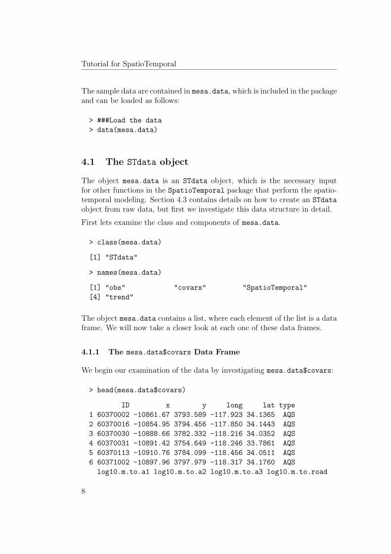
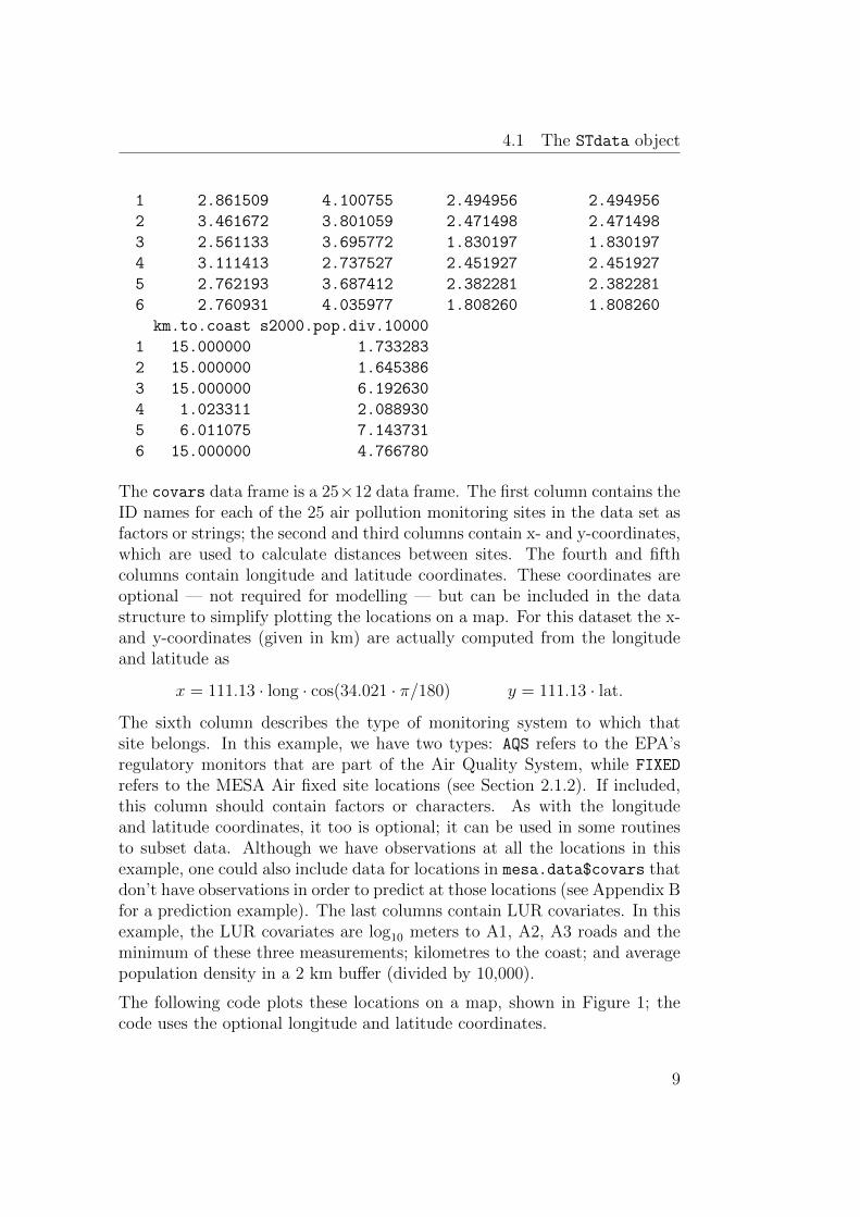
We begin our examination of the data by investigating mesa.data$covars:
> head(mesa.data$covars)
ID x y long lat type
1 60370002 -10861.67 3793.589 -117.923 34.1365 AQS
2 60370016 -10854.95 3794.456 -117.850 34.1443 AQS
3 60370030 -10888.66 3782.332 -118.216 34.0352 AQS
4 60370031 -10891.42 3754.649 -118.246 33.7861 AQS
5 60370113 -10910.76 3784.099 -118.456 34.0511 AQS
6 60371002 -10897.96 3797.979 -118.317 34.1760 AQS
log10.m.to.a1 log10.m.to.a2 log10.m.to.a3 log10.m.to.road
8
4.1 The STdata object
1 2.861509 4.100755 2.494956 2.494956
2 3.461672 3.801059 2.471498 2.471498
3 2.561133 3.695772 1.830197 1.830197
4 3.111413 2.737527 2.451927 2.451927
5 2.762193 3.687412 2.382281 2.382281
6 2.760931 4.035977 1.808260 1.808260
km.to.coast s2000.pop.div.10000
1 15.000000 1.733283
2 15.000000 1.645386
3 15.000000 6.192630
4 1.023311 2.088930
5 6.011075 7.143731
6 15.000000 4.766780
The covars data frame is a 25×12 data frame. The first column contains theID names for each of the 25 air pollution monitoring sites in the data set asfactors or strings; the second and third columns contain x- and y-coordinates,which are used to calculate distances between sites. The fourth and fifthcolumns contain longitude and latitude coordinates. These coordinates areoptional — not required for modelling — but can be included in the datastructure to simplify plotting the locations on a map. For this dataset the x-and y-coordinates (given in km) are actually computed from the longitudeand latitude as
x = 111.13 · long · cos(34.021 · π/180) y = 111.13 · lat.
The sixth column describes the type of monitoring system to which thatsite belongs. In this example, we have two types: AQS refers to the EPA’sregulatory monitors that are part of the Air Quality System, while FIXED
refers to the MESA Air fixed site locations (see Section 2.1.2). If included,this column should contain factors or characters. As with the longitudeand latitude coordinates, it too is optional; it can be used in some routinesto subset data. Although we have observations at all the locations in thisexample, one could also include data for locations in mesa.data$covars thatdon’t have observations in order to predict at those locations (see Appendix Bfor a prediction example). The last columns contain LUR covariates. In thisexample, the LUR covariates are log10 meters to A1, A2, A3 roads and theminimum of these three measurements; kilometres to the coast; and averagepopulation density in a 2 km buffer (divided by 10,000).
The following code plots these locations on a map, shown in Figure 1; thecode uses the optional longitude and latitude coordinates.
9

Tutorial for SpatioTemporal
> ###Plot the locations, see Figure 1
> par(mfrow=c(1,1))
> plot(mesa.data$covars$long, mesa.data$covars$lat,
pch=24, bg=c("red","blue")[mesa.data$covars$type],
xlab="Longitude", ylab="Latitude")
> ###Add the map of LA
> map("county", "california", col="#FFFF0055", fill=TRUE,
add=TRUE)
> ##Add a legend
> legend("bottomleft", c("AQS","FIXED"), pch=24, bty="n",
pt.bg=c("red","blue"))
−118.4 −118.2 −118.0 −117.8
33.7
33.8
33.9
34.0
34.1
34.2
Longitude
Latit
ude
AQSFIXED
Figure 1: Location of monitors in the Los Angeles area.
10

4.1 The STdata object
4.1.2 The mesa.data$trend Data Frame
Next, look at mesa.data$trend:
> head(mesa.data$trend)
V1 V2 date
1 -1.8591693 1.20721096 1999-01-13
2 -1.5200057 0.90473775 1999-01-27
3 -1.1880840 0.62679098 1999-02-10
4 -0.8639833 0.38411634 1999-02-24
5 -0.5536476 0.19683161 1999-03-10
6 -0.2643623 0.08739755 1999-03-24
The trend data frame consists of 2 smooth temporal basis functions com-puted using singular value decomposition (SVD), see Section 5 for details.These temporal trends corresponds to the fi(t):s in (2). The spatio-temporalmodel also includes an intercept, i.e. a vector of 1’s; the intercept is addedautomatically and should not be included in trend.
The mesa.data$trend data frame is 280 × 3, where 280 is the number oftime points for which we have NOx concentration measurements. Here,the first two columns contain smooth temporal trends, and the last columncontains dates in the R date format. In general, one of the columns inmesa.data$trend must be called date and have dates in the R date format;the names of the other columns are arbitrary. Studying the date component,
> range(mesa.data$trend$date)
[1] "1999-01-13" "2009-09-23"
we see that measurements are made over a period of about 10 years, fromJanuary 13, 1999 until September 23, 2009.
4.1.3 The mesa.data$obs Data Frame
The observations are stored in mesa.data$obs:
> head(mesa.data$obs)
11

Tutorial for SpatioTemporal
obs date ID
1 4.577684 1999-01-13 60370002
2 4.131632 1999-01-13 60370016
3 4.727882 1999-01-13 60370113
4 5.352608 1999-01-13 60371002
5 5.281452 1999-01-13 60371103
6 4.984585 1999-01-13 60371201
The data frame, mesa.data$obs, consists of observations, over time, for eachof the 25 locations. The data frame contains three variables: obs — themeasured log NOx concentrations (as 2-week averages); date — the date ofeach observation (here the middle Wednesday of each 2-week period); and ID
— labels indicating at which monitoring site each measurement was taken.Details regarding the monitoring can be found in Cohen et al. (2009), and abrief introduction is given in Section 2.1.
The ID values should correspond to the ID of the monitoring locations givenin mesa.data$location$ID. The dates in mesa.data$obs do not need tocorrespond exactly to the dates in mesa.data$trend$date; however theyhave to be in the range of mesa.data$trend$date (in this case, 1999-01-13through 2009-09-23).
Note that the number of rows in mesa.data$obs is 4577, far fewer than the280× 25 = 7000 observations there would be if each location had a completetime series of observations.
4.1.4 The mesa.data$SpatioTemporal Array
Finally, examine the mesa.data$SpatioTemporal data:
> dim(mesa.data$SpatioTemp)
[1] 280 25 1
> mesa.data$SpatioTemp[1:5,1:5,]
60370002 60370016 60370030 60370031 60370113
1999-01-13 2.3188 0 8.0641 0.1467 2.9894
1999-01-27 1.8371 0 7.3568 0.2397 4.7381
1999-02-10 1.4886 0 6.3673 0.2463 4.3922
1999-02-24 2.5868 0 7.1783 0.1140 3.3456
1999-03-10 1.8996 0 6.3159 0.1537 3.8495
12
4.1 The STdata object
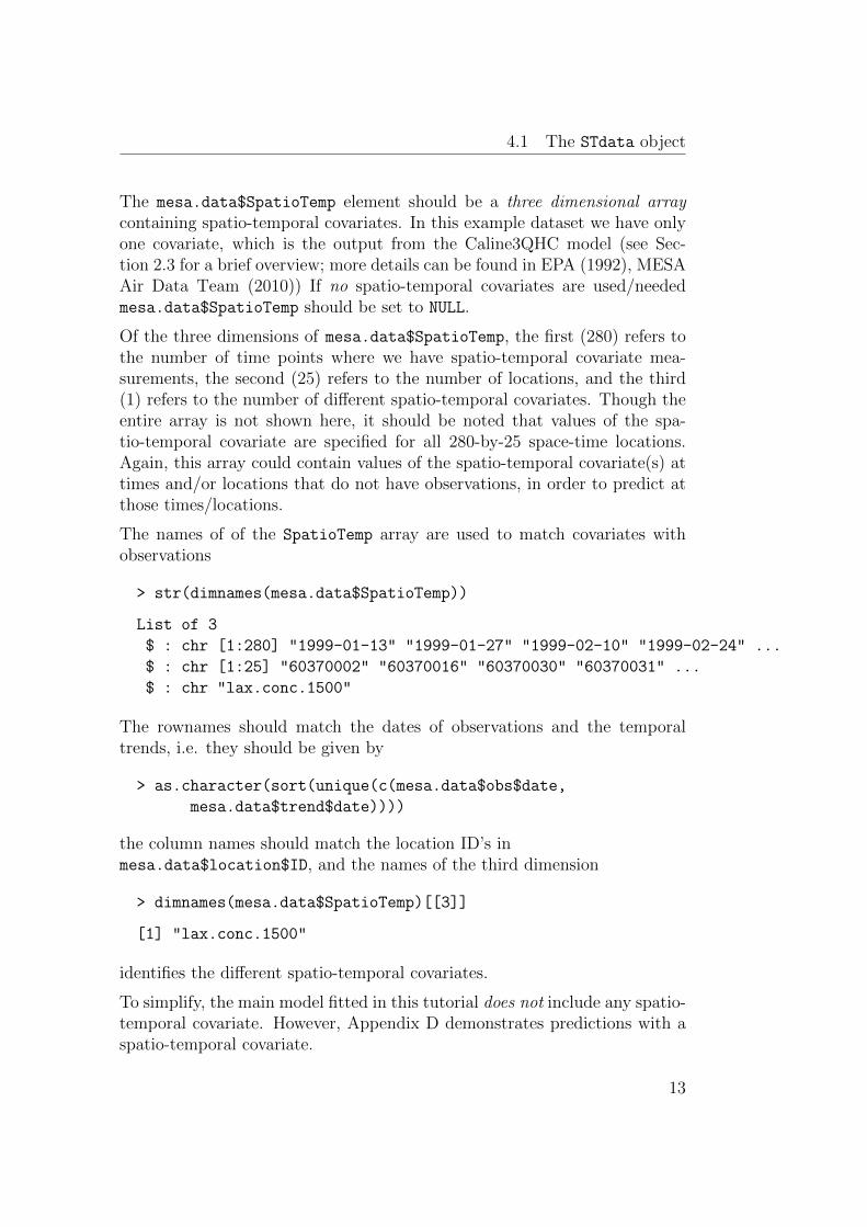
The mesa.data$SpatioTemp element should be a three dimensional arraycontaining spatio-temporal covariates. In this example dataset we have onlyone covariate, which is the output from the Caline3QHC model (see Sec-tion 2.3 for a brief overview; more details can be found in EPA (1992), MESAAir Data Team (2010)) If no spatio-temporal covariates are used/neededmesa.data$SpatioTemp should be set to NULL.
Of the three dimensions of mesa.data$SpatioTemp, the first (280) refers tothe number of time points where we have spatio-temporal covariate mea-surements, the second (25) refers to the number of locations, and the third(1) refers to the number of different spatio-temporal covariates. Though theentire array is not shown here, it should be noted that values of the spa-tio-temporal covariate are specified for all 280-by-25 space-time locations.Again, this array could contain values of the spatio-temporal covariate(s) attimes and/or locations that do not have observations, in order to predict atthose times/locations.
The names of of the SpatioTemp array are used to match covariates withobservations
> str(dimnames(mesa.data$SpatioTemp))
List of 3
$ : chr [1:280] "1999-01-13" "1999-01-27" "1999-02-10" "1999-02-24" ...
$ : chr [1:25] "60370002" "60370016" "60370030" "60370031" ...
$ : chr "lax.conc.1500"
The rownames should match the dates of observations and the temporaltrends, i.e. they should be given by
> as.character(sort(unique(c(mesa.data$obs$date,
mesa.data$trend$date))))
the column names should match the location ID’s inmesa.data$location$ID, and the names of the third dimension
> dimnames(mesa.data$SpatioTemp)[[3]]
[1] "lax.conc.1500"
identifies the different spatio-temporal covariates.
To simplify, the main model fitted in this tutorial does not include any spatio-temporal covariate. However, Appendix D demonstrates predictions with aspatio-temporal covariate.
13
Tutorial for SpatioTemporal
4.2 Summaries of mesa.data
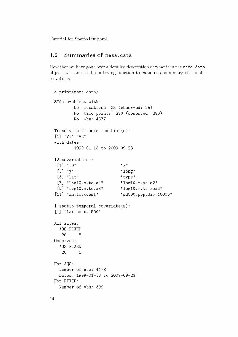
Now that we have gone over a detailed description of what is in the mesa.dataobject, we can use the following function to examine a summary of the ob-servations:
> print(mesa.data)
STdata-object with:
No. locations: 25 (observed: 25)
No. time points: 280 (observed: 280)
No. obs: 4577
Trend with 2 basis function(s):
[1] "V1" "V2"
with dates:
1999-01-13 to 2009-09-23
12 covariate(s):
[1] "ID" "x"
[3] "y" "long"
[5] "lat" "type"
[7] "log10.m.to.a1" "log10.m.to.a2"
[9] "log10.m.to.a3" "log10.m.to.road"
[11] "km.to.coast" "s2000.pop.div.10000"
1 spatio-temporal covariate(s):
[1] "lax.conc.1500"
All sites:
AQS FIXED
20 5
Observed:
AQS FIXED
20 5
For AQS:
Number of obs: 4178
Dates: 1999-01-13 to 2009-09-23
For FIXED:
Number of obs: 399
14

4.3 Creating an STdata object from raw data
Dates: 2005-12-07 to 2009-07-01
Here we can see the number of AQS and MESA FIXED sites in the mesa.datastructure. There are 20 AQS sites, which correspond to the number of loca-tions marked as AQS in mesa.data$covars$type, and 5 FIXED sites, whichcorrespond to the 5 sites flagged as FIXED inmesa.data$covars$type. We can also see that the observations are madeover the same range of time as the temporal trends; this is appropriate, asdiscussed above. The summary also indicates the total number of sites (andtime points) as well as how many of these that have been observed, Nbr lo-
cations: 25 (observed: 25). In this example all of our locations havebeen observed; Appendix B provides an example with unobserved locations.
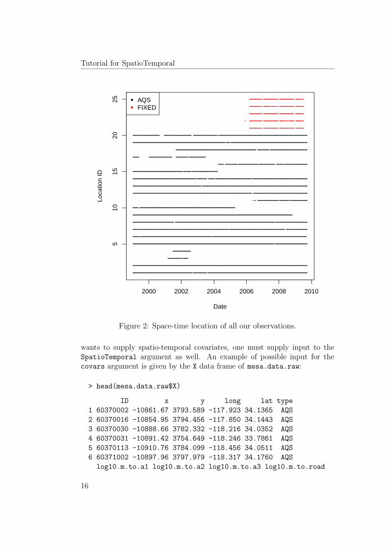
To graphically depict where and when our observation occurred we plot themonitor locations in time and space.
> ###Plot when observations occurr, see Figure 2
> par(mfcol=c(1,1),mar=c(4.3,4.3,1,1))
> plot(mesa.data, "loc")
From Figure 2 we see that the MESA monitors only sampled during thesecond half of the period. We also note that the number of observations varygreatly for different locations.
4.3 Creating an STdata object from raw data
Section 4.1 gave a detailed description of the STdata object. This sectiongives instructions for getting raw data into this format. The SpatioTemporalpackage contains an example of a raw data structure, which we now load andexamine.
> data(mesa.data.raw)
> names(mesa.data.raw)
[1] "X" "obs" "lax.conc.1500"
As we can see, the raw data contains a list of three data sets: "X", "obs",and "lax.conc.1500".
We will use the createSTdata() function to create the STdata object. ThecreateSTdata() function requires two arguments: obs and covars. If one
15
Tutorial for SpatioTemporal
2000 2002 2004 2006 2008 2010
510
1520
25
Date
Loca
tion
ID
●
●
●
●
●
●
●
●
●
●
●
●
●
●
●
●
●
●
●
●
●
●
●
●
●
●
●
●
●
●
●
●
●
●
●
●
●
●
●
●
●
●
●
●
●
●
●
●
●
●
●
●
●
●
●
●
●
●
●
●
●
●
●
●
●
●
●
●
●
●
●
●
●
●
●
●
●
●
●
●
●
●
●
●
●
●
●
●
●
●
●
●
●
●
●
●
●
●
●
●
●
●
●
●
●
●
●
●
●
●
●
●
●
●
●
●
●
●
●
●
●
●
●
●
●
●
●
●
●
●
●
●
●
●
●
●
●
●
●
●
●
●
●
●
●
●
●
●
●
●
●
●
●
●
●
●
●
●
●
●
●
●
●
●
●
●
●
●
●
●
●
●
●
●
●
●
●
●
●
●
●
●
●
●
●
●
●
●
●
●
●
●
●
●
●
●
●
●
●
●
●
●
●
●
●
●
●
●
●
●
●
●
●
●
●
●
●
●
●
●
●
●
●
●
●
●
●
●
●
●
●
●
●
●
●
●
●
●
●
●
●
●
●
●
●
●
●
●
●
●
●
●
●
●
●
●
●
●
●
●
●
●
●
●
●
●
●
●
●
●
●
●
●
●
●
●
●
●
●
●
●
●
●
●
●
●
●
●
●
●
●
●
●
●
●
●
●
●
●
●
●
●
●
●
●
●
●
●
●
●
●
●
●
●
●
●
●
●
●
●
●
●
●
●
●
●
●
●
●
●
●
●
●
●
●
●
●
●
●
●
●
●
●
●
●
●
●
●
●
●
●
●
●
●
●
●
●
●
●
●
●
●
●
●
●
●
●
●
●
●
●
●
●
●
●
●
●
●
●
●
●
●
●
●
●
●
●
●
●
●
●
●
●
●
●
●
●
●
●
●
●
●
●
●
●
●
●
●
●
●
●
●
●
●
●
●
●
●
●
●
●
●
●
●
●
●
●
●
●
●
●
●
●
●
●
●
●
●
●
●
●
●
●
●
●
●
●
●
●
●
●
●
●
●
●
●
●
●
●
●
●
●
●
●
●
●
●
●
●
●
●
●
●
●
●
●
●
●
●
●
●
●
●
●
●
●
●
●
●
●
●
●
●
●
●
●
●
●
●
●
●
●
●
●
●
●
●
●
●
●
●
●
●
●
●
●
●
●
●
●
●
●
●
●
●
●
●
●
●
●
●
●
●
●
●
●
●
●
●
●
●
●
●
●
●
●
●
●
●
●
●
●
●
●
●
●
●
●
●
●
●
●
●
●
●
●
●
●
●
●
●
●
●
●
●
●
●
●
●
●
●
●
●
●
●
●
●
●
●
●
●
●
●
●
●
●
●
●
●
●
●
●
●
●
●
●
●
●
●
●
●
●
●
●
●
●
●
●
●
●
●
●
●
●
●
●
●
●
●
●
●
●
●
●
●
●
●
●
●
●
●
●
●
●
●
●
●
●
●
●
●
●
●
●
●
●
●
●
●
●
●
●
●
●
●
●
●
●
●
●
●
●
●
●
●
●
●
●
●
●
●
●
●
●
●
●
●
●
●
●
●
●
●
●
●
●
●
●
●
●
●
●
●
●
●
●
●
●
●
●
●
●
●
●
●
●
●
●
●
●
●
●
●
●
●
●
●
●
●
●
●
●
●
●
●
●
●
●
●
●
●
●
●
●
●
●
●
●
●
●
●
●
●
●
●
●
●
●
●
●
●
●
●
●
●
●
●
●
●
●
●
●
●
●
●
●
●
●
●
●
●
●
●
●
●
●
●
●
●
●
●
●
●
●
●
●
●
●
●
●
●
●
●
●
●
●
●
●
●
●
●
●
●
●
●
●
●
●
●
●
●
●
●
●
●
●
●
●
●
●
●
●
●
●
●
●
●
●
●
●
●
●
●
●
●
●
●
●
●
●
●
●
●
●
●
●
●
●
●
●
●
●
●
●
●
●
●
●
●
●
●
●
●
●
●
●
●
●
●
●
●
●
●
●
●
●
●
●
●
●
●
●
●
●
●
●
●
●
●
●
●
●
●
●
●
●
●
●
●
●
●
●
●
●
●
●
●
●
●
●
●
●
●
●
●
●
●
●
●
●
●
●
●
●
●
●
●
●
●
●
●
●
●
●
●
●
●
●
●
●
●
●
●
●
●
●
●
●
●
●
●
●
●
●
●
●
●
●
●
●
●
●
●
●
●
●
●
●
●
●
●
●
●
●
●
●
●
●
●
●
●
●
●
●
●
●
●
●
●
●
●
●
●
●
●
●
●
●
●
●
●
●
●
●
●
●
●
●
●
●
●
●
●
●
●
●
●
●
●
●
●
●
●
●
●
●
●
●
●
●
●
●
●
●
●
●
●
●
●
●
●
●
●
●
●
●
●
●
●
●
●
●
●
●
●
●
●
●
●
●
●
●
●
●
●
●
●
●
●
●
●
●
●
●
●
●
●
●
●
●
●
●
●
●
●
●
●
●
●
●
●
●
●
●
●
●
●
●
●
●
●
●
●
●
●
●
●
●
●
●
●
●
●
●
●
●
●
●
●
●
●
●
●
●
●
●
●
●
●
●
●
●
●
●
●
●
●
●
●
●
●
●
●
●
●
●
●
●
●
●
●
●
●
●
●
●
●
●
●
●
●
●
●
●
●
●
●
●
●
●
●
●
●
●
●
●
●
●
●
●
●
●
●
●
●
●
●
●
●
●
●
●
●
●
●
●
●
●
●
●
●
●
●
●
●
●
●
●
●
●
●
●
●
●
●
●
●
●
●
●
●
●
●
●
●
●
●
●
●
●
●
●
●
●
●
●
●
●
●
●
●
●
●
●
●
●
●
●
●
●
●
●
●
●
●
●
●
●
●
●
●
●
●
●
●
●
●
●
●
●
●
●
●
●
●
●
●
●
●
●
●
●
●
●
●
●
●
●
●
●
●
●
●
●
●
●
●
●
●
●
●
●
●
●
●
●
●
●
●
●
●
●
●
●
●
●
●
●
●
●
●
●
●
●
●
●
●
●
●
●
●
●
●
●
●
●
●
●
●
●
●
●
●
●
●
●
●
●
●
●
●
●
●
●
●
●
●
●
●
●
●
●
●
●
●
●
●
●
●
●
●
●
●
●
●
●
●
●
●
●
●
●
●
●
●
●
●
●
●
●
●
●
●
●
●
●
●
●
●
●
●
●
●
●
●
●
●
●
●
●
●
●
●
●
●
●
●
●
●
●
●
●
●
●
●
●
●
●
●
●
●
●
●
●
●
●
●
●
●
●
●
●
●
●
●
●
●
●
●
●
●
●
●
●
●
●
●
●
●
●
●
●
●
●
●
●
●
●
●
●
●
●
●
●
●
●
●
●
●
●
●
●
●
●
●
●
●
●
●
●
●
●
●
●
●
●
●
●
●
●
●
●
●
●
●
●
●
●
●
●
●
●
●
●
●
●
●
●
●
●
●
●
●
●
●
●
●
●
●
●
●
●
●
●
●
●
●
●
●
●
●
●
●
●
●
●
●
●
●
●
●
●
●
●
●
●
●
●
●
●
●
●
●
●
●
●
●
●
●
●
●
●
●
●
●
●
●
●
●
●
●
●
●
●
●
●
●
●
●
●
●
●
●
●
●
●
●
●
●
●
●
●
●
●
●
●
●
●
●
●
●
●
●
●
●
●
●
●
●
●
●
●
●
●
●
●
●
●
●
●
●
●
●
●
●
●
●
●
●
●
●
●
●
●
●
●
●
●
●
●
●
●
●
●
●
●
●
●
●
●
●
●
●
●
●
●
●
●
●
●
●
●
●
●
●
●
●
●
●
●
●
●
●
●
●
●
●
●
●
●
●
●
●
●
●
●
●
●
●
●
●
●
●
●
●
●
●
●
●
●
●
●
●
●
●
●
●
●
●
●
●
●
●
●
●
●
●
●
●
●
●
●
●
●
●
●
●
●
●
●
●
●
●
●
●
●
●
●
●
●
●
●
●
●
●
●
●
●
●
●
●
●
●
●
●
●
●
●
●
●
●
●
●
●
●
●
●
●
●
●
●
●
●
●
●
●
●
●
●
●
●
●
●
●
●
●
●
●
●
●
●
●
●
●
●
●
●
●
●
●
●
●
●
●
●
●
●
●
●
●
●
●
●
●
●
●
●
●
●
●
●
●
●
●
●
●
●
●
●
●
●
●
●
●
●
●
●
●
●
●
●
●
●
●
●
●
●
●
●
●
●
●
●
●
●
●
●
●
●
●
●
●
●
●
●
●
●
●
●
●
●
●
●
●
●
●
●
●
●
●
●
●
●
●
●
●
●
●
●
●
●
●
●
●
●
●
●
●
●
●
●
●
●
●
●
●
●
●
●
●
●
●
●
●
●
●
●
●
●
●
●
●
●
●
●
●
●
●
●
●
●
●
●
●
●
●
●
●
●
●
●
●
●
●
●
●
●
●
●
●
●
●
●
●
●
●
●
●
●
●
●
●
●
●
●
●
●
●
●
●
●
●
●
●
●
●
●
●
●
●
●
●
●
●
●
●
●
●
●
●
●
●
●
●
●
●
●
●
●
●
●
●
●
●
●
●
●
●
●
●
●
●
●
●
●
●
●
●
●
●
●
●
●
●
●
●
●
●
●
●
●
●
●
●
●
●
●
●
●
●
●
●
●
●
●
●
●
●
●
●
●
●
●
●
●
●
●
●
●
●
●
●
●
●
●
●
●
●
●
●
●
●
●
●
●
●
●
●
●
●
●
●
●
●
●
●
●
●
●
●
●
●
●
●
●
●
●
●
●
●
●
●
●
●
●
●
●
●
●
●
●
●
●
●
●
●
●
●
●
●
●
●
●
●
●
●
●
●
●
●
●
●
●
●
●
●
●
●
●
●
●
●
●
●
●
●
●
●
●
●
●
●
●
●
●
●
●
●
●
●
●
●
●
●
●
●
●
●
●
●
●
●
●
●
●
●
●
●
●
●
●
●
●
●
●
●
●
●
●
●
●
●
●
●
●
●
●
●
●
●
●
●
●
●
●
●
●
●
●
●
●
●
●
●
●
●
●
●
●
●
●
●
●
●
●
●
●
●
●
●
●
●
●
●
●
●
●
●
●
●
●
●
●
●
●
●
●
●
●
●
●
●
●
●
●
●
●
●
●
●
●
●
●
●
●
●
●
●
●
●
●
●
●
●
●
●
●
●
●
●
●
●
●
●
●
●
●
●
●
●
●
●
●
●
●
●
●
●
●
●
●
●
●
●
●
●
●
●
●
●
●
●
●
●
●
●
●
●
●
●
●
●
●
●
●
●
●
●
●
●
●
●
●
●
●
●
●
●
●
●
●
●
●
●
●
●
●
●
●
●
●
●
●
●
●
●
●
●
●
●
●
●
●
●
●
●
●
●
●
●
●
●
●
●
●
●
●
●
●
●
●
●
●
●
●
●
●
●
●
●
●
●
●
●
●
●
●
●
●
●
●
●
●
●
●
●
●
●
●
●
●
●
●
●
●
●
●
●
●
●
●
●
●
●
●
●
●
●
●
●
●
●
●
●
●
●
●
●
●
●
●
●
●
●
●
●
●
●
●
●
●
●
●
●
●
●
●
●
●
●
●
●
●
●
●
●
●
●
●
●
●
●
●
●
●
●
●
●
●
●
●
●
●
●
●
●
●
●
●
●
●
●
●
●
●
●
●
●
●
●
●
●
●
●
●
●
●
●
●
●
●
●
●
●
●
●
●
●
●
●
●
●
●
●
●
●
●
●
●
●
●
●
●
●
●
●
●
●
●
●
●
●
●
●
●
●
●
●
●
●
●
●
●
●
●
●
●
●
●
●
●
●
●
●
●
●
●
●
●
●
●
●
●
●
●
●
●
●
●
●
●
●
●
●
●
●
●
●
●
●
●
●
●
●
●
●
●
●
●
●
●
●
●
●
●
●
●
●
●
●
●
●
●
●
●
●
●
●
●
●
●
●
●
●
●
●
●
●
●
●
●
●
●
●
●
●
●
●
●
●
●
●
●
●
●
●
●
●
●
●
●
●
●
●
●
●
●
●
●
●
●
●
●
●
●
●
●
●
●
●
●
●
●
●
●
●
●
●
●
●
●
●
●
●
●
●
●
●
●
●
●
●
●
●
●
●
●
●
●
●
●
●
●
●
●
●
●
●
●
●
●
●
●
●
●
●
●
●
●
●
●
●
●
●
●
●
●
●
●
●
●
●
●
●
●
●
●
●
●
●
●
●
●
●
●
●
●
●
●
●
●
●
●
●
●
●
●
●
●
●
●
●
●
●
●
●
●
●
●
●
●
●
●
●
●
●
●
●
●
●
●
●
●
●
●
●
●
●
●
●
●
●
●
●
●
●
●
●
●
●
●
●
●
●
●
●
●
●
●
●
●
●
●
●
●
●
●
●
●
●
●
●
●
●
●
●
●
●
●
●
●
●
●
●
●
●
●
●
●
●
●
●
●
●
●
●
●
●
●
●
●
●
●
●
●
●
●
●
●
●
●
●
●
●
●
●
●
●
●
●
●
●
●
●
●
●
●
●
●
●
●
●
●
●
●
●
●
●
●
●
●
●
●
●
●
●
●
●
●
●
●
●
●
●
●
●
●
●
●
●
●
●
●
●
●
●
●
●
●
●
●
●
●
●
●
●
●
●
●
●
●
●
●
●
●
●
●
●
●
●
●
●
●
●
●
●
●
●
●
●
●
●
●
●
●
●
●
●
●
●
●
●
●
●
●
●
●
●
●
●
●
●
●
●
●
●
●
●
●
●
●
●
●
●
●
●
●
●
●
●
●
●
●
●
●
●
●
●
●
●
●
●
●
●
●
●
●
●
●
●
●
●
●
●
●
●
●
●
●
●
●
●
●
●
●
●
●
●
●
●
●
●
●
●
●
●
●
●
●
●
●
●
●
●
●
●
●
●
●
●
●
●
●
●
●
●
●
●
●
●
●
●
●
●
●
●
●
●
●
●
●
●
●
●
●
●
●
●
●
●
●
●
●
●
●
●
●
●
●
●
●
●
●
●
●
●
●
●
●
●
●
●
●
●
●
●
●
●
●
●
●
●
●
●
●
●
●
●
●
●
●
●
●
●
●
●
●
●
●
●
●
●
●
●
●
●
●
●
●
●
●
●
●
●
●
●
●
●
●
●
●
●
●
●
●
●
●
●
●
●
●
●
●
●
●
●
●
●
●
●
●
●
●
●
●
●
●
●
●
●
●
●
●
●
●
●
●
●
●
●
●
●
●
●
●
●
●
●
●
●
●
●
●
●
●
●
●
●
●
●
●
●
●
●
●
●
●
●
●
●
●
●
●
●
●
●
●
●
●
●
●
●
●
●
●
●
●
●
●
●
●
●
●
●
●
●
●
●
●
●
●
●
●
●
●
●
●
●
●
●
●
●
●
●
●
●
●
●
●
●
●
●
●
●
●
●
●
●
●
●
●
●
●
●
●
●
●
●
●
●
●
●
●
●
●
●
●
●
●
●
●
●
●
●
●
●
●
●
●
●
●
●
●
●
●
●
●
●
●
●
●
●
●
●
●
●
●
●
●
●
●
●
●
●
●
●
●
●
●
●
●
●
●
●
●
●
●
●
●
●
●
●
●
●
●
●
●
●
●
●
●
●
●
●
●
●
●
●
●
●
●
●
●
●
●
●
●
●
●
●
●
●
●
●
●
●
●
●
●
●
●
●
●
●
●
●
●
●
●
●
●
●
●
●
●
●
●
●
●
●
●
●
●
●
●
●
●
●
●
●
●
●
●
●
●
●
●
●
●
●
●
●
●
●
●
●
●
●
●
●
●
●
●
●
●
●
●
●
●
●
●
●
●
●
●
●
●
●
●
●
●
●
●
●
●
●
●
●
●
●
●
●
●
●
●
●
●
●
●
●
●
●
●
●
●
●
●
●
●
●
●
●
●
●
●
●
●
●
●
●
●
●
●
●
●
●
●
●
●
●
●
●
●
●
●
●
●
●
●
●
●
●
●
●
●
●
●
●
●
●
●
●
●
●
●
●
●
●
●
●
●
●
●
●
●
●
●
●
●
●
●
●
●
●
●
●
●
●
●
●
●
●
●
●
●
●
●
●
●
●
●
●
●
●
●
●
●
●
●
●
●
●
●
●
●
●
●
●
●
●
●
●
●
●
●
●
●
●
●
●
●
●
●
●
●
●
●
●
●
●
●
●
●
●
●
●
●
●
●
●
●
●
●
●
●
●
●
●
●
●
●
●
●
●
●
●
●
●
●
●
●
●
●
●
●
●
●
●
●
●
●
●
●
●
●
●
●
●
●
●
●
●
●
●
●
●
●
●
●
●
●
●
●
●
●
●
●
●
●
●
●
●
●
●
●
●
●
●
●
●
●
●
●
●
●
●
●
●
●
●
●
●
●
●
●
●
●
●
●
●
●
●
●
●
●
●
●
●
●
●
●
●
●
●
●
●
●
●
●
●
●
●
●
●
●
●
●
●
●
●
●
●
●
●
●
●
●
●
●
●
●
●
●
●
●
●
●
●
●
●
●
●
●
●
●
●
●
●
●
●
●
●
●
●
●
●
●
●
●
●
●
●
●
●
●
●
●
●
●
●
●
●
●
●
●
●
●
●
●
●
●
●
●
●
●
●
●
●
●
●
●
●
●
●
●
●
●
●
●
●
●
●
●
●
●
●
●
●
●
●
●
●
●
●
●
●
●
●
●
●
●
●
●
●
●
●
●
●
●
●
●
●
●
●
●
●
●
●
●
●
●
●
●
●
●
●
●
●
●
●
●
●
●
●
●
●
●
●
●
●
●
●
●
●
●
●
●
●
●
●
●
●
●
●
●
●
●
●
●
●
●
●
●
●
●
●
●
●
●
●
●
●
●
●
●
●
●
●
●
●
●
●
●
●
●
●
●
●
●
●
●
●
●
●
●
●
●
●
●
●
●
●
●
●
●
●
●
●
●
●
●
●
●
●
●
●
●
●
●
●
●
●
●
●
●
●
●
●
●
●
●
●
●
●
●
●
●
●
●
●
●
●
●
●
●
●
●
●
●
●
●
●
●
●
●
●
●
●
●
●
●
●
●
●
●
●
●
●
●
●
●
●
●
●
●
●
●
●
●
●
●
●
●
●
●
●
●
●
●
●
●
●
●
●
●
●
●
●
●
●
●
●
●
●
●
●
●
●
●
●
●
●
●
●
●
●
●
●
●
●
●
●
●
●
●
●
●
●
●
●
●
●
●
●
●
●
●
●
●
●
●
●
●
●
●
●
●
●
●
●
●
●
●
●
●
●
●
●
●
●
●
●
●
●
●
●
●
●
●
●
●
●
●
●
●
●
●
●
●
●
●
●
●
●
●
●
●
●
●
●
●
●
●
●
●
●
●
●
●
●
●
●
●
●
●
●
●
●
●
●
●
●
●
●
●
●
●
●
●
●
●
●
●
●
●
●
●
●
●
●
●
●
●
●
●
●
●
●
●
●
●
●
●
●
●
●
●
●
●
●
●
●
●
●
●
●
●
●
●
●
●
●
●
●
●
●
●
●
●
●
●
●
●
●
●
●
●
●
●
●
●
●
●
●
●
●
●
●
●
●
●
●
●
●
●
●
●
●
●
●
●
●
●
●
●
●
●
●
●
●
●
●
●
●
●
●
●
●
●
●
●
●
●
●
●
●
●
●
●
●
●
●
●
●
●
●
●
●
●
●
●
●
●
●
●
●
●
●
●
●
●
●
●
●
●
●
●
●
●
●
●
●
●
●
●
●
●
●
●
●
●
●
●
●
●
●
●
●
●
●
●
●
●
●
●
●
●
●
●
●
●
●
●
●
●
●
●
●
●
●
●
●
●
●
●
●
●
●
●
●
●
●
●
●
●
●
●
●
●
●
●
●
●
●
●
●
●
●
●
●
●
●
●
●
●
●
●
●
●
●
●
●
●
●
●
●
●
●
●
●
●
●
●
●
●
●
●
●
●
●
●
●
●
●
●
●
●
●
●
●
●
●
●
●
●
●
●
●
●
●
●
●
●
●
●
●
●
●
●
●
●
●
●
●
●
●
●
●
●
●
●
●
●
●
●
●
●
●
●
●
●
●
●
●
●
●
●
●
●
●
●
●
●
●
●
●
●
●
●
●
●
●
●
●
●
●
●
●
●
●
●
●
●
●
●
●
●
●
●
●
●
●
●
●
●
●
●
●
●
●
●
●
●
●
●
●
●
●
●
●
●
●
●
●
●
●
●
●
●
●
●
●
●
●
●
●
●
●
●
●
●
●
●
●
●
●
●
●
●
●
●
●
●
●
●
●
●
●
●
●
●
●
●
●
●
●
●
●
●
AQSFIXED
Figure 2: Space-time location of all our observations.
wants to supply spatio-temporal covariates, one must supply input to theSpatioTemporal argument as well. An example of possible input for thecovars argument is given by the X data frame of mesa.data.raw:
> head(mesa.data.raw$X)
ID x y long lat type
1 60370002 -10861.67 3793.589 -117.923 34.1365 AQS
2 60370016 -10854.95 3794.456 -117.850 34.1443 AQS
3 60370030 -10888.66 3782.332 -118.216 34.0352 AQS
4 60370031 -10891.42 3754.649 -118.246 33.7861 AQS
5 60370113 -10910.76 3784.099 -118.456 34.0511 AQS
6 60371002 -10897.96 3797.979 -118.317 34.1760 AQS
log10.m.to.a1 log10.m.to.a2 log10.m.to.a3 log10.m.to.road
16

4.3 Creating an STdata object from raw data
1 2.861509 4.100755 2.494956 2.494956
2 3.461672 3.801059 2.471498 2.471498
3 2.561133 3.695772 1.830197 1.830197
4 3.111413 2.737527 2.451927 2.451927
5 2.762193 3.687412 2.382281 2.382281
6 2.760931 4.035977 1.808260 1.808260
km.to.coast s2000.pop.div.10000
1 15.000000 1.733283
2 15.000000 1.645386
3 15.000000 6.192630
4 1.023311 2.088930
5 6.011075 7.143731
6 15.000000 4.766780
Above we can see an excerpt of mesa.data.raw$X. In this example,mesa.data.raw$X contains information about the monitoring locations, in-cluding: names (or ID’s), x- and y-coordinates, and covariates from a GIS tobe used in the LUR. It also includes latitudes and longitudes, and monitortype. To satisfy the covars argument of createSTdata(), this data framerequires, at the minimum, coordinates, LUR covariates, and and ID column.The latitude and longitude, as well as the monitor type, are optional columns.
Next, examine the $obs part of the raw data.
> mesa.data.raw$obs[1:6,1:5]
60370002 60370016 60370030 60370031 60370113
1999-01-13 4.577684 4.131632 NA NA 4.727882
1999-01-27 3.889091 3.543566 NA NA 4.139332
1999-02-10 4.013020 3.632424 NA NA 4.054051
1999-02-24 4.080691 3.842586 NA NA 4.392799
1999-03-10 3.728085 3.396944 NA NA 3.960577
1999-03-24 3.751913 3.626161 NA NA 3.958741
In this example the observations are stored as a (number of time-points)-by-(number of locations) matrix with missing observations denote by NA,the row- and columnames identify the location and time point of each ob-servation. Alternatively, one could have the observations as a data framewith three columns: date, location ID and observations. This format ofmesa.data.raw$obs is more likely for data with only a few missing observa-tions.
17

Tutorial for SpatioTemporal
The final element is a spatio-temporal covariate, i.e. the output from theCaline3QHC model (see Section 2.3),
> mesa.data.raw$lax.conc.1500[1:6,1:5]
60370002 60370016 60370030 60370031 60370113
1999-01-13 2.3188 0 8.0641 0.1467 2.9894
1999-01-27 1.8371 0 7.3568 0.2397 4.7381
1999-02-10 1.4886 0 6.3673 0.2463 4.3922
1999-02-24 2.5868 0 7.1783 0.1140 3.3456
1999-03-10 1.8996 0 6.3159 0.1537 3.8495
1999-03-24 2.0162 0 6.3277 0.1906 3.2170
This matrix contains spatio-temporal covariate values for all locations andtimes. Similar to the mesa.data.raw$obs matrix, the row- and columnnames of the mesa.data.raw$lax.conc.1500 matrix contain the dates andlocation ID’s of the spatio-temporal covariate.
The measurement locations, LUR information, observations and spatio-tem-poral covariates (optional) above constitute the basic raw data needed bythe createSTdata() function. Given these minimal elements, creation ofthe STdata structure is easy:
> obs <- mesa.data.raw$obs
> covars <- mesa.data.raw$X
> ##list with the spatio-temporal covariates
> ST.list <- list(lax.conc.1500=mesa.data.raw$lax.conc.1500)
> ##create STdata object
> mesa.data.scratch <- createSTdata(obs, covars,
SpatioTemporal=ST.list,n.basis=2)
> names(mesa.data.scratch)
[1] "obs" "covars" "SpatioTemporal"
[4] "trend"
A few things to note here: we must first convert the mesa.data.raw$lax.conc.1500spatio-temporal covariate matrix to a list; the length of this list equals thenumber of spatio-temporal covariates we want to use (in this case, just 1).We also specified n.basis=2, which indicates we want to compute 2 temporaltrends: these will then be included in the mesa.data$trend object we sawin the previous section. If we leave this argument unspecified, no temporaltrends will be computed.
18

5. Estimating the Smooth Temporal Trends
Finally, make sure we created the right object:
> class(mesa.data.scratch)
[1] "STdata"
...and we’re good!
5 Estimating the Smooth Temporal Trends
The first step in analysing the data is to determine, using cross-validation,how many smooth temporal trends we need to capture the seasonal variabil-ity.
5.1 Data Set-Up for Trend Estimation
In order to estimate the smooth trends, we need a data matrix that is (numberof time-points)-by-(number of locations) in dimension. Here, the dimensionsrefer to time-points and locations where we have observations. Since ourmesa.data$obs data frame has a single column for the dates, locations, andobservations, we use the createDataMatrix() function to get the data intothe format needed for trend estimation:
> ##extract a data matrix
> D <- createDataMatrix(mesa.data)
> ##and study the data
> dim(D)
[1] 280 25
> D[1:6,1:5]
60370002 60370016 60370030 60370031 60370113
1999-01-13 4.577684 4.131632 NA NA 4.727882
1999-01-27 3.889091 3.543566 NA NA 4.139332
1999-02-10 4.013020 3.632424 NA NA 4.054051
1999-02-24 4.080691 3.842586 NA NA 4.392799
1999-03-10 3.728085 3.396944 NA NA 3.960577
1999-03-24 3.751913 3.626161 NA NA 3.958741
> colnames(D)
19

Tutorial for SpatioTemporal
[1] "60370002" "60370016" "60370030" "60370031" "60370113"
[6] "60371002" "60371103" "60371201" "60371301" "60371601"
[11] "60371602" "60371701" "60372005" "60374002" "60375001"
[16] "60375005" "60590001" "60590007" "60591003" "60595001"
[21] "L001" "L002" "LC001" "LC002" "LC003"
D is now a 280×25 matrix where each column represents observations at onelocation, and the rows represents points in time. Note that we supplied thecreateDataMatrix() function with an STdata object; alternatively we couldsupply the arguments obs, date, and ID individually. The matrix elementsmarked as NA indicate that there are no observation for those locations andtimes.
As a brief aside, note that we can also subset locations in thecreateDataMatrix() function. As an example, we create a data matrix foronly the AQS monitoring locations:
> ##subset the data
> ID.subset <-mesa.data$covars[mesa.data$covars$type ==
"AQS",]$ID
> D2 <- createDataMatrix(mesa.data, subset=ID.subset)
> ##and study the result
> dim(D2)
[1] 280 20
> colnames(D2)
[1] "60370002" "60370016" "60370030" "60370031" "60370113"
[6] "60371002" "60371103" "60371201" "60371301" "60371601"
[11] "60371602" "60371701" "60372005" "60374002" "60375001"
[16] "60375005" "60590001" "60590007" "60591003" "60595001"
Note that D2 is now a 280 × 20 matrix: we have created a data matrix foronly the AQS locations, dropping the 5 Mesa FIXED locations.
5.2 Cross-Validated Trend Estimations
The displayed portion of the data matrix D shows what we have already seenin Figure 2: not every location has a complete time series, and the times atwhich observations are made are not consistent across location. When de-termining the best number of smooth temporal trends and computing these
20

5.2 Cross-Validated Trend Estimations
trends we need to address the missing data. Fuentes et al. (2006) outlinesa procedure for computing smooth temporal trends from incomplete datamatrices, a brief description is given in Sections 5.2.1–5.2.3 below. The pro-cedure, including a cross validation to determine the best number of trends,is implemented by calling:
> ##Run leave one out cross-validation to find smooth trends
> SVD.cv <- SVDsmoothCV(D,1:5)
The function SVDsmoothCV performs a sequence of procedures, the end goalof which is to assist the user in choosing the optimal number of smoothtemporal trends that describe the seasonal variations in the data.SVDsmoothCV relies on two other functions: SVDmiss, that completes thedata matrix, and SVDsmooth, that computes smooth temporal trends fromthe completed data matrix. In this example, we will evaluate 1 through 5smooth trends in each, as specified by 1:5 in SVDsmoothCV(D,1:5).
To clarify: It is important to understand that the following procedures(filling in the data matrix, finding the m smooth temporal trends, andrunning the leave one out cross-validation) are done for each of the valuesm = (1, 2, . . . , 5).
5.2.1 SVDmiss: Completing the Data Matrix
The function SVDmiss completes a data matrix by iterating over the followingsteps (See Fuentes et al., 2006, for details.):
Step 0. Regression through the origin of the columns of the data matrix D (withthe NA’s replaced by zeroes) on a length 280 vector, u1, consisting ofthe mean concentration at each time point taken across all locationsthat are not NA. The missing observations are then replaced by the fittedvalues of that regression. For example, D[i,j] would be replaced bymultiplying the ith element of u1 with the regression coefficient obtainedby regressing the jth column of [D] on u1; missing values are ignoredin the regression.
For this step to be well defined the data matrix must have at least oneobservation in each row and column.
Step 1. Compute the SVD of the new data matrix with the missing valuesimputed.
21

Tutorial for SpatioTemporal
Step 2. Do regression of each column of the new data matrix on the first morthogonal basis functions found in Step 1. The missing values arethen replaced by the fitted values of this regression.
Step 3. Repeat from Step 1 until convergence; convergence being measured bythe change in the imputed values between iterations.
5.2.2 SVDsmooth: Smoothing
To obtain m smooth temporal trends, SVDsmooth first standardises the datamatrix so that each column is mean zero and variance one. The functionthen uses SVDmiss to complete the data matrix. Finally the function usessmooth.spline to smooth the m first orthogonal basis functions of the com-peted data matrix; as computed by SVDmiss.
5.2.3 SVDsmoothCV: Cross-Validating
Finally, the function SVDsmoothCV does leave-one-column-out (i.e. leave-one-site-out) cross-validation, and computes cross-validated statistics. Thesestatistics are given in order to provide user guidance in choosing the numberof temporal trends that are needed to describe the seasonal variations. Thecross-validation procedure is carried out thus:
1. Leave out one column of D, call the reduced matrix D
2. Impute the missing values and obtain m smooth temporal trends for Dby calling SVDsmooth.
3. Do regression of the left-out column of D on the set of m smooth ba-sis functions; use the residuals from the regression to compute cross-validation statistics
An important thing to keep in mind is that the value of m is fixed acrossthe functions that are calling each other. That is, SVDsmoothCV first does across-validation for m=1 (and hence calls SVDsmooth with m = 1, which callsSVDmiss with m=1) and calculates cross-validation statistics; then it does anew cross-validation for m = 2 (which in turn calls SVDsmooth with m = 2,etc.). From the output we can then compare the cross-validation statisticsfor each of the 5 sets of cross-validations (where m goes from 1 to 5.)
22
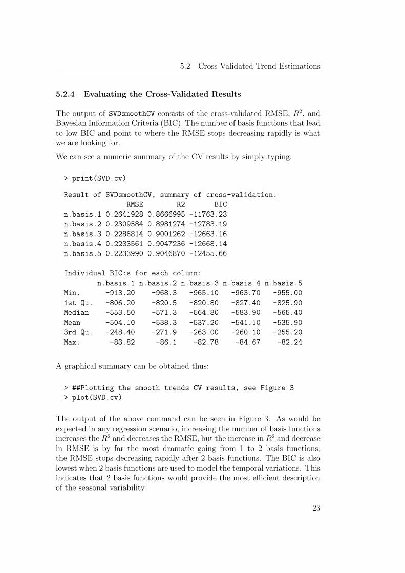
5.2 Cross-Validated Trend Estimations
5.2.4 Evaluating the Cross-Validated Results
The output of SVDsmoothCV consists of the cross-validated RMSE, R2, andBayesian Information Criteria (BIC). The number of basis functions that leadto low BIC and point to where the RMSE stops decreasing rapidly is whatwe are looking for.
We can see a numeric summary of the CV results by simply typing:
> print(SVD.cv)
Result of SVDsmoothCV, summary of cross-validation:
RMSE R2 BIC
n.basis.1 0.2641928 0.8666995 -11763.23
n.basis.2 0.2309584 0.8981274 -12783.19
n.basis.3 0.2286814 0.9001262 -12663.16
n.basis.4 0.2233561 0.9047236 -12668.14
n.basis.5 0.2233990 0.9046870 -12455.66
Individual BIC:s for each column:
n.basis.1 n.basis.2 n.basis.3 n.basis.4 n.basis.5
Min. -913.20 -968.3 -965.10 -963.70 -955.00
1st Qu. -806.20 -820.5 -820.80 -827.40 -825.90
Median -553.50 -571.3 -564.80 -583.90 -565.40
Mean -504.10 -538.3 -537.20 -541.10 -535.90
3rd Qu. -248.40 -271.9 -263.00 -260.10 -255.20
Max. -83.82 -86.1 -82.78 -84.67 -82.24
A graphical summary can be obtained thus:
> ##Plotting the smooth trends CV results, see Figure 3
> plot(SVD.cv)
The output of the above command can be seen in Figure 3. As would beexpected in any regression scenario, increasing the number of basis functionsincreases the R2 and decreases the RMSE, but the increase in R2 and decreasein RMSE is by far the most dramatic going from 1 to 2 basis functions;the RMSE stops decreasing rapidly after 2 basis functions. The BIC is alsolowest when 2 basis functions are used to model the temporal variations. Thisindicates that 2 basis functions would provide the most efficient descriptionof the seasonal variability.
23

Tutorial for SpatioTemporal
1 2 3 4 5
0.23
0.24
0.25
0.26
Index
RM
SE
1 2 3 4 5
0.87
0.88
0.89
0.90
Index
R2
1 2 3 4 5
−12
800
−12
400
−12
000
Index
BIC
Figure 3: Cross-validation results for different numbers of smooth temporaltrends
Just looking at overall statistics might be misleading. We can also do scatterplots of BIC for different numbers of trends at all the sites, as shown inFigure 4.
> ##Plotting BIC values, see Figure 4
> par(mfcol=c(1,1),mar=c(4,4,.5,.5))
> pairs(SVD.cv$BIC.all, pane =
function(x,y){points(x,y)
abline(0,1)})
Note from Figure 4 that as we increase the number of trends all sites don’tbehave equally. Some sites require many trends and some fewer. In partic-
24
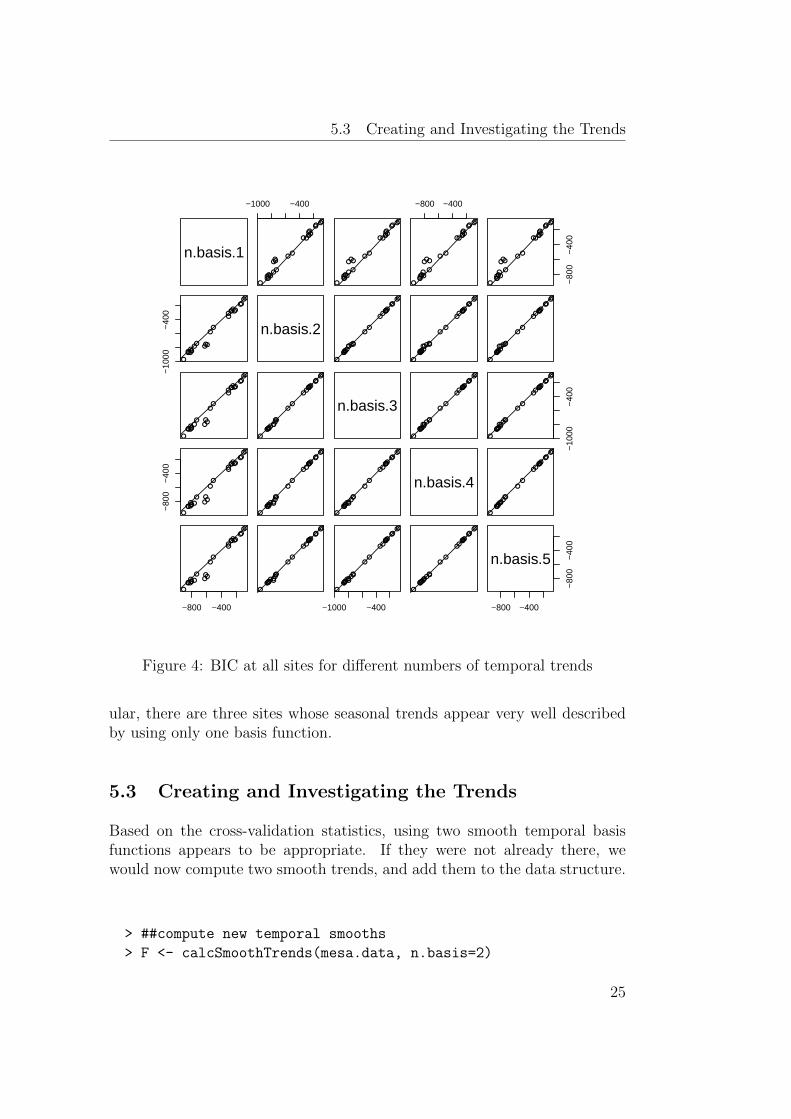
5.3 Creating and Investigating the Trends
n.basis.1
−1000 −400
●●
●●
●●●●●
●
●
●
●●
●●●
●●
●
●●
●●
●
●●
●●
●●●●●
●
●
●
●●
●●●
●●
●
●●
●●
●
−800 −400
●●
●●
●●●●●
●
●
●
●●
●●●
●●
●
●●
●●
●
−80
0−
400
●●
●●
●●●●●
●
●
●
●●
●●●
●●
●
●●
●●
●
−10
00−
400
●●
●●
●
●●●●
●
●
●
●●
●●●
●
●
●
●●
●●
●
n.basis.2●●
●●
●
●●●●
●
●
●
●●
●●●
●
●
●
●●
●●
●
●●
●●
●
●●●●
●
●
●
●●
●●●
●
●
●
●●
●●
●
●●
●●
●
●●●●
●
●
●
●●
●●●
●
●
●
●●
●●
●
●●
●●
●
●●●●
●
●
●
●●
●●●
●
●
●
●●
●●
●
●●
●●
●
●●●●
●
●
●
●●
●●●
●
●
●
●●
●●
●
n.basis.3●●
●●
●
●●●●
●
●
●
●●
●●●
●
●
●
●●
●●
●
−10
00−
400
●●
●●
●
●●●●
●
●
●
●●
●●●
●
●
●
●●
●●
●
−80
0−
400
●●
●●
●
●●●●
●
●
●
●●
●●●
●
●
●
●●
●●
●
●●
●●
●
●●●●
●
●
●
●●
●●●
●
●
●
●●
●●
●
●●
●●
●
●●●●
●
●
●
●●
●●●
●
●
●
●●
●●
●
n.basis.4●●
●●
●
●●●●
●
●
●
●●
●●●
●
●
●
●●
●●
●
−800 −400
●●
●●
●
●●●●
●
●
●
●●
●●●
●
●
●
●●
●●
●
●●
●●
●
●●●●
●
●
●
● ●
●●●
●
●
●
●●
●●
●
−1000 −400
●●
●●
●
●●●●
●
●
●
●●
●●●
●
●
●
●●
●●
●
●●
●●
●
●●●●
●
●
●
●●
●●●
●
●
●
●●
●●
●
−800 −400
−80
0−
400
n.basis.5
Figure 4: BIC at all sites for different numbers of temporal trends
ular, there are three sites whose seasonal trends appear very well describedby using only one basis function.
5.3 Creating and Investigating the Trends
Based on the cross-validation statistics, using two smooth temporal basisfunctions appears to be appropriate. If they were not already there, wewould now compute two smooth trends, and add them to the data structure.
> ##compute new temporal smooths
> F <- calcSmoothTrends(mesa.data, n.basis=2)
25

Tutorial for SpatioTemporal
> ##and add the new trends to the data structure
> mesa.data$trend <- F$trend
Alternatively (and more efficiently), if mesa.data did not contain any tem-poral trends, we could use the updateSTdataTrend() function to add themto the data structure:
> ##compute new temporal smooths
> mesa.data <- updateSTdataTrend(mesa.data, n.basis=2)
Given smooth trends we fit the time series of observations to the trends ateach site, and study the residuals (see Figure 5).
> ##plot the observations at two of the locations along
> ##with the fitted smooth trends, see Figure 5
> par(mfrow=c(4,1),mar=c(2.5,2.5,2,.5))
> plot(mesa.data, "obs", ID=5)
> plot(mesa.data, "obs", ID=18)
> ##also plot the residuals
> plot(mesa.data, "res", ID=5)
> plot(mesa.data, "res", ID=18)
The function plot.STdata fits a linear regression of observations for a par-ticular site on the smooth basis functions, and plots either fitted values,residuals or the auto-correlation function. From Figure 5 we can see thatthe fitted seasonal variability is different for the two sites (with greater sea-sonal variability in log NOx for Site 60590007), and furthermore that forSite 60590007, the fit extends earlier in time than observations are made.Both of the fits elicit residuals that are centred around 0, indicating that thetemporal trends do a good job of describing the temporal variability of theobserved log NOx concentrations.
Since we want the temporal trends to capture the temporal variability wealso study the auto correlation function of the residuals to determine howmuch temporal dependence remains after fitting the temporal trends. Ifthe temporal trends do a good job of capturing temporal variability, thereshould be little to no temporal correlation in the residuals. To investigatehow well the trends have captured the temporal variability we study theauto-correlation plots in Figure 6.
26
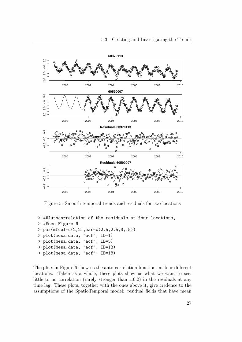
5.3 Creating and Investigating the Trends
●
●●
●
●●
●
●
●●●●
●●
●
●●●●
●●●●●●●●
●●●●
●●●●●
●●
●
●●
●●
●●
●
●●●
●
●
●
●●●●
●●
●
●●
●●
●●
●●●
●
●
●●●●
●
●
●●●
●
●●
●●
●●●●●●
●●●
●●
●●●
●
●●●
●
●●●●
●●
●●●
●●
●
●●
●
●
●●●●●
●
●●●●●●●●
●
●
●●●●
●
●
●
●
●
●●●
●●
●●●●●●●
●
●
●●●●
●●
●●●
●
●
●
●
●●
●●
●●●
●●●●
●●●●●
●
●●
●●
●●●●●
●●
●●
●●
●●●
●●●●●●
●●
●
●●●
●
●●●●
●
●●●●
●
●
●●
●●
●
●
●
●●●
●
●
●●●●
●●●●
●●
●●
●
●
●
●●●●●
●
●
●●
●●●
●●●●
●●●
●
●
●
2000 2002 2004 2006 2008 2010
2.0
3.0
4.0
5.0
60370113
date
●
●●
●●
●
●
●●●
●●
●
●●
●●
●●●●
●●●●●
●●●
●
●
●
●
●
●
●●
●
●●
●●
●
●●●
●
●●●
●●●●
●
●●●●●●●
●●●
●
●●
●
●
●
●●●
●●●
●
●●
●●
●●●
●
●
●
●
●
●●●●●
●●
●●
●●●●●
●●
●●●●
●●●
●●●●●
●●●
●●●●●●●
●
●
●●
●●●●●●●●
●●●●
●●●
●●●●●
●●●●●
●
●
●●●
●
●
●
●
●●
●●●
●●
●
●
●●●●●
●
●●
●●
●
●●●
●
●
●
●
●●
●●
●●●●
●●●●
●
●
●
2000 2002 2004 2006 2008 2010
2.0
3.0
4.0
5.0
60590007
date
●
●●
●
●
●
●
●
●
●
●
●
●
●
●
●●●
●
●●
●●
●
●
●
●
●●●
●●●●●●
●●
●
●●
●
●
●●
●
●
●
●
●
●
●
●●●
●●
●
●
●
●
●●
●
●
●●●
●
●
●●●
●
●
●
●
●●
●
●●
●●
●
●●●
●●
●●●
●
●
●●●
●
●
●
●
●
●
●
●
●
●
●
●
●●
●●
●
●●
●
●
●
●
●
●●
●
●
●●●
●
●●●
●
●
●
●●
●
●
●
●
●
●
●
●
●
●
●
●
●●
●●●●
●
●
●
●
●●●
●
●
●●
●
●
●
●
●
●
●
●
●
●
●
●●●●●
●
●●
●
●
●
●
●
●
●●●
●
●
●●
●
●
●
●
●●●
●●●
●
●●
●
●
●
●
●●
●
●
●●
●
●
●
●●
●
●
●
●●
●
●
●
●
●
●
●●
●
●
●
●●
●
●
●●●●●
●●
●
●
●
●●●
●●
●
●
●
●
●
●●
●●●●
●●
●
●
●
●
2000 2002 2004 2006 2008 2010
−0.
50.
00.
5
Residuals 60370113
date
●
●
●
●
●
●
●
●●
●
●
●
●●
●
●
●
●●●
●
●●
●
●
●
●
●
●
●
●
●
●
●
●
●
●
●
●
●●
●
●
●
●●
●
●
●●
●
●
●●
●
●●
●●●●
●
●
●
●●
●
●
●
●
●
●
●●
●●●
●
●
●
●
●
●●●
●
●
●
●
●
●●
●
●
●
●●
●
●
●
●
●●
●
●
●
●
●
●
●
●
●●
●
●●●●
●
●●
●
●
●●
●●
●
●
●●
●
●●
●
●●
●●
●●●
●●
●
●●
●
●●●
●
●
●●●
●
●
●
●
●●
●
●
●
●
●
●●●
●
●
●
●
●
●●●●
●
●
●
●
●
●
●
●●●
●
●
●
●
●
●●
●
●●●
●
●●
●
●
●
●
●
2000 2002 2004 2006 2008 2010
−0.
8−
0.2
0.4
Residuals 60590007
Figure 5: Smooth temporal trends and residuals for two locations
> ##Autocorrelation of the residuals at four locations,
> ##see Figure 6
> par(mfcol=c(2,2),mar=c(2.5,2.5,3,.5))
> plot(mesa.data, "acf", ID=1)
> plot(mesa.data, "acf", ID=5)
> plot(mesa.data, "acf", ID=13)
> plot(mesa.data, "acf", ID=18)
The plots in Figure 6 show us the auto-correlation functions at four differentlocations. Taken as a whole, these plots show us what we want to see:little to no correlation (rarely stronger than ±0.2) in the residuals at anytime lag. These plots, together with the ones above it, give credence to theassumptions of the SpatioTemporal model: residual fields that have mean
27
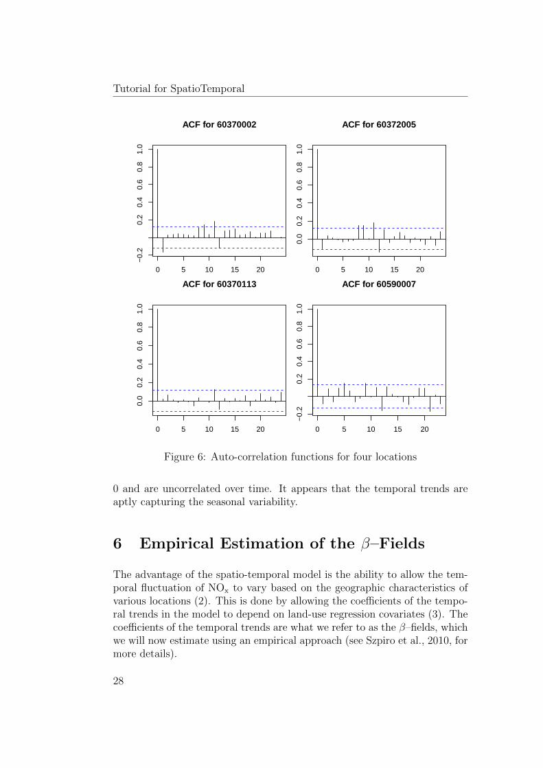
Tutorial for SpatioTemporal
0 5 10 15 20
−0.
20.
20.
40.
60.
81.
0
Lag
ACF for 60370002
0 5 10 15 20
0.0
0.2
0.4
0.6
0.8
1.0
ACF for 60370113
0 5 10 15 20
0.0
0.2
0.4
0.6
0.8
1.0
LagA
CF
ACF for 60372005
0 5 10 15 20
−0.
20.
20.
40.
60.
81.
0
AC
FACF for 60590007
Figure 6: Auto-correlation functions for four locations
0 and are uncorrelated over time. It appears that the temporal trends areaptly capturing the seasonal variability.
6 Empirical Estimation of the β–Fields
The advantage of the spatio-temporal model is the ability to allow the tem-poral fluctuation of NOx to vary based on the geographic characteristics ofvarious locations (2). This is done by allowing the coefficients of the tempo-ral trends in the model to depend on land-use regression covariates (3). Thecoefficients of the temporal trends are what we refer to as the β–fields, whichwe will now estimate using an empirical approach (see Szpiro et al., 2010, formore details).
28
6. Empirical Estimation of the β–Fields
Recall D, which was the 280×25 data matrix of the n = 25 locations with the(up to) T = 280 observations over time. Given smooth temporal trends wefit each of the times series of observations to the smooth trends and extractthe regression coefficients.
> ##create data matrix
> D <- createDataMatrix(mesa.data)
> beta <- matrix(NA,dim(D)[2], dim(mesa.data$trend)[2])
> beta.std <- beta
> ##extact the temporal trends
> F <- mesa.data$trend
> ##drop the date column
> F$date <- NULL
> ##estimate the beta-coeficients at each location
> for(i in 1:dim(D)[2]){
tmp <- lm(D[,i] ~ as.matrix(F))
beta[i,] <- coef(tmp)
beta.std[i,] <- sqrt(diag(vcov(tmp)))
}
> ##Add names to the estimated betas
> colnames(beta) <- c("const",colnames(F))
> rownames(beta) <- colnames(D)
> dimnames(beta.std) <- dimnames(beta)
Finally we study the estimated regression coefficients:
> ##examine the beta fields
> head(beta)
const V1 V2
60370002 3.698932 -0.20189383 0.25751993
60370016 3.372849 -0.07064596 0.24127792
60370030 4.206123 -0.48859878 0.15939586
60370031 3.719557 -0.64148029 -0.04067102
60370113 3.527936 -0.51028700 0.07050822
60371002 4.173345 -0.46945537 0.12826088
And the uncertainty in the estimation
> head(beta.std)
29

Tutorial for SpatioTemporal
const V1 V2
60370002 0.01447987 0.01447860 0.01456190
60370016 0.01332344 0.01335100 0.01335100
60370030 0.04656093 0.03761209 0.04388509
60370031 0.07273316 0.04202223 0.06416097
60370113 0.01547441 0.01547949 0.01547938
60371002 0.01278047 0.01278508 0.01279324
These are the β–fields that will be modelled using geographic covariates in thefull spatio-temporal model. Here, beta is a 25 × 3 matrix with β0(s), β1(s),and β2(s) representing regression coefficients for the intercept and two tem-poral trends at each of the 25 locations.
The selection of geographic covariates could be done by comparing these fieldsto the available covariates. However, the variable selection is outside thescope of this tutorial (see Mercer et al., 2011, for some possible alternatives).For now we just keep the values and will (eventually) compare them to resultsfrom the full model.
7 createSTmodel(): Specifying the Spatio-Temporal
model
This section discusses how to specify everything we need to fit the Spatio-Temporal model. Recall that the covariance matrices of each βi-field is char-acterised by two parameters, φi and σ2
i , where φi is the range and σ2i is the
partial sill (5); we are assuming a zero nugget for the β-fields. The covariancefor the spatio-temporal residuals are characterised by three parameters, φν ,σ2ν , and τ 2ν (6); respectively denoting range, partial sill and nugget (Lind-
strom et al., 2011, Sampson et al., 2009, Szpiro et al., 2010). These are theparameters that we need to estimate using maximum-likelihood. We needto specify the type of spatial covariance model (e.g., exponential) to use foreach β-fields and the ν-field, and define the covariates we want for each ofthe β-fields. The regression parameters (4) are implicitly estimated since wewill be using a profile likelihood formulation, see Lindstrom et al. (2011) fordetails.
First we will create the input for createSTmodel() that gives the LUR co-variates to be used for each of the β-fields; and define the spatial covariacemodel for each β-field and the ν-field. This is done accordingly:
30
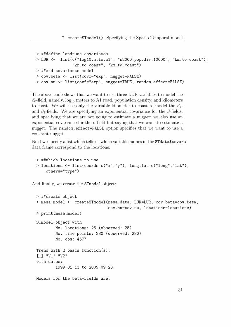
7. createSTmodel(): Specifying the Spatio-Temporal model
> ##define land-use covariates
> LUR <- list(c("log10.m.to.a1", "s2000.pop.div.10000", "km.to.coast"),
"km.to.coast", "km.to.coast")
> ##and covariance model
> cov.beta <- list(covf="exp", nugget=FALSE)
> cov.nu <- list(covf="exp", nugget=TRUE, random.effect=FALSE)
The above code shows that we want to use three LUR variables to model theβ0-field, namely, log10 meters to A1 road, population density, and kilometersto coast. We will use only the variable kilometer to coast to model the β1-and β2-fields. We are specifying an exponential covariance for the β-fields,and specifying that we are not going to estimate a nugget; we also use anexponential covariance for the ν-field but saying that we want to estimate anugget. The random.effect=FALSE option specifies that we want to use aconstant nugget.
Next we specify a list which tells us which variable names in the STdata$covarsdata frame correspond to the locations:
> ##which locations to use
> locations <- list(coords=c("x","y"), long.lat=c("long","lat"),
others="type")
And finally, we create the STmodel object:
> ##create object
> mesa.model <- createSTmodel(mesa.data, LUR=LUR, cov.beta=cov.beta,
cov.nu=cov.nu, locations=locations)
> print(mesa.model)
STmodel-object with:
No. locations: 25 (observed: 25)
No. time points: 280 (observed: 280)
No. obs: 4577
Trend with 2 basis function(s):
[1] "V1" "V2"
with dates:
1999-01-13 to 2009-09-23
Models for the beta-fields are:
31
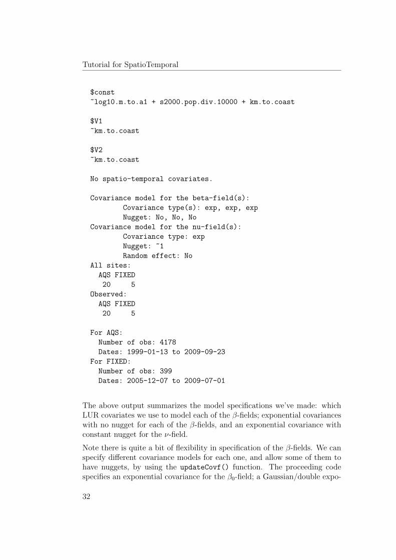
Tutorial for SpatioTemporal
$const
~log10.m.to.a1 + s2000.pop.div.10000 + km.to.coast
$V1
~km.to.coast
$V2
~km.to.coast
No spatio-temporal covariates.
Covariance model for the beta-field(s):
Covariance type(s): exp, exp, exp
Nugget: No, No, No
Covariance model for the nu-field(s):
Covariance type: exp
Nugget: ~1
Random effect: No
All sites:
AQS FIXED
20 5
Observed:
AQS FIXED
20 5
For AQS:
Number of obs: 4178
Dates: 1999-01-13 to 2009-09-23
For FIXED:
Number of obs: 399
Dates: 2005-12-07 to 2009-07-01
The above output summarizes the model specifications we’ve made: whichLUR covariates we use to model each of the β-fields; exponential covarianceswith no nugget for each of the β-fields, and an exponential covariance withconstant nugget for the ν-field.
Note there is quite a bit of flexibility in specification of the β-fields. We canspecify different covariance models for each one, and allow some of them tohave nuggets, by using the updateCovf() function. The proceeding codespecifies an exponential covariance for the β0-field; a Gaussian/double expo-
32
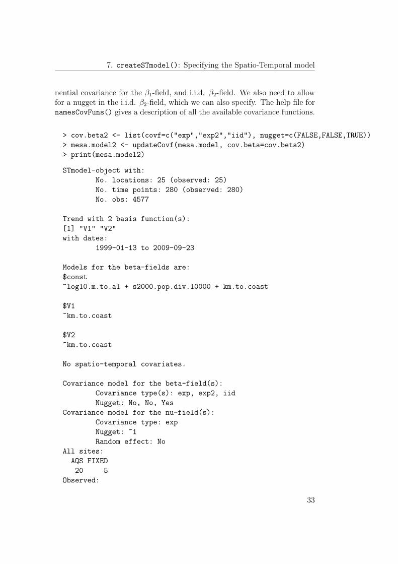
7. createSTmodel(): Specifying the Spatio-Temporal model
nential covariance for the β1-field, and i.i.d. β2-field. We also need to allowfor a nugget in the i.i.d. β2-field, which we can also specify. The help file fornamesCovFuns() gives a description of all the available covariance functions.
> cov.beta2 <- list(covf=c("exp","exp2","iid"), nugget=c(FALSE,FALSE,TRUE))
> mesa.model2 <- updateCovf(mesa.model, cov.beta=cov.beta2)
> print(mesa.model2)
STmodel-object with:
No. locations: 25 (observed: 25)
No. time points: 280 (observed: 280)
No. obs: 4577
Trend with 2 basis function(s):
[1] "V1" "V2"
with dates:
1999-01-13 to 2009-09-23
Models for the beta-fields are:
$const
~log10.m.to.a1 + s2000.pop.div.10000 + km.to.coast
$V1
~km.to.coast
$V2
~km.to.coast
No spatio-temporal covariates.
Covariance model for the beta-field(s):
Covariance type(s): exp, exp2, iid
Nugget: No, No, Yes
Covariance model for the nu-field(s):
Covariance type: exp
Nugget: ~1
Random effect: No
All sites:
AQS FIXED
20 5
Observed:
33
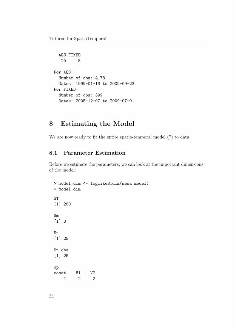
Tutorial for SpatioTemporal
AQS FIXED
20 5
For AQS:
Number of obs: 4178
Dates: 1999-01-13 to 2009-09-23
For FIXED:
Number of obs: 399
Dates: 2005-12-07 to 2009-07-01
8 Estimating the Model
We are now ready to fit the entire spatio-temporal model (7) to data.
8.1 Parameter Estimation
Before we estimate the parameters, we can look at the important dimensionsof the model:
> model.dim <- loglikeSTdim(mesa.model)
> model.dim
$T
[1] 280
$m
[1] 3
$n
[1] 25
$n.obs
[1] 25
$p
const V1 V2
4 2 2
34
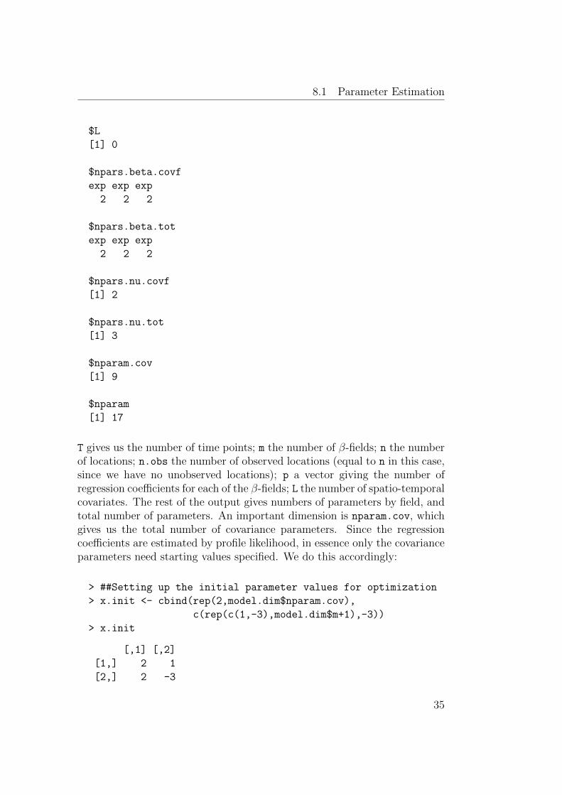
8.1 Parameter Estimation
$L
[1] 0
$npars.beta.covf
exp exp exp
2 2 2
$npars.beta.tot
exp exp exp
2 2 2
$npars.nu.covf
[1] 2
$npars.nu.tot
[1] 3
$nparam.cov
[1] 9
$nparam
[1] 17
T gives us the number of time points; m the number of β-fields; n the numberof locations; n.obs the number of observed locations (equal to n in this case,since we have no unobserved locations); p a vector giving the number ofregression coefficients for each of the β-fields; L the number of spatio-temporalcovariates. The rest of the output gives numbers of parameters by field, andtotal number of parameters. An important dimension is nparam.cov, whichgives us the total number of covariance parameters. Since the regressioncoefficients are estimated by profile likelihood, in essence only the covarianceparameters need starting values specified. We do this accordingly:
> ##Setting up the initial parameter values for optimization
> x.init <- cbind(rep(2,model.dim$nparam.cov),
c(rep(c(1,-3),model.dim$m+1),-3))
> x.init
[,1] [,2]
[1,] 2 1
[2,] 2 -3
35

Tutorial for SpatioTemporal
[3,] 2 1
[4,] 2 -3
[5,] 2 1
[6,] 2 -3
[7,] 2 1
[8,] 2 -3
[9,] 2 -3
Here each column of x.init contains a starting value for the optimisa-tion process in estimating the MLE’s of the 9 covariance parameters. Notethat these are starting values for only the optimisation of the covarianceparameters; once those have been optimised, the maximum-likelihood es-timate of the regression coefficients can be inferred using generalised leastsquares (see Lindstrom et al., 2011, for details). In general x.init shouldbe a (nparam.cov)-by-(number of starting points) matrix, or just a vector oflength nparam.cov vector if only one starting point is desired.
What parameters are we specifying the starting points for? We can verifythis using loglikeSTnames:
> loglikeSTnames(mesa.model,all=FALSE)
[1] "log.range.const.exp"
[2] "log.sill.const.exp"
[3] "log.range.V1.exp"
[4] "log.sill.V1.exp"
[5] "log.range.V2.exp"
[6] "log.sill.V2.exp"
[7] "nu.log.range.exp"
[8] "nu.log.sill.exp"
[9] "nu.log.nugget.(Intercept).exp"
This gives the order of variables in x.init and also tells us which of theparameters are logged. Specifying all=FALSE gives us only the covarianceparameters.
> ##Add names to the initial values
> rownames(x.init) <- loglikeSTnames(mesa.model,all=FALSE)
> x.init
[,1] [,2]
log.range.const.exp 2 1
36
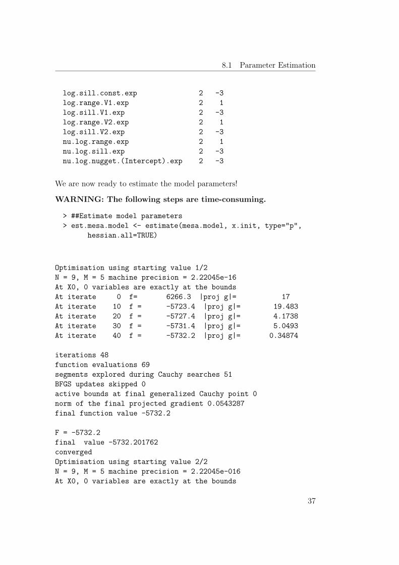
8.1 Parameter Estimation
log.sill.const.exp 2 -3
log.range.V1.exp 2 1
log.sill.V1.exp 2 -3
log.range.V2.exp 2 1
log.sill.V2.exp 2 -3
nu.log.range.exp 2 1
nu.log.sill.exp 2 -3
nu.log.nugget.(Intercept).exp 2 -3
We are now ready to estimate the model parameters!
WARNING: The following steps are time-consuming.
> ##Estimate model parameters
> est.mesa.model <- estimate(mesa.model, x.init, type="p",
hessian.all=TRUE)
Optimisation using starting value 1/2
N = 9, M = 5 machine precision = 2.22045e-16
At X0, 0 variables are exactly at the bounds
At iterate 0 f= 6266.3 |proj g|= 17
At iterate 10 f = -5723.4 |proj g|= 19.483
At iterate 20 f = -5727.4 |proj g|= 4.1738
At iterate 30 f = -5731.4 |proj g|= 5.0493
At iterate 40 f = -5732.2 |proj g|= 0.34874
iterations 48
function evaluations 69
segments explored during Cauchy searches 51
BFGS updates skipped 0
active bounds at final generalized Cauchy point 0
norm of the final projected gradient 0.0543287
final function value -5732.2
F = -5732.2
final value -5732.201762
converged
Optimisation using starting value 2/2
N = 9, M = 5 machine precision = 2.22045e-016
At X0, 0 variables are exactly at the bounds
37
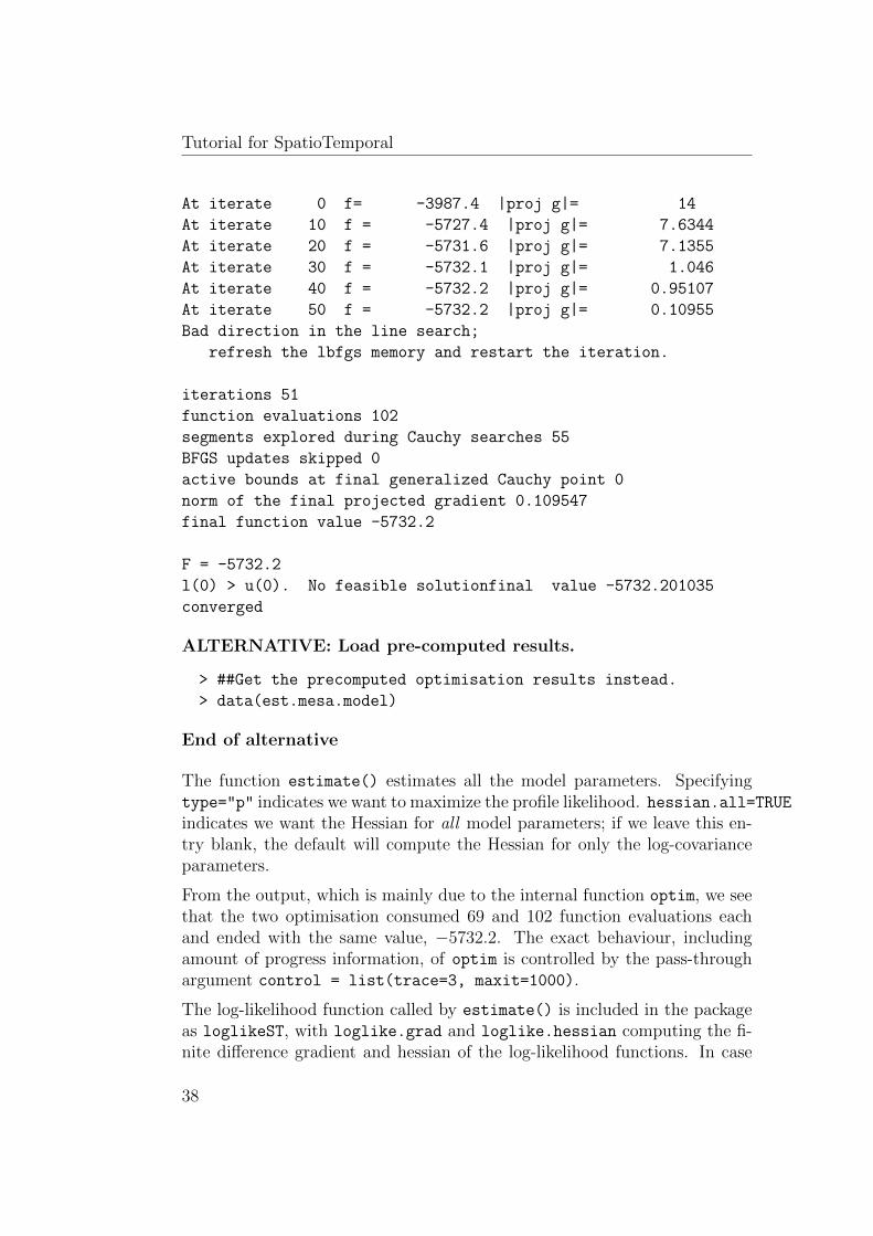
Tutorial for SpatioTemporal
At iterate 0 f= -3987.4 |proj g|= 14
At iterate 10 f = -5727.4 |proj g|= 7.6344
At iterate 20 f = -5731.6 |proj g|= 7.1355
At iterate 30 f = -5732.1 |proj g|= 1.046
At iterate 40 f = -5732.2 |proj g|= 0.95107
At iterate 50 f = -5732.2 |proj g|= 0.10955
Bad direction in the line search;
refresh the lbfgs memory and restart the iteration.
iterations 51
function evaluations 102
segments explored during Cauchy searches 55
BFGS updates skipped 0
active bounds at final generalized Cauchy point 0
norm of the final projected gradient 0.109547
final function value -5732.2
F = -5732.2
l(0) > u(0). No feasible solutionfinal value -5732.201035
converged
ALTERNATIVE: Load pre-computed results.
> ##Get the precomputed optimisation results instead.
> data(est.mesa.model)
End of alternative
The function estimate() estimates all the model parameters. Specifyingtype="p" indicates we want to maximize the profile likelihood. hessian.all=TRUEindicates we want the Hessian for all model parameters; if we leave this en-try blank, the default will compute the Hessian for only the log-covarianceparameters.
From the output, which is mainly due to the internal function optim, we seethat the two optimisation consumed 69 and 102 function evaluations eachand ended with the same value, −5732.2. The exact behaviour, includingamount of progress information, of optim is controlled by the pass-throughargument control = list(trace=3, maxit=1000).
The log-likelihood function called by estimate() is included in the packageas loglikeST, with loglike.grad and loglike.hessian computing the fi-nite difference gradient and hessian of the log-likelihood functions. In case
38
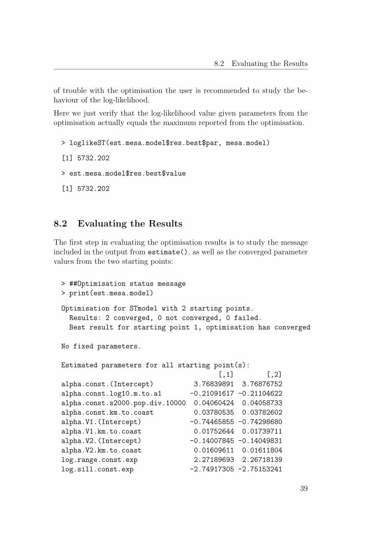
8.2 Evaluating the Results
of trouble with the optimisation the user is recommended to study the be-haviour of the log-likelihood.
Here we just verify that the log-likelihood value given parameters from theoptimisation actually equals the maximum reported from the optimisation.
> loglikeST(est.mesa.model$res.best$par, mesa.model)
[1] 5732.202
> est.mesa.model$res.best$value
[1] 5732.202
8.2 Evaluating the Results
The first step in evaluating the optimisation results is to study the messageincluded in the output from estimate(), as well as the converged parametervalues from the two starting points:
> ##Optimisation status message
> print(est.mesa.model)
Optimisation for STmodel with 2 starting points.
Results: 2 converged, 0 not converged, 0 failed.
Best result for starting point 1, optimisation has converged
No fixed parameters.
Estimated parameters for all starting point(s):
[,1] [,2]
alpha.const.(Intercept) 3.76839891 3.76876752
alpha.const.log10.m.to.a1 -0.21091617 -0.21104622
alpha.const.s2000.pop.div.10000 0.04060424 0.04058733
alpha.const.km.to.coast 0.03780535 0.03782602
alpha.V1.(Intercept) -0.74465855 -0.74298680
alpha.V1.km.to.coast 0.01752644 0.01739711
alpha.V2.(Intercept) -0.14007845 -0.14049831
alpha.V2.km.to.coast 0.01609611 0.01611804
log.range.const.exp 2.27189693 2.26718139
log.sill.const.exp -2.74917305 -2.75153241
39
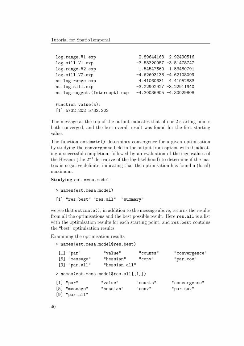
Tutorial for SpatioTemporal
log.range.V1.exp 2.89644168 2.92490516
log.sill.V1.exp -3.53320957 -3.51478747
log.range.V2.exp 1.54547660 1.53480791
log.sill.V2.exp -4.62603138 -4.62108099
nu.log.range.exp 4.41060631 4.41052883
nu.log.sill.exp -3.22902927 -3.22911940
nu.log.nugget.(Intercept).exp -4.30036905 -4.30029808
Function value(s):
[1] 5732.202 5732.202
The message at the top of the output indicates that of our 2 starting pointsboth converged, and the best overall result was found for the first startingvalue.
The function estimate() determines convergence for a given optimisationby studying the convergence field in the output from optim, with 0 indicat-ing a successful completion; followed by an evaluation of the eigenvalues ofthe Hessian (the 2nd derivative of the log-likelihood) to determine if the ma-trix is negative definite; indicating that the optimisation has found a (local)maximum.
Studying est.mesa.model:
> names(est.mesa.model)
[1] "res.best" "res.all" "summary"
we see that estimate(), in addition to the message above, returns the resultsfrom all the optimisations and the best possible result. Here res.all is a listwith the optimisation results for each starting point, and res.best containsthe “best” optimisation results.
Examining the optimisation results
> names(est.mesa.model$res.best)
[1] "par" "value" "counts" "convergence"
[5] "message" "hessian" "conv" "par.cov"
[9] "par.all" "hessian.all"
> names(est.mesa.model$res.all[[1]])
[1] "par" "value" "counts" "convergence"
[5] "message" "hessian" "conv" "par.cov"
[9] "par.all"
40
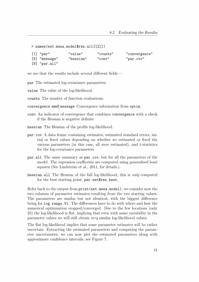
8.2 Evaluating the Results
> names(est.mesa.model$res.all[[2]])
[1] "par" "value" "counts" "convergence"
[5] "message" "hessian" "conv" "par.cov"
[9] "par.all"
we see that the results include several different fields —
par The estimated log-covariance parameters.
value The value of the log-likelihood.
counts The number of function evaluations.
convergence and message Convergence information from optim.
conv An indicator of convergence that combines convergence with a checkif the Hessian is negative definite
hessian The Hessian of the profile log-likelihood.
par.cov A data frame containing estimates, estimated standard errors, ini-tial or fixed values depending on whether we estimated or fixed thevarious parameters (in this case, all were estimated), and t-statisticsfor the log-covariance parameters
par.all The same summary as par.cov, but for all the parameters of themodel. The regression coefficents are computed using generalised leastsquares (See Lindstrom et al., 2011, for details.).
hessian.all The Hessian of the full log-likelihood, this is only computedfor the best starting point, par.est$res.best.
Refer back to the output from print(est.mesa.model); we consider now thetwo columns of parameter estimates resulting from the two starting values.The parameters are similar but not identical, with the biggest differencebeing for log.range.V1. The differences have to do with where and how thenumerical optimisation stopped/converged. Due to the few locations (only25) the log-likelihood is flat, implying that even with some variability in theparameter values we will still obtain very similar log-likelihood values.
The flat log-likelihood implies that some parameter estimates will be ratheruncertain. Extracting the estimated parameters and computing the param-eter uncertainties, we can now plot the estimated parameters along withapproximate confidence intervals, see Figure 7.
41

Tutorial for SpatioTemporal
> ##extract the estimated parameters and approximate uncertainties
> x <- est.mesa.model$res.best$par.all
##Plot the estimated parameters with uncertainties, see Figure 7
> ##plot the estimated parameters with uncertainties
> par(mfrow=c(1,1),mar=c(13.5,2.5,.5,.5))
> plot(x$par, ylim=range(c( x$par-1.96*x$sd, x$par+1.96*x$sd )),
xlab="", xaxt="n")
> points(x$par - 1.96*x$sd, pch=3)
> points(x$par + 1.96*x$sd, pch=3)
> axis(1, 1:length(x$par), rownames(x), las=2)
●
●● ●
●
● ● ●
●
●
●
●
●
●
●
●
●−4
−2
02
4
alph
a.co
nst.(
Inte
rcep
t)
alph
a.co
nst.l
og10
.m.to
.a1
alph
a.co
nst.s
2000
.pop
.div
.100
00
alph
a.co
nst.k
m.to
.coa
st
alph
a.V
1.(I
nter
cept
)
alph
a.V
1.km
.to.c
oast
alph
a.V
2.(I
nter
cept
)
alph
a.V
2.km
.to.c
oast
log.
rang
e.co
nst.e
xp
log.
sill.
cons
t.exp
log.
rang
e.V
1.ex
p
log.
sill.
V1.
exp
log.
rang
e.V
2.ex
p
log.
sill.
V2.
exp
nu.lo
g.ra
nge.
exp
nu.lo
g.si
ll.ex
p
nu.lo
g.nu
gget
.(In
terc
ept)
.exp
Figure 7: Estimated parameters and their 95% confidence intervals from thefirst starting point.
42
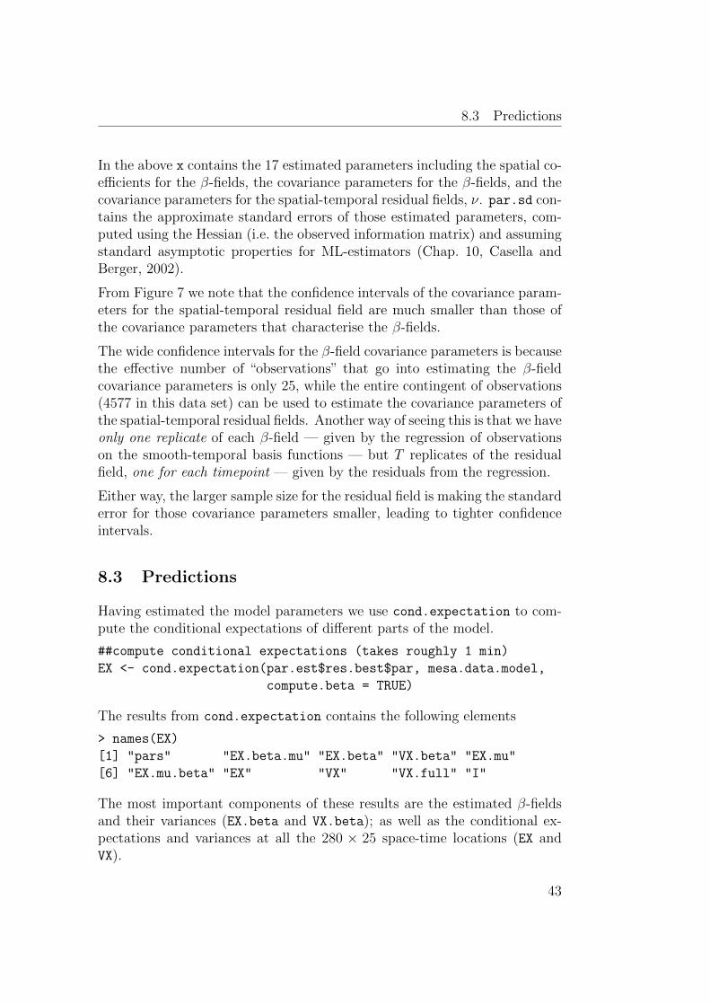
8.3 Predictions
In the above x contains the 17 estimated parameters including the spatial co-efficients for the β-fields, the covariance parameters for the β-fields, and thecovariance parameters for the spatial-temporal residual fields, ν. par.sd con-tains the approximate standard errors of those estimated parameters, com-puted using the Hessian (i.e. the observed information matrix) and assumingstandard asymptotic properties for ML-estimators (Chap. 10, Casella andBerger, 2002).
From Figure 7 we note that the confidence intervals of the covariance param-eters for the spatial-temporal residual field are much smaller than those ofthe covariance parameters that characterise the β-fields.
The wide confidence intervals for the β-field covariance parameters is becausethe effective number of “observations” that go into estimating the β-fieldcovariance parameters is only 25, while the entire contingent of observations(4577 in this data set) can be used to estimate the covariance parameters ofthe spatial-temporal residual fields. Another way of seeing this is that we haveonly one replicate of each β-field — given by the regression of observationson the smooth-temporal basis functions — but T replicates of the residualfield, one for each timepoint — given by the residuals from the regression.
Either way, the larger sample size for the residual field is making the standarderror for those covariance parameters smaller, leading to tighter confidenceintervals.
8.3 Predictions
Having estimated the model parameters we use cond.expectation to com-pute the conditional expectations of different parts of the model.
##compute conditional expectations (takes roughly 1 min)
EX <- cond.expectation(par.est$res.best$par, mesa.data.model,
compute.beta = TRUE)
The results from cond.expectation contains the following elements
> names(EX)
[1] "pars" "EX.beta.mu" "EX.beta" "VX.beta" "EX.mu"
[6] "EX.mu.beta" "EX" "VX" "VX.full" "I"
The most important components of these results are the estimated β-fieldsand their variances (EX.beta and VX.beta); as well as the conditional ex-pectations and variances at all the 280 × 25 space-time locations (EX andVX).
43

Tutorial for SpatioTemporal
All the components of EX are compute conditional on the estimated param-eters and observed data; the components are:
pars The regression parameters in (4), computed using generalised leastsquares (see Lindstrom et al., 2011, for details).
EX.beta The expected latent β-fields.
EX.beta.mu The mean component of the latent β-fields, i.e. the Xiαi partof (3).
VX.beta The conditional variance of the latent β-fields in EX.beta.
EX The expected spatio-temporal process (1), orE(y(s, t)|Ψ, observations).
EX.mu The regression component of the spatio-temporal process,
µ(s, t) =L∑l=1
γlMl(s, t) +m∑i=1
Xiαifi(t).
Note that this differs from (2).
EX.mu.beta The mean part (2) of the spatio-temporal process (1).
VX The conditional variance of the spatio-temporal process in EX.
VX.full A list containing the temporal covariance matrix for each recon-structed time-series. This is needed to correctly compute confidenceintervalls for long term average pollution at each location.
I An index vector that can be used to extract the observed spatio-temporallocations from EX, EX.mu, and/or EX.mu.beta.
The decomposition of the predictions could potentially be used for modelevaluation.
First we compare the β-fields computed by fitting each of the times seriesof observations to the smooth trends, with the β-fields obtained from thefull model. Recall that the simple, or empirical, estimate of the β-fields wascomputed in Section 6 above with the results are contained in the beta.
##Plot that compares two estimated beta-fields, see Figure 8
44

8.3 Predictions
par(mfcol=c(1,1), mar=c(4.5,4.5,2,.5), pty="s")
plotCI(x=beta[,1], y=EX$EX.beta[,1],
uiw=1.96*beta.std[,1], err="x",
main="Intercept", pch=NA, sfrac=0.005,
xlab="Empirical estimate",
ylab="Spatio-Temporal Model")
plotCI(x=beta[,1],y=EX$EX.beta[,1],
uiw=1.96*sqrt(EX$VX.beta[,1]),
add=TRUE, pch=NA, sfrac=0.005)
abline(0,1,col="grey")
The above code compares the two estimates of the β-field for f1(t) ≡ 1 andproduces Figure 8. We can of course also look at the β-fields for the twosmooth temporal trend, f2 and f3.
##Plot that compares the other beta-fields, see Figure 9par(mfcol=c(1,2), mar=c(4.5,4.5,2,.5), pty="s")
for(i in 2:3){
plotCI(x=beta[,i], y=EX$EX.beta[,i],
uiw=1.96*beta.std[,i], err="x",
main=colnames(beta)[i], pch=NA, sfrac=0.005,
xlab="Empirical estimate",
ylab="Spatio-Temporal Model")
plotCI(x=beta[,i],y=EX$EX.beta[,i],
uiw=1.96*sqrt(EX$VX.beta[,i]),
add=TRUE, pch=NA, sfrac=0.005)
abline(0,1,col="grey")
}
We can see from Figure 8 and 9 that the two ways of computing the β-fields lead to very comparable results. The largest discrepancies lie with thecoefficient for the second temporal trend, where it appears the coefficientscalculated via conditional expectation are larger than those calculated byfitting the time series to the temporal trend. However, the uncertainty inthese coefficients is large.
In addition to predictions of the β-fields, cond.expectation also computesthe conditional expectation at all the 280× 25 space-time locations.
##plot predictions and observations for 4 locations, see Figure 10par(mfrow=c(4,1),mar=c(2.5,2.5,2,.5))
plotPrediction(EX, 1, mesa.data.model)
lines(as.Date(rownames(EX$EX.mu)),EX$EX.mu[,1],col=3)
45
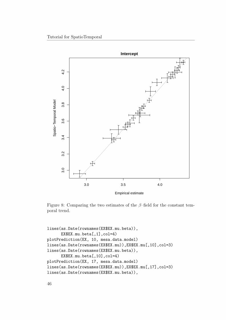
Tutorial for SpatioTemporal
3.0 3.5 4.0
3.0
3.2
3.4
3.6
3.8
4.0
4.2
Intercept
Empirical estimate
Spa
tio−
Tem
pora
l Mod
el
Figure 8: Comparing the two estimates of the β–field for the constant tem-poral trend.
lines(as.Date(rownames(EX$EX.mu.beta)),
EX$EX.mu.beta[,1],col=4)
plotPrediction(EX, 10, mesa.data.model)
lines(as.Date(rownames(EX$EX.mu)),EX$EX.mu[,10],col=3)
lines(as.Date(rownames(EX$EX.mu.beta)),
EX$EX.mu.beta[,10],col=4)
plotPrediction(EX, 17, mesa.data.model)
lines(as.Date(rownames(EX$EX.mu)),EX$EX.mu[,17],col=3)
lines(as.Date(rownames(EX$EX.mu.beta)),
46

9. Cross-validation
−1.0 −0.8 −0.6 −0.4 −0.2
−0.
8−
0.6
−0.
4−
0.2
V1
Empirical estimate
Spa
tio−
Tem
pora
l Mod
el
−0.4 −0.2 0.0 0.2−
0.2
0.0
0.1
0.2
V2
Empirical estimate
Spa
tio−
Tem
pora
l Mod
el
Figure 9: Comparing the two estimates of the β–field for the two smoothtemporal trends.
EX$EX.mu.beta[,17],col=4)
plotPrediction(EX, 22, mesa.data.model)
lines(as.Date(rownames(EX$EX.mu)),EX$EX.mu[,22],col=3)
lines(as.Date(rownames(EX$EX.mu.beta)),
EX$EX.mu.beta[,22],col=4)
Plotting these predictions along with 95% confidence intervals, the compo-nents of the predictions, and the observations at 4 different locations indicatesthat the predictions capture the seasonal variations in the data, see Figure 10.Since the predictions are conditional on the observations (and estimated pa-rameters) predictions at the observed locations of course coincides with theobservations. Adding the components of the predictions that are due to onlythe regression (green) and both regression and β-fields (blue) allows us toinvestigate how the different parts of the model capture observations.
9 Cross-validation
As a last step in the tutorial we will study a cross-validation (CV) example.The first step is to define 10 CV groups:
##create the CV structure defining 10 different CV-groups
47

Tutorial for SpatioTemporal
2000 2002 2004 2006 2008 2010
3.0
3.5
4.0
4.5
60370002
2000 2002 2004 2006 2008 2010
3.0
4.0
5.0
60371601
2000 2002 2004 2006 2008 2010
23
45
60590001
2000 2002 2004 2006 2008 2010
3.5
4.5
5.5
L002
Figure 10: The predicted and observed data for 4 of the 25 locations. Thered-lines denote observations, the black line and grey shading give predictionsand 95% confidence intervals at unobserved time-points. The green and bluegive the contribution to the predictions from the regression and regression +β-fields respectively.
> Ind.cv <- createCV(mesa.data.model, groups=10, min.dist=.1)
> head(Ind.cv)
[,1] [,2] [,3] [,4] [,5] [,6] [,7] [,8] [,9] [,10]
[1,] TRUE FALSE FALSE FALSE FALSE FALSE FALSE FALSE FALSE FALSE
[2,] FALSE FALSE TRUE FALSE FALSE FALSE FALSE FALSE FALSE FALSE
[3,] FALSE FALSE FALSE FALSE FALSE FALSE FALSE TRUE FALSE FALSE
[4,] FALSE TRUE FALSE FALSE FALSE FALSE FALSE FALSE FALSE FALSE
48

9. Cross-validation
[5,] FALSE FALSE FALSE FALSE FALSE FALSE FALSE FALSE FALSE TRUE
[6,] FALSE FALSE FALSE TRUE FALSE FALSE FALSE FALSE FALSE FALSE
Here Ind.cv is a 4577 × 10 matrix where each column defines a CV-group.The columns contain logical values indicating which of the observations toleave out. For each column, we are going to use our model to predict at theobservations marked by TRUE using all of the observations marked FALSE.Once we have done this for each CV-group/column we can compare ourpredictions to the truth and calculate cross-validated statistics such as RMSEand R2.
However first we will take a closer look at the CV-groupings.
##number of observations in each CV-group
> colSums(Ind.cv)
[1] 438 389 811 556 546 165 228 487 160 797
We see that the number of observations left out of each group is ratheruneven; the main goal of createCV is to create CV-groups such that thegroups contain roughly the same number of locations ignoring the number ofobservations at each location. If there are large differences in the number ofobservations at different locations one could use the subset option to createdifferent CV-groupings for different types of locations, possibly combiningthe resulting CV-groups by Ind.cv.final = Ind.cv1 | Ind.cv2.
If we instead look at which sites that will be excluded from which CV-group:
##Which sites belong to which groups?
> ID.cv <- lapply(apply(Ind.cv,2,list),function(x)
+ unique(mesa.data.model$obs$ID[x[[1]]]))
> ID.cv
[[1]]
[1] "60370002" "L002" "LC001"
[[2]]
[1] "60371002" "60370030" "LC003"
[[3]]
[1] "60370016" "60371301" "60374002"
[[4]]
[1] "60371201" "60372005"
49
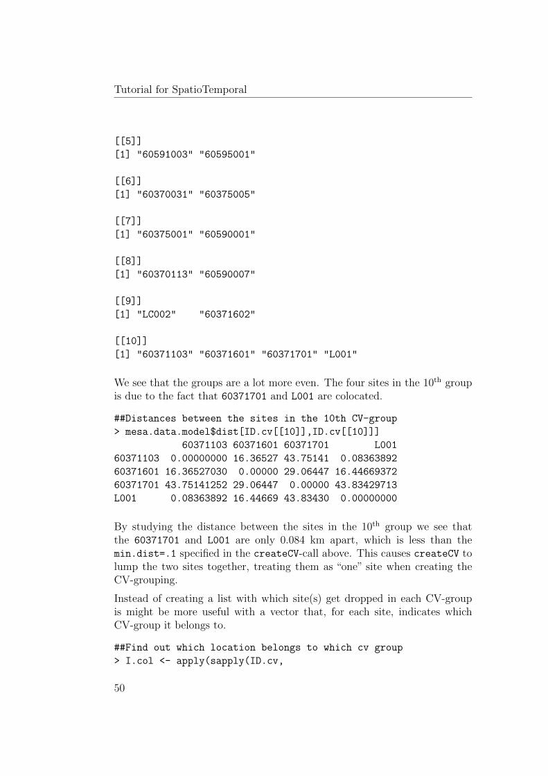
Tutorial for SpatioTemporal
[[5]]
[1] "60591003" "60595001"
[[6]]
[1] "60370031" "60375005"
[[7]]
[1] "60375001" "60590001"
[[8]]
[1] "60370113" "60590007"
[[9]]
[1] "LC002" "60371602"
[[10]]
[1] "60371103" "60371601" "60371701" "L001"
We see that the groups are a lot more even. The four sites in the 10th groupis due to the fact that 60371701 and L001 are colocated.
##Distances between the sites in the 10th CV-group
> mesa.data.model$dist[ID.cv[[10]],ID.cv[[10]]]
60371103 60371601 60371701 L001
60371103 0.00000000 16.36527 43.75141 0.08363892
60371601 16.36527030 0.00000 29.06447 16.44669372
60371701 43.75141252 29.06447 0.00000 43.83429713
L001 0.08363892 16.44669 43.83430 0.00000000
By studying the distance between the sites in the 10th group we see thatthe 60371701 and L001 are only 0.084 km apart, which is less than themin.dist=.1 specified in the createCV-call above. This causes createCV tolump the two sites together, treating them as “one” site when creating theCV-grouping.
Instead of creating a list with which site(s) get dropped in each CV-groupis might be more useful with a vector that, for each site, indicates whichCV-group it belongs to.
##Find out which location belongs to which cv group
> I.col <- apply(sapply(ID.cv,
50
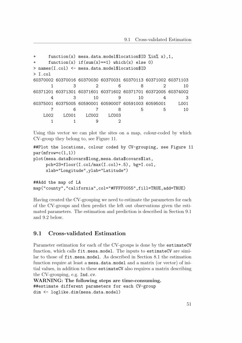
9.1 Cross-validated Estimation
+ function(x) mesa.data.model$location$ID %in% x),1,
+ function(x) if(sum(x)==1) which(x) else 0)
> names(I.col) <- mesa.data.model$location$ID
> I.col
60370002 60370016 60370030 60370031 60370113 60371002 60371103
1 3 2 6 8 2 10
60371201 60371301 60371601 60371602 60371701 60372005 60374002
4 3 10 9 10 4 3
60375001 60375005 60590001 60590007 60591003 60595001 L001
7 6 7 8 5 5 10
L002 LC001 LC002 LC003
1 1 9 2
Using this vector we can plot the sites on a map, colour-coded by whichCV-group they belong to, see Figure 11.
##Plot the locations, colour coded by CV-grouping, see Figure 11
par(mfrow=c(1,1))
plot(mesa.data$covars$long,mesa.data$covars$lat,
pch=23+floor(I.col/max(I.col)+.5), bg=I.col,
xlab="Longitude",ylab="Latitude")
##Add the map of LA
map("county","california",col="#FFFF0055",fill=TRUE,add=TRUE)
Having created the CV-grouping we need to estimate the parameters for eachof the CV-groups and then predict the left out observations given the esti-mated parameters. The estimation and prediction is described in Section 9.1and 9.2 below.
9.1 Cross-validated Estimation
Parameter estimation for each of the CV-groups is done by the estimateCV
function, which calls fit.mesa.model. The inputs to estimateCV are simi-lar to those of fit.mesa.model. As described in Section 8.1 the estimationfunction require at least a mesa.data.model and a matrix (or vector) of ini-tial values, in addition to these estimateCV also requires a matrix describingthe CV-grouping, e.g. Ind.cv.WARNING: The following steps are time-consuming.##estimate different parameters for each CV-group
dim <- loglike.dim(mesa.data.model)
51
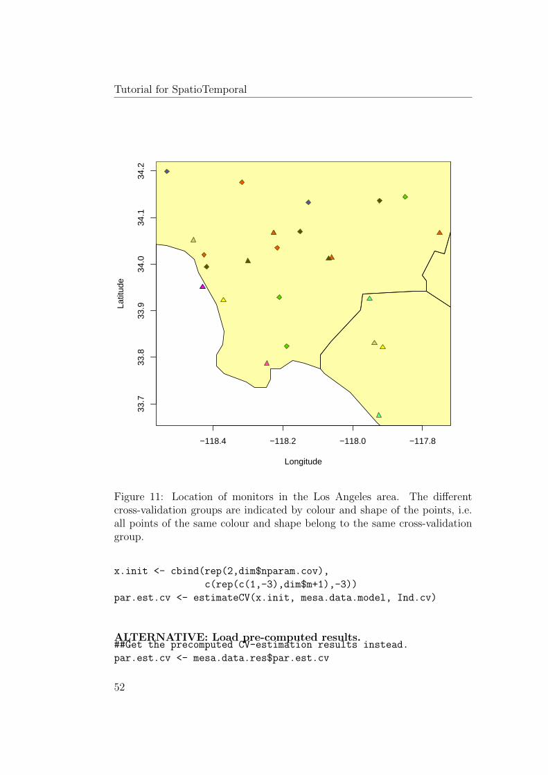
Tutorial for SpatioTemporal
−118.4 −118.2 −118.0 −117.8
33.7
33.8
33.9
34.0
34.1
34.2
Longitude
Latit
ude
Figure 11: Location of monitors in the Los Angeles area. The differentcross-validation groups are indicated by colour and shape of the points, i.e.all points of the same colour and shape belong to the same cross-validationgroup.
x.init <- cbind(rep(2,dim$nparam.cov),
c(rep(c(1,-3),dim$m+1),-3))
par.est.cv <- estimateCV(x.init, mesa.data.model, Ind.cv)
ALTERNATIVE: Load pre-computed results.##Get the precomputed CV-estimation results instead.
par.est.cv <- mesa.data.res$par.est.cv
52
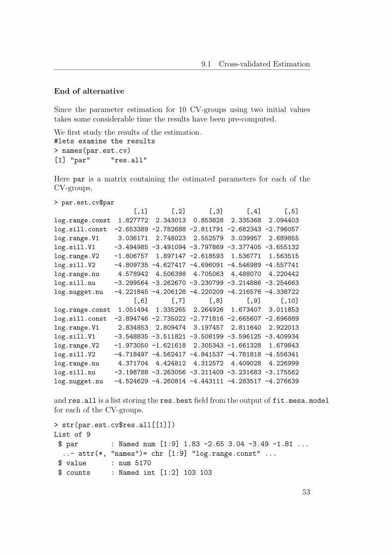
9.1 Cross-validated Estimation
End of alternative
Since the parameter estimation for 10 CV-groups using two initial valuestakes some considerable time the results have been pre-computed.
We first study the results of the estimation.#lets examine the results
> names(par.est.cv)
[1] "par" "res.all"
Here par is a matrix containing the estimated parameters for each of theCV-groups,
> par.est.cv$par
[,1] [,2] [,3] [,4] [,5]
log.range.const 1.827772 2.343013 0.853828 2.335368 2.094403
log.sill.const -2.653389 -2.782688 -2.811791 -2.682343 -2.796057
log.range.V1 3.036171 2.748023 2.552579 3.039957 2.689855
log.sill.V1 -3.494985 -3.491094 -3.797869 -3.377405 -3.655132
log.range.V2 -1.806757 1.897147 -2.618593 1.536771 1.563515
log.sill.V2 -4.809735 -4.627417 -4.696091 -4.546989 -4.557741
log.range.nu 4.578942 4.506398 4.705063 4.488070 4.220442
log.sill.nu -3.299564 -3.262670 -3.230799 -3.214886 -3.254663
log.nugget.nu -4.221845 -4.206128 -4.220209 -4.216576 -4.338722
[,6] [,7] [,8] [,9] [,10]
log.range.const 1.051494 1.335265 2.264926 1.673407 3.011853
log.sill.const -2.894746 -2.735022 -2.771816 -2.665607 -2.696889
log.range.V1 2.834853 2.809474 3.197457 2.811640 2.922013
log.sill.V1 -3.548835 -3.511821 -3.508199 -3.596125 -3.409934
log.range.V2 -1.973050 -1.621618 2.305343 -1.661328 1.679843
log.sill.V2 -4.718497 -4.562417 -4.841537 -4.781818 -4.556341
log.range.nu 4.371704 4.424812 4.312572 4.409028 4.226999
log.sill.nu -3.198788 -3.263056 -3.211409 -3.231683 -3.175562
log.nugget.nu -4.524629 -4.260814 -4.443111 -4.283517 -4.276639
and res.all is a list storing the res.best field from the output of fit.mesa.modelfor each of the CV-groups.
> str(par.est.cv$res.all[[1]])
List of 9
$ par : Named num [1:9] 1.83 -2.65 3.04 -3.49 -1.81 ...
..- attr(*, "names")= chr [1:9] "log.range.const" ...
$ value : num 5170
$ counts : Named int [1:2] 103 103
53
Tutorial for SpatioTemporal
..- attr(*, "names")= chr [1:2] "function" "gradient"
$ convergence: int 0
$ message : chr "CONVERGENCE: REL_REDUCTION_OF_F ..."
$ hessian : num [1:9, 1:9] -2.2384 1.4527 -0.0766 ...
$ conv : logi TRUE
$ par.init : Named num [1:9] 2 2 2 2 2 2 2 2 2
..- attr(*, "names")= chr [1:9] "log.range.const" ...
$ par.all : Named num [1:17] 3.8571 -0.2426 0.033 ...
..- attr(*, "names")= chr [1:17] "alpha.const.const" ...
Studying the conv-field in res.all
> sapply(par.est.cv$res.all,function(x) x$conv)
[1] TRUE TRUE TRUE TRUE TRUE TRUE TRUE TRUE TRUE TRUE
we see that all optimisations have converged for all CV-groups. The fieldpar.init gives information about which initial value gave the best optimi-sation result, for each CV-group
> sapply(par.est.cv$res.all,function(x) x$par.init)
[,1] [,2] [,3] [,4] [,5] [,6] [,7] [,8] [,9] [,10]
log.range.const 2 2 2 2 2 1 1 1 1 1
log.sill.const 2 2 2 2 2 -3 -3 -3 -3 -3
log.range.V1 2 2 2 2 2 1 1 1 1 1
log.sill.V1 2 2 2 2 2 -3 -3 -3 -3 -3
log.range.V2 2 2 2 2 2 1 1 1 1 1
log.sill.V2 2 2 2 2 2 -3 -3 -3 -3 -3
log.range.nu 2 2 2 2 2 1 1 1 1 1
log.sill.nu 2 2 2 2 2 -3 -3 -3 -3 -3
log.nugget.nu 2 2 2 2 2 -3 -3 -3 -3 -3
and we see that different initial values worked best for different CV-groups.
Finally we can study the difference in the estimated parameters for the dif-ferent CV-groups using a box-plot.
##Boxplot of the different estimates from the CV, see Figure 12
par(mfrow=c(1,1), mar=c(7,2.5,2,.5), las=2)
boxplot(t(par.est.cv$par))
points(par.est$res.best$par, pch=4, col=2)
The result in Figure 12, shows some considerable spread in the estimatedvariables, which can be compared to the parameter estimates based on allthe data in Figure 7.
54

9.2 Cross-Validated Prediction
●
●
log.
rang
e.co
nst
log.
sill.
cons
t
log.
rang
e.V
1
log.
sill.
V1
log.
rang
e.V
2
log.
sill.
V2
log.
rang
e.nu
log.
sill.
nu
log.
nugg
et.n
u
−4
−2
0
2
4
Figure 12: The estimated parameters for the 10 cross-validation groups, thered cross marks the parameter estimates obtained from the entire data inFigure 7, Section 8.1.
9.2 Cross-Validated Prediction
Once the parameters have been estimated, predictCV() does column-by-column predictions of the left-out observations denoted by TRUE in the Ind.cvdata set.
##Do cross-validated predictions using the newly
##estimated paremeters (takes roughly 1 minute)
> pred.cv <- predictCV(par.est.cv$par, mesa.data.model,
55

Tutorial for SpatioTemporal
+ Ind.cv, silent = FALSE)
[1] "Predicting cv-set 1/10"
[1] "Predicting cv-set 2/10"
[1] "Predicting cv-set 3/10"
[1] "Predicting cv-set 4/10"
[1] "Predicting cv-set 5/10"
[1] "Predicting cv-set 6/10"
[1] "Predicting cv-set 7/10"
[1] "Predicting cv-set 8/10"
[1] "Predicting cv-set 9/10"
[1] "Predicting cv-set 10/10"
This is done by computing the conditional expectation of the left-out observa-tions, as indicated in by the columns in Ind.cv, given all other observationsand the estimated parameters. The conditional expectation is computedunder the assumption that the observed and “unobserved” (i.e., left out) lo-cations follow a joint multivariate normal distribution characterised by theparameters we have estimated. Further details can be found in (Lindstromet al., 2011, Szpiro et al., 2010). It should be noted that the cross-validatedpredictions are conceptually identical to the predictions of unobserved loca-tions descriped in Appendix B.
We first examine the results of the predictions:
> names(pred.cv)
[1] "pred.obs" "pred.by.cv" "pred.all"
Here the pred.obs contains a data frame with predictions, prediction vari-ances and observations for each observed space-time location (this matchesthe observations in mesa.data.model$obs$obs)
> head(pred.cv$pred.obs)
obs pred pred.var
[1,] 4.577684 4.407115 0.14053531
[2,] 4.131632 4.518086 0.14223372
[3,] 4.727882 4.881646 0.09687876
[4,] 5.352608 5.110592 0.17340530
[5,] 5.281452 5.208341 0.08265215
[6,] 4.984585 4.864277 0.20100392
Since pred.obs only gives predictions at observed space-time locations thefull predictions are collected in the list pred.all
56
9.2 Cross-Validated Prediction
> str(pred.cv$pred.all[[1]])
num [1:280, 1:3, 1:3] 4.58 3.89 4.01 4.08 3.73 ...
- attr(*, "dimnames")=List of 3
..$ : chr [1:280] "1999-01-13" "1999-01-27" "1999-02-10" ...
..$ : chr [1:3] "60370002" "L002" "LC001"
..$ : chr [1:3] "obs" "pred" "pred.var"
Each element in the list contains a 3D-array with predictions, predictionvariances and observations for the sites left out in the corresponding CV-group.
Some standard cross-validation statistics can be obtained through:
> pred.cv.stats <- summaryStatsCV(pred.cv, lta=TRUE, trans=0)
> names(pred.cv.stats)
[1] "Stats" "res" "res.norm" "lta" "p"
Here summaryStatsCV computes prediction residuals, standardised residuals,cross-validation statistics, and the long term average at each site. Cross-validation statistics as well as the averages are computed on the natural scale(our observations are log NOx), with the exponential back-transformationbeing requested by the trans=0 option.
> pred.cv.stats$Stats
RMSE R2 coverage
obs 17.99432 0.7969228 0.9217828
lta 12.44381 0.5433923 NA
For cross-validation statistics the function gives us RMSE, R2, and the cover-age of the observations by a calculated 95% prediction intervals. The cross-validated statistics show a RMSE that is reasonably small, while the cross-validated R2 is reasonably large. Also, the 95% prediction intervals providecoverage that is close to 95%, at 0.922.
As discussed above, the cross-validation function predictCV leaves one siteout at a time and uses the estimated parameters to predict the left-out data.To assess the model’s predictive ability we plot four predicted time series(with 95% confidence intervals), and the left out observations (in red), shownin Figure 13.
##Plot observations with CV-predictions and
##95% prediction intervals, see Figure 13
par(mfcol=c(4,1),mar=c(2.5,2.5,2,.5))
57
Tutorial for SpatioTemporal
plotCV(pred.cv, 1, mesa.data.model)
plotCV(pred.cv, 10, mesa.data.model)
plotCV(pred.cv, 17, mesa.data.model)
plotCV(pred.cv, 22, mesa.data.model)
The object pred.cv contains the observations and predictions made usingpredictCV. Remember that this function takes our (number of observations)-by-(number of groups) data frame of logical values and predicts at the lo-cations and times denoted by TRUE. The function plotCV plots the observa-tions and predictions with corresponding 95% prediction intervals for eachlocation specified; this is what we are specifying by the integers in e.g.plotCV(pred.cv, 1, mesa.data.model). We can see the plots below:
In Figure 13 we can see that the observations lie reasonably close to thepredicted log NOx concentrations. The 95% prediction intervals also do agood job of covering the observations, and it seems the model has performedwell.
Another option is to do a scatter plot of the left out data against the predicted(points colour-coded by site), shown in Figure 14.
##Plot predicted vs. observed, see Figure 14par(mfcol=c(1,1),mar=c(4.5,4.5,2,2))
plot(pred.cv$pred.obs[,"obs"], pred.cv$pred.obs[,"pred"],
xlab="Observations", ylab="Predictions", pch=19,
cex=.1, col=mesa.data.model$obs$idx)
abline(0,1,col="grey")
Or a scatter plot of the average at each of the 25 sites against the predictedaverages, shown in Figure 15.
##Predicted long term average against observations
##(on the natural scale), see Figure 15par(mfcol=c(1,1),mar=c(4.5,4.5,3.5,2))
plot(pred.cv.stats$lta[,"obs"], pred.cv.stats$lta[,"pred"],
xlab="Observations", ylab="Predictions", main="Averages",
ylim=c(25,95), xlim=c(25,95))
abline(0,1,col="grey")
9.2.1 Residual Analysis
Before we start with a more thorough residual analysis, we need to create anindicator vector for which season each observation belongs to.
58

9.2 Cross-Validated Prediction
2000 2002 2004 2006 2008 2010
2.5
3.5
4.5
60370002
2000 2002 2004 2006 2008 2010
2.5
3.5
4.5
5.5
60371601
2000 2002 2004 2006 2008 2010
23
45
6
60590001
2000 2002 2004 2006 2008 2010
34
56
L002
Figure 13: Observed and predicted time series and 95% prediction intervalsat 4 locations
##create a vector dividing data into four seasons
I.season <- matrix(NA,length(mesa.data.model$obs$date),1)
I.season[months(mesa.data.model$obs$date) %in%
c("December","January","February"),1] <- "DJF"
I.season[months(mesa.data.model$obs$date) %in%
c("March","April","May"),1] <- "MAM"
I.season[months(mesa.data.model$obs$date) %in%
c("June","July","August"),1] <- "JJA"
I.season[months(mesa.data.model$obs$date) %in%
c("September","October","November"),1] <- "SON"
59
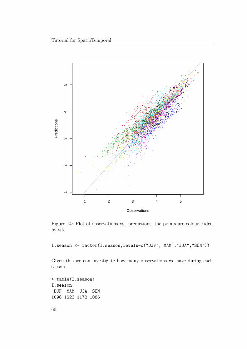
Tutorial for SpatioTemporal
●
●
●
●
●
●
●
●
●
●
●
●
●
●
●
●
●
●
●
●
●
●
●
●
●
●
●
●
●
●
●
●
●
●
●
●
●
●
●
●
●
●
●
●
●
●
●
●
●
●
●
●
●
●
●
●
●
●
●
●
●
●
●
●
●
●
●
●
●
●
●
●
●
●
●
●
●
●
●
●
●
●
●
●
●
●
●
●
●
●
●
●
●
●
●
●
●●
●
●
●
●●
●
●
●
●
●
●
●
●
●
●
●
●
●
●
●
●
●
●
●
●
●
●
●
●●
●
●
●
●
●
●
●
●
●
●
●
●
●
●
●
●
●
●
●
●
●
●
●
●
●
●
●●
●
●
●
●
●
●
●
●
●
●
●
●
●
●
●
●
●
●
●
●
●
●
●
●
●
●
●
●
●
●
●
●
●
●
●
●
●
●
●
●
●
●
●
●
●
●
●
●
●
●
●
●
●
●
●
●
●
●
●
●
●
●
●
●
●
●
●
●
●
●
●
●
●
●
●
●●
●
●
●
●
●
●
●
●
●
●
●
●
●
●
●
●
●
●
●
●
●
●
●
●
●
●
●
●
●
●
●
●
●
●
●
●
●
●
●
●
●
●
●
●
●
●
●
●
●
●
●
●
●
●
●
●
●
●
●
●
●
●
●
●
●
●
●
●
●
●
●
●
●
●
●
●
●
●
●
●
●
●
●
●
●
●
●
●
●
●
●
●
●
●
●
●
●
●
●
●
●
●
●
●
●
●
●
●
●
●
●
●
●
●
●
●
●
●
●
●
●
●
●
●
●
●
●
●
●
●
●●
●
●
●
●
●
●
●
●
●
●
●
●
●
●
●
●
●
●
●
●
●
●
●
●
●
●
●
●
●
●
●
●
●
●
●
●
●
●
●
●
●
●
●
●
●
●
●
●
●
●
●
●
●
●
●
●
●
●
●
●
●
●
●
●
●
●
●
●
●
●
●
●
●
●
●
●
●
●
●
●
●
●
●
●
●
●
●
●
●
●
●
●
●
●
●
●
●
●
●
●
●
●
●
●
●
●
●
●●
●
●
●
●
●
●
●
●
●
●
●
●
●
●
●
●
●
●
●
●
●
●
●
●
●
●
●
●
●
●
●
●
●
●
●
●
●
●
●
●
●
●
●
●
●
●
●
●
●
●
●
●
●
●
●
●
●
●
●
●
●
●
●
●
●
●
●
●
●
●
●
●
●
●
●
●
●
●
●
●
●
●
●
●
●
●
●
●
●
●
●
●
●
●
●
●
●
●
●●
●
●
●
●
●
●
●
●
●
●
●
●
●
●
●
●
●
●
●
●
●
●
●●
●
●
●
●
●
●
●
●
●
●
●
●
●
●
●
●
●
●
●
●
●
●
●
●
●
●
●
●
●
●
●
●
●
●
●
●
●
●
●
●
●
●
●
●
●
●
●
●
●
●
●
●
●
●
●
●
●
●
●
●
●
●
●
●
●
●
●
●
●
●
●
●
●
●
●
●
●
●
●
●
●
●
●
●
●
●
●
●
●
●
●
●
●
●
●
●
●
●●
●
●
●
●
●
●
●
●
●
●
●
●
●
●
●
●
●
●
●
●
●
●
●
●
●
●
●
●
●
●●
●
●
●
●
●
●
●
●●
●●
●
●
●●
●
●
●
●
●
●
●
●
●
●
●
●
●
●
●
●
●
●
●
●
●
●
●
●
●
●
●
●
●
●
●
●
●
●
●
●
●
●
●
●
●
●
●
●
●
●
●
●
●
●
●
●
●
●
●
●
●
●
●
●
●
●
●
●
●
●
●
●
●
●
●
●
●
●
●
●
●
●
●
●
●
●
●
●
●
●●
●
●
●
●
●
●
●
●
●
●
●
●
●
●
●
●
●
●
●
●
●
●
●
●
●
●
●
●
●
●
●
●
●
●
●
●
●
●
●
●
●
●
●
●
●
●
●
●
●●
●
●
●
●
●
●
●
●
●
●
●
●
●
●
●
●
●
●
●
●
●●
●
●
●
●
●
●
●
●
●
●
●
●
●
●
●
●
●
●
●
●
●
●
●
●
●
●
●
●
●
●
●
●
●
●
●
●
●
●
●
●
●
●
●
●
●
●
●
●
●
●
●
●
●
●
●
●
●
●
●
●
●
●
● ●
●
●
●
●
●
●
●
●
●
●
●
●
●
●
●
●
●
●
●
●
●
●
●
●
●
●
●
●
●
●
●
●
●
●
●
●
●
●
●
●
●
●
●
●
●
●
●
●
●
●
●
●
●
●
●
●
●
●
●
●
●
●
●
●
●
●
●
●
●
●
●
●
●
●
●
●
●
●
●
●
●
●
●
●
●
●
●
●
●
●
●
●
●
●
●
●
●
●
●
●
●
●
●
●
●
●
●
●
●
●
●
●
●
●
●
●
●
●
●
●
●
●
●
●
●
●
●
●
●
●
●
●
●
●
●
●
●
●
●
●
●
●
●
●
●
●
●
●
●
●
●
●
●
●
●
●
●
●
●
●
●
●
●
●
●
●
●
●
●
●
●
●
●
●
●
●
●
●
●
●
●
●
●
●
●
●
●
●
●
●
●
●
●
●
●
●
●
●
●
●
●
●
●
●
●
●
●
●
●●
●
●
●
●
●
●
●
●
●
●
●
●
●
●
●
●
●
●
●
●
●
●
●
●
●
●
●
●
●
●
●
●
●
●
●
●
●
●
●
●
●
●
●
●
●
●
●
●
●
●
●
●
●
●
●
●
●
●
●
●
●
●
●
●
●
●
●
●
●
●
●
●●
●
●
●
●
●
●
●
●
●
●
●
●
●
●
●
●
●
●
●
●
●
●
●
●
●
●
●
●
●
●
●
●
●
●
●●
●
●
●
●
●
●
●
●
●
●
●
●
●
●
●
●●
●
●
●
●
●
●
●
●
●
●
●
●
●
●
●
●
●
● ●
●
●
●
●
●
●
●
●
●
●
●
●
●
●
●
●
●●
●
●
●
●
●
●
●
●
●
●
●●
●
●
●
●
●
●
●
●
●
●
●
●
●
●
●
● ●
●
●
●
●
●
●
●
●
●
●
●
●
●
●
●
●
●
●
●
●
●
●
●
●
●
●
●
●
●
●
●
●
●
●
●
●
●
●
●
●
●
●
●
●
●
●
●
●
●
●
●
●
●
●●
●
●
●
●
●
●
●
●
●
●
●
●●
●
●
●
●
●
●
●
●
●
●
●
●
●
●
●
●
●
●
●
●
●
●
●
●
●
●
●
●
●
●
●
●
●
●
●
●
●
●
●
●
●
●
●
●●
●
●
●
●
●
●
●
●
●
●
●
●
●
●
●
●
●
●
●
●
●
●
●
●
●
●
●
●
●
●
●
●
●
●
●
●
●
●
●
●
●
●
●
●
●
●
●●
●
●
●
●
●
●
●
●
●
●
●
●
●
●
●
●
●
●
●
●
●
●
●
●
●
●
●
●
●
●
●
●
●
●
●
●
●
●
●
●
●
●
●
●
●
●
●
●●
●
●
●
●
●
●
●
●
●
●
●
●
●
●
●
●
●
●
●
●
●
●
●
●
●
●
●
●
●
●
●
●
●
●
●
●
●
●
●●
●
●
●
●
●
●
●
●
●
●
●
●
●
●
●
●
●
●
●
●
●
●
●
●
●●
●
●
●
●
●
●
●
●
●
●
●
●
●
●
● ●
●
●
●
●
●
●
●
●
●
●
●
●
●
●
● ●
●
●
●
●
●
●
●
●
●
●
●
●
●
●
●
●
●
●
●
●
●
●
●
●
●
●
●
●
●
●
●
●
●
●
●
●
●
●
●
●
●
●
●
●
●
●
●
●
●
●
●
●
●
●
●
●●
●
●
●
●
●
●
●
●
●
●
●
●
●
●
●
●
●
●
●
●
●
●
●
●
●
●
●
●
●
●
●
●
●
●
●
●
●
●
●
●
●
●
●
●
●
●
●
●
●
●
●●
● ●
●
●
●
●
●
●
●
●
●
●
●
●
●
●
●
●
●
●
●
●
●
●
●
●
●
●
●
●
●
●
●
●
●
●
●
●
●
●
●
●
●
●
●
●
●
●
●
●
●
●
●
●
●
●
●
●
●
●
●
●
●
●
●
●
●
●
●
●
●
●
●
●
●
●
●
●
●
●
●
●
●
●
●
●●
●
●
●
●
●
●
●
●
●
●
●
●
●
●
●
●
●
●
●
●
●
●
●
●
●
●
●
●
●
●
●
●
●
●
●
●●
●
●
●
●
●
●
●
●●
●
●
●
●
●
●
●
●
●
●
●
●
●
●
●
●
●
●
●
●
●
●
●
●
●
●
● ●
●
●
●
●
●
●
●
●
●
●
●
●
●
●
●
●
●
●
●
●
●
●
●
●
●
●
●
●
●
●
●●
●
●
●
●
●
●
●
●
●
●
●
●
●
●
●
●
●
●
●
●
●
●
●
●
●
●
●
●
●
●
●
●
●
●
●
●
●
●
●
●
●
●
●
●
●
●
●
●
●
●
●
●
●
●
●
●
●
●
●
●
●
●
●
●
●
●
●
●
●
●
●
●
●
●
●
●
●
●
●
●
●
●
●
●
●
●
●
●
●
●
●
●
●
●
●
●
●
●
●
●
●
●
●
●
●
●
●
●
●
●
●
●
●
●
●
●
●
●
●
●
●
●
●
●
●
●
●
●
●
●
●
●
●
●
●
●
●
●
●
●●
●
●
●
●
●
●
●
●
●
●
●
●
●
●
●
●
●
●
●
●
●
●
●
●
●
●
●
●
●
●
●
●
●
●
●
●
●
●
●
●
●
●
●
●
●
●
●
●
●
●
●
●
●
●
●
●
●
●
●
● ●
●
●
●
●
●
●
●
●
●
●
●
●
●
●
●●
●
●
●
●
●
●
●
●
●
●
●
●
●
●
●
●
●
●
●
●
●
●
●
●
●
●
●
●
●
●
●
●
●
●
●
●
●
●
●
●
●
●
●●
●
●
●
●
●
●
●
●
●
●
●
●
●
●
●
●
●
●
●
●
●
●
●
●
●
●
●
●
●
●
●
●
●
●
●
●
●
●
●
●
●
●
●
●
●
●
●
●
●
●
●
●
●
●
●
●
●
●
●
●
●
●
●
●
●
●
●
●
●
●
●
●
●
●
●
●
●
●
●
●
●
●
●
●
●
●
●
●
●
●
●
●
●
●●
●
●
●
●
●
●
●
●
●
●
●
●
●
● ●
●
●
●
●
●
●
●
●
●
●
●
●
●
●
●
●
●
●
●
●
●
●
●
●
●
●
●
●
●
●
●
●
●
●
●
●
●
●
●
●
●
●
●
●
●
●
●
●●
●
●
●
●
●
●
●
●
●
●
●
●
●
●
●
●
●
●
●
●
●
●
●
●
●
●
●
●
●
●
●
●
●
●
●
●
●
●
●
●●
●
●
●
●
●
●
●
●
●
●
●
●
●
●
●
●
●
●
●
●
●
●
●
●
●
●
●
●
●
●
●
●
●
●
●
●
●
●
●
●
●
●
●●
●
●
●
●
●
●
●
●
●
●
●
●
●
●
●●
●
●
●
●
●
●
●
●
●
●
●
●
●
●
●
●
●
●
●
●
●
●
●
●
●
●
●
●
●
●
●
●
●
●
●
●
●
●
●
●
●
●
●
●
●
●
● ●
●
●
●
●
●
●
●
●
●
●
●
●
●
●
●
●
●
●
●
●
●
●
●
●
●
●
●
●
●
●
●
●
●
●
●
●
●
●
●
●
●
●
●
●
●
●
●
●
●
●
●
●
●
●
●
●
●
●
●
●
●
●
●
●
●
●
●
●
●
●
●
●
●
●
●
●
●
●
●
●
●
●
●
●●
●
●
●
●
●
●
●
●
●
●
●
●
●
●
●
●
●
●
●
●
●
●
●
●
●
●
●
●
●
●
●
●
●
●
●
●
●
●
●
●
●
●
●
●
●
●
●
●
●
●
●
●
●
●
●
●
●
●
●
●
●
●●●
●
●
●
●
●
●
●
●
●
●
● ●
●
●
●
●
●
●
●
●
●
●
●
●
●
●
●
●
●
●
●
●
●
●
●
●
●
●
●
●
●
●
●
●
●
●
●
●
●
●
●
●
●
●
●
●
●
●
●
●
●
●
●●
●
●
●
●
●
●
●
●
●
●
●
●
●●
●
●
●
●
●●
●
●
●
●
●
●
●
●
●
●
●
●
●
●
●
●
●
●
●
●
●
●
●
●
●
●
●
●
●
●
●
●
●
●
●●
●
●
●
●
●
●
●
●
●
●
●
●
●
●
●
●
●
●
●●
●
●
●
●
●
●
●
●
●
●
●
●
●
●
●
●
●
●●
●
●
●
●
●
●
●
●
●
●
●
●
●
●
●
●
●
●
●●
●
●
●
●
●
●
●
●
●
●
●
●
●
●
●
●
●
●
●
●
●
●
●
●
●
●
●
●
●
●
●
●
●
●
●
●
●
●
●
●
●
●
●
●
●
●
●
●
●
●
●
●
●
●
●
●
●
●
●
●
●
●
●
●
●
●
●
●
●
●
●
●
●
●
●
●
●
●
●
●
●
●
●
●
●
●
●
●
●
●
●
●
●
●
●
●
●
●
●
●
●
●
●
●
●
●
●
●
●
●
●
●
●
●
●
●
●
●
●
●
●
●
●
●
●
●
●
●
●
●
●
●
●
●
●
●
●
●
●
●
●
●
●
●
●
●
●
●
●
●
●
●
●
●
●
●
●
●
●
●
●
●
●
●
●
●
●
●
●
●
●
●
●
●
●
●
●
●
●
●
●
●
●
●
●
●
●
●
●
●
●
●
●
●
●
●
●
●
●
●
●
●
●
●
●●
●
●
●
●
●●
●
●
●
●
●
●
●
●
●
●
●
●
●
●
●
●
●
●
●
●
●
●
●
●
●
●
●
●
●
●
●
●●
●
●
●
●
●
●
●
●
●
●
●
●
●
●
●
●
●
●
●
●
●
●
●
●
●
●
●
● ●
●
●
●
●
●
●
●
●
●
●
●
● ●
●
●
●
●
●
●
●
●
●
●
●
●
●
●
●
●
●
●
●
●
●
●
●
●
●
●
●
●
●
●
●
●
●
●
●
●
●
●
●
●
●
●
●
●
●
●
●
●
●
●
●
●
●
●
●
●
●
●
●
●
●
●
●
●
●
●
●
●
●
●
●
●
●
●
●
●
●
●
●
●
●
●
●
●
●
●
●
●
●
●
●
●
●
●
●
●
●
●
●
●
●
●
●
●
●
●
●
●
●●
●
●
●
●
●
● ●
●
●
●
●
●
●
●
●
●
●
●
●
●
●
●
●
●
●
●
●
●
●
●
●
●
●
●
●
●
●
●
●
●
●
●
●
●
●
●
●
●
●
● ●
●
●
●
●
●
●
●
●
●
●
●
●
●
●
●
●
●
●
●
●
●
●
●
●
●
●
●
●
●
●
●
●
●
●
●
●
●
●
●
●
●
●
●
●
●
●
●
●
●
●
●
●
●
●
●
●
●
●
●
●
●
●
●
●●
●
●
●
●
●
●
●
●
●
●
●
●
●
●
●
●
●
●
●
●
●
●
●
●
●
●
●
●
●
●
●
●
●
●
●
●
●
●
●
●
●
●
●
●
●
●
●
●
●
●
●
●
●
●
●
●
●
●
●
●
●
●
●
●
●
●
●
●
●
●
●
●
●
●
●
●
●
●
●
●
●
●
●
●
● ●
●
●
●
●
●
●
●
●
●
●
●
●
●
●
●
●
●
●
●
●
●
●
●
●
●
●
●
●
●
●
●
●
●
●
●
●
●
●
●
●
●
●
●
●
●
●
●
●
●
●
●
●
●
●
●
●
●
●
●
●
●
●
●
●
●
●
●
●
●
●
●
●
●
●
●
●
●
●
●
●
●
●
●
●
●
●
●
●
●
●
●
●
●
●
●
● ●
●
●
●
●
●
●
●
●
●
●
●
●
●
●
●
●●
●
●
●
●
●
●
●
●
●
●
●
●
●
●
●
●
●
●
●
●
●
●
●
●
●
●
●
●
●
●
●
●
●
●
●
●
●
●
●
●
●
●
●
●
●
●
●
●
●
●
●
●
●
●
●
●
●
●
●
●
●
●
●
●
●
●
●
●
●
●
●
●
●
●
●
●
●
●
●
●
●
●
●
●
●
●
●
●
●
●
●
●
●
●
●
●
●
●
●
●
●
●
●
●
●
●
●
●
●
●
●
●
●
●
●
●
●
●
●
●
●
●
●
●
●
●
●
●
●
●
●
●
●
●
●
●
●
●
●
●
●
●
●
●
●
●
●
●
●
●
●
●
●
●
●
●
●
●
●
●
●
●
●
●
●
●
●
●
●
●
●
●
●
●
●
●●
●
●
●
●
●
●
●
●
●
●
●
●
●
●
●
●
●
●●
●
●
●
●
●
●
●
●
●●
●
●
●
●
●
●
●
●
●
● ●
●
●
●
●
●
●
●
●
●
●
●
●
●
●
●
●
●
●
●
●
●
●
●
●
●
●
●
●
●
●
●
● ●
●
●
●
●
●
●
●
●
●
●
●
●
●
●
●
●
●
●
●
●
●
●
●
●
●
●
●
●
●
●
●
●
●●
●
●
●
●
●
●
●
●
●
●
●●
●
●
●
●
●
●
●
●
●
●
●
●
●
●
●
●
●
●
●
●
●
●
●
●
●
●
●
●
●
●
●●
●
●
●
●
●
●
●
●
●
●
●
●
●
●●
●
●
●
●
●
●
●
●
●
●
●
●
●
●
●
●
●
●
●
●
●
●
●
●
●
●
●
●
●
●
●
●
●
●
●
●
●
●
●
●
●
●
●
●
●
●
●
●
●
●
●
●
●
●
●
●
●
●
●
●
● ●
●
●
●
●
●
●
●
●
●
●
●
●
●
●
●
●
●
●
●
●
●
●
●
●
●
●
●
●
●
●
●
●
●
●
●
●
●
●
●
●
●
●
●
●
●
●
●
●
●
●
●
●
●
●
●
●
●
●
●
●
●
●
●
●
●
●
●
●
●
●
●
●
●
●
●
●
●
●
●
●
●
●
●
●
●
●
●
●
●
●
●
●●
●
●
●
●
●
●
●
●
●
●
●
●
●
●
●
●
●
●
●
●
●
●
●
●
●
●
●
●
●
●
●
●
●
●
●
●
●
●
●
●
●
●
●
●
●
●
●
●
●
●
●
●
●
●
●
●
●
●
●
●
●
●
●
●
●
●
●
●
●
●
●
●
●
●
●
●
●
●
●
● ●
●
●
●
●
●
●
●
●
●
●
●
●
●
●
●
●
●
●
●
●
●
●
●
●●
●
●
●
●
●
●
●
●
●
●
●
●
●
●
●
●
●
●
●
●
●
●
●
●
●
●
●
●
●
●
●
●
●
●
●
●
●
●
●
●
●
●
●
●
●
●
●
●
●
●
●
●
●
●
●
●
●
●
●
●
●
●
●
●
●
●
●
●
●
●
●
●
●
●
●
●
●
●
●
●
●
●
●
●
●
●
●
●
●
●
●
●
●
●
●
●
●
●
●
●
●
●
●
●
●
●
●
●
●
●
●
●
●●
●
●
●
●
●
●
●
●
●
●
●
●
●
●
●
●
●
●
●
●●
●
●
●
●
●
●
●
●●
●
●
●
●
●
●
●
●
●
●
●
●
●
●
●
●
●
●
●
●
●
●
●
●
●
●●
●
●
●
●
●
●
●
●
●
●
●
●
●
●
●
●
●
●
●
●
●
●
●●
●
●
●
●
●
●
●
●
●
●
●
●
●
●
●
●
●●
●
●
●
●
●
●
●
●
●
●
●
●
●
●
●
●
●
●
●
●
●
●
●
●
●
●
●
●
●
●
●
●
●
●
●
●
●
●
●
●
●
●
●
●
●
●
●
●
●
●
●
●
●
●
●
●
●
●
●
●
●
●
●
●
●
●
●
●
●
●
●
●
●
●
●
●
●
●
●
●
●
●
●
●
●
●
●
●
●
●
●
●
●
●
●
●
●
●
●
●
●
●
●
●
●
●
●
●
●
●
●
●
●
●
●
●
●
●
●
●
●
●
●
●
●
●
●
●
●
●
●●
●
●
●
●
●
●
●
●
●
●
●
●
●●
●
●
●
●
●
●
●
●
●
●
●
●
●
●
●
●
●
●
●
●
●
●
●
●
●
1 2 3 4 5
12
34
5
Observations
Pre
dict
ions
Figure 14: Plot of observations vs. predictions, the points are colour-codedby site.
I.season <- factor(I.season,levels=c("DJF","MAM","JJA","SON"))
Given this we can investigate how many observations we have during eachseason.
> table(I.season)
I.season
DJF MAM JJA SON
1096 1223 1172 1086
60
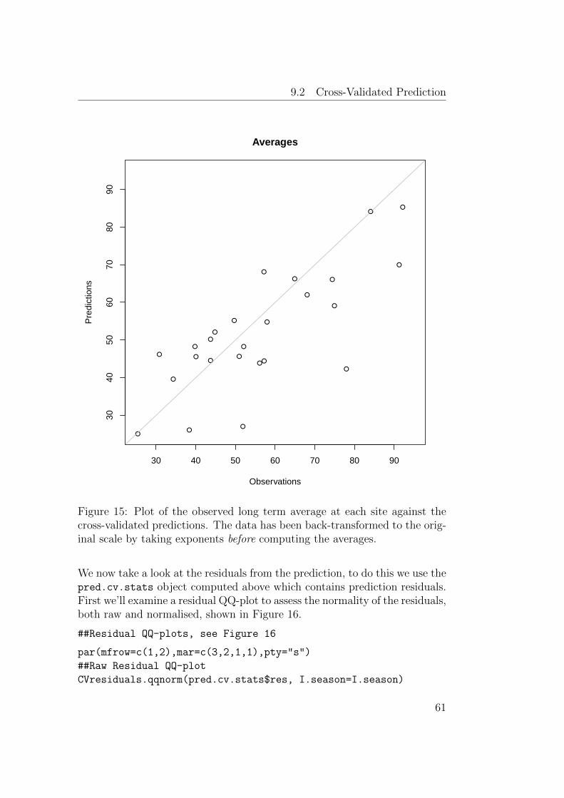
9.2 Cross-Validated Prediction
●●
●
●
●
●
●
●
●
●
●
●
●
●
●
●
●
●
●
●
●
●
●
●
●
30 40 50 60 70 80 90
3040
5060
7080
90
Averages
Observations
Pre
dict
ions
Figure 15: Plot of the observed long term average at each site against thecross-validated predictions. The data has been back-transformed to the orig-inal scale by taking exponents before computing the averages.
We now take a look at the residuals from the prediction, to do this we use thepred.cv.stats object computed above which contains prediction residuals.First we’ll examine a residual QQ-plot to assess the normality of the residuals,both raw and normalised, shown in Figure 16.
##Residual QQ-plots, see Figure 16
par(mfrow=c(1,2),mar=c(3,2,1,1),pty="s")
##Raw Residual QQ-plot
CVresiduals.qqnorm(pred.cv.stats$res, I.season=I.season)
61

Tutorial for SpatioTemporal
##Normalized Residual QQ-plot
CVresiduals.qqnorm(pred.cv.stats$res.norm, norm=TRUE,
I.season=I.season)
Here we have used the I.season indicator to colour code our observations,this should help us to detect any seasonal effects on the predictions.
●
●
●
●
●●●
●
●
●
●
●
●●●
●
●
●
●
●
●
●
●
●
●
●
●
●
●●●
●
●
●
●
●
●
●
●
●
●●
●
●●
●
●
●
●
●
●
●
●
●
●●
●●●
●
●
●
●●
●
●
●
●
●
●
●
●●
●
●
●●
●
●●
●
●
●
●
●
●●
●
●
●
●
●
●
●●
●
●
●
●
●
●●
●
●
●●
●
●●
●
●
●
●
●
●
●●
●
●
●●
●
●
●
●
●
●
●
●
●
●
●●
●
●●
●
●
●
●
●
●●
●
●
●●
●
●●
●
●
●
●
●
●●
●
●
●
●
●
●
●
●
●●
●
●
●
●
●
●
●
●
●
●
●
●●
●
●
●
●
●
●
●
●
●
●
●
●
●
●●
●
●
●
●
●
●
●
●
●
●
●
●●
●
●●
●
●
●
●
●
●
●
●
●●
●
●
●
●
●
●
●
●
●
●
●
●
●
●
●
●
●
●
●
●
●
●
●
●
●
●
●
●
●●
●
●
●
●
●
●
●
●
●
●
●
●
●●
●
●
●
●
●
●
●
●
●
●
●●
●
●
●●
●
●
●●
●●
●
●
●●
●
●
●●
●
●
●
●●●
●
●
●
●●
●●
●
●
●
●●
●●
●
●
●
●
●
●
●
●
●
●
●
●●●●
●
●
●
●
●
●
●
●
●
●
●
●
●●
●
●
●●
●
●
●
●
●
●
●●
●
●
●
●
●●
●
●
●
●
●
●●●●
●
●
●
●●●
●
●
●
●
●
●
●
●●●
●
●
●●
●
●
●
●
●
●
●●
●●
●
●
●
●●
●
●
●
●
●
●
●●
●
●
●
●
●
●●
●
●●
●
●
●●
●
●●
●
●
●
●●
●
●
●
●
●
●●
●●
●●
●
●●
●
●
●
●
●
●
●
●●
●
●
●
●
●●
●
●
●
●
●
●
●
●●
●
●●
●
●
●●
●
●
●
●
●
●
●●
●
●●
●
●●
●
●
●
●
●
●
●●
●
●
●●
●
●
●●
●
●●
●
●
●
●●
●
●
●●
●●
●
●
●
●
●
●
●
●●
●
●
●
●
●
●
●
●
●●
●
●
●
●●
●
●
●●
●
●
●
●
●
●
●
●
●
●●
●
●
●●
●
●
●
●
●●
●
●
●
●●
●
●
●●●
●
●
●
●
●
●
●
●
●●
●
●
●
●
●
●
●
●
●●
●
●
●
●●
●
●
●
●
●
●
●
●
●
●
●
●
●
●●
●
●
●
●
●
●●
●
●●
●
●
●
●●
●
●
●
●
●●
●
●●
●
●
●●
●
●
●
●
●
●●
●
●
●
●
●
●
●
●
●
●
●
●
●●
●
●●
●
●
●
●●
●
●
●
●●
●
●
●
●
●
●
●
●
●●●
●
●
●●●
●
●
●
●
●
●●
●●
●
●
●●
●
●
●
●
●
●
●
●
●●
●
●
●●
●
●
●
●
●
●
●
●
●●●
●
●
●●
●●
●
●
●●
●
●●
●
●
●
●
●●
●
●
●
●
●
●
●●●●
●
●
●
●●
●
●
●
●
●
●
●
●●
●
●
●
●
●●
●
●
●
●
●
●●●●
●
●
●
●
●●
●
●
●
●
●
●●
●●●
●
●
●●
●●
●
●
●
●
●
●●●
●
●
●
●
●●
●●
●
●
●
●
●
●
●
●
●
●●
●
●
●●●
●
●
●
●
●
●
●●
●
●●
●
●
●
●●
●
●●
●
●
●
●●
●
●●
●
●
●●
●
●
●●
●
●
●
●
●
●
●●
●●
●●
●
●
●
●
●
●
●
●
●
●
●●●
●
●
●
●
●
●
●
●
●
●
●
●
●
●●
●
●
●
●
●
●
●
●
●
●
●
●
●
●●
●
●
●●
●
●
●
●●
●
●
●
●
●
●●●
●
●
●
●
●
●
●
●
●
●
●
●
●
●●
●●
●
●
●
●
●
●
●
●
●
●
●
●
●●●
●
●●
●
●
●
●
●
●
●
●
●
●●
●
●
●
●
●
●
●●
●
●
●
●
●
●
●●●
●
●
●●
●
●
●
●
●
●
●
●●
●
●
●
●
●
●
●
●●
●●
●
●
●
●
●
●
●
●
●
●
●
●
●
●
●●
●
●●
●
●
●
●
●●
●
●
●
●
●
●
●●●●
●●
●
●
●
●●●
●
●
●
●●
●
●●
●●
●
●
●
●
●
●
●●●
●●
●
●
●
●
●
●●
●●
●
●●●
●●●
●
●
●
●
●
●
●
●●
●
●
●
●
●
●
●●
●●
●
●
●
●
●
●
●
●
●
●
●
●
●
●
●●
●●
●
●
●
●
●
●
●●
●
●
●
●
●
●●●
●
●
●
●
●
●
●
●
●●
●
●
●
●
●
●●
●●●
●
●
●
●
●
●●
●●
●
●
●
●●
●
●●
●
●
●
●
●
●
●
●
●●
●
●●
●●
●
●●
●
●
●
●●
●●
●●
●
●
●
●●
●●
●●
●
●
●
●
●●
●
●●
●
●
●●
●●●
●●
●
●
●
●●
●
●
●●
●
●
●
●●
●
●
●●●●
●
●●
●●
●
●
●
●
●
●
●●
●
●
●●
●
●
●●
●
●
●●
●
●
●
●
●●
●
●●
●
●
●
●
●
●
●
●
●
●
●
●
●
●●
●
●●
●
●
●
●
●
●
●
●●
●
●
●
●●
●
●
●●
●●
●
●●
●
●
●
●
●
●
●
●●
●
●
●●
●
●
●
●
●
●
●
●
●
●
●
●
●
●
●●●
●
●●
●●
●
●
●
●
●
●●●
●
●
●●
●
●
●
●●
●
●
●
●
●
●
●●
●
●
●
●
●
●
●
●●
●●
●
●
●
●
●●
●
●
●
●
●●
●
●
●●
●
●
●
●
●●
●
●
●●
●
●
●●
●●
●
●
●
●●
●
●
●
●●
●
●●
●
●
●
●●
●
●
●
●
●●
●●
●●
●
●
●
●●
●
●
●
●
●●
●
●
●●
●
●
●●
●
●●
●
●
●●
●
●●
●
●
●
●
●
●
●
●●
●
●
●
●●
●
●
●
●
●
●
●
●●●●
●●
●
●
●
●
●
●
●
●
●
●
●
●●
●●
●
●
●
●●
●
●
●
●
●
●
●
●●
●●●
●
●
●●●
●
●
●
●●●●
●●
●
●
●
●●
●
●
●
●
●
●
●●
●
●●
●
●
●
●●
●
●
●
●
●
●
●●●
●●
●
●
●
●
●●
●
●
●
●●
●●●
●●
●
●
●
●
●
●
●
●
●
●●
●●
●
●●
●
●
●
●●
●
●
●
●
●●●●●
●
●
●
●
●
●●●
●
●
●
●●
●●
●●
●
●
●
●
●
●
●
●●
●
●●●
●●
●
●
●
●
●●●
●
●●
●
●
●
●●●
●
●
●
●
●●
●
●
●
●
●
●●●●
●
●
●
●
●
●●
●
●●
●
●
●
●
●●
●
●
●
●
●●●
●
●
●
●
●
●
●●
●
●
●●
●●
●
●
●
●●
●
●
●●
●●●
●●●
●●●
●
●
●
●
●
●
●
●●●
●●
●
●●
●●
●●
●
●
●
●●●
●
●●
●
●●
●
●●
●
●
●
●
●
●
●
●●●
●
●
●
●
●
●
●
●
●
●
●●
●
●
●
●
●
●
●
●
●
●
●
●●
●●
●
●
●
●
●
●●
●
●●
●
●
●
●
●
●●
●
●
●●
●
●
●
●
●
●
●
●
●●
●
●
●●●
●
●
●
●●
●
●●●●●
●●●
●
●
●
●
●
●
●
●●
●
●●●
●●
●
●
●
●
●
●●
●●
●
●●●
●
●●
●
●
●
●
●●
●
●
●
●●●
●●
●
●
●
●
●
●●
●
●
●
●
●●
●
●
●
●
●
●
●
●
●●
●
●
●●
●
●
●
●
●
●
●
●
●●
●
●●
●
●●
●
●
●
●
●
●
●
●
●
●
●
●
●
●
●●
●
●
●
●
●●
●●
●
●
●
●●
●
●
●
●
●●
●●
●
●
●
●
●●
●
●
●
●
●
●
●
●
●●
●
●
●
●
●
●
●
●
●
●
●
●●
●●
●
●
●
●●
●
●●
●
●
●
●
●
●
●●
●
●
●●
●●
●
●
●
●
●●
●
●●
●
●●
●
●●
●
●
●
●
●
●
●
●
●●
●
●
●●
●
●
●●
●
●
●
●
●
●
●
●
●
●
●
●
●
●●
●
●●●
●
●●
●
●●
●
●
●
●
●●
●
●
●
●
●
●
●
●
●
●
●
●
●
●
●
●
●
●
●
●
●
●
●
●
●
●
●
●
●
●
●
●
●
●
●
●
●
●
●
●
●
●
●
●
●
●
●
●●
●
●
●
●●
●
●
●
●
●●
●
●●
●●
●
●
●
●
●
●
●
●
●●
●
●
●
●●
●
●
●●
●
●
●
●
●
●
●
●
●●
●
●
●
●
●
●
●
●
●
●
●
●
●
●●
●
●
●●
●
●
●
●●
●
●
●●
●
●
●
●●
●
●
●●
●
●
●
●
●●●
●
●●
●
●
●●
●●
●
●
●
●
●●
●●
●
●
●
●
●
●
●●
●
●
●
●●
●
●●
●
●
●●
●
●
●
●
●
●
●●
●
●
●
●
●
●
●
●●
●
●
●
●
●●
●
●
●
●
●
●
●●●
●
●
●
●
●
●●
●
●
●●
●
●
●●
●
●
●
●
●
●
●
●
●
●
●
●
●
●
●
●
●
●
●●
●
●
●
●
●
●
●
●
●
●
●
●
●●
●
●●
●
●
●
●
●
●●
●
●
●
●●
●
●
●
●
●
●
●
●
●
●
●●
●
●
●
●
●●
●
●
●
●
●●
●
●
●
●
●
●
●
●
●
●
●
●
●
●
●
●
●
●
●
●●
●
●
●
●
●
●
●
●
●
●
●
●
●
●●
●
●
●
●
●
●
●●
●
●
●
●
●●
●
●
●●
●
●
●
●
●
●
●
●
●
●●
●
●
●●
●
●
●
●
●
●
●●
●
●●
●
●
●
●
●
●
●
●
●
●●
●
●
●
●
●
●
●
●
●
●
●
●
●
●
●
●
●
●
●
●
●
●
●
●
●
●
●●
●
●
●
●
●
●
●
●
●
●
●●
●
●●
●
●
●●
●
●
●
●
●
●●●
●
●
●
●
●●
●
●
●
●
●
●●●●
●
●●
●●
●
●
●
●
●
●●
●●
●
●●
●●
●
●
●
●
●
●●
●
●●
●●
●
●
●
●
●●
●
●●
●
●●
●
●
●
●
●
●
●●
●
●●
●
●●
●
●
●
●
●
●
●
●
●
●●
●
●
●●
●
●
●
●
●
●
●●
●●
●●
●
●
●
●
●
●
●
●
●●
●●
●●
●●
●
●
●
●
●●
●
●
●
●
●
●
●
●
●
●
●
●
●
●
●
●●
●
●
●
●
●●
●
●
●
●
●
●
●●●●
●●
●
●
●●
●
●
●
●●
●●
●
●●
●
●
●
●
●
●
●
●
●
●●
●●●
●
●
●
●
●
●
●
●●
●●
●
●
●
●●
●
●
●
●
●●●
●
●
●
●
●
●●
●
●
●
●
●
●●
●
●
●
●
●
●●
●
●
●
●
●
●
●●
●
●
●●
●●
●
●
●
●
●●
●
●
●●●
●
●
●●
●
●●
●
●
●
●
●
●
●
●
●
●●
●
●
●
●
●●
●●
●
●
●
●
●
●
●
●
●
●●
●
●
●
●●●
●●●
●
●●
●
●
●
●
●
●●
●●
●
●
●●●●●
●
●
●
●
●
●
●●
●
●
●
●
●
●
●
●●
●
●
●
●
●●
●
●
●●
●●
●●
●
●
●
●●
●
●●
●
●●
●
●
●●
●
●●
●
●●
●●
●●
●●
●
●●
●
●
●●
●●
●●
●
●
●●
●●
●
●
●
●
●
●
●
●
●●
●●
●
●
●
●
●●
●
●●
●
●
●
●
●
●
●
●
●
●●
●
●
●
●
●●
●●
●●
●
●
●
●
●
●
●
●
●●
●
●
●
●
●
●●
●
●
●
●
●
●
●
●
●
●
●
●
●
●
●
●●
●
●
●
●
●
●
●
●
●
●●
●●
●
●
●●
●
●
●●
●
●
●●
●●
●
●
●●
●●
●
●
●
●●
●
●●
●
●●●
●
●
●●●
●●
●
●
●
●●
●
●
●
●
●
●
●●
●
●
●
●
●
●
●●
●
●
●●
●
●
●
●
●
●●
●●
●
●●
●
●
●●
●
●
●●
●
●
●
●
●●
●●
●
●●●
●
●
●●
●
●●
●●●●
●
●●
●●
●
●
●
●
●●
●
●
●
●
●
●
●
●●
●
●●
●●●
●●
●
●●
●●
●
●
●
●
●
●●
●
●●●●
●
●
●
●
●
●●
●
●
●
●
●●
●●●
●
●
●
●
●●
●
●
●
●
●
●
●
●
●
●
●●
●●
●●
●
●
●●●
●
●
●
●
●
●●●
●●
●
●●
●
●
●
●
●
●
●
●●
●
●
●●
●
●
●●●
●●
●●
●
●
●●
●
●●
●
●
●
●
●●
●●●
●●
●
●
●
●
●●
●
●
●
●
●
●
●
●
●
●●●
●●
●
●
●
●
●
●
●
●
●
●
●
●
●
●
●
●●●
●●
●
●
●●
●●
●
●
●
●
●
●
●
●
●
●●
●●
●
●●
●
●
●●
●
●
●
●
●●
●●
●
●
●●
●
●
●●
●
●●●
●
●●
●
●
●
●
●
●
●●
●
●
●
●
●
●
●
●
●●
●
●
●
●
●
●
●
●
●
●
●
●
●
●●
●●●
●
●
●
●●
●
●●
●
●●
●●
●
●●
●
●●
●
●
●
●
●
●
●●
●
●
●●
●
●
●
●●
●●
●
●
●
●
●
●
●
●
●
●
●
●
●
●●
●●
●
●●
●●
●
●●
●
●
●●
●
●
●●
●●
●●
●
●
●●
●
●
●
●
●
●●
●
●
●
●●
●
●
●
●●
●
●●
●
●●
●
●
●●
●
●
●●●
●●
●
●●
●●●
●
●●
●
●
●●
●
●
●
●●
●
●●
●
●
●●
●
●
●
●
●
●
●
●
●
●
●●●
●
●●
●
●
●●
●
●●
●
●
●
●●
●
●●
●
●
●
●
●
●
●
●●●●
●
●
●
●●
●
●
●
●
●
●●
●
●
●●
●
●●
●
●
●
●●
●●
●
●
●
●
●
●
●●
●
●
●
●
●
●
●●
●
●●●
●●
●
●
●●
●●
●●
●
●
●
●●
●●
●●
●
●
●
●●
●
●
●
●
●
●
●
●
●●
●●●
●●●
●●
●
●
●●
●
●
●
●
●
●
●
●●●
●
●
●
●●
●●
●
●
●
●●
●●●
●
●
●
●
●●
●
●
●
●
●
●●●
●
●●
●
●●
●
●
●
●
●●
●
●
●
●
●
●
●
●
●
●
●
●
●●
●●
●
●
●●
●
●
●
●
●
●●●
●
●●
●
●●
●●
●
●
●
●
●
●
●
●
●●●●
●
●●
●
●●
●●
●
●
●●
●
●●
●
●●
●●
●
●●●
●
●
●●
●
●
●●
●
●●
●
●●
●●
●
●●●
●●
●●
●
●
●●
●
●
●
●
●
●
●
●
●●●
●●
●
●
●
●
●●
●
●
●
●
●
●●
●
●
●●
●
●
●
●●
●
●●
●
●
●
●
●
●
●
●●
●
●●
●
●
●●
●
●
●●
●
●
●
●
●
●●
●
●
●
●
●
●
●●●
●●
●
●
●
●
●
●
●
●
●
●●
●●
●●
●
●
●●
●
●
●
●
●
●
●●
●
●
●
●●
●
●
●
●●
●
●
●
●
●
●
●
●
●
●
●●
●
●●
●
●
●
●●●
●
●●
●
●
●
●
●
●
●
●
●
●
●●
●
●
●●
●
●
●
●
●
●
●
●
●
●
●●
●
●
●
●
●
●●
●●
●
●
●
●
●
●
●
●
●
●
●●
●
●
●
●
●●●
●
●
●
●
●
●
●
●
●
●
●
●
●
●
●
●
●
●
●●
●●
●
●
●
●
●
●●
●
●●●
●
●
●
●
●●●
●
●●
●
●
●
●
●
●
●●●
●
●
●
●
●
●
●●
●
●
●
●
●
●●
●
●
●●
●
●
●
●
●
●
●
●●
●
●
●
●
●
●
●●
●
●
●●
●
●
●●
●
●
●
●
●
●
●
●
●
●●
●
●●
●
●
●
●
●
●
●
●●
●
●
●
●
●
●●
●
●●
●
●●
●
●
●●
●●●
●
●
●
●
●
●
●
●●
●
●
●●
●
●
●●●
●
●
●
●
●●●
●
●
●●
●
●●
●
●
●●
●
●●
●
●
●
●
●●
●
●
●
●
●
●●●
●
●
●
●●
●
●
●
●
●●
●
●
●
●
●
●
●
●
●
●
●
●●
●
●
●
●
●●
●
●
●
●
●
●●
●
●●
●●●
●
●
●
●
●●
●
●
●
●
●●
●●
●●
●
●●
●
●●
●
●●
●
●
●
●
●
●
●
●
●
●●
●
●
●
●
●
●
●●
●
●
●
●
●
●
●
●
●●
●
●
●
●
●
●
●
●●
●
●
●
●
●●
●
●
●
●●●
●
●
●
●
●
●●
●
●
●
●
●
●
●
●
●
●●
●
●
●
●●
●
●●
●
●
●
●●
●
●
●
●●●
●●
●
●
●
●
●
●●
●
●
●
●
●
●
●
●
●
●
●
●
●
●●
●
●
●
●
●
●
●
●
●
●
●
●
●
●●
●
●
●●
●
●
●
●
●
●
●
●
●
●
●●
●
●
●●
●●
●
●
●
●●
●
●
●●
●
●
●
●
●
●●
●
●
●
●
●●
●●
●
●
●
●
●
●
●
●
●●
●
●
●
●
●
●
●
●
●
●
●●
●
●
●
●
●
●
●
●
●●
●
●
●●
●
●●
●
●
●
●
●
●●●
●
●
●
●
●
●
●
●
●
●
●
●●
●
●
●●
●
●●
●
●
●
●
●●
●
●
●
−2 0 2
−1.
00.
00.
51.
01.
5
All data
●
●
●
●
all dataDJFMAMJJASON
●
●
●
●●●
●
●
●
●
●●
●●●
●
●
●
●
●
●
●
●
●
●
●
●
●
●●●
●
●
●
●
●
●
●
●
●
●●
●
●●
●
●
●
●
●
●
●
●
●
●●
●●●
●
●
●
●●
●●
●
●
●
●
●
●●
●
●
●●
●
●●
●
●
●
●
●
●●
●
●
●
●
●
●
●●
●
●
●
●
●
●●
●
●
●●
●
●●
●
●
●
●
●
●
●●
●
●
●●
●
●
●
●
●
●
●
●
●
●
●●
●
●●
●
●
●
●
●
●●
●
●
●●
●
●●
●
●
●
●
●
●●
●
●
●
●
●
●
●
●
●●
●
●
●
●
●
●
●
●
●
●
●
●●
●
●
●
●
●
●
●
●
●
●
●
●
●
●●
●
●
●
●
●
●
●
●
●
●
●
●●
●
●
●
●
●
●
●
●
●●
●
●●
●
●
●
●●
●
●
●
●
●
●
●
●
●
●●
●
●
●
●
●
●
●
●
●
●
●
●
●●
●
●
●
●
●
●
●
●
●
●
●●
●●
●
●
●
●
●
●
●
●
●
●
●
●●
●
●
●
●
●
●●
●●
●
●
●●●
●
●●
●
●
●●●
●●
●
●
●●●●
●
●
●●
●
●●
●
●
●
●●
●
●
●
●
●
●
●●●●
●
●
●●
●
●
●
●
●
●
●
●
●●
●
●
●●
●
●●
●
●●
●●
●
●
●
●
●●
●
●●
●
●
●●●●
●
●
●
●●●
●
●
●
●
●●
●
●●●
●
●
●●
●
●
●
●
●
●
●●
●●
●
●
●
●●
●
●
●
●
●
●
●●
●●
●
●
●
●●
●
●●
●
●
●●
●
●●
●
●
●
●●
●
●●
●
●
●●
●●
●●
●
●●
●
●
●
●
●
●
●
●●
●
●
●
●
●●
●
●
●
●
●
●
●
●
●
●
●●
●
●
●●
●
●
●
●
●
●
●●
●
●●
●
●●
●
●
●
●
●
●
●●
●
●
●●
●
●
●●
●
●
●
●
●
●●
●
●
●
●●
●●
●
●
●●●
●
●
●●
●
●
●●
●
●
●
●
●●
●
●
●
●●
●
●
●●●
●
●●
●
●
●
●
●
●●
●
●
●●
●
●
●
●
●●
●
●
●
●●
●
●
●●●
●
●
●
●●
●
●
●
●●
●
●
●
●
●
●
●
●
●●
●
●
●
●●
●
●
●
●
●
●
●
●
●
●
●
●
●
●●
●
●
●
●
●
●●
●
●●
●
●
●
●●
●
●
●
●
●
●
●
●●
●
●
●●●
●
●
●
●
●●
●
●
●
●
●
●
●
●
●
●
●
●
●●
●
●●
●
●
●
●●
●
●
●
●●
●
●
●●
●
●
●
●
●●
●
●
●
●●●
●●
●
●
●
●●
●●
●
●
●●●
●
●
●
●●
●
●●●
●●
●●
●
●
●
●
●
●
●
●●●●
●
●
●
●
●●
●
●
●●
●●●
●
●
●
●
●●
●
●
●
●
●
●
●●●●
●
●
●
●
●
●
●
●
●
●
●
●
●●
●
●
●
●
●●
●
●●
●
●
●●●●
●
●
●
●
●●
●
●●
●
●
●●●●
●●
●
●●
●●
●
●
●
●
●
●●●
●
●
●
●
●
●
●●
●
●
●
●
●
●
●
●
●
●●
●
●
●●●
●
●
●
●
●
●
●●
●
●●
●
●
●
●●
●
●●
●
●
●●
●
●
●●
●
●
●
●●
●
●●
●
●
●
●
●
●
●●
●●
●●
●
●
●
●
●
●
●
●
●
●
●●●
●
●
●
●
●
●
●
●
●
●
●
●
●
●●
●
●
●
●
●
●
●
●
●
●
●
●
●
●●
●
●
●
●
●
●
●
●●
●
●
●
●
●
●●●
●
●●
●
●●
●
●
●
●
●
●
●
●●●●
●
●
●
●
●
●
●
●
●
●
●
●
●●
●
●
●
●
●
●
●
●
●
●
●
●●
●●
●
●
●
●●
●
●●
●
●
●
●
●
●●●●
●
●
●●
●●
●
●
●
●
●
●
●●
●
●
●
●
●
●
●●
●●
●
●
●
●
●
●
●
●
●
●
●
●
●
●
●●
●
●●
●
●
●
●
●
●●
●
●
●
●
●
●●●●●●
●
●
●
●●●
●
●
●
●●
●
●●
●●
●
●
●
●●
●
●●●
●●
●
●
●
●●
●●
●●
●
●●●
●
●●
●
●
●
●
●
●
●
●●
●●
●
●
●
●
●●
●●
●
●
●
●
●
●
●
●
●
●
●
●
●
●
●●
●●
●
●
●
●
●
●●
●
●
●
●
●
●
●●●
●●
●
●
●
●
●
●
●●
●
●
●
●
●
●●
●●●
●
●
●
●
●●
●
●●
●
●
●
●●
●
●●
●
●
●
●
●
●
●
●
●●
●
●●
●●
●●●
●
●
●
●●
●●
●●
●
●
●
●●
●
●●
●
●
●
●
●
●●
●
●●
●
●
●●
●●●
●●
●
●
●
●●
●
●
●
●
●
●
●
●●
●
●
●●●
●
●
●●
●●
●
●
●
●
●
●
●
●
●
●
●●
●
●
●●
●
●
●●
●
●
●●
●●
●
●●
●
●
●
●
●
●
●
●●●
●
●
●
●●
●
●●
●
●
●●
●
●
●
●●●
●
●
●●
●●
●●
●●
●
●
●
●●
●●
●
●
●
●●
●●
●●
●
●●
●
●●
●●
●
●
●
●
●
●
●●●
●
●●
●●
●
●
●
●
●
●●
●
●
●
●●
●
●●
●●
●
●
●
●
●
●
●
●
●
●
●●
●
●
●
●●
●●
●
●
●
●
●●
●
●
●
●
●
●
●
●
●●
●
●
●
●
●
●
●
●●
●
●
●
●●
●●
●
●
●
●●
●
●
●
●●
●
●●
●
●
●●
●
●●
●
●
●●
●●
●●
●
●
●
●●
●
●
●
●
●
●
●
●
●●
●
●
●●
●
●
●
●
●
●●
●
●●
●
●
●
●
●
●
●
●●
●
●
●
●●●
●
●●
●
●
●
●●
●●
●●
●
●
●●
●
●●
●
●
●
●
●
●
●●●
●
●
●●
●
●
●
●
●
●
●
●●
●●●
●
●
●●●
●
●
●
●●●●
●●
●
●
●
●●●
●
●
●
●
●
●
●●
●●
●
●●
●●
●
●●
●
●●
●●●
●●
●
●
●
●●
●
●●
●
●●●●
●
●●
●
●
●
●●
●
●●
●
●●●
●●
●●
●
●
●
●●
●
●●
●
●●●●
●●
●
●
●
●
●●●
●
●
●
●●
●●
●●
●
●
●
●
●
●
●
●●
●
●●●●
●
●
●
●
●
●●
●
●
●
●
●
●
●
●●●
●
●
●
●
●●
●
●
●
●
●
●●●●
●
●
●
●
●
●●
●
●
●●
●
●
●
●●●
●
●
●
●●●
●
●●
●
●
●
●●
●●
●●
●●
●●
●
●●
●
●
●●
●●●
●●●
●●●
●
●●●
●
●
●
●●
●
●●
●
●●●
●
●●●
●
●
●●
●
●
●●
●
●●
●
●●
●
●
●
●
●
●
●
●●●
●
●
●
●
●●
●
●
●
●
●
●
●
●
●
●●
●
●
●
●
●
●
●
●
●●
●
●
●
●
●
●●
●
●●
●
●
●●
●
●●●
●
●●
●
●
●
●
●
●
●●
●●
●
●●
●●
●
●
●
●
●
●
●●●●
●●●●
●
●
●
●
●
●
●
●●
●
●●●
●●
●
●
●
●
●
●●
●●
●
●●●
●
●
●
●
●
●●
●●
●●
●
●●●
●●
●
●
●
●
●
●●
●
●
●
●●
●
●
●
●
●
●
●
●
●●●
●●
●●●
●
●
●
●
●●
●
●●
●
●●
●●
●●
●
●
●
●
●
●
●
●
●
●●
●
●●
●
●
●
●
●
●●
●●
●
●●
●●
●
●●
●
●●
●●
●
●
●
●
●
●
●
●●
●
●
●
●
●
●●
●
●
●
●●
●
●●
●
●
●
●●
●●
●
●
●
●●
●
●●
●
●
●
●
●●
●●
●
●
●●
●●
●
●
●
●
●●
●
●●
●
●
●
●
●●
●
●
●
●
●
●
●
●
●●
●
●
●
●
●
●
●●
●●
●
●
●
●
●
●
●
●
●
●
●
●●
●
●●●
●
●
●
●
●●
●
●
●
●
●
●
●
●
●
●
●●
●
●
●
●
●
●
●
●
●
●
●
●
●
●
●
●
●
●
●
●
●
●
●
●
●
●
●
●
●●
●
●
●
●
●
●
●
●
●
●
●
●●
●●
●
●●
●
●
●
●
●
●
●
●●
●●●
●
●●
●
●
●
●
●
●
●
●
●
●●
●
●
●●●
●
●
●●
●
●
●
●●
●
●
●
●
●
●
●
●
●
●
●
●
●
●●
●
●
●●
●
●
●
●
●
●
●
●●
●
●
●
●●
●
●
●●
●
●
●
●
●●●
●
●●
●
●
●●
●●
●
●●
●
●●
●●
●
●
●
●
●
●
●●
●
●●
●
●
●
●
●
●
●
●●
●
●
●
●
●
●
●●
●
●●
●
●
●
●
●●
●
●
●
●
●●
●
●
●
●
●
●
●●
●
●
●
●●
●●
●
●
●
●●
●
●
●●
●
●●
●
●
●
●●
●
●
●
●
●
●
●
●●
●
●
●
●
●
●
●
●
●
●
●
●
●
●
●
●
●
●
●●
●
●
●
●
●
●●
●
●
●
●
●
●
●●
●
●
●
●
●
●
●
●●
●
●●
●
●●
●
●
●
●●●
●
●
●
●
●●
●
●
●
●
●
●
●●
●
●
●●
●
●●
●
●
●
●
●
●
●
●
●
●
●●
●
●●
●
●●
●
●
●
●●
●
●
●
●
●
●●
●
●
●●
●
●
●
●
●
●
●●
●
●
●
●
●●
●
●
●
●
●
●
●●
●
●●
●
●
●
●
●
●
●
●
●
●●
●
●
●
●
●
●
●
●
●
●●
●
●
●
●
●
●
●
●
●
●
●
●
●●
●
●●
●
●
●
●
●
●
●
●
●●
●●
●
●
●●
●
●●
●
●
●
●●
●●●
●
●
●
●
●●
●
●
●
●●
●●●●
●
●●
●●
●
●
●
●
●
●●●
●
●
●●
●●
●
●
●
●●
●●
●
●●
●●
●
●
●
●
●
●
●
●●
●
●●
●●
●
●
●
●
●●
●
●●
●
●●
●
●
●
●
●
●
●
●
●
●●
●
●
●●
●
●
●
●
●
●
●●
●●
●●
●
●
●
●
●
●
●
●
●●
●●
●●
●●
●
●
●
●
●●
●●
●
●
●
●
●●
●
●
●
●
●
●
●
●●
●
●●
●
●●
●
●
●
●
●
●
●●●●
●
●
●
●
●●
●
●
●
●●
●●
●
●
●
●●
●
●
●
●
●
●
●
●●
●●●
●
●
●
●
●
●
●
●●
●●
●
●●
●●
●
●
●
●
●●●
●
●
●
●
●
●●
●
●
●
●
●
●●●
●
●
●
●
●●
●
●
●
●
●
●
●●
●
●
●●
●●
●
●
●
●
●●
●
●
●●●
●
●
●●
●
●●
●
●
●
●
●
●
●
●
●
●●●
●
●
●
●●
●●
●
●
●
●
●
●
●
●
●
●●
●
●
●
●●●
●●●
●
●●
●
●
●
●
●
●●
●●
●
●
●●●●
●
●
●
●
●
●
●
●●
●
●
●
●
●●
●
●●
●
●
●
●
●●
●
●
●●
●●
●●
●
●
●
●●
●
●●
●
●●
●
●
●●
●
●●
●
●●
●●
●●
●●
●
●●
●
●
●●
●●
●●
●
●
●●
●●
●
●
●
●
●
●
●
●
●●
●●
●
●
●
●
●
●
●●
●
●
●
●
●
●
●
●
●
●
●●
●
●
●
●
●●
●
●
●●
●
●
●
●
●
●
●
●
●●
●
●
●
●
●
●●
●●
●
●
●
●
●
●
●
●
●
●
●
●
●
●●
●
●
●
●
●
●
●
●
●
●●
●
●
●
●
●●
●
●
●●
●
●
●●
●●
●
●
●●
●
●
●
●
●
●●
●
●●
●
●●●
●
●
●●
●
●
●
●
●
●
●●
●
●
●
●
●
●
●●
●
●
●
●
●
●
●
●
●
●
●●
●
●●
●
●
●●
●●
●
●●
●
●
●
●
●●
●●
●
●●
●
●●
●
●●
●●
●
●
●
●●
●
●
●
●●●
●
●
●●●
●
●
●
●
●
●●
●
●
●
●
●●
●
●●
●
●●●●
●●
●
●
●●
●●
●●
●●
●
●●
●
●●●●
●
●
●
●●
●●
●
●
●
●
●●
●●●
●
●
●
●
●●
●
●●
●
●
●
●
●
●
●●
●
●●
●●
●
●
●●
●
●
●
●
●
●
●●
●
●●
●
●
●
●
●
●
●
●
●
●
●●
●
●
●●
●●
●●●
●●
●●
●
●
●●
●
●●
●
●
●
●
●●
●●●
●●
●
●
●
●
●●
●
●
●
●
●
●
●
●
●
●●●●
●
●
●
●
●
●
●
●
●
●
●
●
●
●●
●
●
●●●
●
●
●
●●
●●
●
●
●
●
●
●
●
●
●
●●
●●
●
●●
●
●●
●
●
●
●
●
●●
●●
●
●●●
●
●
●●
●
●●
●
●
●●
●
●
●
●
●
●
●●●
●
●●
●
●
●
●
●●
●
●
●
●
●
●
●
●
●
●
●
●
●
●●
●●●
●
●
●
●●
●
●●
●
●●
●●
●
●●
●
●●●
●
●
●●
●
●●
●
●
●●
●
●
●●
●
●●●
●
●
●
●
●
●
●
●
●
●
●
●
●●
●●
●
●●●●
●
●●
●
●
●●
●
●
●●●
●
●●
●
●
●
●
●
●
●
●
●
●●
●
●
●●
●
●
●
●
●●
●
●
●
●
●●
●
●
●●
●
●
●●●
●●
●
●●
●●
●
●
●
●
●
●
●●
●
●
●
●●
●
●
●
●
●
●
●
●
●
●
●
●
●
●
●
●
●
●●
●
●
●●
●
●
●●
●
●●
●
●
●
●●
●
●
●
●
●
●
●
●
●●
●●●
●
●
●
●
●●
●
●
●
●
●
●●
●
●
●●
●
●●
●
●
●
●●
●●
●
●
●
●
●
●
●●
●
●
●
●
●
●
●●●
●●●
●
●
●
●
●●
●●●
●
●
●
●
●●
●●
●●
●
●
●
●●
●
●
●●
●
●●
●
●●
●●●
●●●
●●
●●
●●
●
●
●
●
●
●
●●●
●●
●
●
●●
●●
●
●
●
●●
●●
●
●
●
●
●
●●
●
●
●
●
●
●●●
●
●●
●
●●
●
●
●
●
●●
●
●
●
●
●
●●
●
●
●
●
●
●●
●●
●
●
●●
●
●
●
●
●
●●●
●●
●
●
●●
●●
●●
●●
●
●●
●
●●●
●●
●●●
●
●
●●
●
●
●●
●
●●
●
●●
●●
●
●●
●
●
●
●●
●
●
●●
●
●●
●
●●
●●
●
●●
●
●●
●●
●●
●●
●
●
●
●
●
●
●
●
●●●
●
●
●●
●
●
●●
●
●●
●
●
●●●
●
●●
●
●
●
●●
●
●●
●●
●
●
●
●
●
●●
●
●●
●●
●●
●
●
●
●
●
●
●
●
●
●●
●
●
●
●
●
●
●●●
●●
●
●
●
●
●
●
●
●●
●●●
●
●
●
●
●
●●●
●
●
●
●
●
●●
●
●
●
●●
●
●
●
●●
●●
●
●
●
●
●
●
●●
●●
●
●●
●
●
●
●●●
●
●●
●
●
●
●
●
●
●●
●
●
●●
●
●
●●
●●
●
●
●
●
●
●
●
●
●●
●
●
●
●
●
●●
●●●
●
●
●
●
●
●
●
●●
●●
●
●
●
●
●●●
●
●
●
●
●
●
●
●
●●
●
●
●
●
●
●
●
●
●●
●●
●
●
●
●
●
●●
●
●●●
●
●
●
●
●●
●
●
●●
●
●
●
●
●
●
●●●
●
●
●
●
●
●
●●
●
●●
●
●
●●
●
●
●●
●
●
●
●
●
●
●
●●
●
●
●
●
●
●
●●
●
●
●●
●
●
●
●
●
●
●●
●
●
●
●
●
●●●
●●
●
●
●
●
●
●
●
●●
●
●
●
●
●
●●
●
●
●
●
●●
●
●
●●
●●●
●
●
●
●
●
●
●
●
●
●
●
●
●
●●
●●
●●
●
●
●
●●●
●
●
●●
●●●
●
●
●●
●
●●
●
●
●●
●●
●
●
●
●
●
●●●●
●
●
●●
●
●
●●
●●
●
●
●
●
●
●
●●
●
●
●
●●
●
●
●
●
●●●
●
●
●
●
●●●
●
●●
●●
●
●
●
●
●●
●
●
●
●
●●
●●
●●
●
●●
●
●●
●
●●
●
●
●
●
●
●●
●
●
●●
●
●
●
●
●
●
●●
●
●
●
●
●
●
●
●
●●
●
●
●
●●
●
●
●●
●
●
●
●
●●
●
●
●
●●●
●
●
●
●
●
●●
●
●
●
●
●
●
●●
●●●
●
●
●●●
●●●
●
●
●
●●
●
●
●
●●●●
●
●●
●
●
●
●●
●
●
●
●
●
●
●●
●
●
●
●
●
●●
●
●
●●
●
●
●
●
●
●
●
●
●
●●
●
●●●
●
●
●●
●
●
●
●
●
●
●●
●
●●●
●●
●
●●
●●
●
●
●●
●
●
●
●
●
●●
●
●●
●●
●
●●
●
●
●
●●
●
●
●
●●●●
●
●
●
●
●
●
●
●
●●
●
●
●
●
●
●
●
●
●●
●
●
●●
●
●●
●
●
●
●
●
●●●
●
●●
●
●●
●
●
●
●
●
●●
●
●
●●
●
●
●
●
●
●
●
●●
●
●
●
−2 0 2
−6
−4
−2
02
4
All data
●
●
●
●
abline(0,1)all dataDJFMAMJJASON
Figure 16: QQ-plots for the residuals, colour-coded by season.
In Figure 16 the raw residuals are on the left and the normalised on the right.Both appear close to normal, though both have slightly heavier tails than anormal distribution. Though the departure from normality is not drastic foreither, the normalised residuals are noticeably closer to being approximatelynormally distributed.
We can also plot the residuals versus the temporal trends or versus any of theland use regression variables. The residuals of the prediction are contained inpred.cv.stats$res. In Figure 17 we will plot the residuals against the firsttemporal trend and one of the LUR variables used to model the β0(s)-field .
##Residual Scatter Plots, see Figure 17
par(mfcol=c(2,1),mar=c(4.5,4.5,2,2))
CVresiduals.scatter(pred.cv.stats$res, mesa.data.model$F[,2],
I.season=I.season, xlab="First temporal smooth",
main="CV Residuals - All data")
CVresiduals.scatter(pred.cv.stats$res,
62
9.2 Cross-Validated Prediction
mesa.data.model$X[[1]][ mesa.data.model$obs$idx, 2],
I.season=I.season, main="CV Residuals - All data",
xlab=colnames(mesa.data.model$X[[1]])[2])
Finally we can use the mesa.data.model$location$type field to distinguishbetween AQS and Mesa FIXED sites, doing separate plots for separate typesof sites, see Figure 18.
##Residual Scatter Plots by type of site, see Figure 18
par(mfcol=c(2,2),mar=c(4.5,4.5,2,2))
CVresiduals.scatter(pred.cv.stats$res,
mesa.data.model$X[[1]][ mesa.data.model$obs$idx, 2], I.type=
mesa.data.model$location$type[mesa.data.model$obs$idx],
I.season=I.season, xlab=colnames(mesa.data.model$X[[1]])[2],
main="CV Residuals - ")
The plots in Figure 17 and 18 show us residuals that are roughly centredaround zero and that are relatively constant over space and time. This is goodto see: the model seems to be capturing the spatio-temporal relationships ofNOx in the data set.
63
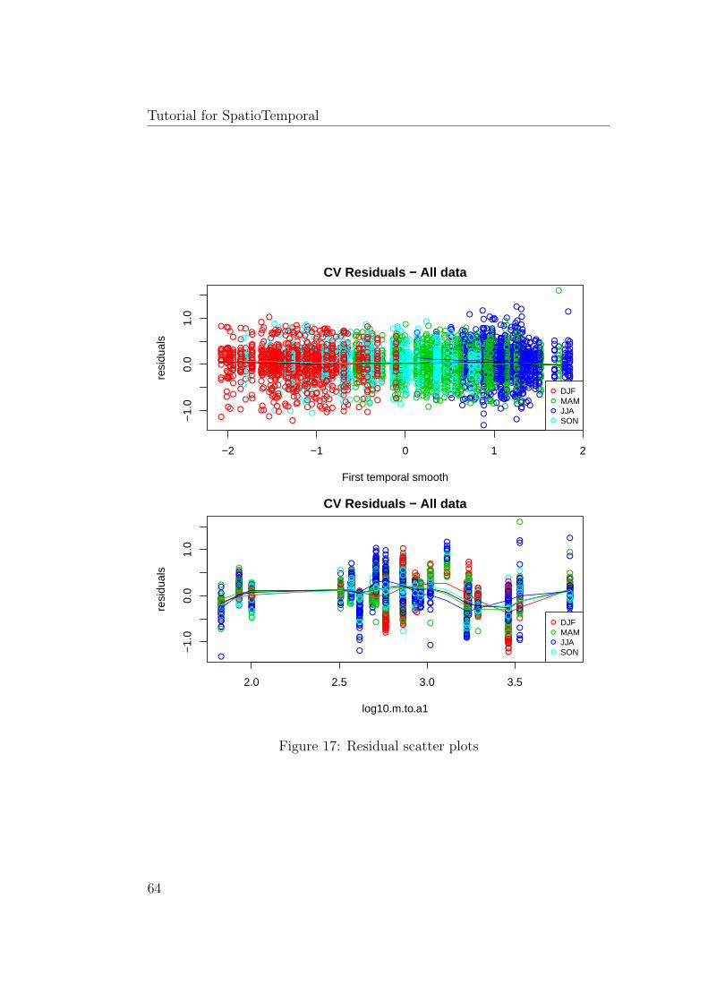
Tutorial for SpatioTemporal
●
●
●
●●●●
●
●
●
●
●
●●●
●
●
●
●
●
●
●
●
●
●
●
●
●
●● ●
●
●
●
●
●
●
●
●
●
●●
●
●●
●
●
●
●
●●
●
●
●
●●●●●●
●
●
●●
●●
●
●
●
●
●
●●
●
●
●●
●●●
●
●
●
●
●
●●
●
●
●
●
●
●
●●
●
●
●
●
●
●●
●
●
●●
●
●●
●
●
●
●
●
●
●●●
●
●●
●
●●
●
●
●
●
●
●
●
●●
●
●●
●
●
●
●
●
●●
●
●
●●
●
●●
●
●
●
●
●
●●
●
●
●
●
●
●
●
●
●●
●
●
●
●
●
●
●
●
●
●
●●●
●
●
●
●
●
●
●
●
●
●
●
●
●●●
●
●
●
●
●
●
●
●
●
●
●
●●
●
●●
●
●
●
●
●
●●
●
●●
●
●
●
●
●
●
●
●
●
●
●
●
●
●
●●
●
●
●
●
●
●
●
●
●
●
●
●
●●
●
●
●
●
●
●
●
●
●
●●●
●●
●
●
●
●
●
●
●
●
●
●
●●●
●
●●
●
●
●●
●●●
●
●●●
●
●●
●
●
●●●●
●
●
●
●●●●●
●
●
●●
●●
●
●
●
●●
●
●
●
●
●
●
●●●
●
●
●
●
●
●
●
●
●
●
●
●
●
●●
●
●
●●
●
●
●
●
●●
●●●
●
●
●
●●
●
●
●
●
●
●●●●
●
●
●
●●●
●
●
●
●
●
●
●
●● ●
●
●
●●●
●
●
●
●
●
●●
●●
●
●
●
●●●
●
●
●
●
●
●●●●
●
●
●
●●
●
●●
●
●
●●●●●
●
●
●
●●
●
●
●
●
●
●●
●●● ●
●
●●●●
●
●
●
●
●
●●
●
●●
●
●●●
●
●
●
●
●
●
●●
●
● ●
●
●●●
●
●
●
●
●
●
●●
●
●●
●
●●●
●
●●
●
●
●●●
●
●●
●
●
●●
●
●●
●
●
●●●
●
●
●●
●●
●
●
●●
●
●
●
●●
●
●●●
●
●
●
●
●●
●
●
●
●●
●
●
●●●
●
●
●
●
●
●
●
●
●●
●
●
●●
●
●
●
●
●●
●
●
●
●●
●
●
●●●●
●
●
●
●
●
●
●
●●
●
●
●
●
●
●
●
●
●●
●
●
●
●●
●
●
●
●
●
●
●
●
●
●
●
●
●
●●
●
●
●
●
●
●●
●
●●
●
●
●
●●
●
●
●
●
●●
●
●●
●
●
●●●
●
●
●
●
●●
●
●
●
●
●
●
●
●
●
●
●
●●●
●
●●
●
●
●●●
●
●
●
●●
●
●
●
●
●
●
●
●
●●●
●
●
●●●●
●
●
●
●
●●●
●
●
●
●●
●
●
●
●
●●
●
●●
●
●
●
●●
●
●
●
●
●
●
●
●●●●
●
●
●●●●
●
●
●●
●●●●
●
●
●
●●●
●
●
●
●
●
●●●●
●
●
●
●●
●
●
●
●
●
●
●
●●
●
●
●
●
●●
●
●
●
●
●
●●●●
●
●
●
●
●●
●
●
●
●
●
●●●●●
●
●
●●
●●
●
●
●
●
●●●●
●
●
●
●
●●●●
●
●
●
●
●
●
●
●
●
●●
●
●
●●●
●
●
●
●
●
●
●●
●
●●
●
●
●
●●
●
●●
●
●
●●●
●
● ●
●
●
●●●
●
●●
●
●
●
●●
●
● ●●●
●●
●
●
●
●
●
●
●
●
●
●
● ●●●
●
●
●
●
●
●
●
●
●
●
●
●
●●●
●
●
●
●
●
●
●
●
●
●
●
●
●●
●
●
●●
●
●
●
●●
●
●
●
●
●
●●●●
●
●
●
●
●
●
●
●
●
●
●
●
●●●●
●
●●
●
●
●
●
●
●
●
●
●
●●●
●
●●
●
●
●
●
●
●
●
●
●
●●●
●
●
●●
●
●●
●
●
●
●
●
●●●●
●
●
●●●●
●
●
●
●
●
●●
●
●
●
●
●
●
●
●●
●●●
●
●
●
●
●
●
●
●
●
●
●
●
●
●●
●
●●
●
●
●
●
●●
●
●
●
●
●
●
●●●●●●
●
●
●
●●●
●
●
●
●●
●
●●
●●
●
●
●
●●●
●●●
●●
●
●
●
●●
●●
●●
●
●●●●●●
●
●
●
●
●
●
●
●●
●
●
●
●
●
●
●●
●●
●
●
●
●
●
●
●
●
●
●
●
●
●
●●●
●●
●
●
●
●
●
●●●
●
●
●
●
●
●●●●●●
●
●
●
●
●
●●●
●
●
●
●
●●●●●
●
●
●
●
●
●●
●●
●
●
●
●●●
●●
●
●
●
●
●
●
●
●
●●
●
●●●●
●● ●
●
●
●
●●●●
●●
●
●
●
●●●●●
●
●
●
●
●
●●
●
●●
●
●
●●
●●●
● ●
●
●
●
●●●
●
●●
●
●
●
●●●
●
● ●●●
●
●●
●●
●
●
●
●
●
●
●●
●
●
●●●
●
●●
●
●
●●
●
●
●●●●
●
● ●
●●
●●
●
●
●
●
●
●
●
●
●
●●
●
● ●
●
●
●
●
●
●
●
●●
●
●
●
●●
●●
● ●●●
●
●●
●●
●●
●
●
●
●●
●●
●●●
●
●
●
●●
●●
●
●
●
●
●
●
●●●
●
●●
●●
●
●
●
●
●
●●●
●
●
●●
●
●
●
●●
●
●
●
●
●
●
●●
●
●
●●
●
●●
●●
●●
●
●
●
●
●●
●
●
●
●
●●
●
●
●●
●
●
●
●
●●
●
●●●
●●
●●
●●
●
●
●
●●
●
●
●
●●
●
●●
●
●
●●●●
●
●
●
●●
●●●●
●
●
●
●●●
●
●
●
●●
●
●
●●
●
●
●●
●●●
●
●
●●
●
●●
●
●
●
●
●
●
●●●
●
●
●
●●●
●
●●
●
●
●
●●●●●
●
●
●
●
●
●
●●
●
●
●
●
●●
●●●
●
●
●●
●
●
●
●
●
●
●
●●
●●●
●
●
●●●
●
●
●
●●●●●●
●
●
●
●●●●
●
●
●
●
●●●
●●
●
●●
●●●
●●
●
●●●●●●●
●
●
●
●●●
●●
●
●●●●●
●●
●
●
●
●
●●
●●
●
●●●●●
●●
●
●
●●●●
●●
●
●●●●●●
●
●
●
●
●●●
●
●
●
●●●●●●
●
●
●
●
●●
●
●●
●
●●●●●
●
●
●
●
●●●
●
●●
●
●
●
●●●
●
●
●
●
●●
●
●
●
●
●
●●●●
●
●
●
●
●
●●
●
●●
●
●●
●
●●
●
●
●
●
●●●
●
●
●
●
●
●
●●●
●
●●
●●
●●●●●
●
●
●●
●●●
●●●●●●●
●
●
●
●
●
●
●●●
●●
●
●●●●
●●
●
●
●
●●●●
●●●
●●●●●●
●
●
●
●
●
●
●●●
●
●
●
●
●
●
●
●
●
●
●●
●
●
●
●●
●
●
●
●
●
●
●●
●●●
●
●
●
●
●●
●
●●
●●
●●
●
●●●●
●●
●
●
●
●
●
●
●●
●●
●
●●●●
●
●
●
●●●
●●●●●●●●●
●
●
●
●
●
●
●●
●
●●●●●●
●
●
●
●●●
●●
●
●●●●
●●
●
●
●●
●●
●●
●
●●●
●●
●
●
●
●
●
●●
●
●
●
●●●
●
●
●
●
●●
●
●●●
●●
●●●●
●
●
●
●●
●
●●
●
●●
●
●●●
●
●
●
●
●
●
●
●
●
●
●
●
●●●
●
●
●
●
●●
●●
●
●●
●●
●
●
●
●
●●●●
●
●
●
●
●●
●
●●
●
●
●
●
●
●●
●
●
●
●●
●
●●
●
●
●
●●●●
●
●
●
●●
●
●●
●
●
●
●
●●
● ●
●
●
●●
●●
●
●
●
●
●●
●
●●
●●●
●
●●
●
●
●
●
●
●
●
●
●●●
●
●●
●
●
●●
●
●
●
●
●
●
●
●
●
●
●
●
●
●●
●
● ●●●
●●
●
●●
●
●
●
●
●●
●
●
●
●
●
●
●
●
●
●
●
●
●
●
●
●
●
●
●
●
●
●
●
●
●
●
●●
●
●
●
●
●
●
●
●
●
●●
●
●
●
●
●
●
●
●
●●
●
●
●
●●
●
●
●
●
●●
●
●●
●●●
●
●●
●
●
●
●
●●
●
●
●
●●
●
●
●●
●
●
●
●
●●
●
●
●●
●
●
●
●
●
●
●
●
●
●
●
●
●
●●
●
●
●●
●
●
●
●●
●
●
●●●
●
●
●●
●
●
●●
●
●
●
●
●●●
●
●●
●
●
●●
●●
●
●●
●
●●
●●●
●
●
●
●
●
●●
●
●
●
●●
●
●●
●
●
●●
●
●●
●
●
●
●●
●
●
●
●
●
●
●●●
●
●
●
●
●●●
●
●
●
●
●
●●●
●
●
●
●
●●●
●
●
●●
●
●
●●
●
●●
●
●
●
●
●
●
●
●
●
●
●
●
●●
●
●●
●
●
●
●
●
●
●
●
●
●
●
●
●●
●●●
●
●
●
●
●
●●
●
●
●
●●
●
●●
●
●
●
●
●
●
●
●●
●
●●
●
●●
●
●
●
●●●●
●
●
●
●●
●
●
●
●
●
●
●●
●
●
●●●
●●
●
●
●
●
●
●
●●
●
●
●●
●
●●
●
●
●
●
●
●
●●
●
●
●
●
●●●
●
●●
●
●
●
●
●
●
●
●●
●●
●
●
●●
●
●
●
●
●
●
●●
●
●●
●
●
●
●
●
●●
●
●
●●
●
●
●
●
●●
●
●
●
●
●
●
●
●
●
●
●
●
●
●
●
●
●
●
●
●
●●
●
●
●
●
●
●
●
●
●
●
●●
●
●●
●
●
●●
●
●
●
●
●
●●●
●
●
●
●
●●
●
●
●
●
●
●●●●
●
●●
●●
●
●
●
●
●
●●●●
●
●●
●●
●
●
●
●
●
●●
●
●●
●●
●
●
●
●
●●
●
●●●
●●
●●
●●
●
●
●●
●
●●
●
●●
●
●
●
●
●
●
●
●
●
●●
●
●
●●
●
●
●
●
●
●
●●
●●●●
●
●
●
●
●
●
●
●
●●●
●
●●
●●
●
●
●
●
●●
●●
●●
●
●
●
●
●
●
●
●●
●●
●●
●
●●
●
●●
●
●
●
●
●
●
●●●●
●●
●
●
●●
●
●
●
●●●●
●
●●
●
●
●
●
●
●
●
●
●
●●
●●●
●
●
●
●
●
●
●
●●●●
●
●
●
●●
●
●
●
●
●●●
●
●
●
●
●
●●
●
●
●
●
●
●●●
●
●
●
●
●●
●
●
●
●
●●
●●
●
●●●
●●
●
●
●
●
●●
●
●
●●●
●
●
●●
●
●●
●
●
●
●
●
●
●
●
●
●●●
●●
●
●●
●●●
●
●●
●
●
●
●
●
●●
●
●
●
● ●●
●●●
●
●●
●
●
●
●
●
●●
●●●
●
●●●●●●
●
●
●
●
●
●●
●
●
●
●
●●
●
●●
●
●
●
●
●●
●
●
●●
●●
●●●
●
●
●●
●
●●
●
●●
●
●
●●
●
●●
●
●●●●●●
●●
●
●●
●
●
●●
●●
●●
●
●
●●
●●
●
●
●
●
●
●
●
●
●●●●●
●
●
●
●●
●●●
●
●
●
●
●
●
●
●
●
●●
●
●
●●
●●
●●
●●
●
●
●
●
●
●
●
●
●●
●
●●
●
●
●●
●●
●
●
●
●
●
●
●
●
●
●
●
●
●
●●
●
●
●
●
●
●
●
●
●●●
●●
●
●
●●
●
●
●●
●
●
●●
●●
●
●
●●●●
●
●
●
●●
●
●●
●
●●●
●
●
●●●
●●
●
●
●
●●
●
●
●
●
●●
●●
●
●
●
●
●
●
●●
●
●
●●
●
●●
●
●
●●
●●
●
●●
●
●
●●
●
●
●●
●
●●
●
●●●●●
●●●
●●
●●
●
●●
●●●●
●
●●●●
●
●●
●
●●
●●
●
●
●
●
●
●●
●
●●●●●●●
●
●●
●●
●●
●
●●
●●
●
●●●●●●
●
●
●
●●
●
●
●
●
●●
●●●
●
●
●
●
●●
●
●
●
●
●
●
●●
●
●●●
●●
●●
●
●
●●●
●
●
●
●
●
●●●
●●
●
●●
●
●
●
●
●●
●
●●
●
●●●
●●
●●●
●●
●●
●
●
●●
●
●●
●
●
●
●
●●
●●●
●●
●
●
●
●
●●
●
●
●
●
●
●
●
●
●
●●●●●
●
●
●
●
●●
●
●
●
●
●
●
●●
●
●●●●●
●
●
●●
●●
●
●
●
●
●
●
●
●
●
●●
●●
●
● ●
●
●●●
●
●
●
●
●●
●●
●
●●●
●
●● ●
●
●●●
●
●●
●
●
●●●
●
●●●
●
●●
●
●
●
●
●●
●
●
●
●
●
●
●
●
●●
●
●
●
●●
●●●
●
●
●
●●
●
●●
●
●●
●●●
●●
●●●
●
●
●
●
●
●
●●
●
●
●●
●
●
●
●●
●●●●
●
●
●
●
●
●
●
●
●
●
●
●●
●●
●
●●●●
●
●●
●
●
●●
●
●
●●●●
●●
●
●●●
●
●
●
●
●
●●
●
●
●●●
●
●
●
●●
●
●●
●
●●
●
●
●●
●
●
●●●●●●
●●
●●●
●
●●
●
●
●●
●
●
●
●●
●
●●
●
●
●●
●
●
●
●
●
●●
●●
●
●●●
●
●●
●
●
●●
●
●●
●
●
●
●●
●
●●
●
●
●
●
●
●●
●●●●
●
●
●
●●
●
●
●
●
●
●●
●
●
●●
●
●●
●
●
●
●●
●●●
●
●
●
●
●
●●
●
●
●
●
●
●
●●●
●●●
●●
●
●
●●
●●●●
●
●
●●●
●●
●●●
●●
●●
●
●
●
●
●
●●
●
●●●●●●●●
●●
●
●
●●
●
●●
●
●
●
●●●●●●
●
●●
●●●
●
●
●●●●●
●
●
●
●
●●
●
●
●
●
●
●●●
●
●●
●
●●
●
●
●
●
●●
●
●
●
●
●
●●
●
●
●
●
●
●●
● ●
●
●
●●●
●
●
●
●
●●●●●●
●
●●
● ●
●
●
●●
●
●●
●
●●●●●
●●●
●●
● ●
●
●
●●
●
●●
●
●●
●●
●
●●●
●
●
●●
●
●
●●
●
●●
●
●●
●●
●
●●●
●●
●●
●●
●●
●
●
●
●
●
●
●
●
●●●
●●
●●
●
●
●●
●
●
●
●
●
●●●
●
●●●
●
●
● ●
●
●●
●
●
●
●
●
●
●
●●
●
●●
●●●●
●
●
●●
●
●
●
●
●
●●
●
●
●
●●
●
● ●●
●●
●
●
●
●
●
●
●
●
●
●●●●
●●
●
●
●●
●
●
●
●
●
●
●●
●
●
●
●●
●
●
●
●●
●●
●
●
●
●
●
●
●●
●●
●
●●●
●
●
●●●●
●●
●
●
●
●
●
●
●●
●
●
●●
●
●
●●
●
●
●
●
●
●
●
●
●
●●●
●
●
●●
●
●●
●●●
●
●
●
●
●
●
●
●
●
●●
●
●
●
●
●●●
●
●
●
●
●
●
●●
●
●
●
●
●
●●
●
●
●
●●●●
●
●
●
●
●
●●
●
●●●
●
●
●
●
●●●
●
●●
●
●
●
●
●
●
●●●
●
●
●●
●
●●●
●
●●
●
●
●●●
●
●●●
●
●
●●
●
●
●●
●
●
●
●
●
●
●●
●
●
●●
●
●
●●
●
●
●
●
●
●
●
●
●●●●
●●
●
●●
●●
●
●
●●
●
●
●
●
●
●●
●
●●
●
●●
●
●
●●
●●●
●
●
●
●
●
●
●
●●●
●
●●
●
●
●●●●
●
●
●
●●●
●
●
●●
●●●
●
●
●●
●
●●
●
●
●
●
●●
●
●
●
●
●
●●●●
●
●
●●
●
●
●
●
●●
●
●
●
●
●
●●●
●
●
●
●●
●
●
●
●
●●●
●
●
●
●
●●●
●●
●●●
●
●
●
●
●●
●
●
●
●
●●●●
●●
●
●●
●
●●
●
●●
●
●
●
●
●
●●
●
●●●
●●
●
●
●
●
●●
●
●
●
●
●
●
●
●
●●●
●●
●
●
●
●
●●
●
●
●
●
●●●
●
●
●●●●
●
●
●
●
●●
●
●
●
●
●
●
●
●
●●●
●
●
●
●●
●●●
●
●
●
●●
●
●
●
●●●●●
●
●
●
●
●
●●
●
●
●
●
●
●
●
●
●
●
●
●
●
●●
●
●
●
●
●
●
●
●
●
●
●
●
●
●●
●
●●●
●
●
●
●
●
●
●
●
●
●
●●
●
●
●●
●●●
●
●●●
●
●
●●●
●
●
●
●
●●
●●●
●
●●
●●
●
●
●
●●
●
●
●
●●●●
●
●
●
●
●
●
●
●
●●
●
●
●
●
●
●
●
●
●●
●
●
●●
●
●●
●
●
●
●
●
●●●
●
●●
●
●●
●
●
●
●
●
●●
●
●
●●
●
●●
●
●
●
●
●●●
●
●
−2 −1 0 1 2
−1.
00.
01.
0
CV Residuals − All data
First temporal smooth
resi
dual
s
●
●
●
●
DJFMAMJJASON
●
●
●
●● ●
●
●
●
●
●
●
●● ●
●
●
●
●
●
●
●
●
●
●
●
●
●
● ●●
●
●
●
●
●
●
●
●
●
●●
●
●●
●
●
●
●
●●
●
●
●
●●
●● ● ●
●
●
●●
●●
●
●
●
●
●
● ●
●
●
●●
●● ●
●
●
●
●
●
●●
●
●
●
●
●
●
● ●
●
●
●
●
●
●●
●
●
●●
●
●●
●
●
●
●
●
●
●●
●
●
●●
●
●●
●
●
●
●
●
●
●
● ●
●
●●
●
●
●
●
●
● ●
●
●
●●
●
●●
●
●
●
●
●
●●
●
●
●
●
●
●
●
●
●●
●
●
●
●
●
●
●
●
●
●
●● ●
●
●
●
●
●
●
●
●
●
●
●
●
●●
●
●
●
●
●
●
●
●
●
●
●
●
●●
●
●●
●
●
●
●
●
●●
●
●●
●
●
●
●
●
●
●
●
●
●
●
●
●
●
●●
●
●
●
●
●
●
●
●
●
●
●
●
●●
●
●
●
●
●
●
●
●
●
●●●
● ●
●
●
●
●
●
●
●
●
●
●
●●
●
●
●●
●
●
●●
● ●●
●
●●
●
●
●●
●
●
●● ●
●●
●
●
●●
●●●
●
●
●●
● ●
●
●
●
●●
●
●
●
●
●
●
● ● ●●
●
●
●
●
●
●
●
●
●
●
●
●
●●
●
●
●●
●
●
●
●
●●
●●
●
●
●
●
● ●
●
●
●
●
●
●● ● ●
●
●
●
●● ●
●
●
●
●
●
●
●
●●●
●
●
● ●●
●
●
●
●
●
● ●
●●
●
●
●
●●
●
●
●
●
●
●
● ●●
●
●
●
●
● ●
●
●●
●
●
●●
●● ●
●
●
●
●●
●
●
●
●
●
●●
● ●●●
●
●●
●●
●
●
●
●
●
● ●
●
●●
●
●●
●
●
●
●
●
●
●
●●
●
●●
●
●● ●
●
●
●
●
●
●
● ●
●
●●
●
●●●
●
●●
●
●
●●
●
●
●●
●
●
●●
●
●●
●
●
●●
●
●
●
● ●
●●
●
●
●●
●
●
●
●●
●
●●
●
●
●
●
●
●●
●
●
●
●●
●
●
●●
●
●
●
●
●
●
●
●
●
●●
●
●
● ●
●
●
●
●
●●
●
●
●
● ●
●
●
● ●●●
●
●
●
●
●
●
●
●●
●
●
●
●
●
●
●
●
●●
●
●
●
● ●
●
●
●
●
●
●
●
●
●
●
●
●
●
●●
●
●
●
●
●
● ●
●
●●
●
●
●
● ●
●
●
●
●
● ●
●
●●
●
●
●●●
●
●
●
●
●●
●
●
●
●
●
●
●
●
●
●
●
●● ●
●
●●
●
●
●● ●
●
●
●
●●
●
●
●
●
●
●
●
●
● ●●
●
●
●● ●
●
●
●
●
●
●●
●●
●
●
● ●
●
●
●
●
●●
●
●●
●
●
●
● ●
●
●
●
●
●
●
●
●● ●●
●
●
● ●●
●
●
●
●●
●● ●
●
●
●
●
● ●●
●
●
●
●
●
● ●● ●
●
●
●
●●
●
●
●
●
●
●
●
● ●
●
●
●
●
●●
●
●
●
●
●
●● ● ●
●
●
●
●
● ●
●
●
●
●
●
●●● ●
●●
●
● ●
● ●
●
●
●
●
●●●
●
●
●
●
●
●●● ●
●
●
●
●
●
●
●
●
●
●●
●
●
●●●
●
●
●
●
●
●
●●
●
●●
●
●
●
● ●
●
●●
●
●
●●
●
●
●●
●
●
●●
●
●
●●
●
●
●
●●
●
●●●
●
●●
●
●
●
●
●
●
●
●
●
●
●● ●●
●
●
●
●
●
●
●
●
●
●
●
●
●●
●
●
●
●
●
●
●
●
●
●
●
●
●
●●
●
●
●●
●
●
●
●●
●
●
●
●
●
●● ●●
●
●
●
●
●
●
●
●
●
●
●
●
●●●●
●
●●
●
●
●
●
●
●
●
●
●
●●●
●
●●
●
●
●
●
●
●
●
●
●
●●
●
●
●
●●
●
●●
●
●
●
●
●
●● ●●
●
●
●●
●●
●
●
●
●
●
●●
●
●
●
●
●
●
●
● ●
●●●
●
●
●
●
●
●
●
●
●
●
●
●
●
● ●
●
●●
●
●
●
●
●●
●
●
●
●
●
●
●●● ●
●●
●
●
●
● ●●
●
●
●
●●
●
●●
● ●
●
●
●
●●
●
●● ●
●●
●
●
●
●●
●●
●●
●
●●●
●● ●
●
●
●
●
●
●
●
● ●
●
●
●
●
●
●
●●
●●
●
●
●
●
●
●
●
●
●
●
●
●
●
●●
●
● ●
●
●
●
●
●
●●
●
●
●
●
●
●
● ●●
●●
●
●
●
●
●
●
●●
●
●
●
●
●
●●
● ●●
●
●
●
●
●
●●
●●
●
●
●
●●
●
● ●
●
●
●
●
●
●
●
●
●●
●
●●●●
●●●
●
●
●
●●
●●
●●
●
●
●
●●
●●
●●
●
●
●
●
●●
●
●●
●
●
●●
●●●
●●
●
●
●
●●●
●
●●
●
●
●
● ●●
●
●● ●●
●
●●
●●
●
●
●
●
●
●
●●
●
●
● ●●
●
●●
●
●
●●
●
●
●●
●●
●
●●
●●
●●
●
●
●
●
●
●
●
●
●
●●
●
●●
●
●
●
●
●
●
●
●●
●
●
●
●●
●●
●●●
●
●
●●
●●
●●
●
●
●
●●
●●
●●
●
●
●
●
●●
●●
●
●
●
●
●
●
●● ●
●
●●
● ●
●
●
●
●
●
● ●●
●
●
● ●
●
●
●
●●
●
●
●
●
●
●
●●
●
●
●●
●
●●
●●
●●
●
●
●
●
●●
●
●
●
●
●●
●
●
●●
●
●
●
●
●●
●
●●
●
●●
●●
●●
●
●
●
●●
●
●
●
●●
●
●●
●
●
●●
●●
●
●
●
●●
●●
●●
●
●
●
●●
●
●
●
●
●●
●
●
●●
●
●
●●
●●
●
●
●
●●
●
●●
●
●
●
●
●
●
●●
●
●
●
●
●● ●
●
●●
●
●
●
● ●● ●
●●
●
●
●
●
●
●●
●
●
●
●
●●
● ●●
●
●
● ●
●
●
●
●
●
●
●
●●
● ●●
●
●
● ● ●
●
●
●
●● ●●
● ●
●
●
●
●●
●●
●
●
●
●
●●●
●●
●
●●
●●
●
●●
●
●●
● ●●
● ●
●
●
●
●●
●
●●
●
●●● ●●
● ●
●
●
●
●
●●
●●
●
●●●●●
●●
●
●
●●
●●
●●
●
●●● ●●
●
●
●
●
●
● ●●
●
●
●
●●●
●●
●
●
●
●
●
●●
●
●●
●
●●●●●
●
●
●
●
●●●
●
●●
●
●
●
●● ●
●
●
●
●
● ●
●
●
●
●
●
●●●●
●
●
●
●
●
●●
●
●●
●
●●
●
●●
●
●
●
●
●● ●
●
●
●
●
●
●
● ●●
●
●●
●●
●●
●●●
●
●
●●
●●●
●● ●
●●●
●
●
●
●
●
●
●
●●●
●●
●
●●
●●
●●
●
●
●
● ●● ●
●●
●
●●
●●●
●
●
●
●
●
●
●
●●●
●
●
●
●
●
●
●
●
●
●
●●
●
●
●
●●
●
●
●
●
●
●
● ●
●●●
●
●
●
●
●●
●
●●
●●
●●
●
●●●
●
●●
●
●
●
●
●
●
●●
●●
●
●●
●●
●
●
●
● ●●
●● ●●●● ●●
●
●
●
●
●
●
●
●●
●
●● ●●
●●
●
●
●
●● ●
●●
●
●● ●
●
●●
●
●
●●
●●
●●
●
●● ●
●●
●
●
●
●
●
●●
●
●
●
●●
●
●
●
●
●
●●
●
●●●
●●
●●
●●
●
●
●
●●
●
● ●
●
●●
●
●●
●
●
●
●
●
●
●
●
●
●
●
●
●
●●●
●
●
●
●
●●
●●
●
●●
● ●
●
●
●
●
●●● ●
●
●
●
●
●●
●
●●
●
●
●
●
●
●●
●
●
●
●●
●
●●
●
●
●
●● ●
●
●
●
●
●●
●
●●
●
●
●
●
●●
●●
●
●
●●
●●
●
●
●
●
● ●
●
●●
●●
●
●
●●
●
●
●
●
●
●
●
●
●●
●
●
●●
●
●
●●
●
●
●
●
●
●
●
●
●
●
●
●
●
● ●
●
●●●
●
● ●
●
●●
●
●
●
●
● ●
●
●
●
●
●
●
●
●
●
●
●
●
●
●
●
●
●
●
●
●
●
●
●
●
●
●
●●
●
●
●
●
●
●
●
●
●
●●
●
●
●
●
●
●
●
●
●●
●
●
●
●●
●
●
●
●
● ●
●
● ●
●● ●
●
●●
●
●
●
●
● ●
●
●
●
●●
●
●
●●
●
●
●
●
●●
●
●
●●
●
●
●
●
●
●
●
●
●
●
●
●
●
●●
●
●
●●
●
●
●
● ●
●
●
●●●
●
●
●●
●
●
● ●
●
●
●
●
●● ●
●
●●
●
●
● ●
● ●
●
●●
●
● ●
●●
●
●
●
●
●
●
●●
●
●
●
●●
●
●●
●
●
● ●
●
●●
●
●
●
● ●
●
●
●
●
●
●
●● ●
●
●
●
●
●●
●
●
●
●
●
●
●● ●
●
●
●
●
●●
●
●
●
●●
●
●
● ●
●
●●
●
●
●
●
●
●
●
●
●
●
●
●
●●
●
●●
●
●
●
●
●
●
●
●
●
●
●
●
●●
●●
●
●
●
●
●
●
● ●
●
●
●
●●
●
●●
●
●
●
●
●
●
●
●●
●
●●
●
●●
●
●
●
●● ●
●●
●
●
●●
●
●
●
●
●
●
●●
●
●
●●
●
●●
●
●
●
●
●
●
●●
●
●
●●
●
●●
●
●
●
●
●
●
●●
●
●
●
●
●● ●
●
●●
●
●
●
●
●
●
●
●●
●●
●
●
● ●
●
●
●
●
●
●
●●
●
●●
●
●
●
●
●
●●
●
●
● ●
●
●
●
●
●●
●
●
●
●
●
●
●
●
●
●
●
●
●
●
●
●
●
●
●
●
● ●
●
●
●
●
●
●
●
●
●
●
●●
●
●●
●
●
●●
●
●
●
●
●
●● ●
●
●
●
●
●●
●
●
●
●
●
●● ●●
●
● ●
● ●
●
●
●
●
●
●●●
●
●
●●
● ●
●
●
●
●
●
●●
●
●●
●●
●
●
●
●
●●
●
●●●
●●
●●
●●
●
●
●●
●
●●
●
●●
●
●
●
●
●
●
●
●
●
●●
●
●
●●
●
●
●
●
●
●
● ●
●●
●●
●
●
●
●
●
●
●
●
● ●●
●
●●
● ●
●
●
●
●
●●
●●
●●
●
●
●
●
●
●
●
●●
●●
● ●
●
●●
●
● ●
●
●
●
●
●
●
● ●● ●
●●
●
●
●●
●
●
●
●●
●●
●
●●
●
●
●
●
●
●
●
●
●
●●
●●●
●
●
●
●
●
●
●
●●
●●
●
●
●
● ●
●
●
●
●
● ●●
●
●
●
●
●
● ●
●
●
●
●
●
●●
●
●
●
●
●
●●
●
●
●
●
●●
● ●
●
●●●
●●
●
●
●
●
●●
●
●
●●●
●
●
●●
●
●●
●
●
●
●
●
●
●
●
●
●●●
●●
●
● ●
●●
●
●
●●
●
●
●
●
●
●●
●
●
●
● ● ●
●● ●
●
● ●
●
●
●
●
●
●●
●●
●
●
● ●●● ●
●
●
●
●
●
●
●●
●
●
●
●
●●
●
● ●
●
●
●
●
● ●
●
●
●●
●●
●●
●
●
●
● ●
●
● ●
●
● ●
●
●
●●
●
●●
●
●●
●●● ●
●●
●
●●
●
●
●●
●●
●●
●
●
●●
● ●
●
●
●
●
●
●
●
●
●●
● ●●
●
●
●
●●
●●
●
●
●
●
●
●
●
●
●
●
● ●
●
●
●●
●●
● ●
● ●
●
●
●
●
●
●
●
●
● ●
●
●●
●
●
● ●
●●
●
●
●
●
●
●
●
●
●
●
●
●
●
● ●
●
●
●
●
●
●
●
●
●●
●
●●
●
●
●●
●
●
● ●
●
●
●●
●●
●
●
●●
●●
●
●
●
● ●
●
● ●
●
●●●
●
●
●● ●
●●
●
●
●
●●
●
●
●
●
●●
●●
●
●
●
●
●
●
●●
●
●
● ●
●
●●
●
●
●●
● ●
●
●●
●
●
●●
●
●
● ●
●
●●
●
●●●
●●
●●●
●●
●●
●
●●
● ●●●
●
●●●
●
●
●●
●
● ●
●●
●
●
●
●
●
●●
●
●●●●
● ●●
●
● ●
● ●
●●
●
●●
●●
●
●● ●●●
●
●
●
●
● ●
●
●
●
●
●●
●●●
●
●
●
●
● ●
●
●
●
●
●
●
●●
●
●●
●
● ●
●●
●
●
● ●●
●
●
●
●
●
●●●
●●
●
●●
●
●
●
●
●●
●
● ●
●
●●
●
●●
●●●
● ●
●●
●
●
● ●
●
● ●
●
●
●
●
● ●
●●●
● ●
●
●
●
●
● ●
●
●
●
●
●
●
●
●
●
●●●●
●
●
●
●
●
●●
●
●
●
●
●
●
●●
●
●●●
●●
●
●
●●
●●
●
●
●
●
●
●
●
●
●
●●
●●
●
● ●
●
●●
●
●
●
●
●
●●
●●
●
●●
●
●
●● ●
●
●●●
●
● ●
●
●
●●
●
●
●●●
●
●●
●
●
●
●
● ●
●
●
●
●
●
●
●
●
●●
●
●
●
●●
●●●
●
●
●
●●
●
● ●
●
●●
● ●●
●●
●●●
●
●
●
●
●
●
● ●
●
●
●●
●
●
●
●●
●●●
●
●
●
●
●
●
●
●
●
●
●
●
● ●
●●
●
●●● ●
●
● ●
●
●
● ●
●
●
●●
●●
●●
●
●● ●
●
●
●
●
●
● ●
●
●
●●
●
●
●
●
●●
●
● ●
●
● ●
●
●
● ●
●
●
●●●
●●
●
●●
●●●
●
●●
●
●
● ●
●
●
●
●●
●
●●
●
●
●●
●
●
●
●
●
●●
●●
●
●●●
●
●●
●
●
●●
●
● ●
●
●
●
●●
●
●●
●
●
●
●
●
●●
● ●● ●
●
●
●
● ●
●
●
●
●
●
● ●
●
●
● ●
●
●●
●
●
●
● ●
●●
●
●
●
●
●
●
● ●
●
●
●
●
●
●
●● ●
●●●
●●
●
●
●●
●●
●●
●
●
●● ●
● ●
●●
●
●●
● ●
●
●
●
●
●
●●
●
●●
●● ●
●●●
●●
●
●
●●
●
●●
●
●
●
●● ●
●●
●
●
●●
●●
●
●
●
●●
●●●
●
●
●
●
● ●
●
●
●
●
●
● ●●
●
●●
●
● ●
●
●
●
●
● ●
●
●
●
●
●
●●
●
●
●
●
●
● ●
● ●
●
●
● ●●
●
●
●
●
● ●●●
●●
●
●●
● ●
●
●
●●
●
●●
●
●● ●●
●
●●●
●●
● ●
●
●
● ●
●
● ●
●
●●
●●
●
●●●
●
●
●●
●
●
●●
●
● ●
●
●●
●●
●
●●●
● ●
●●
●●
●●
●
●
●
●
●
●
●
●
●●●
●●
●●
●
●
● ●
●
●
●
●
●
● ●●
●
●●●
●
●
● ●
●
●●
●
●
●
●
●
●
●
●●
●
●●
●●
●●
●
●
●●
●
●
●
●
●
●●
●
●
●
●●
●
● ● ●
●●
●
●
●
●
●
●
●
●
●
●●
● ●
●●
●
●
●●
●
●
●
●
●
●
● ●
●
●
●
●●
●
●
●
● ●
●●
●
●
●
●
●
●
●●
●●
●
●●
●
●
●
● ●●●
● ●
●
●
●
●
●
●
●●
●
●
●●
●
●
● ●
●
●
●
●
●
●
●
●
●
●●
●
●
●
●●
●
● ●
●●●
●
●
●
●
●
●
●
●
●
●●
●
●
●
●
● ●●
●
●
●
●
●
●
●●
●
●
●
●
●
●●
●
●
●
●●
●●
●
●
●
●
●
●●
●
●● ●
●
●
●
●
●● ●
●
● ●
●
●
●
●
●
●
●●●
●
●
●●
●
●● ●
●
●●
●
●
● ●●
●
●●●
●
●
●●
●
●
●●
●
●
●
●
●
●
●●
●
●
●●
●
●
● ●
●
●
●
●
●
●
●
●
●●●
●
●●
●
●●
●●
●
●
● ●
●
●
●
●
●
●●
●
●●
●
● ●
●
●
●●
● ● ●
●
●
●
●
●
●
●
●●
●
●
● ●
●
●
●● ●
●
●
●
●
●● ●
●
●
●●
●●
●
●
●
●●
●
● ●
●
●
●
●
●●
●
●
●
●
●
●● ●●
●
●
● ●
●
●
●
●
● ●
●
●
●
●
●
●●
●
●
●
●
● ●
●
●
●
●
●●
●
●
●
●
●
●●●
●●
●● ●
●
●
●
●
●●
●
●
●
●
●●
●●
●●
●
● ●
●
●●
●
● ●
●
●
●
●
●
●●
●
●●
●
●●
●
●
●
●
●●
●
●
●
●
●
●
●
●
●●●
●●
●
●
●
●
●●
●
●
●
●
●●
●
●
●
●●● ●
●
●
●
●
● ●
●
●
●
●
●
●
●
●
●●●
●
●
●
● ●
●●
●
●
●
●
●●
●
●
●
●●● ● ●
●
●
●
●
●
●●
●
●
●
●
●
●
●
●
●
●
●
●
●
●●
●
●
●
●
●
●
●
●
●
●
●
●
●
●●
●
●●●
●
●
●
●
●
●
●
●
●
●
●●
●
●
●●
●●
●
●
●●
●
●
●
●●
●
●
●
●
●
●●
●●
●
●
● ●
●●
●
●
●
●●
●
●
●
●●●
●
●
●
●
●
●
●
●
●
●●
●
●
●
●
●
●
●
●
● ●
●
●
●●
●
●●
●
●
●
●
●
● ●●
●
●●
●
●●
●
●
●
●
●
● ●
●
●
●●
●
●●
●
●
●
●
●●
●
●
●
2.0 2.5 3.0 3.5
−1.
00.
01.
0
CV Residuals − All data
log10.m.to.a1
resi
dual
s
●
●
●
●
DJFMAMJJASON
Figure 17: Residual scatter plots
64
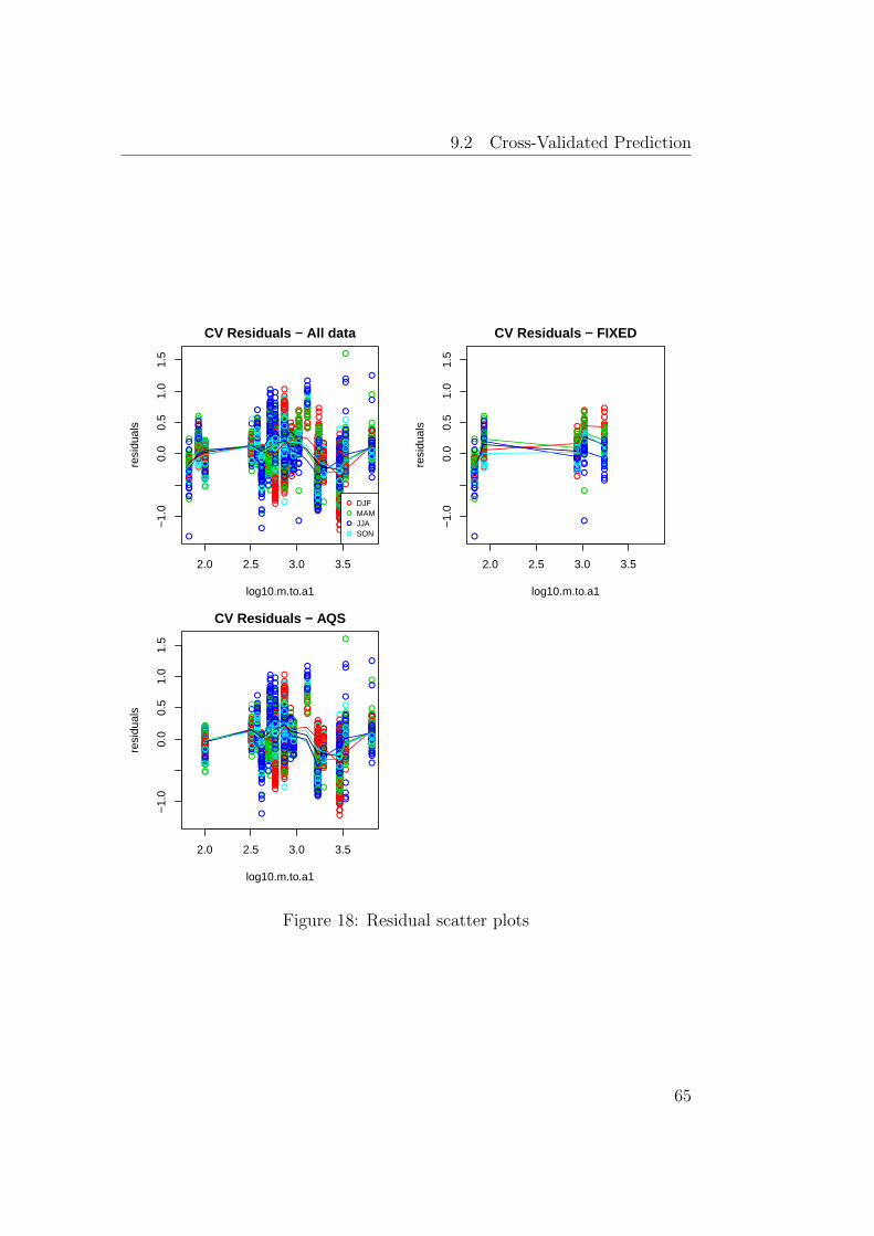
9.2 Cross-Validated Prediction
●
●
●
●
● ●●
●
●
●
●
●
●
● ●●
●
●
●
●
●
●
●
●
●
●
●
●
● ●●
●
●
●
●
●
●
●
●
●
●●
●
●●
●
●
●
●
●
●
●
●
●
●●●
●
●●
●
●
●●
●
●
●
●
●
●
●
●●
●
●
●●
●
● ●
●
●
●
●
●
●●
●●
●
●
●
●
● ●
●
●
●
●
●
●●
●
●
●●
●
●●
●
●
●
●
●
●
●
●●
●
●●
●
●
●
●
●
●
●
●
●
●
●●
●
●●
●
●
●
●
●
●●
●
●
● ●
●
●●
●
●
●
●
●
●●
●
●
●
●
●
●
●
●
●●
●
●
●
●
●
●
●
●
●
●
●
●●
●
●
●
●
●
●
●
●
●
●
●
●
●
●●
●
●
●
●
●
●
●
●
●
●
●
●●
●
●●
●
●
●
●
●
●
●
●
●●
●
●
●
●
●
●
●
●
●
●
●
●
●
●
●
●
●
●
●
●
●
●
●
●
●
●
●
●
●●
●
●
●
●
●
●
●
●
●
●●
●
●●
●
●
●
●
●
●
●
●
●
●
●●
●
●
●●
●
●
●●
●●
●
●
●●
●
●
●●
●
●
●
●●
●
●
●
●
●●
●●
●
●
●
●
●
●●
●
●
●
●
●
●
●
●
●
●
●
●● ●
●
●
●
●
●
●
●
●
●
●
●
●
●
●●
●
●
●●
●
●
●
●
●
●
●
●
●
●
●
●
● ●
●
●
●
●
●
●
● ● ●●
●
●
●● ●
●
●
●
●
●
●
●
●●●
●
●
●●
●
●
●
●
●
●
●
●
●●
●
●
●
●●
●
●
●
●
●
●
● ●
●
●
●
●
●
●●
●
●●
●
●
●●
●
●●
●
●
●
●●
●
●
●
●
●
●●
●
●
●●
●
●●
●
●
●
●
●
●
●
●●
●
●
●
●
●●
●
●
●
●
●
●
●
● ●
●
●●
●
●
● ●
●
●
●
●
●
●
●●
●
●●
●
●●
●
●
●
●
●
●
●
●
●
●
●●
●
●
●●
●
●●
●
●
●
●
●
●
●
● ●
●●
●
●
●
●
●
●
●
● ●
●
●
●
●
●
●
●
●
●●
●
●
●
●
●
●
●
●●
●
●
●
●
●
●
●
●
●
●
●
●
●
● ●
●
●
●
●
●●
●
●
●
●
●
●
●
● ●●
●
●
●
●
●
●
●
●
●
●
●
●
●
●
●
●
●
●
●●
●
●
●
●●
●
●
●
●
●
●
●
●
●
●
●
●
●
● ●
●
●
●
●
●
● ●
●
●●
●
●
●
●●
●
●
●
●
●●
●
●●
●
●
●●
●
●
●
●
●
●●
●
●
●
●
●
●
●
●
●
●
●
●
●●
●
●●
●
●
●
●●
●
●
●
●●
●
●
●
●
●
●
●
●
●
●●
●
●
●● ●
●
●
●
●
●
●
●
●●
●
●
● ●
●
●
●
●
●
●
●
● ●●
●
●
●●
●
●
●
●
●
●
●
●
●●●
●
●
●●
●●
●
●
●●
●●
●
●
●
●
●
● ●
●
●
●
●
●
●
● ●
● ●
●
●
●
●●
●
●
●
●
●
●
●
●●
●
●
●
●
●●
●
●
●
●
●
●●
●●
●
●
●
●
● ●
●
●
●
●
●
●●
● ●●
●
●
●●
● ●
●
●
●
●
●
●●●
●
●
●
●
●●
● ●
●
●
●
●
●
●
●
●
●
●●
●
●
●●●
●
●
●
●
●
●
● ●
●
●●
●
●
●
● ●
●
●●
●
●
●
●
●
●
●●
●
●
●●
●
●
●●
●
●
●
●●
●
●●
●●
●●
●
●
●
●
●
●
●
●
●
●
●● ●
●
●
●
●
●
●
●
●
●
●
●
●
●
●●
●
●
●
●
●
●
●
●
●
●
●
●
●
●●
●
●
●●
●
●
●
●●
●
●
●
●
●
●● ●
●
●
●
●
●
●
●
●
●
●
●
●
●
●●
●●
●
●
●
●
●
●
●
●
●
●
●
●
●●●
●
●●
●
●
●
●
●
●
●
●
●
●●
●
●
●
●
●
●
●●
●
●
●
●
●
●
● ●●
●
●
●●
●
●
●
●
●
●
●
●
●
●
●
●
●
●
●
●
●●
●●
●
●
●
●
●
●
●
●
●
●
●
●
●
●
● ●
●
●●
●
●
●
●
●●
●
●
●
●
●
●
●●● ●
●●
●
●
●
●●
●
●
●
●
●●
●
●●
● ●
●
●
●
●
●
●
●● ●
●●
●
●
●
●
●
●●
●●
●
●●
●
●● ●
●
●
●
●
●
●
●
●●
●
●
●
●
●
●
●●
●●
●
●
●
●
●
●
●
●
●
●
●
●
●
●
●●
● ●
●
●
●
●
●
●
●●
●
●
●
●
●
●●
●●
●
●
●
●
●
●
●
●●
●
●
●
●
●
● ●● ●●
●
●
●
●
●
●●
●●
●
●
●
●
●●
● ●
●
●
●
●
●
●
●
●
●●
●
●●
●●
●
●●
●
●
●
●●
●●
●●
●
●
●
● ●●●
●●
●
●
●
●
●●
●
●●
●
●
●●
●●
●
●●
●
●
●
●●
●
●
●●
●
●
●
● ●●
●
●● ●●
●
●●
●●
●
●
●
●
●
●
●●
●
●
●●
●
●
●●
●
●
●●
●
●
●
●
●●
●
●●
●
●
●
●
●
●
●
●
●
●
●
●
●●
●
●
●●
●
●
●
●
●
●
●
●●
●
●
●
●
●●
●
●●
●●
●
●●
●
●
●
●
●
●
●
●
●
●
●
●●
●
●
●
●
●
●
●
●
●
●
●
●
●
●
●● ●
●
●●
● ●
●
●
●
●
●
●
●●
●
●
● ●
●
●
●
●●
●
●
●
●
●
●
●●
●
●
●
●
●
●
●
●●
●●
●
●
●
●
●●
●
●
●
●
●●
●
●
●●
●
●
●
●
●●
●
●
●●
●
●
●●
●●
●
●
●
●
●
●
●
●
●●
●
●●
●
●
●
●
●●
●
●
●
●●
●●
●●
●
●
●
●●
●
●
●
●
●●
●
●
●●
●
●
●●
●●●
●
●
●●
●
●●
●
●
●
●
●
●●●
●
●
●
●
●●
●
●
●
●
●
●
●
●●● ●
●●
●
●
●
●
●
●
●
●
●
●
●
●●
●●
●
●
●
● ●
●
●
●
●
●
●
●
●●
● ●●
●
●
●● ●
●
●
●
●●
●●
● ●
●
●
●
●
●●
●
●
●
●
●
●
●●
●●
●
●
●
●●
●
●
●
●
●●
● ●●●
●
●
●
●
●
●●
●
●
●
●●
●●●
●●
●
●
●
●
●
●
●
●
●
●●
●
●●
●●
●
●
●
●●
●
●
●
●
●●●
●●●
●
●
●
●
● ●●
●
●
●
●●●
●●●
●
●
●
●
●
●
●
●●
●
●●●●●
●
●
●
●
●●●
●
●●
●
●
●
●● ●
●
●
●
●
● ●
●
●
●
●
●
●●
●●
●
●
●
●
●
●●
●
●●
●
●
●
●
●●
●
●
●
●
●● ●
●
●
●
●
●
●
●
●●
●
●●
●●
●
●
●
●●
●
●
●●
●●
●
●● ●
●●●
●
●
●
●
●
●
●
●●
●
●●
●
●●
●●
●●
●
●
●
●
●●
●
●●
●
●●
●
●●
●
●
●
●
●
●
●
●●●
●
●
●
●
●
●
●
●
●
●
●●
●
●
●
●
●
●
●
●
●
●
●
●●
●●
●
●
●
●
●
●●
●
●●
●
●
●
●
●
●●
●
●
●●
●
●
●
●
●
●
●
●
●●
●
●
●●●
●
●
●
● ●●
●● ●●●
● ●●
●
●
●
●
●
●
●
●●
●
●● ●
●●
●
●
●
●
●●
●
●●
●
●● ●
●
●●
●
●
●
●
●●
●
●
●
●● ●
●●
●
●
●
●
●
●●
●
●
●
●
●●
●
●
●
●
●
●
●
●
●●
●
●
●●
●
●
●
●
●
●
●
●
● ●
●
●●
●
●●
●
●
●
●
●
●
●
●
●
●
●
●
●
●
●●
●
●
●
●
●●
●●
●
●
●
● ●
●
●
●
●
●●● ●
●
●
●
●
●●
●
●
●
●
●
●
●
●
●●
●
●
●
●
●
●
●
●
●
●
●
●●
●●
●
●
●
●●
●
●●
●
●
●
●
●
●
●●
●
●
●●
●●
●
●
●
●
● ●
●
●●
●
●●
●
●●
●
●
●
●
●
●
●
●
●●
●
●
●●
●
●
●●
●
●
●
●
●
●
●
●
●
●
●
●
●
●●
●
●●●
●
● ●
●
●●
●
●
●
●
● ●
●
●
●
●
●
●
●
●
●
●
●
●
●
●
●
●
●
●
●
●
●
●
●
●
●
●
●
●
●
●
●
●
●
●
●
●
●
●
●
●
●
●
●
●
●
●
●
●●
●
●
●
●●
●
●
●
●
● ●
●
● ●
●●
●
●
●
●
●
●
●
●
● ●
●
●
●
●●
●
●
●●
●
●
●
●
●
●
●
●
●●
●
●
●
●
●
●
●
●
●
●
●
●
●
●●
●
●
●●
●
●
●
● ●
●
●
●●
●
●
●
●●
●
●
● ●
●
●
●
●
●● ●
●
●●
●
●
●●
● ●
●
●
●
●
● ●
●●
●
●
●
●
●
●
●●
●
●
●
●●
●
●●
●
●
● ●
●
●
●
●
●
●
● ●
●
●
●
●
●
●
●
● ●
●
●
●
●
●●
●
●
●
●
●
●
●●●
●
●
●
●
●
●●
●
●
●●
●
●
● ●
●
●
●
●
●
●
●
●
●
●
●
●
●
●
●
●
●
●
●●
●
●
●
●
●
●
●
●
●
●
●
●
●●
●
●●
●
●
●
●
●
● ●
●
●
●
●●
●
●
●
●
●
●
●
●
●
●
●●
●
●
●
●
●●
●
●
●
●
● ●
●
●
●
●
●
●
●
●
●
●
●
●
●
●
●
●
●
●
●
●●
●
●
●
●
●
●
●
●
●
●
●
●
●
●●
●
●
●
●
●
●
●●
●
●
●
●
●●
●
●
●●
●
●
●
●
●
●
●
●
●
●●
●
●
● ●
●
●
●
●
●
●
●●
●
●●
●
●
●
●
●
●
●
●
●
● ●
●
●
●
●
●
●
●
●
●
●
●
●
●
●
●
●
●
●
●
●
●
●
●
●
●
●
● ●
●
●
●
●
●
●
●
●
●
●
●●
●
●●
●
●
●●
●
●
●
●
●
●●●
●
●
●
●
●●
●
●
●
●
●
●● ●●
●
● ●
● ●
●
●
●
●
●
●●
●●
●
●●
● ●
●
●
●
●
●
●●
●
●●
●●
●
●
●
●
●●
●
●●
●
●●
●
●
●
●
●
●
●●
●
●●
●
●●
●
●
●
●
●
●
●
●
●
●●
●
●
●●
●
●
●
●
●
●
● ●
●●
●●
●
●
●
●
●
●
●
●
● ●
●●
●●
● ●
●
●
●
●
●●
●
●
●
●
●
●
●
●
●
●
●
●
●
●
●
●●
●
●
●
●
● ●
●
●
●
●
●
●
● ●● ●
●●
●
●
●●
●
●
●
●●
●●
●
●●
●
●
●
●
●
●
●
●
●
●●
●●●
●
●
●
●
●
●
●
●●
●●
●
●
●
● ●
●
●
●
●
● ●●
●
●
●
●
●
● ●
●
●
●
●
●
●●
●
●
●
●
●
●●
●
●
●
●
●
●
● ●
●
●
●●
●●
●
●
●
●
●●
●
●
●●●
●
●
●●
●
●●
●
●
●
●
●
●
●
●
●
●●
●
●
●
●
● ●
●●
●
●
●
●
●
●
●
●
●
●●
●
●
●
● ● ●
●● ●
●
●●
●
●
●
●
●
●●
●●
●
●
● ●●● ●
●
●
●
●
●
●
●●
●
●
●
●
●
●
●
●●
●
●
●
●
● ●
●
●
●●
●●
●●
●
●
●
● ●
●
● ●
●
●●
●
●
●●
●
●●
●
●●
●●
● ●
●●
●
●●
●
●
●●
●●
●●
●
●
●●
●●
●
●
●
●
●
●
●
●
●●
●●
●
●
●
●
●●
●
●●
●
●
●
●
●
●
●
●
●
● ●
●
●
●
●
●●
● ●
● ●
●
●
●
●
●
●
●
●
●●
●
●
●
●
●
● ●
●
●
●
●
●
●
●
●
●
●
●
●
●
●
●
● ●
●
●
●
●
●
●
●
●
●
●●
●●
●
●
●●
●
●
●●
●
●
●●
●●
●
●
●●
●●
●
●
●
● ●
●
●●
●
●●●
●
●
●● ●
●●
●
●
●
●●
●
●
●
●
●
●
●●
●
●
●
●
●
●
●●
●
●
● ●
●
●
●
●
●
●●
● ●
●
●●
●
●
●●
●
●
● ●
●
●
●
●
●●
●●
●
●●●
●
●
●●
●
●●
● ●●●
●
●●
●●
●
●
●
●
● ●
●
●
●
●
●
●
●
●●
●
●●●
●●
●●
●
● ●
● ●
●
●
●
●
●
●
●
●
●● ●●●
●
●
●
●
● ●
●
●
●
●
●●
●●●
●
●
●
●
●●
●
●
●
●
●
●
●
●
●
●
●●
● ●
●●
●
●
● ●●
●
●
●
●
●
●●●
●●
●
●●
●
●
●
●
●
●
●
● ●
●
●
●●
●
●
●●●
● ●
●●
●
●
● ●
●
● ●
●
●
●
●
●●
●●●
● ●
●
●
●
●
●●
●
●
●
●
●
●
●
●
●
●●●
●●
●
●
●
●
●
●
●
●
●
●
●
●
●
●
●
●●●
●●
●
●
●●
●●
●
●
●
●
●
●
●
●
●
●●
●●
●
● ●
●
●
●●
●
●
●
●
●●
●●
●
●
●●
●
●
● ●
●
●●●
●
●●
●
●
●
●
●
●
●●
●
●
●
●
●
●
●
●
● ●
●
●
●
●
●
●
●
●
●
●
●
●
●
●●
●●●
●
●
●
●●
●
● ●
●
●●
● ●
●
●●
●
●●
●
●
●
●
●
●
●●
●
●
●●
●
●
●
●●
●●●
●
●
●
●
●
●
●
●
●
●
●
●
●●
●●
●
●●● ●
●
● ●
●
●
● ●
●
●
●●
●●
●●
●
●
●●
●
●
●
●
●
● ●
●
●
●
●●
●
●
●
●●
●
●●
●
● ●
●
●
● ●
●
●
●●●
●●
●
●●
●●●
●
●●
●
●
● ●
●
●
●
●●
●
●●
●
●
●●
●
●
●
●
●
●
●
●
●
●
●●●
●
●●
●
●
●●
●
●●
●
●
●
●●
●
●●
●
●
●
●
●
●
●
● ●● ●
●
●
●
● ●
●
●
●
●
●
●●
●
●
● ●
●
●●
●
●
●
● ●
●●
●
●
●
●
●
●
● ●
●
●
●
●
●
●
●●
●
●●●
●●
●
●
●●
●●
●●
●
●
●
●●
● ●
●●
●
●
●
● ●
●
●
●
●
●
●
●
●
●●
●● ●
●●●
●●
●
●
●●
●
●
●
●
●
●
●
● ●●
●
●
●
●●
●●
●
●
●
●●
●●●
●
●
●
●
● ●
●
●
●
●
●
● ●●
●
●●
●
● ●
●
●
●
●
● ●
●
●
●
●
●
●●
●
●
●
●
●
●●
● ●
●
●
● ●
●
●
●
●
●
● ●●
●
●●
●
●●
●●
●
●
●
●
●
●
●
●
●● ●
●
●
●●
●
●●
● ●
●
●
● ●
●
● ●
●
●●
●●
●
●●●
●
●
●●
●
●
●●
●
●●
●
●●
●●
●
●●●
● ●
●●
●
●
●●
●
●
●
●
●
●
●
●
●●●
●●
●
●
●
●
● ●
●
●
●
●
●
● ●
●
●
●●
●
●
●
● ●
●
●●
●
●
●
●
●
●
●
●●
●
●●
●
●
●●
●
●
●
●
●
●
●
●
●
●●
●
●
●
●
●
●
● ● ●
●●
●
●
●
●
●
●
●
●
●
●●
●●
●●
●
●
●●
●
●
●
●
●
●
● ●
●
●
●
●●
●
●
●
● ●
●
●
●
●
●
●
●
●
●
●
●●
●
●●
●
●
●
● ●●
●
● ●
●
●
●
●
●
●
●
●
●
●
●●
●
●
● ●
●
●
●
●
●
●
●
●
●
●
●●
●
●
●
●
●
● ●
●●
●
●
●
●
●
●
●
●
●
●
●●
●
●
●
●
● ●●
●
●
●
●
●
●
●
●
●
●
●
●
●
●
●
●
●
●
●●
●●
●
●
●
●
●
●●
●
●● ●
●
●
●
●
●● ●
●
●●
●
●
●
●
●
●
●●●
●
●
●
●
●
●
● ●
●
●
●
●
●
● ●
●
●
●●
●
●
●
●
●
●
●
●●
●
●
●
●
●
●
●●
●
●
●●
●
●
● ●
●
●
●
●
●
●
●
●
●
●●
●
●●
●
●
●
●
●
●
●
● ●
●
●
●
●
●
●●
●
●●
●
●●
●
●
●●
● ● ●
●
●
●
●
●
●
●
●●
●
●
● ●
●
●
●● ●●
●
●
●
●● ●
●
●
●●
●
●●
●
●
●●
●
● ●
●
●
●
●
●●
●
●
●
●
●
●● ●
●
●
●
●●
●
●
●
●
●●
●
●
●
●
●
●
●
●
●
●
●
● ●
●
●
●
●
●●
●
●
●
●
●
●●
●
●●
●● ●
●
●
●
●
●●
●
●
●
●
●●
●●
●●
●
● ●
●
●●
●
● ●
●
●
●
●
●
●
●
●
●
●●
●
●
●
●
●
●
●●
●
●
●
●
●
●
●
●
●●
●
●
●
●
●
●
●
●●
●
●
●
●
●●
●
●
●
●●●
●
●
●
●
●
●●
●
●
●
●
●
●
●
●
●
●●
●
●
●
● ●
●
●●
●
●
●
●●
●
●
●
●●●
● ●
●
●
●
●
●
●●
●
●
●
●
●
●
●
●
●
●
●
●
●
●●
●
●
●
●
●
●
●
●
●
●
●
●
●
●●
●
●
●●
●
●
●
●
●
●
●
●
●
●
●●
●
●
●●
●●
●
●
●
●●
●
●
●●
●
●
●
●
●
●●
●
●
●
●
● ●
●●
●
●
●
●
●
●
●
●
●●●
●
●
●
●
●
●
●
●
●
●●
●
●
●
●
●
●
●
●
●●
●
●
●●
●
●●
●
●
●
●
●
● ●●
●
●
●
●
●
●
●
●
●
●
●
● ●
●
●
●●
●
●●
●
●
●
●
●●
●
●
●
2.0 2.5 3.0 3.5
−1.
00.
00.
51.
01.
5
CV Residuals − All data
log10.m.to.a1
resi
dual
s
●
●
●
●
DJFMAMJJASON
●
●
●
●
● ●●
●
●
●
●
●
●
● ●●
●
●
●
●
●
●
●
●
●
●
●
●
● ●●
●
●
●
●
●
●
●
●
●
●●
●
●●
●
●
●
●
●
●
●
●
●
●●●
●
●●
●
●
●●
●
●
●
●
●
●
●
●●
●
●
●●
●
● ●
●
●
●
●
●
●●
●●
●
●
●
●
● ●
●
●
●
●
●
●●
●
●
●●
●
●●
●
●
●
●
●
●
●
●●
●
●●
●
●
●
●
●
●
●
●
●
●
●●
●
●●
●
●
●
●
●
●●
●
●
● ●
●
●●
●
●
●
●
●
●●
●
●
●
●
●
●
●
●
●●
●
●
●
●
●
●
●
●
●
●
●
●●
●
●
●
●
●
●
●
●
●
●
●
●
●
●●
●
●
●
●
●
●
●
●
●
●
●
●●
●
●●
●
●
●
●
●
●
●
●
●●
●
●
●
●
●
●
●
●
●
●
●
●
●
●
●
●
●
●
●
●
●
●
●
●
●
●
●
●
●●
●
●
●
●
●
●
●
●
●
●●
●
●●
●
●
●
●
●
●
●
●
●
●
●●
●
●
●●
●
●
●●
●●
●
●
●●
●
●
●●
●
●
●
●●
●
●
●
●
●●
●●
●
●
●
●
●
●●
●
●
●
●
●
●
●
●
●
●
●
●● ●
●
●
●
●
●
●
●
●
●
●
●
●
●
●●
●
●
●●
●
●
●
●
●
●
●
●
●
●
●
●
● ●
●
●
●
●
●
●
● ● ●●
●
●
●● ●
●
●
●
●
●
●
●
●●●
●
●
●●
●
●
●
●
●
●
●
●
●●
●
●
●
●●
●
●
●
●
●
●
● ●
●
●
●
●
●
●●
●
●●
●
●
●●
●
●●
●
●
●
●●
●
●
●
●
●
●●
●
●
●●
●
●●
●
●
●
●
●
●
●
●●
●
●
●
●
●●
●
●
●
●
●
●
●
● ●
●
●●
●
●
● ●
●
●
●
●
●
●
●●
●
●●
●
●●
●
●
●
●
●
●
●
●
●
●
●●
●
●
●●
●
●●
●
●
●
●
●
●
●
● ●
●●
●
●
●
●
●
●
●
● ●
●
●
●
●
●
●
●
●
●●
●
●
●
●
●
●
●
●●
●
●
●
●
●
●
●
●
●
●
●
●
●
● ●
●
●
●
●
●●
●
●
●
●
●
●
●
● ●●
●
●
●
●
●
●
●
●
●
●
●
●
●
●
●
●
●
●
●●
●
●
●
●●
●
●
●
●
●
●
●
●
●
●
●
●
●
● ●
●
●
●
●
●
● ●
●
●●
●
●
●
●●
●
●
●
●
●●
●
●●
●
●
●●
●
●
●
●
●
●●
●
●
●
●
●
●
●
●
●
●
●
●
●●
●
●●
●
●
●
●●
●
●
●
●●
●
●
●
●
●
●
●
●
●
●●
●
●
●● ●
●
●
●
●
●
●
●
●●
●
●
● ●
●
●
●
●
●
●
●
● ●●
●
●
●●
●
●
●
●
●
●
●
●
●●●
●
●
●●
●●
●
●
●●
●●
●
●
●
●
●
● ●
●
●
●
●
●
●
● ●
● ●
●
●
●
●●
●
●
●
●
●
●
●
●●
●
●
●
●
●●
●
●
●
●
●
●●
●●
●
●
●
●
● ●
●
●
●
●
●
●●
● ●●
●
●
●●
● ●
●
●
●
●
●
●●●
●
●
●
●
●●
● ●
●
●
●
●
●
●
●
●
●
●●
●
●
●●●
●
●
●
●
●
●
● ●
●
●●
●
●
●
● ●
●
●●
●
●
●
●
●
●
●●
●
●
●●
●
●
●●
●
●
●
●●
●
●●
●●
●●
●
●
●
●
●
●
●
●
●
●
●● ●
●
●
●
●
●
●
●
●
●
●
●
●
●
●●
●
●
●
●
●
●
●
●
●
●
●
●
●
●●
●
●
●●
●
●
●
●●
●
●
●
●
●
●● ●
●
●
●
●
●
●
●
●
●
●
●
●
●
●●
●●
●
●
●
●
●
●
●
●
●
●
●
●
●●●
●
●●
●
●
●
●
●
●
●
●
●
●●
●
●
●
●
●
●
●●
●
●
●
●
●
●
● ●●
●
●
●●
●
●
●
●
●
●
●
●
●
●
●
●
●
●
●
●
●●
●●
●
●
●
●
●
●
●
●
●
●
●
●
●
●
● ●
●
●●
●
●
●
●
●●
●
●
●
●
●
●
●●● ●
●●
●
●
●
●●
●
●
●
●
●●
●
●●
● ●
●
●
●
●
●
●
●● ●
●●
●
●
●
●
●
●●
●●
●
●●
●
●● ●
●
●
●
●
●
●
●
●●
●
●
●
●
●
●
●●
●●
●
●
●
●
●
●
●
●
●
●
●
●
●
●
●●
● ●
●
●
●
●
●
●
●●
●
●
●
●
●
●●
●●
●
●
●
●
●
●
●
●●
●
●
●
●
●
● ●● ●●
●
●
●
●
●
●●
●●
●
●
●
●
●●
● ●
●
●
●
●
●
●
●
●
●●
●
●●
●●
●
●●
●
●
●
●●
●●
●●
●
●
●
● ●●●
●●
●
●
●
●
●●
●
●●
●
●
●●
●●
●
●●
●
●
●
●●
●
●
●●
●
●
●
● ●●
●
●● ●●
●
●●
●●
●
●
●
●
●
●
●●
●
●
●●
●
●
●●
●
●
●●
●
●
●
●
●●
●
●●
●
●
●
●
●
●
●
●
●
●
●
●
●●
●
●
●●
●
●
●
●
●
●
●
●●
●
●
●
●
●●
●
●●
●●
●
●●
●
●
●
●
●
●
●
●
●
●
●
●●
●
●
●
●
●
●
●
●
●
●
●
●
●
●
●● ●
●
●●
● ●
●
●
●
●
●
●
●●
●
●
● ●
●
●
●
●●
●
●
●
●
●
●
●●
●
●
●
●
●
●
●
●●
●●
●
●
●
●
●●
●
●
●
●
●●
●
●
●●
●
●
●
●
●●
●
●
●●
●
●
●●
●●
●
●
●
●
●
●
●
●
●●
●
●●
●
●
●
●
●●
●
●
●
●●
●●
●●
●
●
●
●●
●
●
●
●
●●
●
●
●●
●
●
●●
●●●
●
●
●●
●
●●
●
●
●
●
●
●●●
●
●
●
●
●●
●
●
●
●
●
●
●
●●● ●
●●
●
●
●
●
●
●
●
●
●
●
●
●●
●●
●
●
●
● ●
●
●
●
●
●
●
●
●●
● ●●
●
●
●● ●
●
●
●
●●
●●
● ●
●
●
●
●
●●
●
●
●
●
●
●
●●
●●
●
●
●
●●
●
●
●
●
●●
● ●●●
●
●
●
●
●
●●
●
●
●
●●
●●●
●●
●
●
●
●
●
●
●
●
●
●●
●
●●
●●
●
●
●
●●
●
●
●
●
●●●
●●●
●
●
●
●
● ●●
●
●
●
●●●
●●●
●
●
●
●
●
●
●
●●
●
●●●●●
●
●
●
●
●●●
●
●●
●
●
●
●● ●
●
●
●
●
● ●
●
●
●
●
●
●●
●●
●
●
●
●
●
●●
●
●●
●
●
●
●
●●
●
●
●
●
●● ●
●
●
●
●
●
●
●
●●
●
●●
●●
●
●
●
●●
●
●
●●
●●
●
●● ●
●●●
●
●
●
●
●
●
●
●●
●
●●
●
●●
●●
●●
●
●
●
●
●●
●
●●
●
●●
●
●●
●
●
●
●
●
●
●
●●●
●
●
●
●
●
●
●
●
●
●
●●
●
●
●
●
●
●
●
●
●
●
●
●●
●●
●
●
●
●
●
●●
●
●●
●
●
●
●
●
●●
●
●
●●
●
●
●
●
●
●
●
●
●●
●
●
●●●
●
●
●
● ●●
●● ●●●
● ●●
●
●
●
●
●
●
●
●●
●
●● ●
●●
●
●
●
●
●●
●
●●
●
●● ●
●
●●
●
●
●
●
●●
●
●
●
●● ●
●●
●
●
●
●
●
●●
●
●
●
●
●●
●
●
●
●
●
●
●
●
●●
●
●
●●
●
●
●
●
●
●
●
●
● ●
●
●●
●
●●
●
●
●
●
●
●
●
●
●
●
●
●
●
●
●●
●
●
●
●
●●
●●
●
●
●
● ●
●
●
●
●
●●● ●
●
●
●
●
●●
●
●
●
●
●
●
●
●
●●
●
●
●
●
●
●
●
●
●
●
●
●●
●●
●
●
●
●●
●
●●
●
●
●
●
●
●
●●
●
●
●●
●●
●
●
●
●
● ●
●
●●
●
●●
●
●●
●
●
●
●
●
●
●
●
●●
●
●
●●
●
●
●●
●
●
●
●
●
●
●
●
●
●
●
●
●
●●
●
●●●
●
● ●
●
●●
●
●
●
●
● ●
●
●
●
●
●
●
●
●
●
●
●
●
●
●
●
●
●
●
●
●
●
●
●
●
●
●
●
●
●
●
●
●
●
●
●
●
●
●
●
●
●
●
●
●
●
●
●
●●
●
●
●
●●
●
●
●
●
● ●
●
● ●
●●
●
●
●
●
●
●
●
●
● ●
●
●
●
●●
●
●
●●
●
●
●
●
●
●
●
●
●●
●
●
●
●
●
●
●
●
●
●
●
●
●
●●
●
●
●●
●
●
●
● ●
●
●
●●
●
●
●
●●
●
●
● ●
●
●
●
●
●● ●
●
●●
●
●
●●
● ●
●
●
●
●
● ●
●●
●
●
●
●
●
●
●●
●
●
●
●●
●
●●
●
●
● ●
●
●
●
●
●
●
● ●
●
●
●
●
●
●
●
● ●
●
●
●
●
●●
●
●
●
●
●
●
●●●
●
●
●
●
●
●●
●
●
●●
●
●
● ●
●
●
●
●
●
●
●
●
●
●
●
●
●
●
●
●
●
●
●●
●
●
●
●
●
●
●
●
●
●
●
●
●●
●
●●
●
●
●
●
●
● ●
●
●
●
●●
●
●
●
●
●
●
●
●
●
●
●●
●
●
●
●
●●
●
●
●
●
● ●
●
●
●
●
●
●
●
●
●
●
●
●
●
●
●
●
●
●
●
●●
●
●
●
●
●
●
●
●
●
●
●
●
●
●●
●
●
●
●
●
●
●●
●
●
●
●
●●
●
●
●●
●
●
●
●
●
●
●
●
●
●●
●
●
● ●
●
●
●
●
●
●
●●
●
●●
●
●
●
●
●
●
●
●
●
● ●
●
●
●
●
●
●
●
●
●
●
●
●
●
●
●
●
●
●
●
●
●
●
●
●
●
●
● ●
●
●
●
●
●
●
●
●
●
●
●●
●
●●
●
●
●●
●
●
●
●
●
●●●
●
●
●
●
●●
●
●
●
●
●
●● ●●
●
● ●
● ●
●
●
●
●
●
●●
●●
●
●●
● ●
●
●
●
●
●
●●
●
●●
●●
●
●
●
●
●●
●
●●
●
●●
●
●
●
●
●
●
●●
●
●●
●
●●
●
●
●
●
●
●
●
●
●
●●
●
●
●●
●
●
●
●
●
●
● ●
●●
●●
●
●
●
●
●
●
●
●
● ●
●●
●●
● ●
●
●
●
●
●●
●
●
●
●
●
●
●
●
●
●
●
●
●
●
●
●●
●
●
●
●
● ●
●
●
●
●
●
●
● ●●
●●
●
●
●●
●
●
●
●●
●●
●
●●
●
●
●
●
●
●
●
●
●
●●
●●●
●
●
●
●
●
●
●
●●
●●
●
●
●
● ●
●
●
●
●
● ●●
●
●
●
●
●
● ●
●
●
●
●
●
●●
●
●
●
●
●
●●
●
●
●
●
●
●
● ●
●
●
●●
●●
●
●
●
●
●●
●
●
●
●
●
●●
●
●
●
●
●
●
●
●
●
●
● ●
●●
●
●
●
●
●
●
●
●
●
●
● ●
●● ●
●
●●
●
●
●
●
●
●● ●●● ●
●
●
●
●
●
●
●●
●
●
●●
●
●
●
●
● ●
●
●
●●
●
●
● ●
●
● ●
●
●●
●
●
●●
●●●
● ●
●●
●
●●
●
●
●
●
●
●●
●●
●
●
●
●
●
●
●
●
●●
●
●●
●
●●
●
●
●
●
●
●
●
●●
●
●●
● ●
● ●
●
●
●
●
●
●●
●
●
●
● ●
●
●
●
●
●
●
●
●
●
●
● ●
●
●
●
●
●
●
●
●●
●
●●
●
●
●●
●
●
●●
●●
●●
●
●
● ●
●
●●
●
●●●
●
●
●
●
●
●●
●
●
●
●
●
●
●●
●
●
●
●
●
● ●
●
●
●
●
●
●●
● ●
●
●
●
●
● ●
●
●
●
●
●●
●●
●
●
●
●
●●
● ●●●
●
●●
●●
●
●
●
●
●
●
●
●
●●
●
●●●
●●
●
●
●
●
●
●
●
●
●
●
●● ●●●
●
●
●
●
● ●
●
●
●
●
●●
●●●
●
●
●
●
●●
●
●
●
●
●
●
●
●
●
●
●
●
●
● ●●
●
●
●
●
●
●●●
●
●
●
●
●
●
●
● ●
●
●
●●
●
●
●
●
●
●
● ●
●
● ●
●
●
●
●
●●
●●
●
●
●●
●
●
●
●
●
●
●
●
●
●●
●
●
●
●
●
●
●
●
●
●
●
●
●
●●
●●
●●
●
●
●
●
●
●
●
●
●
●
●
●
●
●●
●
●
●
●
●●
●●
●
●
●
●
●●●
●
●●
●
●
●
●
●
●
●
●
●
●
●
● ●
●
●
●
●
●
●
●
●
●
●
●●●
●
●
●
●●
●
● ●
●
●
●
●
●●
●
●
●
●
●
●
●●
●
●
●
●
●●●
●
●
●
●
●
●
●
●
●
●
●
●
●●● ●
●
● ●
●
●
● ●
●
●
●
●
●
●
●●
●
●
●
●
●
● ●
●
●
●
●●
●
●●
●
● ●
●
●
● ●
●
●
●●●
●●●
●
●●
●
●
● ●
●
●
●●
●
●●
●
●
●
●
●
●
●
●
●
●
●●
●
●●
●
●●
●
●
●
●●
●
●●
●
●
● ●● ●
●
●
●
● ●
●●
●
●
● ●
●
●●
●
●
●
● ●
●●
●
●
● ●
●
●
●
●
●
●
●●
●
●●
●●
●●
●●
●
●
●
●●
● ●
●
●
●
●
●
●
●
●
●
●
●●
●● ●
●
●
●●
●
●
●
●
●
●
●
● ●●
●
●
●
●●
●●
●
●
●
●●
●●●
●
●
●
●
● ●
●
●
●
●
●
● ●●
●
●
●
●
●
● ●
●
●
●
●
●
●●
●
●
●●
●
●
● ●
●
●
●
●
●
● ●●
●
●
●
●
●
●
●
●
●
●
●
●● ●
●
●
●
●
●
●
● ●
●
● ●
●
●●
●●
●
●●
●
●
●●
●
●●
●
●●
●●
●
●
●
●
●
●●
●
●
●
●
●
●
●
●
●
●
●
●
● ●
●
●
●
●
●
● ●
●
●
●
●
●
●●
●
●
●
●
●
●
●
●●
●
●
●
●
●
●
●
●
●
●
●
●●
●
●
●
● ●
●●
●
●
●
●
●
●
●
●
●
●
●
●
●●
●
●
●
●
●
●
● ●
●
●
●
● ●
●
●
●
●
●
●
●
●
●
●
●●
●
● ●●
●
● ●
●
●
●
●
●
●
●
●
●
● ●
●
●
●
●
●
●
●
●
●
●
●●
●
● ●
●●
●
●
●
●
●
●
●
●
●
●
●
● ●●
●
●
●
●
●
●
●
●
●
●
●●
●
●●
●●
●
●
●
●
●
●●
●
●●
●
●● ●
●
●●
●
●
●
●
●
●
●
●
●
●
● ●
●
●
●
●
●
● ●
●
●
●●
●
●
●●
●
●
●
●
●
●
●●
●
●
●
●
●
●
●
●
●
●
●
●
●●
●
●●
●
●
● ●
●
●
●
●
●
●●
●
●
●
●●
● ● ●
●
●
●
●
●
●
●
●
●
●
●
●● ●●
●
●
●
●● ●
●
●
●●
●
●●
●
●
●●
●
● ●
●
●
●
●
●●
●
●
●
●
●
●● ●
●
●
●
●
●●
●
●
●
●
●
●
●
●
●
●
●
●
●●
●
●
●
●
●
●●
●
●
●
●
●
●●
●
●
●
●
●●
●●
●
●●
●
● ●
●
●
●
●
●
●
●
●
●
●
●
●
●●
●
●
●
●
●
●
●
●
●
●
●
●
●●
●
●
●
●
●●
●
●
●
●
●
●
●●
●
●
●
●
●
●
●
●
●
● ●
●
●●
●
●
●
●●
●
●
●
●
●
●
●
●
●
●●
●
●
●
●
●
●
●
●
●●
●
●
●
●
●
●
●
●
●
●
●
●
●●
●
●
●
●
●
●
●
●
●
●
●
●●
●
●
●
●●
●
●
●●
●
●
●
●
●
●
● ●
●●
●
●
●
●
●
●
●
●
●●●
●
●
●
●
●
●
●
●
●
●●
●
●
●
●
●
●
●
●
●●
●
●
●●
●
●●
●
●
●
●
●
● ●●
●
●
●
●
●
●
●
●
●
●
●
● ●
●
●
●●
●
●●
●
●
●
●
●●
●
●
●
2.0 2.5 3.0 3.5
−1.
00.
00.
51.
01.
5
CV Residuals − AQS
log10.m.to.a1
resi
dual
s
● ●●
●
●
● ●
●
●
●
●●
●
●
●
●●
●●
●
●
●
●
●
●
●
●
●●
●● ●
●
●●
●
●
●●
●●
●●
●
●
●
●
● ●
●
●
●
●
●●
● ●
●
●
●
●
●
●●
●●●
●●
●●
●● ●
●●
●
●
●
●
●●●
●
●
●
●●
●
●
●
●
●
● ●
●
●
●
● ●
●
●●
● ●
●
●
●
●●
●
●●
● ●
●
●●
● ●
●
●●
●●
●
●●●
●
●
●
●●
●
●
●●
●
●
●
●●
●
●
●●
●
●
●
●
●
● ●
●
● ●
●
●
●
●
●
●●
●● ●
●●
●●
●
●
●
●
●●
●●
●●
●
●
●●
●●
●
●●●
●
●
●
●●
●
●
●
●
●●
●
●
●●
●●
●
●
●
●
●
●
●●
●●
●
●
●
● ●
●
●
●
●●
●
●
●
●●
●
●●
●●
●
●●
●
●
●
●●
● ●
●
●●
●●
●
●
●
●
●
●
●
●
●
●●●
●
●
●
●
●●
●●
●●
●
●
●
●●
●
●
●
●
●●
●
●
●
●
●
●
●
●
●
●
●
●
●
●
●
●
● ●
●
●
●●
●
●
●
●
●
●
●
● ●●
●
●
●
●
●
●
●
●
●
●
●●
●
●
●
●
● ●
●
●●
●
●
●
● ●
●
●
●● ●
●
●
●
● ●
●
●●
●
●
●
●●
●
●
●
●●●
●
●
●●
●
●
●
●●
● ●
●
●
●
●
●
●
●
●●
●
●
●
●
●●
●
●
●●
●
2.0 2.5 3.0 3.5
−1.
00.
00.
51.
01.
5
CV Residuals − FIXED
log10.m.to.a1
resi
dual
s
Figure 18: Residual scatter plots
65

Tutorial for SpatioTemporal
Acknowledgements
Data used in the examples has been provided by the Multi-Ethnic Studyof Atherosclerosis and Air Pollution (MESA Air). Details regardingthe data can be found in Cohen et al. (2009), Wilton et al. (2010).
Although this tutorial and development of the package described there in hasbeen funded wholly or in part by the United States Environmental Protec-tion Agency through assistance agreement CR-834077101-0 and grantRD831697 to the University of Washington, it has not been subjected tothe Agency’s required peer and policy review and therefore does not neces-sarily reflect the views of the Agency and no official endorsement should beinferred.
Travel for Johan Lindstrom has been paid by STINT Grant IG2005-2047.
Additional funding was provided by grants to the University of Washingtonfrom the National Institute of Environmental Health Sciences (P50ES015915) and the Health Effects Institute (4749-RFA05-1A/06-10).
66

REFERENCES
References
Casella, G. and Berger, R. L. (2002). Statistical Inference. Duxbury, secondedition.
Cohen, M. A., Adar, S. D., Allen, R. W., Avol, E., Curl, C. L., Gould,T., Hardie, D., Ho, A., Kinney, P., Larson, T. V., Sampson, P. D., Shep-pard, L., Stukovsky, K. D., Swan, S. S., Liu, L.-J. S., and Kaufman, J. D.(2009). Approach to estimating participant pollutant exposures in theMulti-Ethnic Study of Atherosclerosis and air pollution (MESA air). En-vironmental Science & Technology, 43(13):4687–4693.
Cressie, N. (1993). Statistics for Spatial Data. John Wiley & Sons Ltd,revised edition.
EPA (1992). User’s guide to CAL3QHC version 2.0: A modeling methodologyfor predicting pollutant concentrations near roadway intersections. Tech-nical Report EPA-454/R-92-006, U.S. Environmental Protection Agency,Research Triangle Park, NC, USA.
Fuentes, M., Guttorp, P., and Sampson, P. D. (2006). Using transforms toanalyze space-time processes. In Finkenstadt, B., Held, L., and Isham, V.,editors, Statistical Methods for Spatio-Temporal Systems, pages 77–150.CRC/Chapman and Hall.
Hastings, W. (1970). Monte Carlo sampling methods using Markov chainsand their applications. Biometrika, 57:97–109.
Jerrett, M., Burnett, R. T., Ma, R., Pope, C. A., Krewski, D., Newbold,K. B., Thurston, G., Shi, Y., Finkelstein, N., Calle, E. E., and Thun,M. J. (2005). Spatial analysis of air pollution mortality in Los Angeles.Epidemiology, 16(6):727–736.
Lindstrom, J., Szpiro, A. A., Sampson, P. D., Sheppard, L., Oron, A.,Richards, M., and Larson, T. (2011). A flexible spatio-temporal modelfor air pollution: Allowing for spatio-temporal covariates. Technical Re-port Working Paper 370, UW Biostatistics Working Paper Series.
Mercer, L., Szpiro, A. A., Sheppard, L., Adar, S., Allen, R., Avol, E., Lind-strom, J., Oron, A., Larson, T., Liu, L.-J. S., and Kaufman, J. (2011).Predicting concentrations of oxides of nitrogen in Los Angeles, CA usinguniversal kriging. Submitted.
67

Tutorial for SpatioTemporal
MESA Air Data Team (2010). Documentation of MESA air implementationof the Caline3QHCR model. Technical report, University of Washington,Seattle, WA, USA.
Metropolis, N., Rosenbluth, A., Rosenbluth, M., Teller, A., and Teller, E.(1953). Equations of state calculations by fast computing machines. J.Chem. Phys., 21:1087–1092.
Roberts, G., Gelman, A., and Gilks, W. (1997). Weak convergence andoptimal scaling of random walk metropolis algorithms. Ann. Appl. Probab.,7:110–120.
Sampson, P. D., Szpiro, A. A., Sheppard, L., Lindstrom, J., and Kaufman,J. D. (2009). Pragmatic estimation of a spatio-temporal air quality modelwith irregular monitoring data. Technical Report Working Paper 353, UWBiostatistics Working Paper Series.
Szpiro, A. A., Sampson, P. D., Sheppard, L., Lumley, T., Adar, S., andKaufman, J. (2010). Predicting intra-urban variation in air pollution con-centrations with complex spatio-temporal dependencies. Environmetrics,21(6):606–631.
Wilton, D., Szpiro, A. A., Gould, T., and Larson, T. (2010). Improvingspatial concentration estimates for nitrogen oxides using a hybrid mete-orological dispersion/land use regression model in Los Angeles, CA andSeattle, WA. SciTotalEnviron, 408(5):1120–1130.
68
A. R–Code
A R–Code
The following is all the R–code used in the tutorial:
### Section 4 Preliminaries #####A qqplot for some N(0,1) random numbers
qqnorm(rnorm(100))
##Summary of 100 N(0,1) numbers.
summary(rnorm(100))
##Load the spatio-temporal package
library(SpatioTemporal)
##A package used for some plots in this tutorial (plotCI)
library(plotrix)
###The maps to provide reference maps
library(maps)
##Load the data
data(mesa.data)
##...and the precomputed results
data(mesa.data.res)
### Section 4.1 The STdata object ###names(mesa.data)
### Section 4.1.1 The mesa.data$covars Data Frame ###head(mesa.data$location)
###Plot the locations, see Figure 1par(mfrow=c(1,1))
plot(mesa.data$location$long,mesa.data$location$lat,
pch=24,bg=c("red","blue")[mesa.data$location$type],
xlab="Longitude",ylab="Latitude")
###Add the map of LA
map("county","california",col="#FFFF0055",fill=TRUE,add=TRUE)
##Add a legend
legend("bottomleft",c("AQS","FIXED"),pch=24,bty="n",
pt.bg=c("red","blue"))
69
Tutorial for SpatioTemporal
### ?? ?? ###
head(mesa.data$LUR)
### Section 4.1.2 The mesa.data$trend Data Frame ###
head(mesa.data$trend)
range(mesa.data$trend$date)
### Section 4.1.3 The mesa.data$obs Data Frame ###
head(mesa.data$obs)
### Section 4.1.4 The mesa.data$SpatioTemporal Array ###
dim(mesa.data$SpatioTemp)
mesa.data$SpatioTemp[1:5,1:5,]
str(dimnames(mesa.data$SpatioTemp))
as.character(sort(unique(c(mesa.data$obs$date,
mesa.data$trend$date))))
dimnames(mesa.data$SpatioTemp)[[3]]
### Section 4.2 Summaries of mesa.data ###
printMesaDataNbrObs(mesa.data)
###Plot when observations occurr, see Figure 2
par(mfcol=c(1,1),mar=c(4.3,4.3,1,1))
plotMonitoringLoc(mesa.data)
### Section 4.3 Creating an STdata object from raw data ###
data(mesa.data.raw)
names(mesa.data.raw)
names(mesa.data) ###Recall the data frames in mesa.data
head(mesa.data.raw$X)
mesa.data.raw$obs[1:6,1:5]
mesa.data.raw$lax.conc.1500[1:6,1:5]
### ?? ?? ###
70

A. R–Code
##extract components from mesa.data.raw
##to create the location data.frame
location <- mesa.data.raw$X[,c("ID", "x", "y", "long",
"lat", "type")]
##ensure that it's a data.frame
location <- as.data.frame(location)
##ensure that ID and type are factors
location$ID <- factor(as.character(location$ID))
location$type <- factor(as.character(location$type))
### ?? ?? ###
##create a covariate LUR matrix
LUR <- mesa.data.raw$X
##ensure that it's a data.frame
LUR <- as.data.frame(LUR)
##take rownames as the IDs and drop location information
rownames(LUR) <- as.character(LUR$ID)
LUR <- LUR[,!(names(LUR) %in% c("ID", "x", "y", "long",
"lat", "type"))]
### ?? ?? ###
##create a data.frame of observations
T <- t(matrix(rownames(mesa.data.raw$obs),
nrow=dim(mesa.data.raw$obs)[2],
ncol=dim(mesa.data.raw$obs)[1],byrow=TRUE))
ID <- matrix(colnames(mesa.data.raw$obs),
nrow=dim(mesa.data.raw$obs)[1],
ncol=dim(mesa.data.raw$obs)[2],byrow=TRUE)
obs <- data.frame(obs=c(mesa.data.raw$obs), date=c(as.Date(T)),
ID=c(ID))
##drop unmonitored locations
obs <- obs[!is.na(obs$obs),,drop=FALSE]
##sort the locations (strictly not needed)
obs <- obs[order(obs$date,obs$ID),,drop=FALSE]
##examine the time and location matrices
T[1:3,1:3]
ID[1:3,1:3]
### ?? ?? ###
##create a 3D-array for the spatio-temporal covariate
71

Tutorial for SpatioTemporal
ST <- array(mesa.data.raw$lax.conc.1500, dim =
c(dim(mesa.data.raw$lax.conc.1500),1))
##add names for time, location and spatio-temporal covariate
dimnames(ST) <- list(rownames(mesa.data.raw$lax.conc),
colnames(mesa.data.raw$lax.conc),
"lax.conc.1500")
### ?? ?? #####compute the smooth trends
trend <- calc.smooth.trends(obs=obs$obs, date=obs$date,
ID=obs$ID, n.basis = 2)$svd
##Combining all the elements
mesa.data.alt <- list(location=location, LUR=LUR, trend=trend,
obs=obs, SpatioTemp=ST)
### Section 5.1 Data Set-Up for Trend Estimation #####extract a data matrix
D <- create.data.matrix(mesa.data)
##and study the data
dim(D)
D[1:6,1:5]
colnames(D)
##subset the data
ID.subset <-mesa.data$location[mesa.data$location$type ==
"AQS",]$ID
D2 <- create.data.matrix(mesa.data, subset=ID.subset)
##and study the result
dim(D2)
colnames(D2)
### Section 5.2 Cross-Validated Trend Estimations #####Run leave one out cross-validation to find smooth trends
SVD.cv <- SVD.smooth.cv(D,1:5)
### Section 5.2.4 Evaluating the Cross-Validated Results ###
##Plotting the smooth trends CV results, see Figure 3par(mfcol=c(2,2),mar=c(4,4,.5,.5))
plot(SVD.cv$CV.stat$RMSE, type="l", ylab="RMSE", xlab="")
plot(SVD.cv$CV.stat$R2, type="l", ylab="R2", xlab="")
plot(SVD.cv$CV.stat$BIC, type="l", ylab="BIC", xlab="")
72
A. R–Code
##Scatterplots of BIC values for different number of trends,
##see Figure 4
par(mfcol=c(1,1),mar=c(4,4,.5,.5))
pairs(SVD.cv$BIC.all, pane =
function(x,y){points(x,y);abline(0,1)})
### Section 5.3 Creating and Investigating the Trends ###
##compute new temporal smooths
F <- calc.smooth.trends(mesa.data, n.basis=2)
##and add the new trends to the data structure
mesa.data$trend <- F$svd
##plot the observations at two of the locations along
##with the fitted smooth trends, see Figure 5
par(mfrow=c(4,1),mar=c(2.5,2.5,2,.5))
plotMesaData(mesa.data, 5, type="obs")
plotMesaData(mesa.data, 18, type="obs")
##also plot the residuals
plotMesaData(mesa.data, 5, type="res")
plotMesaData(mesa.data, 18, type="res")
##Autocorrelation of the residuals at four locations,
##see Figure 6
par(mfcol=c(2,2),mar=c(2.5,2.5,3,.5))
plotMesaData(mesa.data, 1, type="acf")
plotMesaData(mesa.data, 5, type="acf")
plotMesaData(mesa.data, 13, type="acf")
plotMesaData(mesa.data, 18, type="acf")
### Section 6 Empirical Estimation of the β-Fields ###
##create data matrix
D <- create.data.matrix(mesa.data)
beta <- matrix(NA,dim(D)[2], dim(mesa.data$trend)[2])
beta.std <- beta
##extact the temporal trends
F <- mesa.data$trend
##drop the date column
F$date <- NULL
73

Tutorial for SpatioTemporal
##estimate the beta-coeficients at each location
for(i in 1:dim(D)[2]){
tmp <- summary(lm(D[,i] ~ as.matrix(F)))
beta[i,] <- tmp$coefficients[,1]
beta.std[i,] <- tmp$coefficients[,2]
}
##Add names to the estimated betas
colnames(beta) <- c("const",colnames(F))
rownames(beta) <- colnames(D)
dimnames(beta.std) <- dimnames(beta)
##examine the beta fields
head(beta)
head(beta.std)
### Section 8.1 Parameter Estimation ###
##Examine available spatial, ...
names(mesa.data$LUR)
##... and spatio-temporal covariates
dimnames(mesa.data$SpatioTemp)[[3]]
##specify the model
mesa.data.model <- create.data.model(mesa.data, LUR =
list(c("log10.m.to.a1", "s2000.pop.div.10000",
"km.to.coast"), "km.to.coast", "km.to.coast"),
ST.Ind=NULL)
##examine the model
names(mesa.data.model)
mesa.data.model$LUR.list
mesa.data.model$ST.Ind
##covariates for the temporal intercept
head(mesa.data.model$X$const)
##...and the two smooth temporal trends
head(mesa.data.model$X$V1)
head(mesa.data.model$X$V2)
##Some important dimensions of the model
dim <- loglike.dim(mesa.data.model)
74

A. R–Code
print(dim)
##Setting up the initial parameter values for optimization
x.init <- cbind(rep(2,dim$nparam.cov),
c(rep(c(1,-3),dim$m+1),-3))
##Names of the covariance parameters
loglike.var.names(mesa.data.model,all=FALSE)
##Add names to the initial values
rownames(x.init) <- loglike.var.names(mesa.data.model,
all=FALSE)
x.init
##estimate parameters
if(FALSE){
##This may take a while...
par.est <- fit.mesa.model(x.init, mesa.data.model, type="p",
hessian.all=TRUE, control=list(trace=3,maxit=1000))
}else{
##Get the precomputed optimisation results instead.
par.est <- mesa.data.res$par.est
}
##compare function values
loglike(par.est$res.best$par, mesa.data.model)
par.est$res.best$value
### Section 8.2 Evaluating the Results ###
##Optimisation status message
par.est$message
##the optimisation results
names(par.est)
##examine optimisation results
names(par.est$res.best)
names(par.est$res.all[[1]])
names(par.est$res.all[[2]])
##lets compare the estimated parameters
75

Tutorial for SpatioTemporal
cbind(par.est$res.all[[1]]$par.all,
par.est$res.all[[2]]$par.all)
##and values of the likelihood
cbind(par.est$res.all[[1]]$value,
par.est$res.all[[2]]$value)
##extract the estimated parameters
x <- par.est$res.best$par.all
##and approximate uncertainties from the hessian
x.sd <- sqrt(diag(-solve(par.est$res.best$hessian.all)))
names(x.sd) <- names(x)
##Plot the estimated parameters with uncertainties, see Figure 7
par(mfrow=c(1,1),mar=c(13.5,2.5,.5,.5))
plotCI(x,uiw=1.96*x.sd,ylab="",xlab="",xaxt="n")
points(par.est$res.all[[2]]$par.all, col=2, pch=4)
abline(h=0, col="grey")
axis(1,1:length(x),names(x),las=2)
### Section 8.3 Predictions ###
##compute conditional expectations (takes roughly 1 min)
EX <- cond.expectation(par.est$res.best$par, mesa.data.model,
compute.beta = TRUE)
##study the results
names(EX)
##Plot that compares two estimated beta-fields, see Figure 8
par(mfcol=c(1,1), mar=c(4.5,4.5,2,.5), pty="s")
plotCI(x=beta[,1], y=EX$EX.beta[,1],
uiw=1.96*beta.std[,1], err="x",
main="Intercept", pch=NA, sfrac=0.005,
xlab="Empirical estimate",
ylab="Spatio-Temporal Model")
plotCI(x=beta[,1],y=EX$EX.beta[,1],
uiw=1.96*sqrt(EX$VX.beta[,1]),
add=TRUE, pch=NA, sfrac=0.005)
abline(0,1,col="grey")
##...and the other two beta-fields, see Figure 9
76
A. R–Code
par(mfcol=c(1,2), mar=c(4.5,4.5,2,.5), pty="s")
for(i in 2:3){
plotCI(x=beta[,i], y=EX$EX.beta[,i],
uiw=1.96*beta.std[,i], err="x",
main=colnames(beta)[i], pch=NA, sfrac=0.005,
xlab="Empirical estimate",
ylab="Spatio-Temporal Model")
plotCI(x=beta[,i],y=EX$EX.beta[,i],
uiw=1.96*sqrt(EX$VX.beta[,i]),
add=TRUE, pch=NA, sfrac=0.005)
abline(0,1,col="grey")
}
##plot predictions and observations for 4 locations, see Figure 10
par(mfrow=c(4,1),mar=c(2.5,2.5,2,.5))
plotPrediction(EX, 1, mesa.data.model)
lines(as.Date(rownames(EX$EX.mu)),EX$EX.mu[,1],col=3)
lines(as.Date(rownames(EX$EX.mu.beta)),
EX$EX.mu.beta[,1],col=4)
plotPrediction(EX, 10, mesa.data.model)
lines(as.Date(rownames(EX$EX.mu)),EX$EX.mu[,10],col=3)
lines(as.Date(rownames(EX$EX.mu.beta)),
EX$EX.mu.beta[,10],col=4)
plotPrediction(EX, 17, mesa.data.model)
lines(as.Date(rownames(EX$EX.mu)),EX$EX.mu[,17],col=3)
lines(as.Date(rownames(EX$EX.mu.beta)),
EX$EX.mu.beta[,17],col=4)
plotPrediction(EX, 22, mesa.data.model)
lines(as.Date(rownames(EX$EX.mu)),EX$EX.mu[,22],col=3)
lines(as.Date(rownames(EX$EX.mu.beta)),
EX$EX.mu.beta[,22],col=4)
### Section 9 Cross-validation ###
##create the CV structure defining 10 different CV-groups
Ind.cv <- createCV(mesa.data.model, groups=10, min.dist=.1)
head(Ind.cv)
##number of observations in each CV-group
colSums(Ind.cv)
##Which sites belong to which groups?
77
Tutorial for SpatioTemporal
ID.cv <- lapply(apply(Ind.cv,2,list),function(x)
unique(mesa.data.model$obs$ID[x[[1]]]))
ID.cv
##Distances between the sites in the 10th CV-group
##Note that the sites with distance 0.084<min.dist
##are grouped together.
mesa.data.model$dist[ID.cv[[10]],ID.cv[[10]]]
##Find out which location belongs to which cv group
I.col <- apply(sapply(ID.cv,
function(x) mesa.data.model$location$ID %in% x),1,
function(x) if(sum(x)==1) which(x) else 0)
names(I.col) <- mesa.data.model$location$ID
I.col
##Plot the locations, colour coded by CV-grouping, see Figure 11
par(mfrow=c(1,1))
plot(mesa.data$location$long,mesa.data$location$lat,
pch=23+floor(I.col/max(I.col)+.5), bg=I.col,
xlab="Longitude",ylab="Latitude")
##Add the map of LA
map("county","california",col="#FFFF0055",fill=TRUE,add=TRUE)
### Section 9.1 Cross-validated Estimation ###
if(FALSE){
##estimate different parameters for each CV-group
dim <- loglike.dim(mesa.data.model)
x.init <- cbind(rep(2,dim$nparam.cov),
c(rep(c(1,-3),dim$m+1),-3))
##This may take a while...
par.est.cv <- estimateCV(x.init, mesa.data.model, Ind.cv)
}else{
##Get the precomputed results instead.
par.est.cv <- mesa.data.res$par.est.cv
}
##lets examine the results
names(par.est.cv)
par.est.cv$par
78

A. R–Code
##res.all contains a list with the optimisation results
##for each CV-group
str(par.est.cv$res.all[[1]])
##Studying the conv-field of all the groups
sapply(par.est.cv$res.all,function(x) x$conv)
##we see that all optimisations have converged.
##We can also see that different starting values
##where best for different cv-groups
sapply(par.est.cv$res.all,function(x) x$par.init)
##Boxplot of the different estimates from the CV, see Figure 12
par(mfrow=c(1,1), mar=c(7,2.5,2,.5), las=2)
boxplot(t(par.est.cv$par))
points(par.est$res.best$par, pch=4, col=2)
### Section 9.2 Cross-Validated Prediction ###
##Do cross-validated predictions using the newly
##estimated paremeters (takes roughly 1 minute)
pred.cv <- predictCV(par.est.cv$par, mesa.data.model,
Ind.cv, silent = FALSE)
##examine the results
names(pred.cv)
head(pred.cv$pred.obs)
str(pred.cv$pred.all[[1]])
##compute CV-statistics (see also predictNaive)
##this uses compute.ltaCV internally to compute the
##long term averages if we want just lta:s then use
##compute.ltaCV directly.
pred.cv.stats <- summaryStatsCV(pred.cv, lta=TRUE, trans=0)
names(pred.cv.stats)
pred.cv.stats$Stats
##Plot observations with CV-predictions and
##95% prediction intervals, see Figure 13
par(mfcol=c(4,1),mar=c(2.5,2.5,2,.5))
plotCV(pred.cv, 1, mesa.data.model)
79

Tutorial for SpatioTemporal
plotCV(pred.cv, 10, mesa.data.model)
plotCV(pred.cv, 17, mesa.data.model)
plotCV(pred.cv, 22, mesa.data.model)
##Plot predicted vs. observed, see Figure 14par(mfcol=c(1,1),mar=c(4.5,4.5,2,2))
plot(pred.cv$pred.obs[,"obs"], pred.cv$pred.obs[,"pred"],
xlab="Observations", ylab="Predictions", pch=19,
cex=.1, col=mesa.data.model$obs$idx)
abline(0,1,col="grey")
##Predicted long term average against observations
##(on the natural scale), see Figure 15par(mfcol=c(1,1),mar=c(4.5,4.5,3.5,2))
plot(pred.cv.stats$lta[,"obs"], pred.cv.stats$lta[,"pred"],
xlab="Observations", ylab="Predictions", main="Averages",
ylim=c(25,95), xlim=c(25,95))
abline(0,1,col="grey")
### Section 9.2.1 Residual Analysis #####create a vector dividing data into four seasons
I.season <- matrix(NA,length(mesa.data.model$obs$date),1)
I.season[months(mesa.data.model$obs$date) %in%
c("December","January","February"),1] <- "DJF"
I.season[months(mesa.data.model$obs$date) %in%
c("March","April","May"),1] <- "MAM"
I.season[months(mesa.data.model$obs$date) %in%
c("June","July","August"),1] <- "JJA"
I.season[months(mesa.data.model$obs$date) %in%
c("September","October","November"),1] <- "SON"
I.season <- factor(I.season,levels=c("DJF","MAM","JJA","SON"))
##No. observations in each season
table(I.season)
##Residual QQ-plots, see Figure 16par(mfrow=c(1,2),mar=c(3,2,1,1),pty="s")
##Raw Residual QQ-plot
CVresiduals.qqnorm(pred.cv.stats$res, I.season=I.season)
##Normalized Residual QQ-plot
CVresiduals.qqnorm(pred.cv.stats$res.norm, norm=TRUE,
I.season=I.season)
80
A. R–Code
##Residual Scatter Plots, see Figure 17
par(mfcol=c(2,1),mar=c(4.5,4.5,2,2))
CVresiduals.scatter(pred.cv.stats$res, mesa.data.model$F[,2],
I.season=I.season, xlab="First temporal smooth",
main="CV Residuals - All data")
CVresiduals.scatter(pred.cv.stats$res,
mesa.data.model$X[[1]][ mesa.data.model$obs$idx, 2],
I.season=I.season, main="CV Residuals - All data",
xlab=colnames(mesa.data.model$X[[1]])[2])
##Residual Scatter Plots by type of site, see Figure 18
par(mfcol=c(2,2),mar=c(4.5,4.5,2,2))
CVresiduals.scatter(pred.cv.stats$res,
mesa.data.model$X[[1]][ mesa.data.model$obs$idx, 2], I.type=
mesa.data.model$location$type[mesa.data.model$obs$idx],
I.season=I.season, xlab=colnames(mesa.data.model$X[[1]])[2],
main="CV Residuals - ")
81

Tutorial for SpatioTemporal
B Prediction at Unobserved Locations
The following is an example of predictions at unobserved locations and times.
B.1 Load Data
Let us first load relevant libraries and data.
##Load the spatio-temporal package
library(SpatioTemporal)
##And additional packages for plotting
library(plotrix)
##load data
data(mesa.data)
##...and optimisation results
data(mesa.data.res)
B.2 Setup and Study the Data
Then we setup the data structures — dropping some observations to simulatea case with observed and unobserved locations — and study the availabledata.
##store the original data structure
mesa.data.org <- mesa.data
##keep only observations from the AQS sites
##This gives us 5 "unobserved" sites at which to predict
ID.AQS <- mesa.data$location$ID[mesa.data$location$type=="AQS"]
mesa.data$obs <- mesa.data$obs[mesa.data$obs$ID %in% ID.AQS,]
##Let us also expand the temporal trends to be every week
##instead of every 2-weeks, giving us some unobserved
##time-points at which to predict.
T <- seq(min(mesa.data$trend$date), max(mesa.data$trend$date),
by=7)
mesa.data$trend <- data.frame(
V1=spline(x=mesa.data$trend$date, y=mesa.data$trend$V1,
xout=T)$y,
82

B.2 Setup and Study the Data
V2=spline(x=mesa.data$trend$date, y=mesa.data$trend$V2,
xout=T)$y, date=T)
##study the reduced data structure, we see
##that the 5 FIXED sites lack observations.
printMesaDataNbrObs(mesa.data)
##compate this to the original data.
printMesaDataNbrObs(mesa.data.org)
##create an object containing only the unmonitored sites
mesa.unmon <- mesa.data
ID.miss <- !(mesa.unmon$location$ID %in%
unique(mesa.unmon$obs$ID))
mesa.unmon$location <- mesa.unmon$location[ID.miss,]
mesa.unmon$LUR <- mesa.unmon$LUR[mesa.unmon$location$ID,]
mesa.unmon$SpatioTemp <-
mesa.unmon$SpatioTemp[,mesa.unmon$location$ID,,drop=FALSE]
##drop observations from the unmonitored data
mesa.unmon$obs <- NULL
##study the data structure for the unobserved locations
printMesaDataNbrObs(mesa.unmon)
##create a model object, dropping unobserved locations.
##Dropping the unobserved locations will speed up the parameter
##estimations and is thus often a good idea.
mesa.data.model <- create.data.model(mesa.data,
LUR = list(c("log10.m.to.a1", "km.to.coast",
"s2000.pop.div.10000"), "km.to.coast","km.to.coast"),
ST.Ind = NULL)
##create a model object containing all the sites (strip=FALSE)
mesa.data.model.all <- create.data.model(mesa.data,
LUR = list(c("log10.m.to.a1", "km.to.coast",
"s2000.pop.div.10000"), "km.to.coast","km.to.coast"),
ST.Ind = NULL, strip=FALSE)
##note that this drops unobserved sites from the data structure
printMesaDataNbrObs(mesa.data.model)
printMesaDataNbrObs(mesa.data.model.all)
83
Tutorial for SpatioTemporal
B.3 Predictions
Having created data structures that contain some unobserved locations andtime-points we are now ready to compute predictions at these unobservedpoints.
In a real world application we would probably use fit.mesa.model to esti-mate parameters. However, here we will just use the parameters previouslyestimated in Section 8.1 using all available data.
##Strictly we should now estimate the relevant parameters.
##However since this is time consuming, we instead use the
##parameters estimated for the model using all observations.
x <- mesa.data.res$par.est$res.best$par
##Now let's use these parameters to compute som predictions
##Please note that the predictions take roughly 30s each on a
##decent laptop.
##predict at times and locations in mesa.data.model (AQS-sites)
E.AQS <- cond.expectation(x, mesa.data.model,
compute.beta = TRUE)
##predict at times and locations in mesa.unmon (FIXED-sites)
E.FIXED <- cond.expectation(x, mesa.data.model,
mesa.data = mesa.unmon, compute.beta = TRUE)
##predict at times in mesa.data.model and locations in both
##mesa.data.model and mesa.unmon (AQS + FIXED-sites)
##using the "combine.data" option.
E.ALL <- cond.expectation(x, mesa.data.model,
mesa.data = mesa.unmon, compute.beta = TRUE,
combine.data = TRUE)
##predict at times and locations in mesa.data.model.all (the
##one with strip=FALSE), this gives predictions att all
##locations and *times*.
E.ALL2 <- cond.expectation(x, mesa.data.model.all,
compute.beta = TRUE)
##To predict at unmonitored sites for only 2000, we first
##pick out the relevant time points in mesa.unmon$trend
84
B.4 Results
mesa.unmon$trend <- mesa.data$trend
mesa.unmon$trend <-
mesa.unmon$trend[mesa.unmon$trend$date>="2000-01-01" &
mesa.unmon$trend$date<"2001-01-01",]
##and then predict at these locations
E.2000 <- cond.expectation(x, mesa.data.model,
mesa.data = mesa.unmon, compute.beta = TRUE)
B.4 Results
Having computed predictions in a number of different ways we now want toinvestigate the results.
B.4.1 Studying the Results
We start by looking at the predictions produced for the five different cases.
##First look at the components of the prediction structure
names(E.AQS)
##Here E.AQS$EX is a matrix containing predictions at all
##relevant times and locations. The dimension of the matrix
dim(E.AQS$EX)
colnames(E.AQS$EX)
rownames(E.AQS$EX)[1:5]
##And we see that E.AQS has predicted at the 20 locations
##and 280 time-points in mesa.data.model.
##While E.FIXED contains predictions at the 5 locations
##and 559 time-points (weekly data) in mesa.unmon
dim(E.FIXED$EX)
##Using the "combine.data" option gives predictions at
##the 20+5=25 locations in mesa.data.model and mesa.unmon
##BUT this uses the temporal trends from mesa.data.model
##resulting in predictions at ONLY 280 time-points
dim(E.ALL$EX)
##If we instead use mesa.data.model.all which contains all
##the 25 locations as well as all the 559 time-points we
85

Tutorial for SpatioTemporal
##obtain predictions at ALL locations and time-points.
dim(E.ALL2$EX)
##Finally we also see that restricting mesa.unmon$trend to
##only 2000 dates gives the expected 5 locations and 52
##(weekly trend in mesa.unmon) timepoints
dim(E.2000$EX)
B.4.2 Plotting the Results
Having studied the number of locations and time-points at which we havepredictions we now investigate the actual predictions.
Recall that we dropped all observations for the ↓xed-sites to simulate acase where predictions are desired at some locations given observations atother locations. However, we still have the observations at the ↓xed-sites inthe mesa.data.org structure, this allows us to add the known but unusedobservations to the following plots, providing a measure of how good thepredictions are.
##Start by plotting predictions and observations
##for 3 observed locations
par(mfrow=c(3,1),mar=c(2.5,2.5,2,.5))
plotPrediction(E.AQS, "60371103", mesa.data.model)
plotPrediction(E.AQS, "60371601", mesa.data.model)
plotPrediction(E.AQS, "60590001", mesa.data.model)
##Using the E.ALL strucutre that has predictions at
##all locations and on the 2-week time scale gives
##an identical result.
par(mfrow=c(3,1),mar=c(2.5,2.5,2,.5))
plotPrediction(E.ALL, "60371103", mesa.data.model.all)
plotPrediction(E.ALL, "60371601", mesa.data.model.all)
plotPrediction(E.ALL, "60590001", mesa.data.model.all)
##Before plotting predictions for the unobserved
##locations we do a few minor things
##studying the distance between the observed and
##unobserved locations
apply(create.data.model(mesa.data.org)$dist[1:20,21:25],2,min)
86
B.4 Results
##we note that L001 is very close (0.083 km) to an AQS site.
create.data.model(mesa.data.org)$dist[,"L001"]
##Which on closer inspection turns out to be site 60371103.
##Let's also extract the data matrix from the original
##data so that we can compare the predicted values with
##the known, LEFT OUT observations
D <- create.data.matrix(mesa.data.org)
##We are now ready to plot predictions for three unobserved
##locations along with the left out obserbations (and for L001
##the data from the colocated site). Plotting the left out
##observations allows us to investigate how well the
##predictions are doing
par(mfrow=c(3,1),mar=c(2.5,2.5,2,.5))
#site L001
plotPrediction(E.FIXED, "L001", mesa.unmon)
##add the colocated data
lines(as.Date(rownames(D)), D[,"60371103"], col="green")
##also add the left out observations
lines(as.Date(rownames(D)), D[,"L001"], col="red")
##and the other two sites
plotPrediction(E.FIXED, "LC002", mesa.unmon)
lines(as.Date(rownames(D)), D[,"LC002"], col="red")
plotPrediction(E.FIXED, "LC003", mesa.unmon)
lines(as.Date(rownames(D)), D[,"LC003"], col="red")
##Now plotting with the prediction structure that has computed
##predictions on the weekly time-scale. Since we now have
##observed only every other point standard usage of
##plotPreditcion will not show any observations (a line with
##only every other point...)
par(mfrow=c(4,1),mar=c(2.5,2.5,2,.5))
plotPrediction(E.ALL2, "60371103", mesa.data.model.all)
plotPrediction(E.ALL2, "60590001", mesa.data.model.all)
##Instead we need to plot the observations as points.
plotPrediction(E.ALL2, "60371103", mesa.data.model.all,
lty=c(1,NA), pch=c(NA,19), cex=c(NA,.5))
87

Tutorial for SpatioTemporal
plotPrediction(E.ALL2, "60590001", mesa.data.model.all,
lty=c(1,NA), pch=c(NA,19), cex=c(NA,.5))
88

C. MCMC
C MCMC
The following is an example of estimation using the Metropolis-Hastings al-gorithm (Metropolis et al., 1953, Hastings, 1970).
C.1 Load Data
Let us first load relevant libraries and data.
##Load the spatio-temporal package
library(SpatioTemporal)
##And additional packages for plotting
library(plotrix)
##load data
data(mesa.data.model)
##...and optimisation results
data(mesa.data.res)
C.2 Running the MCMC
In addition to the standard model fitting described in Section 8.1 the model(and parameter uncertainties) can be estimated using Metropolis-Hastings.
Here we run an the MCMC starting at the mode found in Section 8.1 andusing a proposal matrix based on the Hessian, as suggested in Roberts et al.(1997).
##Extract parameters
par <- mesa.data.res$par.est$res.best$par.all
##and Hessian
H <- mesa.data.res$par.est$res.best$hessian.all
##parameter uncertainty
par.sd <- sqrt(diag(solve(-H)))
if(FALSE){
##run the MCMC, this may take a while...
MCMC.res <- run.MCMC(par, mesa.data.model, N = 5000,
Hessian.prop = H, silent = FALSE)
}else{
##Get the precomputed results instead.
89

Tutorial for SpatioTemporal
MCMC.res <- mesa.data.res$MCMC.res
}
C.3 Results
Having run the MCMC algorithm for the model we now investigate the re-sults.
C.4 Studying the Results
We start by looking at the components of the result structure, and somesummaries of the results.
##components of the MCMC results
names(MCMC.res)
##The acceptance probability (alpha) for each step
##in the Metropolis-Hastings algorithm.
summary(MCMC.res$acceptance)
##The MCMC-estimated parameters
summary(MCMC.res$par)
C.4.1 Plotting the Results
Having studied the elements of the result structure we now plot the parametertracks and MCMC estimates of the parameter densities.
##MCMC tracks for four of the parameters
par(mfrow=c(4,1),mar=c(2,2,2.5,.5))
for(i in c(4,9,13,15)){
plot(MCMC.res$par[,i], ylab="", xlab="", type="l",
main=colnames(MCMC.res$par)[i])
}
##And estimated densities for the log-covariance parameters.
##The red line is the approximate normal distribution given by
##the maximum-likelihood estimates, e.g. ML-estimate and
##standard deviation from the observed information matrix.
par(mfrow=c(3,3),mar=c(4,4,2.5,.5))
90
C.4 Studying the Results
for(i in 9:17){
x <- sort(unique(MCMC.res$par[,i]))
y <- dnorm(x, mean=par[i],sd=par.sd[i])
dens <- density(MCMC.res$par[,i])
plot(dens,ylim=c(0,max(c(dens$y,y))),main=names(par)[i])
lines(x,y,col=2)
}
The large uncertainties (and bad mixing) for some of the log-covariance pa-rameters are not unexpected. Recall that we only have 25 locations to basethe estimates of the range and sill for the β-fields on (see Section 8.2). Forthe residual ν-fields, on the other hand, the estimates are essentially basedon T = 280 replicates of the residual field; implying that the estimates ofrange, sill and nugget for the residual field are much more certain.
91
Tutorial for SpatioTemporal
D Modelling with a Spatio-Temporal covari-
ate
The following is an example of modelling with a spatio-temporal covariate.
D.1 Load Data
Let us first load relevant libraries and data.
##Load the spatio-temporal package
library(SpatioTemporal)
##And additional packages for plotting
library(plotrix)
##load data
data(mesa.data)
data(mesa.data.model)
##...and optimisation results
data(mesa.data.res)
D.2 Setup and Study the Data
Then we setup the data structures, creating a new mesa.data.model thatcontains the spatio-temporal covariate.
##create model structure with ST-covariate
mesa.data.model.ST <- create.data.model(mesa.data,
LUR = mesa.data.model$LUR.list,
ST.Ind="lax.conc.1500")
##An alternative is to seperate the spatio-temporal
##covariate into an average over time, and a mean-zero
##spatio-temporal covariate.
##First we create a new data object
mesa.data.mean0 <- remove.ST.mean(mesa.data)
##with mean-zero spatio-temporal covariate.
colMeans(mesa.data.mean0$SpatioTemp)
##The mean has been added as a geographic covariate
92

D.3 Parameter Estimation
names(mesa.data.mean0$LUR)
##create model structure with mean-zero ST-covariate
mesa.data.model.ST.mean0 <- create.data.model(mesa.data.mean0,
LUR = list(c("log10.m.to.a1", "s2000.pop.div.10000",
"km.to.coast", "mean.lax.conc.1500"),
"km.to.coast", "km.to.coast"),
ST.Ind="lax.conc.1500")
##note that the models have different number of covariates
dim <- loglike.dim(mesa.data.model)
dim.ST <- loglike.dim(mesa.data.model.ST)
dim.ST0 <- loglike.dim(mesa.data.model.ST.mean0)
##number of spatio-temporal covariates
c(dim$L, dim.ST$L, dim.ST0$L)
##number of geogrpahic covariates for the
##two temporal trends+intercept
cbind(dim$p, dim.ST$p, dim.ST0$p)
##The models require the same number of log-covariance
##parameters (same number of beta-fields)
c(dim$nparam.cov, dim.ST$nparam.cov, dim.ST0$nparam.cov)
##... but different number of regression parameters
c(dim$nparam, dim.ST$nparam, dim.ST0$nparam)
D.3 Parameter Estimation
Given the two models that contain spatio-temporal covariates we estimateparameters for the models (or load precomputed results).
##create initial values
dim <- loglike.dim(mesa.data.model.ST)
x.init <- c(rep(c(1,-3),dim$m+1),-3)
##estimate parameters
if(FALSE){
##This may take a while...
par.est.ST <- fit.mesa.model(x.init, mesa.data.model.ST,
93
Tutorial for SpatioTemporal
hessian.all=TRUE, control=list(trace=3,maxit=1000))
par.est.ST.mean0 <- fit.mesa.model(x.init,
mesa.data.model.ST.mean0, hessian.all=TRUE,
control=list(trace=3,maxit=1000))
}else{
##Get the precomputed optimisation results instead.
par.est.ST <- mesa.data.res$par.est.ST
par.est.ST.mean0 <- mesa.data.res$par.est.ST.mean0
}
##and the reference model
par.est <- mesa.data.res$par.est
D.4 Predictions
Having created two models and estimated parameters we are now ready tocompute some predictions for the models.
##extract the estimated parameters
x.ST <- par.est.ST$res.best$par.all
x.ST0 <- par.est.ST.mean0$res.best$par.all
##as well as parameters for the model without a
##spatio-temporal covariate
x <- par.est$res.best$par.all
##compute some predictions for these three models
EX <- cond.expectation(x, mesa.data.model,
compute.beta = TRUE)
EX.ST <- cond.expectation(x.ST, mesa.data.model.ST,
compute.beta = TRUE)
EX.ST.0 <- cond.expectation(x.ST0, mesa.data.model.ST.mean0,
compute.beta = TRUE)
D.5 Results
Having estimated the models and computed predictions we now want toinvestigate the results.
94
D.5 Results
D.5.1 Estimation Results
We start by looking at estimated parameters for the two different cases withspatio-temporal covariates, and compare to the model without spatio-tem-poral covariates.
##first that both optimisations have converged
par.est.ST$message
par.est.ST.mean0$message
##extract the estimated parameters
x.ST <- par.est.ST$res.best$par.all
x.ST0 <- par.est.ST.mean0$res.best$par.all
x <- par.est$res.best$par.all
##and parameter uncertainties
x.ST.sd <- sqrt(diag(-solve(par.est.ST$res.best$hessian.all)))
x.ST0.sd <-
sqrt(diag(-solve(par.est.ST.mean0$res.best$hessian.all)))
x.sd <- sqrt(diag(-solve(par.est$res.best$hessian.all)))
##plot the estimated parameters
par(mfrow=c(1,1),mar=c(13.5,2.5,.5,.5))
plotCI(1:19, x.ST0, uiw=1.96*x.ST0.sd,
ylab="", xlab="", xaxt="n")
plotCI(c(1:5,7:19)-.2, x.ST, uiw=1.96*x.ST.sd,
add=TRUE, col=2)
plotCI(c(2:5,7:19)+.2, x, uiw=1.96*x.sd,
add=TRUE, col=3)
abline(h=0, col="grey")
axis(1,1:length(x.ST0),names(x.ST0),las=2)
legend("bottomleft", col = c(1,2,3), pch = 1,
legend=c("par.est.ST","par.est.ST.mean0","par.est.ST"))
In this case the including of a spatio-temporal covariate hardly affects theparameter estimates at all. It should be noted that this spatio-temporalcovariate has been included in the data to provide an example of how acovariate can be used by the model.
95
Tutorial for SpatioTemporal
D.5.2 Prediction Results
Having studied the estimated parameters we now investigate the resultingpredictions.
##Start by plotting predictions and observations
##for 1 locations, for the three models
par(mfrow=c(3,1),mar=c(2.5,2.5,2,.5))
plotPrediction(EX, "60590001", mesa.data.model)
plotPrediction(EX.ST, "60590001", mesa.data.model)
plotPrediction(EX.ST.0, "60590001", mesa.data.model)
##Start by plotting predictions and observations
##for 3 observed locations
par(mfrow=c(3,1),mar=c(2.5,2.5,2,.5))
plotPrediction(E.AQS, "60371103", mesa.data.model)
plotPrediction(E.AQS, "60371601", mesa.data.model)
plotPrediction(E.AQS, "60590001", mesa.data.model)
##Due to the minimal influence of the spatio-temporal
##covariate there is little difference between the
##different predictions, both for the observations
range(EX$EX-EX.ST$EX)
range(EX$EX-EX.ST.0$EX)
##...and for the latent beta-fields
range(EX$EX.beta-EX.ST$EX.beta)
range(EX$EX.beta-EX.ST.0$EX.beta)
96
E. Simulation
E Simulation
Another option for evaluating model behaviour is to use simulated data.Instead of using actual observations and comparing predictions to actualobservations, we simulate log NOx observations using the same model as inSection 8, and comparing predictions to the simulated data.
E.1 Load Data
Let us first load relevant libraries and data.
##Load the spatio-temporal package
library(SpatioTemporal)
##And additional packages for plotting
library(plotrix)
library(maps)
##load the data model (same as before)
data(mesa.data)
data(mesa.data.model)
##...and optimisation results
data(mesa.data.res)
E.2 Simulating some Data
First we simulate 4 samples of new data, using the parameters previouslyestimated in Section 8.1.
##Extract parameters
x <- mesa.data.res$par.est$res.best$par
##And simulate new data using previously estimated parameters
sim.data <- simulateMesaData(x, mesa.data.model, rep=4)
##examine the result
names(sim.data)
str(sim.data,1)
##Here sim.data$X contains the 4 simulations, sim.data$B
##contains the simulated beta fields and sim.data$obs
97

Tutorial for SpatioTemporal
##contains observations data.frames that can be used to
##replace mesa.data.model$obs.
##lets create model structures that contain the simulated data
mesa.data.sim <- list()
for(i in 1:length(sim.data$obs)){
##copy the mesa.data.model object
mesa.data.sim[[i]] <- mesa.data.model
##replace observations with the simulated data
mesa.data.sim[[i]]$obs <- sim.data$obs[[i]]
}
##Compute predictions for the 4 simulated datasets.
##Here we'll just use the known parameters, however one could
##easily estimate new parameters based on the simulated data
##using fit.mesa.model (although this would take more time)
##Please note that following the predictions take roughly
##3 minutes on a decent laptop.
E <- list()
for(i in 1:length(sim.data$obs)){
E[[i]] <- cond.expectation(x, mesa.data.sim[[i]],
compute.beta = TRUE)
}
E.3 Studying the Results
Given simulated datasets and predictions based on the simulated data westudy how well the estimates agree with the simulated data.
##First we compare the simulated, known values of the first
##beta-field with the predictions.
par(mfrow=c(2,2),mar=c(4.5,4.5,2,.5))
for(i in 1:4){
##plot confidence intervalls for the predicted data
plotCI(E[[i]]$EX.beta[,"const"],
uiw = 1.96*sqrt(E[[i]]$VX.beta[,"const"]),
ylab="Beta-field", xlab="Locations",
main=sprintf("Simulation set %d",i))
##and add the known values from the simulation.
points(sim.data$B[,"const",i],col="red",pch=19,cex=.5)
98
E.3 Studying the Results
}
##Let's compare the predicted values and the simulated data for
##all four simulations at three different sites
##First site
par(mfrow=c(2,2),mar=c(2.5,2.5,2,.5))
for(i in 1:4){
##plot predictions, but not the observations
plotPrediction(E[[i]], "60590001", mesa.data.sim[[i]],
lty=c(1,NA))
##add the simulated data (i.e. observations +
##simulated values at points where we've predicted)
lines(as.Date(rownames(sim.data$X)),
sim.data$X[,"60590001",i], col="red")
}
##Second site
par(mfrow=c(2,2),mar=c(2.5,2.5,2,.5))
for(i in 1:4){
plotPrediction(E[[i]], "60371602", mesa.data.sim[[i]],
lty=c(1,NA))
lines(as.Date(rownames(sim.data$X)),
sim.data$X[,"60371602",i], col="red")
}
##Third site
par(mfrow=c(2,2),mar=c(2.5,2.5,2,.5))
for(i in 1:4){
plotPrediction(E[[i]], "L002", mesa.data.sim[[i]],
lty=c(1,NA))
lines(as.Date(rownames(sim.data$X)),
sim.data$X[,"L002",i], col="red")
}
##Finally we also compare the predicted long term average
##at each site with the average of the simulated data.
par(mfrow=c(2,2),mar=c(4.5,4.5,2,.5))
for(i in 1:4){
plot(apply(sim.data$X[,,i],2,mean),apply(E[[i]]$EX,2,mean),
xlab="Simulated data", ylab="Predictions",
main = sprintf("Long term average for simulation %d",i))
99

Tutorial for SpatioTemporal
abline(0,1,col="grey")
}
E.4 Simulation at Unobserved Locations
Then we setup the data structures — dropping some observations to simulatea case with observed and unobserved locations — and study the availabledata.
##store the original data structure
mesa.data.org <- mesa.data
##keep only observations from the AQS sites
##This gives us 5 "unobserved" sites at which to predict
ID.AQS <- mesa.data$location$ID[mesa.data$location$type=="AQS"]
mesa.data$obs <- mesa.data$obs[mesa.data$obs$ID %in% ID.AQS,]
##study the reduced data structure, we see
##that the 5 FIXED sites lack observations.
printMesaDataNbrObs(mesa.data)
##compate this to the original data.
printMesaDataNbrObs(mesa.data.org)
##create an object containing only the unmonitored sites
mesa.unmon <- mesa.data
ID.miss <- !(mesa.unmon$location$ID %in%
unique(mesa.unmon$obs$ID))
mesa.unmon$location <- mesa.unmon$location[ID.miss,]
mesa.unmon$LUR <- mesa.unmon$LUR[mesa.unmon$location$ID,]
mesa.unmon$SpatioTemp <-
mesa.unmon$SpatioTemp[,mesa.unmon$location$ID,,drop=FALSE]
##drop observations from the unmonitored data
mesa.unmon$obs <- NULL
##study the data structure for the unobserved locations
printMesaDataNbrObs(mesa.unmon)
##create a model object, dropping unobserved locations.
##Dropping the unobserved locations will speed up the parameter
##estimations and is thus often a good idea.
mesa.data.model <- create.data.model(mesa.data,
100
E.4 Simulation at Unobserved Locations
LUR = mesa.data.model$LUR.list,
ST.Ind = mesa.data.model$ST.Ind)
##note that this drops unobserved sites from the data structure
printMesaDataNbrObs(mesa.data.model)
##And now simulate new data using previously
##estimated parameters
sim.data.obs <- simulateMesaData(x, mesa.data.model)
sim.data.unobs <- simulateMesaData(x, mesa.data.model,
mesa.data=mesa.unmon)
sim.data.all <- simulateMesaData(x, mesa.data.model,
mesa.data=mesa.unmon, combine.data=TRUE)
##This results in simulations at
##All sites
colnames(sim.data.all$X)
##... only observed sites
colnames(sim.data.obs$X)
##... and only unobserved sites
colnames(sim.data.unobs$X)
##note that the unobserved sites do not have a $obs vector
sim.data.unobs$obs
101
Top Related