

![Formalization of Dubé’s Degree Bounds for Gröbner Bases in ... · for Gröbner Bases in Isabelle/HOL AlexanderMaletzky[0000 −0003 4378 7854],? ... Upper bounds for the degrees](https://static.fdocuments.us/doc/165x107/5f95c1a767f8a26e4d471243/formalization-of-dubas-degree-bounds-for-grbner-bases-in-for-grbner.jpg)


Languages
Pages
Legal


PreliminariesGröbner Bases
Comprehensive Gröbner Bases
Comprehensive Gröbner Bases and theirApplications
Marek Rychlik
Department of MathematicsUniversity of Arizona
February 3, 2009
Marek Rychlik CGB

PreliminariesGröbner Bases
Comprehensive Gröbner Bases
Outline1 Preliminaries
Software InformationGröbner Bases
2 Gröbner BasesMonomial orderingPolynomial Division in Many variablesAutomated geometric theorem provingQuantifier elimination
3 Comprehensive Gröbner BasesSpecializationToy example analysisA robotics exampleClosing remarks
Marek Rychlik CGB

PreliminariesGröbner Bases
Comprehensive Gröbner Bases
Software InformationGröbner Bases
SoftwareMaxima Gröbner package, distributed with the Maximaopen source CAS, based on DOE MACSYMA, the granddaddy of all CAS.CGBLisp, a standalone CAS for calculations with Gröbnerand Comprehensive Gröbner bases.The development versions can be obtained from mydevelopment site: http://marekrychlik.com
Marek Rychlik CGB
PreliminariesGröbner Bases
Comprehensive Gröbner Bases
Software InformationGröbner Bases
Gröbner Basis dictionaryVariables: x = (x1, x2, . . . , xn)
A computable ring k , i.e. a ring in which all structureoperations can be performed constructively.Rings Z, Q, Q̄ ⊂ C, Zp are all computable rings.A finite algebraic extension of a computable ring is alsocomputable.The ring of real numbers R is not computable.
Marek Rychlik CGB

PreliminariesGröbner Bases
Comprehensive Gröbner Bases
Software InformationGröbner Bases
Gröbner Basis dictionary
Polynomial ring: R = k [x].A finitely generated ideal:
I = Id(F ) =
s∑
j=1
aj fj : aj ∈ R
where F = {f1, f2, . . . , fn} ⊆ k [x] is a set of generators.Variety: V (F ) =
⋂f∈F f−1(0)
Marek Rychlik CGB

PreliminariesGröbner Bases
Comprehensive Gröbner Bases
Software InformationGröbner Bases
Radical ideal
DefinitionIf I ⊂ R is an ideal then the radical ideal of I is defined asfollows; √
I = {f ∈ R : ∃n ≥ 0 f n ∈ I}
Marek Rychlik CGB

PreliminariesGröbner Bases
Comprehensive Gröbner Bases
Monomial orderingPolynomial Division in Many variablesAutomated geometric theorem provingQuantifier elimination
Monomial and term ordering
A monomial is
xα =n∏
i=1
xαii
where α = (α1, α2, . . . , αn) is a multi-index.The degree of xα is
|α| =n∑
i=1
αj .
Marek Rychlik CGB

PreliminariesGröbner Bases
Comprehensive Gröbner Bases
Monomial orderingPolynomial Division in Many variablesAutomated geometric theorem provingQuantifier elimination
Monomial and term ordering
DefinitionMonomial ordering � is admissible if:
� is total;compatible with multiplication:
∀α, β, γ xα � xβ ⇒ xαxγ � xβxγ ;
� is a well-ordering: every decreasing sequence hassmallest element.
Marek Rychlik CGB

PreliminariesGröbner Bases
Comprehensive Gröbner Bases
Monomial orderingPolynomial Division in Many variablesAutomated geometric theorem provingQuantifier elimination
The lexicographic order
The variables are ordered: x1 � x2 � . . . � xn.If xα and xβ are two monomials then xα � xβ is defined asfollows: Let k ∈ {1, 2, 3, . . . , n} be the unique number suchthat
For j = 1, 2, . . . , k we have αj = βj .Either k = n or αk+1 6= βk+1.
Then xα � xβ if k < n and αk+1 > βk+1.
Marek Rychlik CGB

PreliminariesGröbner Bases
Comprehensive Gröbner Bases
Monomial orderingPolynomial Division in Many variablesAutomated geometric theorem provingQuantifier elimination
Standard admissible monomial ordersLexicographic (lex)
DefinitionAn admissible order is called graded if a monomial with a largerdegree succeeds a monomial with a smaller degree.
Graded lexicographic (grlex); ties broken by lexicographicorder.Graded reverse lexicographic (grevlex); ties broken by thereverse lexicographic order, i.e. if xα ≺lex xβ and |α| = |β|then xα �grlex xβ.
Marek Rychlik CGB
PreliminariesGröbner Bases
Comprehensive Gröbner Bases
Monomial orderingPolynomial Division in Many variablesAutomated geometric theorem provingQuantifier elimination
Leading monomials, terms and coefficientsLet us write a polynomial f as
f =∑
m∈M(f )
a(m)m
where m is a monomial, M(f ) is a finite set of monomials off , and a(m) is its coefficient at m.
LM(f ) Leading monomial, largest according to themonomial order in effect.
LC(f ) Leading coefficient.LT (f ) Leading term.
Identity:LT (f ) = LC(f ) · LM(f )
Marek Rychlik CGB
PreliminariesGröbner Bases
Comprehensive Gröbner Bases
Monomial orderingPolynomial Division in Many variablesAutomated geometric theorem provingQuantifier elimination
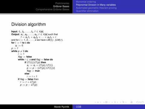
Division algorithmInput: f1, f2, . . . , fs, f ∈ k [x]Output: a1, a2, . . . , as, r ∈ k [x] such that
f = a1f1 + a2f2 + ... + as fs + rand for i = 1, 2, . . . , s we have LM(fi ) 6 |LM(r).for i := 1 to s do
ai := 0p := fwhile p 6= 0 do
i := 1flag := falsewhile i ≤ s and flag = false do
if LT (fi )˛̨LT (p) then
ai := ai + LT (p)/LT (fi )p := p − (LT (p)/LT (fi ))fiflag := true
elsei := i + 1
if flag = false thenr := r + LT (p)p := p − LT (p)
Marek Rychlik CGB

PreliminariesGröbner Bases
Comprehensive Gröbner Bases
Monomial orderingPolynomial Division in Many variablesAutomated geometric theorem provingQuantifier elimination
Ideal Membership Problem and the division algorithm
ProblemLet the variable ordering be x ≺ y ≺ z and the monomialordering be lex. Let f = z3 − y4, f1 = y2 − x3, and f2 = z − x2.Is f in the ideal Id({f1, f2})?
Marek Rychlik CGB

PreliminariesGröbner Bases
Comprehensive Gröbner Bases
Monomial orderingPolynomial Division in Many variablesAutomated geometric theorem provingQuantifier elimination
Ideal Membership Problem and the division algorithm
a1 : −y2 − x3
a2 : z2 + x2z + x4
f1 : y2 − x3
f2 : z − x2 f : z3 − y4
(f2, z2) z3 − x2z2
———————–−y4 + x2z2
(f2, x2z) x2z2 − x4z————————–
−y4 + x4z(f2, x4) x4z − x6
————————-−y4 + x6
(f1, −y2) −y4 + x3y2
————————-x6 − x3y2
(f1, −x3) −x3y2 + x6
—————0
Note: The leading terms have been underlined.
Marek Rychlik CGB

PreliminariesGröbner Bases
Comprehensive Gröbner Bases
Monomial orderingPolynomial Division in Many variablesAutomated geometric theorem provingQuantifier elimination
Ideal Membership Problem and the division algorithmThus
f = (−y2 − x3)(y2 − x3) + (z2 + x2z + x4)(z − x2)
and f ∈ I.We note that the division algorithm always produces quotientsai with the property
LT (ai fi) � LT (f ).
Marek Rychlik CGB

PreliminariesGröbner Bases
Comprehensive Gröbner Bases
Monomial orderingPolynomial Division in Many variablesAutomated geometric theorem provingQuantifier elimination
Why Gröbner Bases?The division algorithm by a random set of polynomials Fmay yield a remainder r 6= 0 even if f ∈ I.This problem does not occur if F is a Gröbner basis.
Marek Rychlik CGB

PreliminariesGröbner Bases
Comprehensive Gröbner Bases
Monomial orderingPolynomial Division in Many variablesAutomated geometric theorem provingQuantifier elimination
Notation
Let F ⊆ k [x] be an arbitrary (finite or infinite) set ofpolynomials.The leading monomial set of F is defined as
LM(F ) = {LM(f ) : f ∈ F}.
The leading term set of F is defined as
LT (F ) = {LT (f ) : f ∈ F}
If F is a polynomial ideal then so is LM(F ). Moreover, if Fis an arbitrary set then
Id(LM(F )) = LM(Id(F )).
Marek Rychlik CGB

PreliminariesGröbner Bases
Comprehensive Gröbner Bases
Monomial orderingPolynomial Division in Many variablesAutomated geometric theorem provingQuantifier elimination
Precise definition of Gröbner Bases
DefinitionA Gröbner basis is a set of polynomials G such that
LM(G) = LM(Id(G))
Equivalently, if f ∈ Id(G) then LM(f ) is divisible by LM(g) forsome g ∈ G.
Marek Rychlik CGB
PreliminariesGröbner Bases
Comprehensive Gröbner Bases
Monomial orderingPolynomial Division in Many variablesAutomated geometric theorem provingQuantifier elimination
Some properties of Gröbner BasesThe Hilbert basis theorem implies that every polynomialideal has a finite Gröbner basis.Gröbner bases can be algorithmically constructed usingBuchberger algorithm or its versions.The recent algorithms of Faugère are reported to performbetter, but they are not freely available.
Marek Rychlik CGB

PreliminariesGröbner Bases
Comprehensive Gröbner Bases
Monomial orderingPolynomial Division in Many variablesAutomated geometric theorem provingQuantifier elimination
The S-polynomial (syzygy-polynomial)
DefinitionLet f and g be two polynomials in k [x]. The syzygy polynomialof f and g is defined as follows: Let t = LCM(LT (f ), LT (g)).Then
S(f , g) =t
LT (f )f − t
LT (g)g. (1)
The above definition may differ from one in texts whichemphasize the case when k is a field: letxγ = LCM(LM(f ), LM(g)). Then
S̃(f , g) =xγ
LT (f )f − xγ
LT (g)g. (2)
Since for many applications k itself is a polynomial ring, andthus not a field, we choose to work with the first definition.
Marek Rychlik CGB

PreliminariesGröbner Bases
Comprehensive Gröbner Bases
Monomial orderingPolynomial Division in Many variablesAutomated geometric theorem provingQuantifier elimination
Buchberger Criterion
TheoremA subset G ⊆ k [x] is a Gröbner basis (of the ideal Id(G) itgenerates) iff for every f , g ∈ G we have
S(f , g)−→G
0
i.e. the remainder of division of S(f , g) by G is 0.
Marek Rychlik CGB

PreliminariesGröbner Bases
Comprehensive Gröbner Bases
Monomial orderingPolynomial Division in Many variablesAutomated geometric theorem provingQuantifier elimination
An Example of Buchberger criterion
Problem
Let V = {(t2, t3, t4) : t ∈ k}. Show thatI = I(V ) = Id({y2 − x3, z − x2}).
The solution amounts to showing that G = {g1, g2} whereg1 = y2 − x3 and g2 = z − x2, is a Gröbner basis of this idealwith variable ordering x ≺ y ≺ z and lex ordering. This can beverified using Buchberger criterion.
S(g1, g2) = z(y2 − x3)− y2(z − x2) = −x3z + x2y2
Marek Rychlik CGB

PreliminariesGröbner Bases
Comprehensive Gröbner Bases
Monomial orderingPolynomial Division in Many variablesAutomated geometric theorem provingQuantifier elimination
An Example of Buchberger criterion
Problem
Let V = {(t2, t3, t4) : t ∈ k}. Show thatI = I(V ) = Id({y2 − x3, z − x2}).
The division algorithm yields 0:a1 : x2
a2 : −x3
y2 − x3 −x3z + x2y2
z − x2 −x3z + x5
——————-x2y2 − x5
x2y2 − x5
——————-0
Thus, S(g1, g2)−→G
0, so G is a Gröbner basis.Marek Rychlik CGB

PreliminariesGröbner Bases
Comprehensive Gröbner Bases
Monomial orderingPolynomial Division in Many variablesAutomated geometric theorem provingQuantifier elimination
An Example of Buchberger criterion
Problem
Let V = {(t2, t3, t4) : t ∈ k}. Show thatI = I(V ) = Id({y2 − x3, z − x2}).
We complete the proof of I = Id(V ) by considering f ∈ I(V ). Wewrite it as f = a1f1 + a2f2 + r , where r ∈ I(V ) as well. Butr = a(x) + yb(x) because no term of r is divisible by z or y2.But the substitution x = t2, y = t3 yields a(t2) + t3b(t2). Thusa(t2) ≡ 0 and b(t2) ≡ 0 (even-odd powers). Hence a = b = 0.Also
√I = I because an ideal of a variety is always radical (k
does not have to be an algebraically closed field for thisargument to work).
Marek Rychlik CGB
PreliminariesGröbner Bases
Comprehensive Gröbner Bases
Monomial orderingPolynomial Division in Many variablesAutomated geometric theorem provingQuantifier elimination
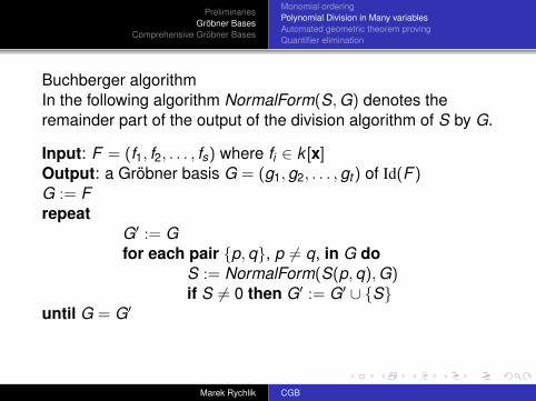
Buchberger algorithmIn the following algorithm NormalForm(S, G) denotes theremainder part of the output of the division algorithm of S by G.
Input: F = (f1, f2, . . . , fs) where fi ∈ k [x]Output: a Gröbner basis G = (g1, g2, . . . , gt) of Id(F )G := Frepeat
G′ := Gfor each pair {p, q}, p 6= q, in G do
S := NormalForm(S(p, q), G)if S 6= 0 then G′ := G′ ∪ {S}
until G = G′
Marek Rychlik CGB

PreliminariesGröbner Bases
Comprehensive Gröbner Bases
Monomial orderingPolynomial Division in Many variablesAutomated geometric theorem provingQuantifier elimination
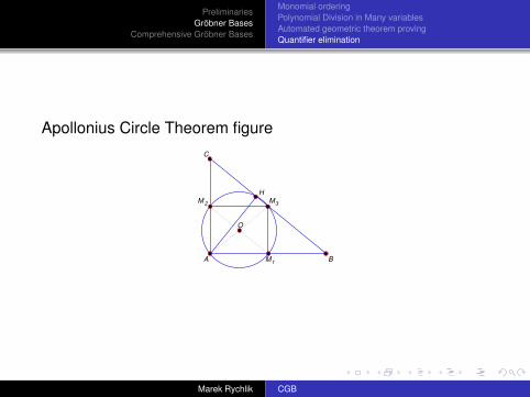
Apollonius Circle Theorem
M2
M3
A
C
BM1
O
H
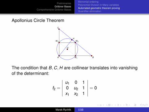
Theorem(Apollonius Circle Theorem) If ABC is a triangle, M1, M2, M3are the centers of the sides and H is the foot of the altitudedrawn from A then, M1, M2, M3 and H lie on one circle.
Marek Rychlik CGB

PreliminariesGröbner Bases
Comprehensive Gröbner Bases
Monomial orderingPolynomial Division in Many variablesAutomated geometric theorem provingQuantifier elimination
Apollonius Circle Theorem
M2
M3
A
C
BM1
O
H
Let A = (0, 0), B = (u1, 0) and C = (0, u2). Thus,
M1 = (u1
2, 0),
M2 = (0,u2
2),
M3 = (u1
2,u2
2)
are the midpoints of the sides. Let H = (x1, x2).Marek Rychlik CGB

PreliminariesGröbner Bases
Comprehensive Gröbner Bases
Monomial orderingPolynomial Division in Many variablesAutomated geometric theorem provingQuantifier elimination
Apollonius Circle Theorem
M2
M3
A
C
BM1
O
H
AM1M3M2 is a rectangle, so the circle containing A,M1,M2,M3 is
(x1 − u1/4)2 + (x2 − u2/4)2 = (u1/4)2 + (u2/4)2.
Marek Rychlik CGB

PreliminariesGröbner Bases
Comprehensive Gröbner Bases
Monomial orderingPolynomial Division in Many variablesAutomated geometric theorem provingQuantifier elimination
Apollonius Circle Theorem
M2
M3
A
C
BM1
O
H
The conditions on H are:1 AH ⊥ BC;2 B, C, H are collinear.
Marek Rychlik CGB

PreliminariesGröbner Bases
Comprehensive Gröbner Bases
Monomial orderingPolynomial Division in Many variablesAutomated geometric theorem provingQuantifier elimination
Apollonius Circle Theorem
M2
M3
A
C
BM1
O
H
The condition AH ⊥ BC translates into
f1 = (x1, x2).(u1,−u2) = 0.
Marek Rychlik CGB
PreliminariesGröbner Bases
Comprehensive Gröbner Bases
Monomial orderingPolynomial Division in Many variablesAutomated geometric theorem provingQuantifier elimination
Apollonius Circle Theorem
M2
M3
A
C
BM1
O
H
The condition that B, C, H are collinear translates into vanishingof the determinant:
f2 =
∣∣∣∣∣∣u1 0 10 u2 1x1 x2 1
∣∣∣∣∣∣ = 0
Marek Rychlik CGB

PreliminariesGröbner Bases
Comprehensive Gröbner Bases
Monomial orderingPolynomial Division in Many variablesAutomated geometric theorem provingQuantifier elimination
An algebraic fomulation of Apollonius Circle Theorem
The expanded polynomials are:
f1 = x1u1 − x2u2,
f2 = −x1u2 − u1x2 + u1u2
f = (x1 − u1/4)2 + (x2 − u2/4)2 − (u1/4)2 − (u2/4)2
= x22 − u2x2/2 + x2
1 − u1x1/2.
Apollonius Circle Theorem admits the followingreformulation:
∀u1 > 0, u2 > 0 (f1 = 0 ∧ f2 = 0) ⇒ f = 0
We can see the need to replace the above statement byone without the quantifiers.
Marek Rychlik CGB

PreliminariesGröbner Bases
Comprehensive Gröbner Bases
Monomial orderingPolynomial Division in Many variablesAutomated geometric theorem provingQuantifier elimination
“Follows strictly” Definition
DefinitionA polynomial f ∈ S follows strictly from f1, . . . , fs ∈ k [u, x] if
f ∈ Id(V (f1, . . . , fs)).
It is worth noting that this definition does not distinguishbetween parameters and variables.
Marek Rychlik CGB
PreliminariesGröbner Bases
Comprehensive Gröbner Bases
Monomial orderingPolynomial Division in Many variablesAutomated geometric theorem provingQuantifier elimination
Properties
Over algebraically closed fields, for any set of polynomialsF :
Id(V (F )) =√
Id(F ).
If k is algebraically closed then f follows strictly from F iff
f ∈√
Id({f1, f2, . . . , fs}).
If k = R then we have no simple algebraic criterion;however, if if f follows strictly over C then it follows strictlyover R.Hardly any classical geometry theorem translated into thelanguage of algebra leads to a true algebraic statement;this is due to exceptional parameters.
Marek Rychlik CGB

PreliminariesGröbner Bases
Comprehensive Gröbner Bases
Monomial orderingPolynomial Division in Many variablesAutomated geometric theorem provingQuantifier elimination
Apollonius Circle Theorem and “follows strictly”
f1 = x1u1 − x2u2,
f2 = −x1u2 − u1x2 + u1u2
f = (x1 − u1/4)2 + (x2 − u2/4)2 − (u1/4)2 − (u2/4)2
= x22 − u2x2/2 + x2
1 − u1x1/2.
We claim that f does not follow strictly from f1 and f2. Tosee it, we observe that
1 if (u, x) ∈ V ({u1, u2}) then (u, x) ∈ V ({f1, f2});2 thus, V ({u1, u2}) is a subset of V ({f1, f2});3 this means that when u1 = u2 = 0, (x1, x2) are arbitrary.
Hence, f does not have to vanish.
Marek Rychlik CGB

PreliminariesGröbner Bases
Comprehensive Gröbner Bases
Monomial orderingPolynomial Division in Many variablesAutomated geometric theorem provingQuantifier elimination
Equivalent correct reformulations
∀u1, u2(f1 = 0 ∧ f2 = 0 ∧ (u1 6= 0 ∨ u2 6= 0)
)⇒ f = 0
∀u1, u2(f1 = 0 ∧ f2 = 0 ∧ (u1u2 6= 0)
)⇒ f = 0
∀u1, u2(f1 = 0 ∧ f2 = 0
)⇒
(f = 0 ∨ u1u2 = 0
)∀u1, u2
(f1 = 0 ∧ f2 = 0
)⇒ u1u2f = 0
Quantifier-free versions:
u1u2f ∈ I(V ({f1, f2}))u1u2f ∈
√Id({f1, f2}) (k algebraically closed)
Marek Rychlik CGB

PreliminariesGröbner Bases
Comprehensive Gröbner Bases
Monomial orderingPolynomial Division in Many variablesAutomated geometric theorem provingQuantifier elimination
The saturation ideal
DefinitionGiven two ideals I, J ⊆ k [x], the saturation ideal is defined asfollows:
I : J∞ = {f ∈ k [x] : ∃g ∈ J ∃n ≥ 0 gnf ∈ I}
Marek Rychlik CGB

PreliminariesGröbner Bases
Comprehensive Gröbner Bases
Monomial orderingPolynomial Division in Many variablesAutomated geometric theorem provingQuantifier elimination
Calculating Gröbner Basis of the saturation idealGröbner basis of the saturation ideal can be computed in thesesteps:
1 Let I = Id({f1, f2, . . . , fs}) and G = Id({g1, g2, . . . , gr}.2 We form the set
F ′ = F ∪ {1− t1g1 − . . .− tr gr}
where t1, t2, . . . , tr are new variables.3 We compute the Gröbner basis H ′ of Id(F ′) with respect to
a monomial order order in which all monomials containingt ’s precede all monomials that do not depend on t ’s.
4 The subset H ⊆ H ′ of those polynomials which do notdepend on t ’s is a Gröbner basis of I : J∞.
Marek Rychlik CGB

PreliminariesGröbner Bases
Comprehensive Gröbner Bases
Monomial orderingPolynomial Division in Many variablesAutomated geometric theorem provingQuantifier elimination
Quantifier EliminationMany problems can be formulated as
∀x ∈ kn (f1(x) = 0 ∧ f2(x) = 0 ∧ . . . ∧ fp(x) = 0)
⇒ (g1(x = 0) ∨ g2(x) = 0 ∨ . . . ∨ gq(x) = 0) .
TheoremWhen k is algebraically closed, the above statement isequivalent to
1 ∈ I : J∞.
where I = Id({f1, f2, . . . , fp}) and J = Id({g1, g2, . . . , gq}).
Marek Rychlik CGB
PreliminariesGröbner Bases
Comprehensive Gröbner Bases
Monomial orderingPolynomial Division in Many variablesAutomated geometric theorem provingQuantifier elimination
Testing radical ideal membership — “Rabinowitz trick”
TheoremThe following statements are equivalent:
f ∈√
I ⇐⇒ 1 ∈ I : f∞
In other words, f belongs to the radical ideal of I iff thesaturation ideal I : f∞ is trivial.
Marek Rychlik CGB

PreliminariesGröbner Bases
Comprehensive Gröbner Bases
Monomial orderingPolynomial Division in Many variablesAutomated geometric theorem provingQuantifier elimination
CGBlisp calculations
;; An automatic proof of the Apollonius Circle Theorem;; Encoding by hand(setf vars ’(x1 x2))(setf params ’(u1 u2))(setf allvars (append vars params))(setf hypotheses "[x1*u1-x2*u2, -x1*u2-u1*x2+u1*u2]")(setf conclusions "[2*x2^2-u2*x2+2*x1^2-u1*x1,u1,u2]");; Saturation test(string-ideal-polysaturation
hypotheses conclusions allvars)
Marek Rychlik CGB

PreliminariesGröbner Bases
Comprehensive Gröbner Bases
Monomial orderingPolynomial Division in Many variablesAutomated geometric theorem provingQuantifier elimination
Calculations using CGBlisp package
USER(16): (load "../examples/apollonius0" :print 5); Loading ../examples/apollonius0.lisp(X1 X2)(U1 U2)(X1 X2 U1 U2)"[x1*u1-x2*u2, -x1*u2-u1*x2+u1*u2]""[2*x2^2-u2*x2+2*x1^2-u1*x1,u1,u2]"[ 1 ]NILT
Marek Rychlik CGB

PreliminariesGröbner Bases
Comprehensive Gröbner Bases
Monomial orderingPolynomial Division in Many variablesAutomated geometric theorem provingQuantifier elimination
A fully automated proof with CGBLisp;; Prove Apollonius Circle Theorem:(prove-theorem;; If((perpendicular A B A C) ; AB _|_ AC(midpoint B C M) ; M is the midpoint of BC(midpoint A M O) ; O is the midpoint of AM(collinear B H C) ; H lies on BC(perpendicular A H B C) ; AH _|_ BC)
;; Then((equidistant M O H O) ; MO = HO;; Or(identical-points B C) ; B = C)
)
Marek Rychlik CGB
PreliminariesGröbner Bases
Comprehensive Gröbner Bases
Monomial orderingPolynomial Division in Many variablesAutomated geometric theorem provingQuantifier elimination
Apollonius Circle Theorem figure
M2
M3
A
C
BM1
O
H
Marek Rychlik CGB
PreliminariesGröbner Bases
Comprehensive Gröbner Bases
SpecializationToy example analysisA robotics exampleClosing remarks
The Comprehensive Gröbner Basis framework
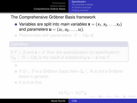
Variables are split into main variables x = (x1, x2, . . . , xn)and parameters u = (u1, u2, . . . , ul).Polynomials with parameters: S = k [u, x]
Definition
If F ⊆ S and a ∈ k l then the specialization (or specification)Fm ⊆ R = k [x] is the result of substituting u = a into F .
If G ⊆ S is a Gröbner basis then Ga ⊆ R is not a Gröbnerbasis in general.It is true that
Id(Fa) = Id(F )a
Marek Rychlik CGB

PreliminariesGröbner Bases
Comprehensive Gröbner Bases
SpecializationToy example analysisA robotics exampleClosing remarks
The Comprehensive Gröbner Basis framework
Variables are split into main variables x = (x1, x2, . . . , xn)and parameters u = (u1, u2, . . . , ul).Polynomials with parameters: S = k [u, x]
Definition
If F ⊆ S and a ∈ k l then the specialization (or specification)Fm ⊆ R = k [x] is the result of substituting u = a into F .
If G ⊆ S is a Gröbner basis then Ga ⊆ R is not a Gröbnerbasis in general.It is true that
Id(Fa) = Id(F )a
Marek Rychlik CGB

PreliminariesGröbner Bases
Comprehensive Gröbner Bases
SpecializationToy example analysisA robotics exampleClosing remarks
Comprehensive Gröbner Basis definition
DefinitionA subset G ⊆ k [u, x] is called a Comprehensive GroöbnerBasis (CGB) if for every parameter a ∈ k l Ga is a GröbnerBasis.
Theorem(Weispfenning, 1990) Every ideal I ⊆ k [u, x] has a CGB.
Marek Rychlik CGB

PreliminariesGröbner Bases
Comprehensive Gröbner Bases
SpecializationToy example analysisA robotics exampleClosing remarks
The toy example
-
6
@@
@@
@@@
BB
BB
BB
BB
-
6
@@
@@
@@@
x + y = 0
ux + y = 0
x
y u 6= 1
x + y = 0
x
y u = 1
ux + y = 0
Problem(Toy problem in CGB) What is the dimension of the intersectionof two lines x + y = 0 and ux + y = 0 as function of theparameter u?
Marek Rychlik CGB

PreliminariesGröbner Bases
Comprehensive Gröbner Bases
SpecializationToy example analysisA robotics exampleClosing remarks
The toy example
-
6
@@
@@
@@@
BB
BB
BB
BB
-
6
@@
@@
@@@
x + y = 0
ux + y = 0
x
y u 6= 1
x + y = 0
x
y u = 1
ux + y = 0
Let F = {x + y , ux + y} ⊂ k [u, x , y ]
Let us first find the Gröbner basis as a function of theparameter (x � y � z, the monomial order is lex).We run into a problem: we are not able to determine whatthe LM(ux + y) is.We need to branch the computation.
Marek Rychlik CGB

PreliminariesGröbner Bases
Comprehensive Gröbner Bases
SpecializationToy example analysisA robotics exampleClosing remarks
The tree generated by the CGB algorithm
��
���
@@
@@@R
��
��
��
SS
SS
SSw
{x + y , ux + y}
u = 0
{x + y , ux + y , (u − 1)y}
{x + y , ux + y , (u − 1)y}
{x + y , ux + y}
u 6= 0
{x + y , ux + y , (u − 1)y}
u = 1 u 6= 1
Marek Rychlik CGB

PreliminariesGröbner Bases
Comprehensive Gröbner Bases
SpecializationToy example analysisA robotics exampleClosing remarks
The solution of a parametric problem
The Comprehensive Gröbner System (CGS) is an objectderived from the algorithmically constructed tree previouslyconsidered.For the toy example,
{ ( { u = 0 }, { x + y , ux + y } ),
( { u 6= 0, u = 1 }, { ux + y , (u − 1)y} ),
( { u 6= 0, u 6= 1 }, { ux + y , (u − 1)y} ) }.
Marek Rychlik CGB

PreliminariesGröbner Bases
Comprehensive Gröbner Bases
SpecializationToy example analysisA robotics exampleClosing remarks
Comprehensive Gröbner System DefinitionA Comprehensive Gröbner System consists of pairs.The first element is a condition, i.e. a set of equations(green list) and inequations (red list) obtained by walkingdown from the root of the tree to the leaf.The second element of each pair is a Gröbner basis underany specialization satisfying the condition (leaf of the tree).
Marek Rychlik CGB

PreliminariesGröbner Bases
Comprehensive Gröbner Bases
SpecializationToy example analysisA robotics exampleClosing remarks
Mathematical robotics
θ3
x
y
θ1
θ2
`2
`3
`4
(a, b)
Joint space: J = {(θ1, θ2, . . . , θm)}Configuration space: C = {(a, b)}Joint map: f : J → CKinematic singularity: when joint is moving with infinitevelocity while the grasper is moving with finite velocity.
Marek Rychlik CGB

PreliminariesGröbner Bases
Comprehensive Gröbner Bases
SpecializationToy example analysisA robotics exampleClosing remarks
Dimension analysis of the joint map
Problem
Determine the dimensions of the varieties f−1(c) for all points cfor the two-arm robot with l2 = l3 = 1.
Marek Rychlik CGB
PreliminariesGröbner Bases
Comprehensive Gröbner Bases
SpecializationToy example analysisA robotics exampleClosing remarks
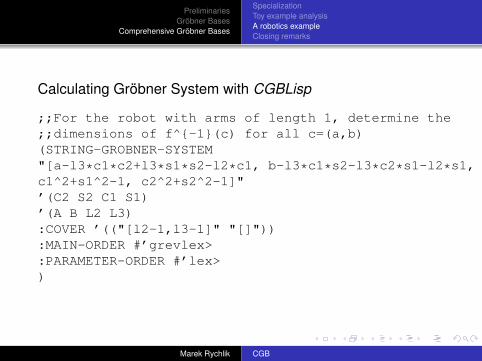
Calculating Gröbner System with CGBLisp
;;For the robot with arms of length 1, determine the;;dimensions of f^{-1}(c) for all c=(a,b)(STRING-GROBNER-SYSTEM"[a-l3*c1*c2+l3*s1*s2-l2*c1, b-l3*c1*s2-l3*c2*s1-l2*s1,c1^2+s1^2-1, c2^2+s2^2-1]"’(C2 S2 C1 S1)’(A B L2 L3):COVER ’(("[l2-1,l3-1]" "[]")):MAIN-ORDER #’grevlex>:PARAMETER-ORDER #’lex>)
Marek Rychlik CGB

PreliminariesGröbner Bases
Comprehensive Gröbner Bases
SpecializationToy example analysisA robotics exampleClosing remarks
NotesThe settings l2 = l3 = 1 are included as part of the greenlist instead of modifying the equationsThe main variable order is set to grevlex.The order must be a graded order in order to calculate thedimension.
Marek Rychlik CGB

PreliminariesGröbner Bases
Comprehensive Gröbner Bases
SpecializationToy example analysisA robotics exampleClosing remarks
A theorem on dimension
TheoremIf a graded monomial order is used then:
dim(V (I)) = dim(V (LM(I))).
If I is a monomial ideal then the variety V (I) is a union ofcoordinate hyperplanes.The dimension dim(V (I)) can be easily computed.
Marek Rychlik CGB

PreliminariesGröbner Bases
Comprehensive Gröbner Bases
SpecializationToy example analysisA robotics exampleClosing remarks
Output of CGBLisp - Case 1
-------------------CASE 1-------------------Condition:Green list: [L2-1,L3-1]Red list: [A,A^2+B^2]Basis: [(-2*A)*S2+(-2*A^2-2*B^2)*S1+(A^2*B+B^3),(-2)*C2+(A^2+B^2-2),(2*A)*C1+(2*B)*S1+(-A^2-B^2),(4*A^2+4*B^2)*S1^2+(-4*A^2*B-4*B^3)*S1+(A^4+2*A^2*B^2-4*A^2+B^4)]
Marek Rychlik CGB

PreliminariesGröbner Bases
Comprehensive Gröbner Bases
SpecializationToy example analysisA robotics exampleClosing remarks
Output of CGBLisp - Case 2
-------------------CASE 2-------------------Condition:Green list: [L2-1,L3-1,A^2+B^2]Red list: [B^2,A]Basis: [(32*B^4)]
Marek Rychlik CGB
PreliminariesGröbner Bases
Comprehensive Gröbner Bases
SpecializationToy example analysisA robotics exampleClosing remarks
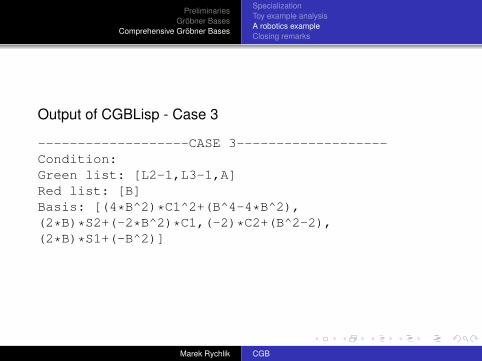
Output of CGBLisp - Case 3
-------------------CASE 3-------------------Condition:Green list: [L2-1,L3-1,A]Red list: [B]Basis: [(4*B^2)*C1^2+(B^4-4*B^2),(2*B)*S2+(-2*B^2)*C1,(-2)*C2+(B^2-2),(2*B)*S1+(-B^2)]
Marek Rychlik CGB

PreliminariesGröbner Bases
Comprehensive Gröbner Bases
SpecializationToy example analysisA robotics exampleClosing remarks
Output of CGBLisp - Case 4
-------------------CASE 4-------------------Condition:Green list: [L2-1,L3-1,A,B]Red list: []Basis: [(1)*C1^2+(1)*S1^2+(-1),(1)*S2,(1)*C2+(1)]
Marek Rychlik CGB

PreliminariesGröbner Bases
Comprehensive Gröbner Bases
SpecializationToy example analysisA robotics exampleClosing remarks
Dimension of the kinematic singularityThe dimension ccan be calculated automatically, but wecan do it by hand easily as well.The following table contains the necessary information:
Case # LM(I) dimension1 Id({s2, c2, c1, s2
1}) 02 Id({1}) -13 Id({c2
1 , s2, c2, s1}) 04 Id({c2
1 , s2, c2}) 1
Marek Rychlik CGB

PreliminariesGröbner Bases
Comprehensive Gröbner Bases
SpecializationToy example analysisA robotics exampleClosing remarks
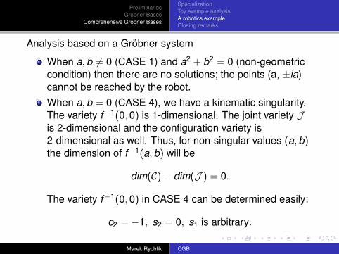
Analysis based on a Gröbner system
When a, b 6= 0 (CASE 1) and a2 + b2 = 0 (non-geometriccondition) then there are no solutions; the points (a, ±ia)cannot be reached by the robot.When a, b = 0 (CASE 4), we have a kinematic singularity.The variety f−1(0, 0) is 1-dimensional. The joint variety Jis 2-dimensional and the configuration variety is2-dimensional as well. Thus, for non-singular values (a, b)the dimension of f−1(a, b) will be
dim(C)− dim(J ) = 0.
The variety f−1(0, 0) in CASE 4 can be determined easily:
c2 = −1, s2 = 0, s1 is arbitrary.
Marek Rychlik CGB
PreliminariesGröbner Bases
Comprehensive Gröbner Bases
SpecializationToy example analysisA robotics exampleClosing remarks
Into the futureStudy papers of Faugère to get to the forefront of currentresearch on GB, especially the F4 and F5 algorithms.Akiro Suzuki described an algorithm for CGB which usesonly standard GB and a clever choice of slack variables.Kuranishi-Cartan theory studies mildly non-commutativerings, when some “variables” are differential operators.Interesting applications to PDE are on the horizon. StudyG. Reid, Ping Lin, A. Wittkopf and W.M. Seiler.
Marek Rychlik CGB
Top Related