


Languages
Pages
Legal


Student thesis series INES nr 392
SHUZHI DONG
2016
Department of
Physical Geography and Ecosystem Science
Lund University
Sölvegatan 12
S-223 62 Lund
Sweden
Comparisons between Different
Multi-criteria Decision Analysis Techniques
for Disease Susceptibility Mapping

i
Shuzhi Dong (2016).
Comparisons between Different Multi-criteria Decision Analysis Techniques for Disease
Susceptibility Mapping
Master degree thesis, 30 credits in Geomatics
Department of Physical Geography and Ecosystem Science, Lund University
Level: Master of Science (MSc)
Course duration: January 2016 until June 2016

ii
Comparisons between Different Multi-criteria Decision
Analysis Techniques for Disease Susceptibility Mapping
Author
SHUZHI DONG
Master thesis, 30 credits, in Geomatics
Supervisor Ali Mansourian
Co-Supervisor Mohammadreza Rajabi
Department of physical Geography and Ecosystem Science in Lund University
Exam committee: Ehsan Abdolmajidi
Examiner Hasan Abdulghani
Department of physical Geography and Ecosystem Science in Lund University

iii
Abstract
Geographic information system multi-criteria decision analysis (GIS-MCDA) procedure can
combine criterion maps together and associated the criterion weights to acquire an overall
value for each spatial location in the research area. Analytical Hierarchy Process (AHP),
Technique for Order of Preference by Similarity to Ideal Solution (TOPSIS), Ordered Weighted
averaging (OWA) are three generic algorithms of multi-criteria decision analysis. These have
been combined with GIS to tackle wide range of spatial problems.
In this research, the comparison of AHP, TOPSIS, and OWA methods for susceptibility
mapping in spatial communicable disease study had been made through testing the
sensitivity of each model. The methods are compered by two concrete case studies:
modelling of visceral leishmaniasis in north-western Iran for mapping of risky areas and
modelling of dengue disease in Ecuador for mapping of risky areas. In regard to testing the
algorithms, prediction-rate method was utilized to draw the receiver operating characteristic
(ROC) curve. Comparing the tendency of ROC curves and the risk-prone areas of the disease
from susceptibility maps, also considering the realistic situations of two infectious diseases,
evaluations of these three algorithms had been done.
In this research, at least in this application, AHP model offers the best predictive accuracy in
both of these two case studies.
Keywords: multi-criteria decision analysis, AHP, TOPSIS, OWA, disease susceptibility mapping

iv
Acknowledgements
First of all, the first appreciation and gratitude is to my supervisor Ali Mansourian. Without
his explanations and guidance, this thesis could not have been possible. He allowed me by
his willing to focus on health-GIS study area and I hope that I could expend and spread the
knowledge I obtained from this study in every possible way.
Great thanks to Mohammadreza Rajabi who provide the VL disease data from Northwest
Iran for me. During the developing of the models, Rajabi had given me so many useful
suggestions. He has not spared any possible help.
Thanks to Viviana Paola Santander Rodriguez for providing me dengue data from Ecuador,
her friendship and company will be imprinted in my mind.
The greatest and most gratitude thanks for my parents, my father and mother being always
there for me with all their support and feelings. I cannot express how much respect and love
I bear in my heart to my parents. I would not suffice just a bit of what they have offered me
during the past twenty years of my life also the future years.
v
Table of Contents
STUDENT THESIS SERIES INES NR XX ........................................................................................................
ABSTRACT ............................................................................................................................................... III
ACKNOWLEDGEMENTS .......................................................................................................................... IV
TABLE OF CONTENTS ............................................................................................................................... V
LIST OF ACRONYMS ............................................................................................................................... VII
LIST OF FIGURES ................................................................................................................................... VIII
LIST OF TABLES ....................................................................................................................................... IX
CHAPTER 1............................................................................................................................................... 1
1. INTRODUCTION ............................................................................................................................... 1
1.1 BACKGROUND ......................................................................................................................... 1
1.2 RESEARCH OBJECTIVES ............................................................................................................... 2
1.3 METHODOLOGY ....................................................................................................................... 2
1.4 OUTLINE ................................................................................................................................ 2
CHAPTER 2............................................................................................................................................... 3
2. LITERATURE REVIEW ........................................................................................................................ 3
2.1 GIS IN HEALTH STUDY (SPATIAL EPIDEMIOLOGY) ............................................................................... 3
2.2 MULTI-CRITERIA DECISION ANALYSIS TECHNIQUES ............................................................................. 3
2.2.1 ANALYTICAL HIERARCHY PROCESS (AHP) ........................................................................................... 4
2.2.2 TECHNIQUE FOR ORDER OF PREFERENCE BY SIMILARITY TO IDEAL SOLUTION (TOPSIS) ............................. 6
2.2.3 ORDERED WEIGHTED AVERAGING (OWA) .......................................................................................... 8
CHAPTER 3............................................................................................................................................. 12
3. IMPLEMENTATION ......................................................................................................................... 12
3.1 STUDY AREA ......................................................................................................................... 14
3.3 VL DISEASE IN NORTHWEST IRAN ............................................................................................... 14
3.3.1 AHP RESULTS AND MAP ................................................................................................................. 14
3.3.2 TOPSIS RESULTS AND MAP ............................................................................................................. 19
3.3.3 OWA RESULTS AND MAPS .............................................................................................................. 21
3.4 DENGUE DISEASE IN ECUADOR .................................................................................................. 27
3.4.1 AHP RESULTS AND MAP ................................................................................................................. 27
3.4.2 TOPSIS RESULTS AND MAP ............................................................................................................. 28
3.4.3 OWA RESULTS AND MAP ................................................................................................................ 29
CHAPTER 4............................................................................................................................................. 33
vi
4. RESULTS AND DISCUSSION ............................................................................................................ 33
4.1 VALIDATION OF MODELS USED ................................................................................................... 33
4.1.1 VL DISEASE IN NORTHWEST IRAN ..................................................................................................... 33
4.1.2 DENGUE DISEASE IN ECUADOR ........................................................................................................ 37
4.2 LIMITATION ........................................................................................................................... 40
CHAPTER 5............................................................................................................................................. 41
5. CONCLUSION .................................................................................................................................. 41
REFERENCE ............................................................................................................................................ 42
APPENDIX .............................................................................................................................................. 46
QUESTIONNAIRES FOR VL DISEASE ...................................................................................................... 46
AHP METHOD ..................................................................................................................................... 46
TOPSIS AND OWA METHOD ................................................................................................................. 50
QUESTIONNAIRES FOR DENGUE DISEASE ............................................................................................... 51
AHP METHOD ..................................................................................................................................... 51
TOPSIS AND OWA METHOD ................................................................................................................. 53
vii
List of Acronyms
AHP Analytical Hierarchy Process
AUC Area Under the ROC curve
CI Consistency Index
CR Consistency Ratio
DEX Decision Expert
DF Dry Farm
DMs Decision Makers
FC Forest with Canopy Cover
FN False Negative Fraction
FP False Positive Fraction
GIS Geographic Information System
GIScience Geographic information science
IF Irrigated Farming and Orchards
ITDRC Infectious and Tropical Diseases Research Center
LR Lakes and Water Reservoirs
MCDA Multi Criteria Decision Analysis
MoH Ministry of Health
NIS Negative Ideal Solution
OWA Ordered Weighted averaging
PAHO Pan American Health Organization
PIS Positive Ideal Solution
RC Rangelands with Canopy Cover
RB Large River Beds
ROC Receiver Operating Characteristic
ST Health Center Nomads and Settlement
TN True Negative Fraction
TOPSIS Technique for Order of Preference by Similarity to Ideal Solution
TP Ture Positive Fraction
VL Visceral Leishmaniasis
WLC Weighted Linear Combination
viii
List of Figures
Figure 2-1.Knowledge driven Vs Data driven .................................................................................................. 4
Figure 2-2.AHP process flow chart (Saaty and Vargas 1991) .......................................................................... 5
Figure 2-3.TOPSIS process flow chart .............................................................................................................. 7
Figure 2-4.The OWA process flow chart ........................................................................................................11
Figure 3-1.Factors maps of VL disease in northwest Iran .............................................................................13
Figure 3-2.Factors maps of dengue disease in Ecuador (mainland)..............................................................13
Figure 3-3.(1) Study area in East Azerbaijian,Iran; (2)Study area in the mainland of Ecuador. ....................14
Figure 3-4.APH hierarchy associated with VL ................................................................................................15
Figure 3-5.Susceptibility map of VL in northwest Iran by AHP .....................................................................18
Figure 3-6.Susceptibility map of VL in northwest Iran by TOPSIS .................................................................21
Figure 3-7.Flow chart of OWA .......................................................................................................................22
Figure 3-8.Susceptibility map of VL in northwest Iran by OWA0 method ....................................................24
Figure 3-9. Susceptibility map of VL in northwest Iran by OWA0.1 method ................................................24
Figure 3-10. Susceptibility map of VL in northwest Iran by OWA0.4 method ..............................................25
Figure 3-11. Susceptibility map of VL in northwest Iran by OWA1 method .................................................25
Figure 3-12. Susceptibility map of VL in northwest Iran by OWA2 method .................................................26
Figure 3-13.Susceptibility map of VL in northwest Iran by OWA10 method ................................................26
Figure 3-14.Susceptibility map of VL in northwest Iran by OWA∞ method ...............................................27
Figure 3-15.Susceptibility map of Dengue in Ecuador by AHP ......................................................................28
Figure 3-16.Susceptibility map of dengue in Ecuador by TOPSIS ..................................................................29
Figure 3-17.Susceptibility map of dengue in Ecuador by OWA0 ..................................................................30
Figure 3-18. Susceptibility map of dengue in Ecuador by OWA0 ..................................................................31
Figure 3-19.Susceptibility map of dengue in Ecuador by OWA1 ..................................................................31
Figure 3-20. Susceptibility map of dengue in Ecuador by OWA2 ..................................................................32
Figure 3-21.Susceptibility map of dengue in Ecuador by OWA10 ................................................................32
Figure 3-22. Susceptibility map of dengue in Ecuador by OWA ∞ ..............................................................33
Figure 4-1.AHP multiclass susceptibility map with validation points for VL .................................................35
Figure 4-2.The ROC curves for AHP, TOPSIS, OWA 0.4, WLC .........................................................................36
Figure 4-3.AHP multiclass susceptibility map with validation areas for dengue ..........................................38
Figure 4-4 .The ROC curves for AHP, TOPSIS, OWA 0.4, WLC ........................................................................39
ix
List of Tables
Table 2-1.Scales for pairwise comparisons (Saaty 2008) ................................................................................ 6
Table 2-2.The decision strategies corresponding to specific ORness Value (Jelokhani-Niaraki 2015) ..........10
Table 3-1.Pairwise comparison matrix, factor weights and consistency ratio of the data layers used .........16
Table 3-2.Pairwise comparison matrix for dataset layers of VL analysis .......................................................17
Table 3-3.Factors weights for TOPSIS model .................................................................................................19
Table 3-4.The PIS NIS and ideal closeness value in TOPSIS model(pick 20 of 8145 figures as example) ......20
Table 3-5.Optimal order weights for selected values of the parameter α and the number of map layers. .22
Table 3-6.Some properties for selected values of the α parameter (Jelokhani-Niaraki 2015) .....................23
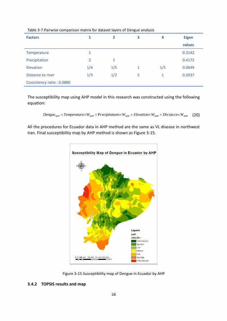
Table 3-7.Pairwise comparison matrix for dataset layers of Dengue analysis ..............................................28
Table 3-8.Factors weights for TOPSIS model (Dengue) .................................................................................29
Table 3-9.Order weights for selected values of the parameter α and trade-off values ................................30
Table 4-1.Areas under category (%) for each method ..................................................................................34
Table 4-2.Validation data used for AHP, TOPSIS, OWA 0.4, WLC ...................................................................36
Table 4-3.AUC values of TOPSIS,AHP, OWA 0.4, WLC for VL disease in northwest Iran ................................37
Table 4-4.Areas under category (%) for each method ..................................................................................37
Table 4-5.Validation data used for AHP, TOPSIS, OWA 0.4, WLC ...................................................................38
Table 4-6.AUC values of TOPSIS, AHP, OWA 0.4 WLC for Dengue disease in Ecuador ..................................39

1
Chapter 1
1. Introduction
1.1 Background
Global changes in earth system influences patterns of human health, international health
care, and public health activities (McMichael 2013). Specifically, some vector borne diseases
like communicable diseases always reminded as global disease burden. GIS are being used
with enhancive frequency in spatial epidemiology researches. As advances GIS technology
make it much easier to connect spatially referenced physical and social-economic
phenomena to patterns of health, disease and well-being (Krieger 2003). Disease risk
mapping has become an established technique in spatial epidemiology study, it aims to
summarize spatial and geographical variations in disease risk, for purpose of assessing and
quantifying the amount of true spatial heterogeneity and the associated patterns, to
highlight areas of elevated or lower risk and to obtain clues as to disease etiology (Best,N., et
al. 2005). Descriptive disease risk mapping aims at illustrating the spatial variation, the data
being used in these maps are always earned by surveys or surveillance. For the existing
data-sparse situations, GIS-based multi-criteria decision analysis (GIS-MCDA) can be used to
analysis the disease risk maps. The variety of influencing factors (criteria) and the need to
use experts’ knowledge on how to integrate these factors is also the main reason for using
MCDA.
Combination of GIS and MCDA gives decision makers not only the single strategy for
geographical region but also different weights for different strategies. Many spatial decision
problems lead to the GIS-based multi-criteria decision analysis. Spatial analysis and decision
support systems provide perspectives among both MCDA and GIS, concept of totalization
GIS and MCDA contribute a lot to the GIScience development. The integration between GIS
and multi-criteria decision analysis (MCDA), had significantly developed over the last 25
years. GIS plays an essential role in decision problem analysis. In the same time, MCDA also
provide a rich mixture of procedures to structure the decision problems, among this the
alternative decisions will be designed and evaluated (Malczewski 2006). Indeed, most of the
fundamental level GIS-MCDA is processed as the transformation and combination of
geographical data and criteria judgement (which comes from the decision maker’s
preferences), in order to achieve successful decision making. Using GIS-based MCDA
methods for health-GIS application improve the understanding of uncertainties surroundings.
With this in mind, in this research, MCDA technique was selected to deal with the
influencing factors in the disease risk mapping.
Susceptibility maps combine different factors that contribute to a hazard together, aimed at
achieving the most likely occurred hazard area; it can understand and predict future hazards,
based on statistical or deterministic methods. Mapping the areas that are susceptible to
some existed disasters or diseases is essential for effective management and can control the
spread of the damage cause by them. It could be the basis for decision maker to help people
2
reduce the losses caused by disasters or diseases. In a creation of susceptibility map,
mapping method integrates many factors and weights the importance of different variables,
using subjective decision-making rules, based on the experience of the experts involved
(Zhu,L. and Huang,J.F.2006). The GIS-based MCDA methods can be used to solve the factors
and weights problems during creating susceptibility map.
In order to find an efficient method to obtain high accuracy disease susceptibility maps, we
test three models to solve this problem. The three models being implemented in this
research are AHP, TOPSIS, and OWA respectively.
1.2 Research objectives
(1) The main objective of this study is to use three of GIS-MCDA methods namely Analytical
Hierarchy Process (AHP), Technique for Order of Preference by Similarity to Ideal Solution
(TOPSIS) and Ordered Weighted averaging (OWA), in susceptibility mapping.
(2) Secondary aims of this study were to compare these three methods by analyzing the
difference between their potential risks of diseases shown from the susceptibility
mapping. To discuss the suitability one of the techniques for disease risk prediction from
these three methods.
1.3 Methodology
To investigate the status and risk level of the disease, experts and physicians’ knowledge
were directly entered into these three models. The algorithms were developed in MATLAB to
achieve values in each model. All the data tested by these three models were produced in
ArcGIS.
To obtain the weights for these methods, questionnaires of the factors firstly sent to the
experts. Questionnaire for each method is in the appendix; OWA and TOPSIS have the same
questionnaire. AHP method has different one, pairwise comparison was used in this
questionnaire. Factors were identified via literature review. To test the liability of the models,
two case studies, visceral leishmaniasis (VL) in north-western Iran and dengue disease in
Ecuador were used for testing. In order to validate these three models, prediction-rate
method was used, the results of the susceptibility maps from different models, were
validated by comparing them with the existing infected areas. ROC curves of the three
models were draw to analyze the models in statistical level.
1.4 Outline
This thesis is organized in 5 chapters. Chapter 1 is introduction, which includes background,
research objectives, methodology and outline. Chapter 2 is literature review, which contains
both GIS for health study and MCDA techniques. In GIS health study section, the
development and combination of GIS and health study was introduced. In MCDA techniques
segment, the three methods AHP, TOPSIS, OWA were introduced by detail. Chapter 3 is
implementation, two cases: VL disease in northwest Iran and dengue disease in Ecuador
were used for implement the models. In chapter 4, validations and discussions about the
three models were drawn. In final chapter, conclusions of the all studies were presented.

3
Chapter 2
2. Literature review
2.1 GIS in health study (spatial epidemiology)
Communicable disease study is the study of health and disease in human populations, time,
person, place are the first 3 important epidemiologic variables in this analysis; place,
however always been the most difficult one to illustrate (Melnick Al, et al. 1999). Spatial
analysis methods and GIS has been combined together to enhance the understanding and
visualization of spatial and health data. GIS in spatial epidemiology study is a field dealing
with spatial (spatial-temporal) data that linked to the disease spread or population at risk.
The objective of spatial epidemiology study is to identify disease causes and correlates by
relating spatial disease patterns to geographic variation in health risks (Jacquez,G.M. 2000).
Disease mapping studies have become an established technique in health GIS study, which
aims to summarize spatial variation in disease risk to assess and quantify the spatial
heterogeneity, highlight areas of risk area and to gain the disease prediction. When applying
spatial communicable disease analysis methods as part of disease management to forecast
and assess the potential of the disease, the information decision makers expect to acquire
from risk includes both the level of disease risk and information on risk factors.
For the modelling techniques, it can be categorized into two kinds of methods: data-driven
and knowledge-driven. The former one is characterized by statistical methods to define
relationships between factors and disease risk, however the later approach is based on
existing knowledge about the relationships with the disease risk of interest. Receiving and
integrating the knowledge of experts is very important and challenging, knowledge-driven
techniques provide the solutions for this problem. It is useful for identifying risk factors,
which also means the statistical regression models that being used in knowledge-driven
approach eliminate proxy risk factor variables related to unobserved disease transmission
procedures. Transmission dynamics can be directly modelled in knowledge-driven
techniques. More detailed description about knowledge-driven techniques is discussed in
2.2.
2.2 Multi-criteria decision analysis techniques
Multi-criteria decision analysis (MCDA) considers multiple criteria together into the
decision-making environment; it is a sub-discipline of operations research. A variety of
approaches and methods have been already developed for the implementation of MCDA in
an array of disciplines, which range from social science to natural science. There is a large
number of methods in MCDA, for instance, Analytic hierarchy process(AHP),Decision Expert
(DEX), Data envelopment analysis, Technique for the order of Preference by Similarity to
Ideal Solution(TOPSIS),etc. More than 33 methods can be listed for conducting MCDA.
However many of them are applied on a small number of alternatives, due to the limitation
in computation or practice (Greene et al. 2011). Spatial decision problem can also be sloved
by the implementation of MCDA. Spatial decision problem involves a huge set of alternatives

4
are often evaluated by decision-makers, managers, stake-holders, etc.
MCDA is knowledge-driven technique. Different from data-driven technique, the activity
progress in knowledge-driven technique is not compelled by data. In knowledge-driven
technique, the generation and use of knowledge is the major part in the creation of the
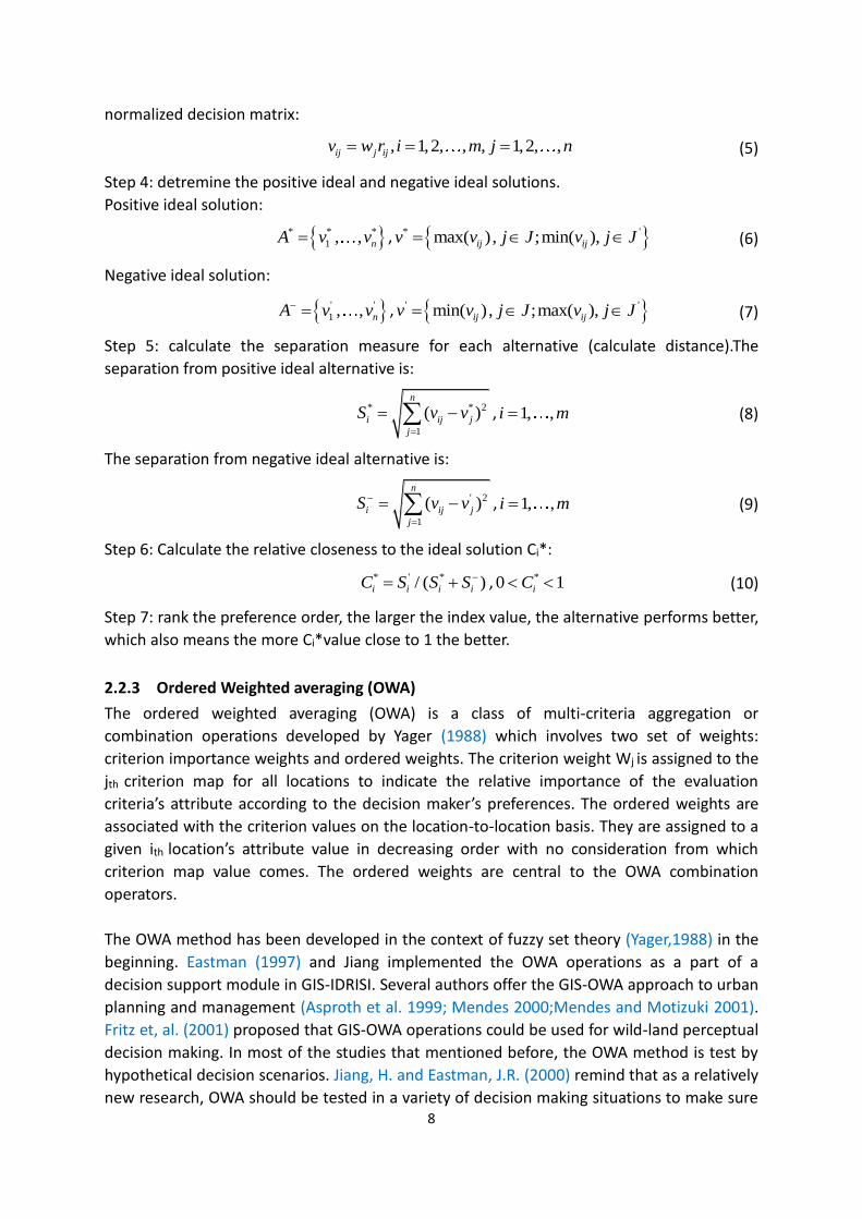
procedure (Figure2-1). In this study, three GIS-MCDA models were implemented, which were
AHP, TOPSIS and OWA.
KnowledgeDrivenprocess
DataDrivenProcess
Experience Research
Big DataBig Data
Figure 2-1.Knowledge driven Vs Data driven
AHP is a structured technique for organizing and analyzing complex decisions, based
on mathematics and psychology developed by Thomas L. Saaty in the 1970s and has been
extensively studied and refined since then. TOPSIS is a multi-criteria decision
analysis method, which was originally developed by Hwang and Yoon in 1981 and further
developed by Yoon in 1987, and Hwang, Lai and Liu in 1994.The ordered weighted averaging
(OWA) operators provide a parameterized class of mean type aggregation operators. They
approved by Ronald R.Yager(1988). Many notable mean operators such as max, arithmetic
average, median and min, are members of this class.
2.2.1 Analytical Hierarchy Process (AHP)
AHP method (Saaty 1977, 1980; Saaty and Vargas 1991) is a well-known method in
multi-criteria techniques, which has been incorporated into GIS-based suitability procedure
(Marinoni 2004; Jankowski and Richard 1994). In this method, both quantitative and
qualitative information about decision-making problems can be organized (Saaty 1980;
Malczewski 1999). AHP is a flexible, quantitative method for selecting among alternatives
which are based on their relative performance to more than one interest criteria
(Boroushaki and Malczewki 2008; Linkov et al. 2007). The ratio scales of criteria can be
driven from paired comparison in AHP method. After the weights were determined through
the pairwise comparison method, the resulting evaluation scores are used to order the
decision alternatives from the most to the least desirable, followed by an aggregation
criterion technique (Jiang and Eastman 2000; Gorsevski et al. 2006).
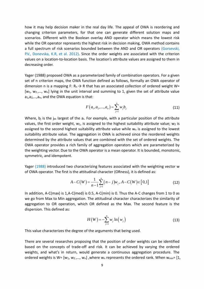
As a structured technique organizing analyzing complex decisions based on mathematics
and psychology, the AHP method works as a flow chart (Figure 2-2) (Saaty and Vargas 1991).
Step 1, define alternatives: define the complete list of alternatives which come from your
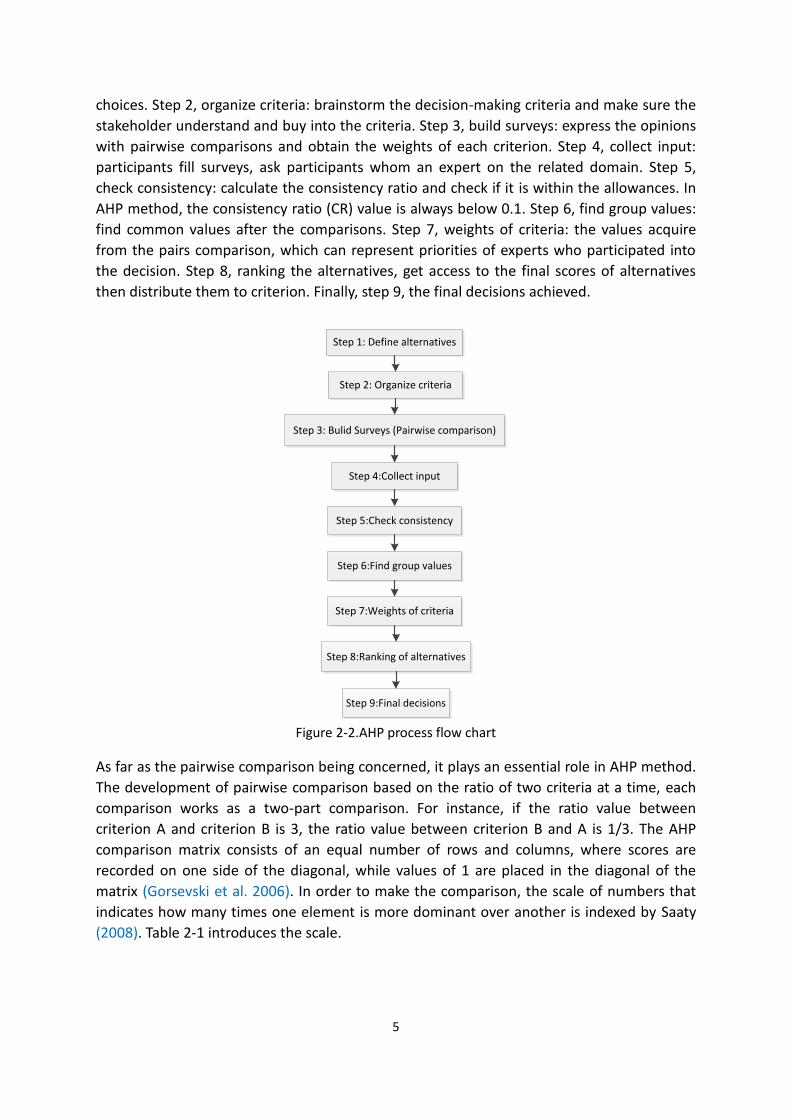
5
choices. Step 2, organize criteria: brainstorm the decision-making criteria and make sure the
stakeholder understand and buy into the criteria. Step 3, build surveys: express the opinions
with pairwise comparisons and obtain the weights of each criterion. Step 4, collect input:
participants fill surveys, ask participants whom an expert on the related domain. Step 5,
check consistency: calculate the consistency ratio and check if it is within the allowances. In
AHP method, the consistency ratio (CR) value is always below 0.1. Step 6, find group values:
find common values after the comparisons. Step 7, weights of criteria: the values acquire
from the pairs comparison, which can represent priorities of experts who participated into
the decision. Step 8, ranking the alternatives, get access to the final scores of alternatives
then distribute them to criterion. Finally, step 9, the final decisions achieved.
Step 1: Define alternatives
Step 2: Organize criteria
Step 3: Bulid Surveys (Pairwise comparison)
Step 4:Collect input
Step 5:Check consistency
Step 6:Find group values
Step 7:Weights of criteria
Step 8:Ranking of alternatives
Step 9:Final decisions
Figure 2-2.AHP process flow chart
As far as the pairwise comparison being concerned, it plays an essential role in AHP method.
The development of pairwise comparison based on the ratio of two criteria at a time, each
comparison works as a two-part comparison. For instance, if the ratio value between
criterion A and criterion B is 3, the ratio value between criterion B and A is 1/3. The AHP
comparison matrix consists of an equal number of rows and columns, where scores are
recorded on one side of the diagonal, while values of 1 are placed in the diagonal of the
matrix (Gorsevski et al. 2006). In order to make the comparison, the scale of numbers that
indicates how many times one element is more dominant over another is indexed by Saaty
(2008). Table 2-1 introduces the scale.

6
Table 2-1.Scales for pairwise comparisons (Saaty 2008)
Intensity of
importance
Description Explanation
1 Equal importance Two activities contributes equally to the object
2 Weak or slight
3 Moderate importance Experience and judgement slightly favour one
activity over another
4 Moderate plus
5 Strong importance Experience and judgement strongly favour one
activity over another
6
7
8
9
Strong plus
Very strong or
demonstrated importance
Very, very strong
Extreme importance
An activity is favoured very strongly over another,
its dominance demonstrated in practice
The evidence favouring one activity over another is
of the highest possible order of affirmation
Reciprocals Values for inverse comparison A reasonable assumption
Human judgment sometimes can violate the transitivity rule and thus cause an inconsistency;
therefore the consistency ratio (CR) is computed to check the consistency of the conducted
comparisons (Gorsevski et al. 2006). If the comparison matrix is neither totally consistent
nor contradictory, a different situations will appears ,to solve this, one suitable
measurement was described by Saaty(1980), the consistency index(CI) is calculated as
follows:
CI =
λmax − n
n − 1 (1)
Where, λmax is the biggest principal eigenvalue, n is the number of compared alternatives.
Occasionally, the referee is not absolutely consistent; Saaty defined the consistency ratio (CR)
to measure this level of inconsistency:
CR =
CI
RI (2)
Where RI is random index, this value can be obtained from a lookup table. Saaty had
required that only the CR value below 0.1 is acceptable.
2.2.2 Technique for Order of Preference by Similarity to Ideal Solution (TOPSIS)
TOPSIS, originally developed by Hwang and Yoon (1981), is a crucial MCDA method which is
widely used in different decision making problems. The basic concept of TOPSIS contains the
chosen of the shortest geometric distance between alternative and positive ideal solution
(PIS), and the longest geometric distance between alternative and negative ideal solution
7
(NIS). According to this the original idea of TOPSIS is straightforward: originates from the
concept of a displaced ideal point from the compromise solution with the shortest
distance(Belenson, S.M.,Kapur, K.C), both the distance to positive ideal solution and negative
ideal solution being considered simultaneously by TOPSIS . The final ranking is obtained by
means of the closeness index.
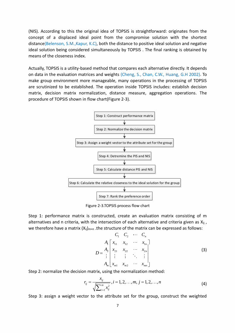
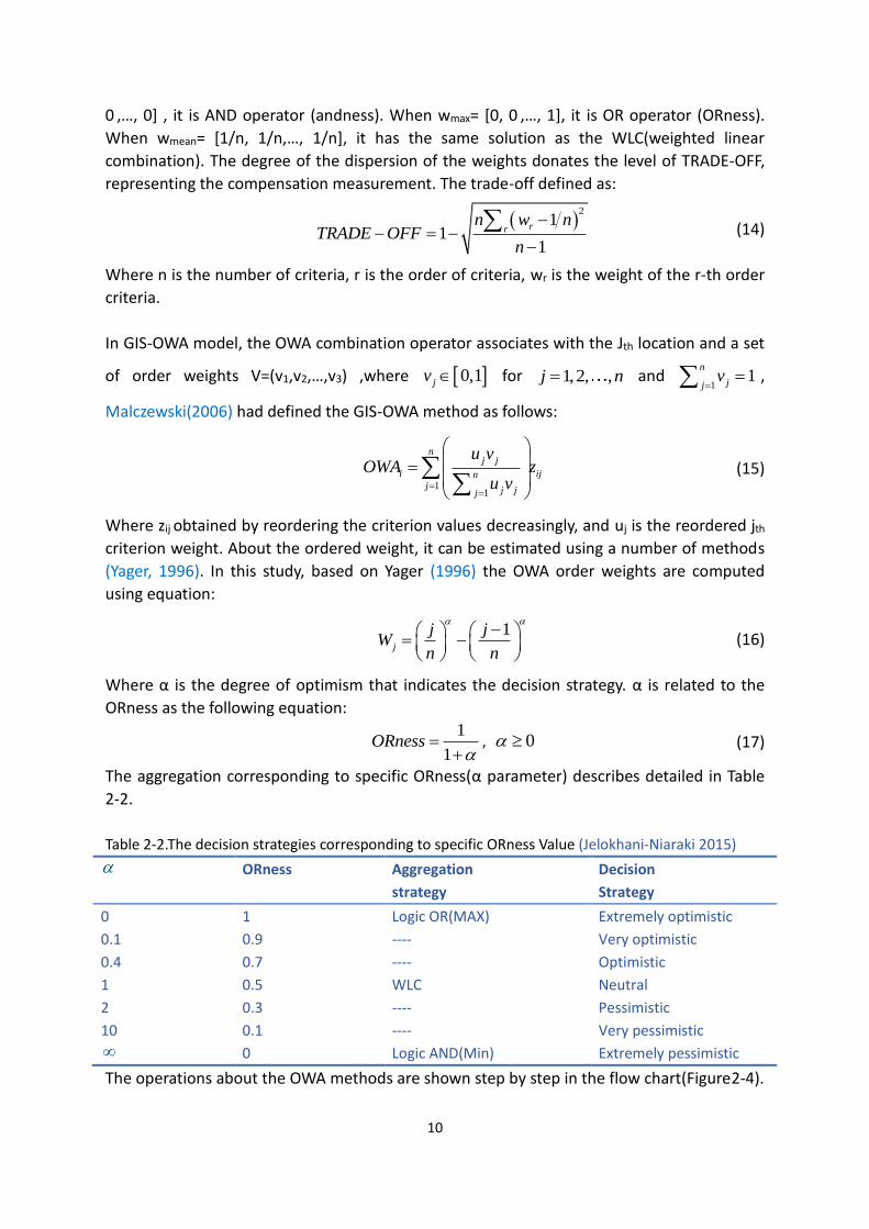
Actually, TOPSIS is a utility-based method that compares each alternative directly. It depends
on data in the evaluation matrices and weights (Cheng, S., Chan, C.W., Huang, G.H 2002). To
make group environment more manageable, many operations in the processing of TOPSIS
are scrutinized to be established. The operation inside TOPSIS includes: establish decision
matrix, decision matrix normalization, distance measure, aggregation operations. The
procedure of TOPSIS shown in flow chart(Figure 2-3).
Step 1: Construct performance matrix
Step 2: Normalize the decision matrix
Step 4: Detremine the PIS and NIS
Step 3: Assign a weight vector to the attribute set for the group
Step 5: Calculate distance PIS and NIS
Step 6: Calculate the relative closeness to the ideal solution for the group
Step 7: Rank the preference order
Figure 2-3.TOPSIS process flow chart
Step 1: performance matrix is constructed, create an evaluation matrix consisting of m
alternatives and n criteria, with the intersection of each alternative and criteria given as Xij ,
we therefore have a matrix (Xij)m×n .the structure of the matrix can be expressed as follows:
1 2
1 11 12 1
2 21 22 2
1 2
n
n
n
m m m mn
C C C
A x x x
A x x xD
A x x x
(3)
Step 2: normalize the decision matrix, using the normalization method:
2
1
, 1,2, , , 1,2, ,ij
ijm
iji
xr i m j n
x
(4)
Step 3: assign a weight vector to the attribute set for the group, construct the weighted
8
normalized decision matrix:
, 1,2, , , 1,2, ,ij j ijv w r i m j n (5)
Step 4: detremine the positive ideal and negative ideal solutions.
Positive ideal solution:
* * *
1 , , nA v v , * 'max( ), ;min( ),ij ijv v j J v j J (6)
Negative ideal solution:
' '
1 , , nA v v , ' 'min( ), ;max( ),ij ijv v j J v j J (7)
Step 5: calculate the separation measure for each alternative (calculate distance).The
separation from positive ideal alternative is:
* * 2
1
( )n
i ij j
j
S v v
, 1, ,i m (8)
The separation from negative ideal alternative is:
' 2
1
( )n
i ij j
j
S v v
, 1, ,i m (9)
Step 6: Calculate the relative closeness to the ideal solution Ci*:
* ' */ ( )i i i iC S S S , *0 1iC (10)
Step 7: rank the preference order, the larger the index value, the alternative performs better,
which also means the more Ci*value close to 1 the better.
2.2.3 Ordered Weighted averaging (OWA)
The ordered weighted averaging (OWA) is a class of multi-criteria aggregation or
combination operations developed by Yager (1988) which involves two set of weights:
criterion importance weights and ordered weights. The criterion weight Wj is assigned to the
jth criterion map for all locations to indicate the relative importance of the evaluation
criteria’s attribute according to the decision maker’s preferences. The ordered weights are
associated with the criterion values on the location-to-location basis. They are assigned to a
given ith location’s attribute value in decreasing order with no consideration from which
criterion map value comes. The ordered weights are central to the OWA combination
operators.
The OWA method has been developed in the context of fuzzy set theory (Yager,1988) in the
beginning. Eastman (1997) and Jiang implemented the OWA operations as a part of a
decision support module in GIS-IDRISI. Several authors offer the GIS-OWA approach to urban
planning and management (Asproth et al. 1999; Mendes 2000;Mendes and Motizuki 2001).
Fritz et, al. (2001) proposed that GIS-OWA operations could be used for wild-land perceptual
decision making. In most of the studies that mentioned before, the OWA method is test by
hypothetical decision scenarios. Jiang, H. and Eastman, J.R. (2000) remind that as a relatively
new research, OWA should be tested in a variety of decision making situations to make sure
9
how it may help decision maker in the real day life. The appeal of OWA is reordering and
changing criterion parameters, for that one can generate different solution maps and
scenarios. Different with the Boolean overlay AND operator which means the lowest risk
while the OR operator represents the highest risk in decision making, OWA method contains
a full spectrum of risk scenarios bounded between the AND and OR operators (Gorsevski,
P.V., Donevska, K.R, et al. 2012). Since the order weights are associated with the criterion
values on a location-to-location basis. The location’s attribute values are assigned to them in
decreasing order.
Yager (1988) proposed OWA as a parameterized family of combination operators. For a given
set of n criterion maps, the OWA function defined as follows, formally an OWA operator of
dimension n is a mapping F: Rn → R that has an associated collection of ordered weight W=
[w1, w2 ,…, wn] lying in the unit interval and summing to 1, given the set of attribute value
a1,a2,…,an, and the OWA equation is that:
1 2
1
, ,...,n
n j j
j
F a a a w b
(11)
Where, bj is the jth largest of the ai. For example, with a particular position of the attribute
values, the first order weight, w1, is assigned to the highest suitability attribute value; w2 is
assigned to the second highest suitability attribute value while wn is assigned to the lowest
suitability attribute value. The aggregation in OWA is achieved since the reordered weights
determined by the attribute values that are combined with the set of ordered weights. The
OWA operator provides a rich family of aggregation operators which are parameterized by
the weighting vector. Due to the OWA operator is a mean operator. It is bounded, monotonic,
symmetric, and idempotent.
Yager (1988) introduced two characterizing features associated with the weighting vector w
of OWA operator. The first is the attitudinal character (ORness), it is defined as:
1
1
1
n
j
j
A C W n j wn
, 0,1A C W (12)
In addition, A-C(max) is 1,A-C(med) is 0.5, A-C(min) is 0. Thus the A-C changes from 1 to 0 as
we go from Max to Min aggregation. The attitudinal character characterizes the similarity of
aggregation to OR operation, which OR defined as the Max. The second feature is the
dispersion. This defined as:
1
lnn
j j
j
H W w w
(13)
This value characterizes the degree of the arguments that being used.
There are several researches proposing that the position of order weights can be identified
based on the concepts of trade-off and risk. It can be achieved by varying the ordered
weights, and what’s in return, would generate a continuous aggregation procedure. The
ordered weights is W= [w1, w2 ,…, wn] ,where wn represents the ordered rank. When wmin= [1,
10
0 ,…, 0] , it is AND operator (andness). When wmax= [0, 0 ,…, 1], it is OR operator (ORness).
When wmean= [1/n, 1/n,…, 1/n], it has the same solution as the WLC(weighted linear
combination). The degree of the dispersion of the weights donates the level of TRADE-OFF,
representing the compensation measurement. The trade-off defined as:
21
11
rrn w n
TRADE OFFn
(14)
Where n is the number of criteria, r is the order of criteria, wr is the weight of the r-th order
criteria.
In GIS-OWA model, the OWA combination operator associates with the Jth location and a set
of order weights V=(v1,v2,…,v3) ,where 0,1jv for 1,2, ,j n and 1
1n
jjv
,
Malczewski(2006) had defined the GIS-OWA method as follows:
11
nj j
i ijnj j jj
u vOWA z
u v
(15)
Where zij obtained by reordering the criterion values decreasingly, and uj is the reordered jth
criterion weight. About the ordered weight, it can be estimated using a number of methods
(Yager, 1996). In this study, based on Yager (1996) the OWA order weights are computed
using equation:
1
j
j jW
n n
(16)
Where α is the degree of optimism that indicates the decision strategy. α is related to the
ORness as the following equation:
1
1ORness
, 0 (17)
The aggregation corresponding to specific ORness(α parameter) describes detailed in Table
2-2.
Table 2-2.The decision strategies corresponding to specific ORness Value (Jelokhani-Niaraki 2015)
ORness Aggregation
strategy
Decision
Strategy
0 1 Logic OR(MAX) Extremely optimistic
0.1 0.9 ---- Very optimistic
0.4
1
2
10
0.7
0.5
0.3
0.1
----
WLC
----
----
Optimistic
Neutral
Pessimistic
Very pessimistic
0 Logic AND(Min) Extremely pessimistic
The operations about the OWA methods are shown step by step in the flow chart(Figure2-4).

11
Step 1:Reordered attribute value
Step 2:Reordered criterion weights according to the attribute value
Step 3 :Calculate the Ordered weights
Step 4:Calculate OWA value
Figure 2-4.The OWA process flow chart
12
Chapter 3
3. Implementation
The aim of the implementation is to test the three methods: AHP, TOPSIS, OWA and compare
the results of these methods, by evaluating the susceptibility maps of these three models in
two case study areas : northwest Iran and mainland of Ecuador. One case study is visceral
leishmaniasis in north-western Iran; the other case study is dengue disease in Ecuador
(mainland). The study area was classified into seven categories of susceptibility: extremely
low, very low, low, medium, high, very high, and extremely high. Accordingly, the final
susceptibility map relies a lot on their controlling factors, the selection of the criteria factors
is important in this research. From some formal researches, both in social and physical
environment several factors strongly influence the VL disease, such as nomadic lifestyle,
climate condition, altitude of the area, etc.(Edrissian et al.,1988, Mirsamadi et al.,
Salahi-Moghaddam et al.).
For the visceral leishmaniasis in this research , 13 factors were defined, including river,
altitude, large river beds(RB),lakes and water reservoirs(LR), temperature,
precipitation(Rain),Irrigated farming and orchards(IF), dry farm(DF),rangelands with canopy
cover(RC),forest with canopy cover(FC),health center, nomads ,and settlement (ST) (Figure
3-1).As for environmental factors, people who live in high-temperature and
high-precipitation areas are more susceptible to VL disease; people who live in areas have
more IF and DF are more susceptible to VL disease; people live in area have less RC and FC
are more susceptible to VL disease. As for Socioeconomic factors, nomads and settlement
will increase people’s susceptibility to VL disease; people whose living area have more health
centers are more susceptible to VL disease. As for geographical factors, low elevation and
short distance to river will increase people’s susceptibility to VL disease; people who are
living more close to RB and LR are more susceptible to VL disease. For layers RB, LR, IF, DF, RC,
FC, ST, they are different classes in land cover layer, we extracted them from land cover
layers. Many factors were responsible for epidemic dengue disease during the past 20th
century, even though there still exits some non-understood ones (Gubler 1998), it still clear
that some geographical factors influence a lot on the spread of dengue. For dengue disease
in this case study, 4 factors were identified with the highest impact on the spread of disease
including temperature, precipitation, elevation, and distance to river (Figure 3-2).People
who are living in high temperature and precipitation area are more susceptible to dengue
disease; people who are living in low elevation and short distance to river area are more
susceptible to dengue disease. Experts have already decide the classification for the factor
layers.
13
Figure 3-1.Factors maps of VL disease in northwest Iran
Figure 3-2.Factors maps of dengue disease in Ecuador (mainland)

14
3.1 Study area
The first study area is inside Iran, mainly on two parts: Kalaybar( western part of East
Azerbaijian province;47°04´E, 38°29´N), Ahar(south of kalaybar; 47°02´E,38°52´N). The
second study area is Ecuador (mainland; 1°46´S, 78°12´W).
Figure 3-3.(1) Study area in East Azerbaijian,Iran; (2)Study area in the mainland of Ecuador.
3.2 Data source
The geographic data used in Iran comes from Iranian National Cartographic Center,
Meteorological Organization, Infectious and Tropical Diseases Research Center (ITDRC) of
MoH. The data used in Ecuador comes from the Ministry of health of Ecuador. The data for
Iran was collected from 2000 to 2008; the data for Ecuador was in 2015.The geographic data
are in the raster format. ArcMap 10.2.2 is applied to manipulate the spatial data. MATLAB is
applied to run the figures from the data in three models. The weights that used in the study
are acquired from experts.
3.3 VL disease In northwest Iran
Visceral leishmaniasis (VL), also known as black fever, is the most severe form in
leishmaniasis. This disease is the second-largest parasitic killer in the world endemic.
Leishmania infantum is the principal agent of human and canine VL in Iran (Mohebali et
al.,2002, 2004). The disease has been reported adventitiously in Iran with the southern and
north-western part being the primary epidemic. The physical and social environment of
northwest Iran have many factors associated with the Visceral leishmaniasis disease heavily
(Rajabi M,et al. 2014).
3.3.1 AHP results and map

15
In order to apply the AHP method described above, breaking of the complex unstructured
problem into its component factors is necessary. Geography, environment and social
economy are three mainly part that influence the spread of VL disease. So the influence
factors were classified into these three hierarchies. After the 13 factors being arranged in
hierarchic order, numerical factors will be assigned to them to make sure the judgment of
the relative importance of each factor is subjective. The judgements are then synthesized.
The factors compared against other factors is assigned a relative dominant value between 1
and 9 to the intersecting cell (Table 3-1).
Analyzing all these 13 factors in topography, meteorology and human environment, we
decide that the main criteria level in this AHP method contains three parts: Geographical
factors, Environmental factors, Socio-economic factors. In the sub criteria level , there is 4
factors under geographical factors( River, Altitude, Large river beds(RB),Lakes and water
reservoirs(LR)).For environmental factors, six factors including temperature,
precipitation(Rain),Irrigated farming and orchards(IF), dry farm(DF),rangelands with canopy
cover(RC),forest with canopy cover(FC) were considered. For Socio-economic factors, health
center, nomads and settlement (ST) were included. The main structure of the AHP criteria
level is drawn in Figure 3-4.
Influenced criterion factors
GeographicalFactors
(w=0.2299)
EnvironmentalFactors
(w=0.6480)
Socio-economicFactors
(w=0.1222)
River(w=0.1769)
Altitude(w=0.5371)
RB(w=0.1652)
Temperature(w=0.3297)
Precipitation(w=0.2585)
IF(w=0.1731)
DF(w=0.1182)
RC(w=0.0560)
FC(w=0.0645)
Health center(w=0.1916)
Nomads(w=0.7390)
Settlement(w=0.0694)
LR(w=0.1208)
Figure 3-4.APH hierarchy associated with VL
16
The weights in this research were gained from VL modeling expert. The weight values were
determined by AHP pairwise matrix for the datasets (Table 3-1). After that, CR value was
calculated to determine if the pairwise comparisons are consistent (this value should be less
than 0.1). One of the strengths of the AHP method is that it considers for inconsistent
relationships while at the same time, providing a CR as an indicator of the degree of
consistency or inconsistency (Forman and Selly 2001; Chen et al. 2009). In this study, the CR
results for the pairwise comparison matrix for these thirteen dataset layers were
0.0032(Table 3-2). It justifies the comparison of the characteristics were perfectly consistent.
And the relative weights were appropriate to be used in the VL susceptibility model.
Table 3-1.Pairwise comparison matrix, factor weights and consistency ratio of the data layers used
Factors 1 2 3 4 5 6 Eigen
values
Geographical
*River 1 0.1769
*Altitude 2 1 0.5371
*Large river beds(RB) 1 1/5 1 0.1652
*Lakes and water reservoirs(LR) 1 1/5 1/2 1 0.1208
Consistency ratio : 0.0627
Environmental
*Temperature 1 0.3297
*Precipitation(Rain) 1/2 1 0.2585
*Irrigated farming and orchards(IF) 1/4 1/4 1 0.1731
*Dry farm(DF) 1/3 1/3 1/3 1 0.1182
*Rangelands with canopy cover(RC) 1/4 1/4 1/4 1/3 1 0.0560
*Forest with canopy cover(FC) 1/3 1/3 1/4 1/3 1 1 0.0645
Consistency ratio : 0.0972
Socio-economical
*Health center 1 0.1916
*Nomads 6 1 0.7390
*Settlement(ST) 1/4 1/8 1 0.0694
Consistency ratio : -0.0952

17
Table 3-2.Pairwise comparison matrix for dataset layers of VL analysis
Factors 1 2 3 Eigen
values
Geographical 1 0.2299
Environmental 3 1 0.6480
Socio-economical 1/2 1/5 1 0.1222
Consistency ratio : 0.0032
There are 4 pairwise comparison matrices in all. One for the main criteria level shown in
Table 3-2, three for the sub-criteria level, the first sub-criteria is under geographic: river,
altitude, large river beds(RB), lakes and water reservoirs(LR), given in Table 3-1. The second
matrix for sub-criteria is under environment. The third matrix for sub-criteria is under
socio-economy. All the eigenvalues in each matrix should sum to be 1. Susceptibility
mapping using AHP model in this research was constructed using the following equation:
( )
( Pr )
( )
AHP AHPgeo AHP AHP AHP AHP
AHPenv AHP AHP AHP AHP AHP AHP
AHPsoc AHP AHP AHP
VL W River W Altitude W RB W LR W
W Temperature W ecipitation W IF W DF W RC W FC W
W Healthcenter W Nomads W Settlement W
(18)
The AHP method was implemented in ArcGIS. First, all layers were normalized. The
resolution is 100(m) ×100(m).Then under spatial analysis tool, raster calculator was chosen
to acquire the susceptibility mapping. Three sub level criterion maps were calculated:
geographical factor map, environmental factor map, socio-economic factor map. At last,
continue to choose the raster calculator to achieve final AHP map (Figure 3-5).

18
Figure 3-5.Susceptibility map of VL in northwest Iran by AHP
19
3.3.2 TOPSIS results and map
TOPSIS is a useful technique in dealing with multi-criteria problems. It helps decision makers
(DMs) to organize the problems into a logical structure to solve them in a more efficient way.
During this processing, analysis, comparisons, and alternatives rankings will be carried out.
In this research, the 13 criteria factors that mentioned in the AHP method were used.
According to the basic TOPSIS model, the 13 layers of different factors were normalized first.
Then they were combined into one layer with the cell size: 100(m) ×100(m). The attribute
table of the combined 13 factors layer included an 8145×13 table with the normalized value
of each reclassified cell. Considering the matrix form which is required in TOPSIS model,
transform the table value to a matrix shown as equation (19), the 13 columns represents the
13 evaluation goal factors; the number of the rows is 8145:
1 2 3 4 13
1,1 1,2 1,3 1,4 1,13
6,1 6,2 6,3 6,4 6,13
8145,1 8145,2 8145,3 8145,4 8145,13
f f f f f
x x x x x
x x x x xD
x x x x x
(19)
Data processing was performed using ArcGIS 10.2.2. Calculation of TOPSIS model was
performed using MATLAB. After combine all 13 factors layers into one, a matrix using for
TOPSIS model can be transformed from this layer’s attribute table. Chapter2.2.2 has
described the TOPSIS procedure, run this 8145×13 matrix within the TOPSIS algorithm in
MATLAB, the ideal closeness results were chosen to represent the TOPSIS final value.
Because this matrix has 8145 rows, the number of ideal closeness drawn from the TOPSIS
model is 8145(20 of them are selected randomly as a present Table 3-4).Then join the TOPSIS
value as a new column in the attribute table of the combined layer. The final susceptibility
map come from TOPSIS model was drawn by classified TOPSIS value in properties symbology
(Figure 3-6). The weights used in this model are listed in Table 3-3.
Table 3-3.Factors weights for TOPSIS model
Factors Weights
Settlement(ST)
Lakes and water reservoirs(LR)
0.1
0.05
Large river beds(RB) 0.05
Forest with canopy cover(FC) 0.01
Rangelands with canopy cover(RC)
Dry farm (DF)
Irrigated farming and orchards(IF)
Temperature
River
Precipitation(Rain)
0.01
0.04
0.04
0.15
0.05
0.1
20
Nomads
Health
Altitude
0.2
0.05
0.15
Table 3-4.The PIS NIS and ideal closeness value in TOPSIS model(pick 20 of 8145 figures as example)
ID Positive ideal distance Negative ideal distance Ideal closeness
2000 1.6158e-04 6.5688e-05 0.2890
2001 1.4879e-04 6.2943e-05 0.2973
2002 1.9096e-0.4 5.6275e-05 0.2276
2003
2004
2005
2006
2007
2008
2009
2010
2011
2012
2013
2014
2015
2016
2017
2018
2019
2020
1.9694e-0.4
1.8356e-0.4
1.7237e-0.4
1.7569e-0.4
1.8576e-0.4
1.4540e-0.4
1.6292e-0.4
1.6508e-0.4
2.0158e-0.4
1.8103e-0.4
1.5917e-0.4
1.3446e-0.4
1.4821e-0.4
1.6988e-0.4
1.8639e-0.4
1.7294e-0.4
1.3193e-0.4
1.6281e-0.4
5.0294e-05
5.0294e-05
6.4834e-05
5.5750e-05
6.0936e-05
7.6041e-05
8.3117e-05
6.7984e-05
4.2755e-05
5.0410e-05
6.7564e-05
9.3202e-05
6.9282e-05
5.0806e-05
5.7190e-05
5.8495e-05
7.8736e-05
6.7955e-05
0.2034
0.2567
0.2733
0.2409
0.2470
0.3434
0.3378
0.2917
0.1750
0.2178
0.2980
0.4094
0.3186
0.2302
0.2348
0.2527
0.3738
0.2945
21
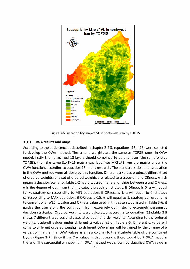
Figure 3-6.Susceptibility map of VL in northwest Iran by TOPSIS
3.3.3 OWA results and maps
According to the basic concept described in chapter 2.2.3, equations (15), (16) were selected
to develop the OWA method. The criteria weights are the same as TOPSIS ones. In OWA
model, firstly the normalized 13 layers should combined to be one layer (the same one as
TOPSIS), then the same 8145×13 matrix was load into MATLAB, run the matrix under the
OWA function, according to equation 15 in this research. The standardization and calculation
in the OWA method were all done by this function. Different α values produces different set
of ordered weights, and set of ordered weights are related to a trade-off and ORness, which
means a decision scenario. Table 2-2 had discussed the relationships between α and ORness.
α is the degree of optimism that indicates the decision strategy. If ORnees is 0, α will equal
to ∞, strategy corresponding to MIN operation; if ORness is 1, α will equal to 0, strategy
corresponding to MAX operation; if ORness is 0.5, α will equal to 1, strategy corresponding
to conventional WLC. α value and ORness value used in this case study listed in Table 3-6, it
guides the user along the continuum from extremely optimistic to extremely pessimistic
decision strategies. Ordered weights were calculated according to equation (16).Table 3-5
shows 7 different α values and associated optimal order weights. According to the ordered
weights, trade-off values under different α values list on Table 3-6. Different α value will
come to different ordered weights, so different OWA maps will be gained by the change of α
value. Joining the final OWA values as a new column to the attribute table of the combined
layers (Figure 3-7). Since it has 7 α values in this research, there would be 7 OWA maps in
the end. The susceptibility mapping in OWA method was shown by classified OWA value in

22
properties symbology (Figure 3-8 to Figure 3-14).
Criterion maps
Standardized
Weighted
Calculate OWA
Output Map
Criterion weights
Ordered weights
OWA operators
Figure 3-7.Flow chart of OWA
Table 3-5.Optimal order weights for selected values of the parameter α and the number of map
layers.
α
0 0.1 0.4 1 2 10 ∞
V1 0 0.7738 0.3584 0.0769 0.0059 7E-12 1
V2 0 0.0555 0.1145 0.0769 0.0178 7E-09 0
V3 0 0.0343 0.0833 0.0769 0.0296 4.2E-07 0
V4 0 0.0252 0.0678 0.0769 0.0414 7E-06 0
V5 0 0.0201 0.0583 0.0769 0.0533 6.3E-05 0
V6 0 0.0167 0.0516 0.0769 0.0651 0.0004 0
V7 0 0.0144 0.0467 0.0769 0.0769 0.0016 0
V8 0 0.0126 0.0428 0.0769 0.0888 0.0057 0
V9 0 0.0113 0.0397 0.0769 0.1006 0.0175 0
V10 0 0.0102 0.0372 0.0769 0.1124 0.0472 0
V11 0 0.0093 0.0350 0.0769 0.1243 0.1156 0
V12 0 0.0086 0.0331 0.0769 0.1361 0.2610 0
V13 1 0.0080 0.0315 0.0769 0.1479 0.5509 0
23
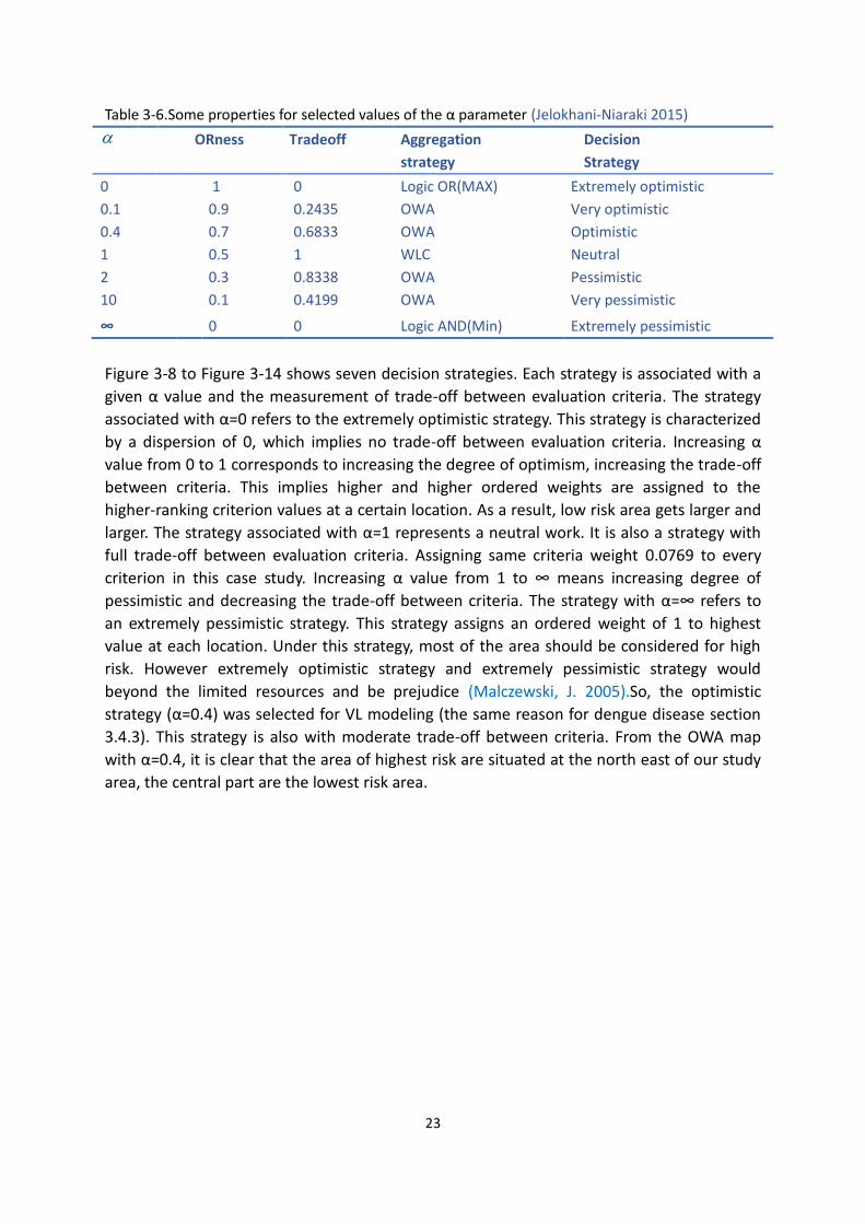
Table 3-6.Some properties for selected values of the α parameter (Jelokhani-Niaraki 2015)
ORness Tradeoff Aggregation
strategy
Decision
Strategy
0 1 0 Logic OR(MAX) Extremely optimistic
0.1 0.9 0.2435 OWA Very optimistic
0.4
1
2
10
0.7
0.5
0.3
0.1
0.6833
1
0.8338
0.4199
OWA
WLC
OWA
OWA
Optimistic
Neutral
Pessimistic
Very pessimistic
∞ 0 0 Logic AND(Min) Extremely pessimistic
Figure 3-8 to Figure 3-14 shows seven decision strategies. Each strategy is associated with a
given α value and the measurement of trade-off between evaluation criteria. The strategy
associated with α=0 refers to the extremely optimistic strategy. This strategy is characterized
by a dispersion of 0, which implies no trade-off between evaluation criteria. Increasing α
value from 0 to 1 corresponds to increasing the degree of optimism, increasing the trade-off
between criteria. This implies higher and higher ordered weights are assigned to the
higher-ranking criterion values at a certain location. As a result, low risk area gets larger and
larger. The strategy associated with α=1 represents a neutral work. It is also a strategy with
full trade-off between evaluation criteria. Assigning same criteria weight 0.0769 to every
criterion in this case study. Increasing α value from 1 to ∞ means increasing degree of
pessimistic and decreasing the trade-off between criteria. The strategy with α=∞ refers to
an extremely pessimistic strategy. This strategy assigns an ordered weight of 1 to highest
value at each location. Under this strategy, most of the area should be considered for high
risk. However extremely optimistic strategy and extremely pessimistic strategy would
beyond the limited resources and be prejudice (Malczewski, J. 2005).So, the optimistic
strategy (α=0.4) was selected for VL modeling (the same reason for dengue disease section
3.4.3). This strategy is also with moderate trade-off between criteria. From the OWA map
with α=0.4, it is clear that the area of highest risk are situated at the north east of our study
area, the central part are the lowest risk area.

24
Figure 3-8.Susceptibility map of VL in northwest Iran by OWA0 method
Figure 3-9. Susceptibility map of VL in northwest Iran by OWA0.1 method
25
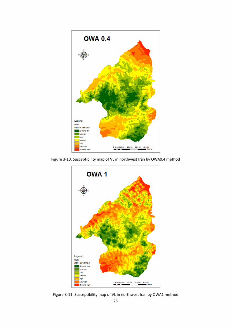
Figure 3-10. Susceptibility map of VL in northwest Iran by OWA0.4 method
Figure 3-11. Susceptibility map of VL in northwest Iran by OWA1 method
26
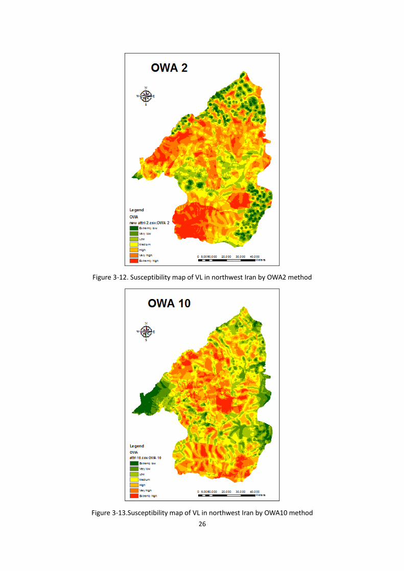
Figure 3-12. Susceptibility map of VL in northwest Iran by OWA2 method
Figure 3-13.Susceptibility map of VL in northwest Iran by OWA10 method

27
Figure 3-14.Susceptibility map of VL in northwest Iran by OWA∞ method
3.4 Dengue disease In Ecuador
Dengue fever (DF) is a global disease burden that infects an estimated 50-100 million
individuals in tropical and sub-tropical areas every year (Halstead 2007). It has rapidly
increased in geographic distribution, incidence in recent years. Through the bite mosquitoes,
the viruses are transmitted. Dengue is widely distributed in more than 100 countries in the
Americas, the Middle East, the Asia-Pacific region and Africa. The geographical limits
correspond approximately to a winter isotherm of 10°C, mostly between latitude 35°N and
35°S (World Health Organization 2009). Approximately 50 million epidemics occur each year.
In 2000, an outbreak of dengue in Ecuador included 22,937 cases reported to PAHO (Dick,
O.B., et al. 2012). It is now hyper-endemic in the coastal regions in Ecuador.
3.4.1 AHP results and map
According to the data in Ecuador, the case study of the dengue disease only had 4 factors
within one level, which are temperature, precipitation, elevation, and distance to river
respectively. The weight of each factors were gained from the questionnaire which we
collect suggestions from dengue modeling expert. The results of pairwise comparison are
shown in Table 3-7.
28
Table 3-7.Pairwise comparison matrix for dataset layers of Dengue analysis
Factors 1 2 3 4 Eigen
values
Temperature 1 0.3142
Precipitation 2 1 0.4172
Elevation 1/4 1/5 1 1/5 0.0649
Distance to river 1/3 1/2 5 1 0.2037
Consistency ratio : 0.0880
The susceptibility map using AHP model in this research was constructed using the following
equation:
Pr tanAHP AHP AHP AHP AHPDengue Temperature W ecipitatuon W Elevation W Dis ce W (20)
All the procedures for Ecuador data in AHP method are the same as VL disease in northwest
Iran. Final susceptibility map by AHP method is shown as Figure 3-15.
Figure 3-15.Susceptibility map of Dengue in Ecuador by AHP
3.4.2 TOPSIS results and map
29
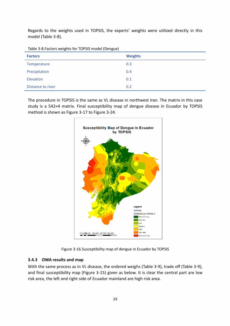
Regards to the weights used in TOPSIS, the experts’ weights were utilized directly in this
model (Table 3-8).
Table 3-8.Factors weights for TOPSIS model (Dengue)
Factors Weights
Temperature
Precipitation
0.3
0.4
Elevation 0.1
Distance to river 0.2
The procedure in TOPSIS is the same as VL disease in northwest Iran. The matrix in this case
study is a 542×4 matrix. Final susceptibility map of dengue disease in Ecuador by TOPSIS
method is shown as Figure 3-17 to Figure 3-24.
Figure 3-16.Susceptibility map of dengue in Ecuador by TOPSIS
3.4.3 OWA results and map
With the same process as in VL disease, the ordered weighs (Table 3-9), trade off (Table 3-9),
and final susceptibility map (Figure 3-15) given as below. It is clear the central part are low
risk area, the left and right side of Ecuador mainland are high risk area.

30
Table 3-9.Order weights for selected values of the parameter α and trade-off values
α
0 0.1 0.4 1 2 10 ∞
V1 0 0.8706 0.5743 0.2500 0.0625 9.5E-07 1
V2 0 0.0625 0.1835 0.2500 0.1875 0.0009 0
V3 0 0.0386 0.1334 0.2500 0.3125 0.055 0
V4 1 0.0284 0.1087 0.2500 0.4375 0.9437 0
Trade off 0 0.1721 0.5631 1.0000 0.6773 0.0736 0
Figure 3-17.Susceptibility map of dengue in Ecuador by OWA0

31
Figure 3-18. Susceptibility map of dengue in Ecuador by OWA0
Figure 3-19.Susceptibility map of dengue in Ecuador by OWA1

32
Figure 3-20. Susceptibility map of dengue in Ecuador by OWA2
Figure 3-21.Susceptibility map of dengue in Ecuador by OWA10

33
Figure 3-22. Susceptibility map of dengue in Ecuador by OWA ∞
Chapter 4
4. Results and Discussion
4.1 Validation of models used
4.1.1 VL disease in northwest Iran
Existing VL disease inventory points were used for the validation of these three models to
make comparison. 5 endemic points and 5 non-endemic points. Table 4-1 lists the figure of
area under category for each method; all the susceptibility categories for AHP, TOPSIS, OWA
(0.4), and WLC (OWA 1) are clearly listed by certain numbers in the table.
In OWA method, owing to different α parameter, a wide range of OWA solutions can be
generated. In this case study, exploring 7 scenarios of order weights by different parameter:
α= 0, 0.1, 0.4,1,2,10 and ∞ respectively (Section3.3.3). Increasing α value from 0 to ∞
corresponds to increasing ORness degree and trade-off between evaluation criteria. The
criterion substitutability expressed by the trade-off value, it illustrates the degree of the
performance. Comparing all of 7 corresponding maps in Figure 3-8 to Figure 3-14, along with
decreasing the ORness (increasing trade-off), the VL disease high risk areas get smaller and
smaller. It has already mentioned in Section3.3.3, α equals 1 represents WLC, this strategy
characterized by full trade-off and 0.5 ORness. Considering all the trade-off values of
different α value, as it mentioned in section3.3.3, OWA0.4 were chosen to represent the
34
OWA method, because OWA 1 also represents WLC, we also choose this one.
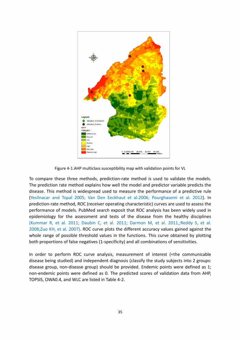
For instance, AHP method (Figure 4-1) was interpreted as follows(Table 4-1): (i) the sum of
the extremely high, very high and high susceptibility zones account for 40.65%
(4.40%+16.87%+19.38%) of the entire study area, contained 40% non-endemic validation
points and 100% endemic validation points . (ii) the moderate susceptibility zones account
for 14.32% of the study area and no endemic and non-endemic points in this category. (iii)
the sum of extremely low, very low and low susceptibility zones occupied 45.03%
(8.57%+20.24%+16.22%), contained no endemic validation and 60% of the non-endemic
points.
Table 4-1.Areas under category (%) for each method
Method
Susceptibility category (%)
Extremely
low Very low Low Medium High Very high
Extremely
high
AHP 8.57% 20.24% 16.22% 14.32% 19.38% 16.87% 4.40%
TOPSIS 10.16% 23.77% 26.28% 20.70% 11.44% 5.07% 2.58%
OWA (0.4) 10.35% 16.25% 21.55% 23.42% 18.90% 7.75% 1.78%
WLC(OWA1) 4.00% 11.25% 17.92% 22.46% 21.97% 17.38% 5.02%
Figure 4-1 shows the susceptibility map from AHP methods and add 10 validation points in
this map. The black points are endemic, and green points are non-endemic. The predictions
confirm to the calculation of the model, except 2 validation points (non-endemic) in the
southwest area.
35
Figure 4-1.AHP multiclass susceptibility map with validation points for VL
To compare these three methods, prediction-rate method is used to validate the models.
The prediction rate method explains how well the model and predictor variable predicts the
disease. This method is widespread used to measure the performance of a predictive rule
(Yesilnacar and Topal 2005; Van Den Eeckhaut et al.2006; Pourghasemi et al. 2012). In
prediction-rate method, ROC (receiver operating characteristic) curves are used to assess the
performance of models. PubMed search exposit that ROC analysis has been widely used in
epidemiology for the assessment and tests of the disease from the healthy disciplines
(Kummar R, et al. 2011; Daubin C, et al. 2011; Darmon M, et al. 2011,;Reddy S, et al.
2008;Zuo KH, et al. 2007). ROC curve plots the different accuracy values gained against the
whole range of possible threshold values in the functions. This curve obtained by plotting
both proportions of false negatives (1-specificity) and all combinations of sensitivities.
In order to perform ROC curve analysis, measurement of interest (=the communicable
disease being studied) and independent diagnosis (classify the study subjects into 2 groups:
disease group, non-disease group) should be provided. Endemic points were defined as 1;
non-endemic points were defined as 0. The predicted scores of validation data from AHP,
TOPSIS, OWA0.4, and WLC are listed in Table 4-2.

36
Table 4-2.Validation data used for AHP, TOPSIS, OWA 0.4, WLC
State AHP TOPSIS OWA 0.4 WLC
0 3.7795 0.6424 0.0581 -0.2506
0 3.8998 0.5692 0.1156 -0.2000
0 2.7465 0.2282 0.0386 -0.2471
0 2.9185 0.1916 0.1498 -0.1394
0 2.7263 0.2060 0.1977 -0.1131
1 3.8992 0.3768 0.1320 -0.1849
1 3.6063 0.2624 0.1165 -0.1702
1 3.7959 0.2803 0.1485 -0.1597
1 3.6782 0.3410 0.1422 -0.1645
1 4.4530 0.7433 0.1563 -0.1481
The area under ROC curve (AUC) which as a one-dimensional index, were calculate to
measure the classification performance. AUC value varies from 0 to 1.The maximum value 1
means that the diagnostic test is perfect. 0.5 represents a worthless test. 0 indicates the
result is completely wrong. AUC value from 0.5 to 1 means a good fit, while value below 0.5
presents a random fit (Swets 1988).
Figure 4-2 shows the ROC curves of the three models for VL disease in northwest Iran. Table
4-3 lists the AUC values of the three models.
Figure 4-2.The ROC curves for AHP, TOPSIS, OWA 0.4, WLC

37
Table 4-3.AUC values of TOPSIS,AHP, OWA 0.4, WLC for VL disease in northwest Iran
Test Result Variable(s) AUC
TOPSIS 0.680
AHP 0.760
OWA 0.4 0.640
WLC 0.600
Consider ROC curves of these three models together; it is obvious that their overall
performance of the curves is close to each other. For more strict accuracy control, the
comparison of AUC value is necessary. As a result, AHP (0.760) has higher prediction
performance than TOPSIS (0.680), OWA 0.4(0.640) and WLC (0.600).From this plot, it can be
concluded that AHP is the best one.
As to reason, it might be mainly caused by the factors: the number of the factors, the
processing mode of the factors weights. For the number, too many factors were analyzed in
this disease (some comparison will be made in 4.1.2). For the procedure, in AHP method,
pairwise comparison was used to balance the weights from the expert, which made the
factors weights more objective. TOPSIS and OWA invest the expert weights directly from the
questionnaire. That make the weights depends more on experts’ own opinion. It is also one
shortcoming of knowledge-driven techniques.
4.1.2 Dengue disease in Ecuador
For dengue disease in Ecuador, validation areas were added to test the models, 4
non-endemic areas and 6 endemic areas were selected for the validation. The results are
listed in Table 4-4. For OWA method results, comparing all of 7 corresponding maps in Figure
3-11, along with decreasing the ORness (increasing trade-off), the dengue disease high risk
areas get larger and larger. Take AHP model as an example, it was interpreted as follows: (i)
the sum of extremely high, very high and high susceptibility zones account for 27.82%
(1.50%+8.11%+18.21%) of the entire study area. (ii) the moderate susceptibility zones
account for 23.31% of the entire study area. (iii) the sum of extremely low, very low and low
susceptibility zones account for 48.87% (7.00%+18.38%+23.49%).
Table 4-4.Areas under category (%) for each method
Susceptibility category (%)
Extremely
low
Very low Low Medium High Very high Extremely
high
AHP 7.00% 18.38% 23.49% 23.31% 18.21% 8.11% 1.50%
TOPSIS 16.23% 17.66% 15.49% 16.47% 20.30% 11.63% 2.23%
OWA (0.4) 6.10% 21.82% 2.61% 5.55% 8.54% 18.08% 37.31%
WLC(OWA1) 14.19% 9.35% 7.68% 4.74% 3.85% 26.02% 34.17%

38
Figure 4-3 shows the susceptibility map resulted from AHP method and add the validation
areas in this map. 10 areas were selected from east west south north and middle part of
Ecuador. Due to the lack of data in the east of Ecuador, so the northeast part was selected to
represent that area. The darker the red color is, the more risk of dengue export in that area
has. The same to VL disease, endemic areas were given state as 1, non-endemic area were
given state as 0. The predicted scores of validation data from AHP, TOPSIS, OWA0.4, and WLC
are listed in Table 4-5.Table 4-6 lists the AUC values of these four models.
Figure 4-3.AHP multiclass susceptibility map with validation areas for dengue
Table 4-5.Validation data used for AHP, TOPSIS, OWA 0.4, WLC
State AHP TOPSIS OWA 0.4 WLC
1 2.3598 0.1985 0.7425 0.3000
1 3.0814 0.2706 0.7586 0.2449
1 3.5537 0.3723 0.4934 0.1567
1 2.6740 0.2494 0.7715 0.3153
1 3.0716 0.2341 0.6069 0.0728
1 1.7775 0.0337 0.6761 0.3464
0 1.8321 0.0804 0.7273 0.2449
0 1.6482 0.0872 0.1036 -0.3618
0 2.2027 0.1644 0.1292 -0.1225
0 1.6482 0.0826 0.1213 -0.3548
39
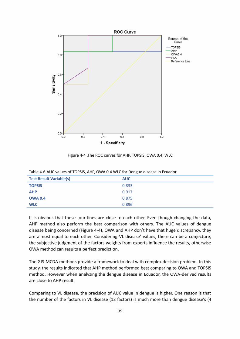
Figure 4-4 .The ROC curves for AHP, TOPSIS, OWA 0.4, WLC
Table 4-6.AUC values of TOPSIS, AHP, OWA 0.4 WLC for Dengue disease in Ecuador
Test Result Variable(s) AUC
TOPSIS 0.833
AHP 0.917
OWA 0.4 0.875
WLC 0.896
It is obvious that these four lines are close to each other. Even though changing the data,
AHP method also perform the best comparison with others. The AUC values of dengue
disease being concerned (Figure 4-4), OWA and AHP don’t have that huge discrepancy, they
are almost equal to each other. Considering VL disease’ values, there can be a conjecture,
the subjective judgment of the factors weights from experts influence the results, otherwise
OWA method can results a perfect prediction.
The GIS-MCDA methods provide a framework to deal with complex decision problem. In this
study, the results indicated that AHP method performed best comparing to OWA and TOPSIS
method. However when analyzing the dengue disease in Ecuador, the OWA-derived results
are close to AHP result.
Comparing to VL disease, the precision of AUC value in dengue is higher. One reason is that
the number of the factors in VL disease (13 factors) is much more than dengue disease’s (4
40
factors). Because the huge amount of criteria and heterogeneity of data, results’ uncertainty
remains unclear. Even some small changes in weights may have a significant impact on the
final results. Another reason is that the study area for VL disease is smaller than the study
area for dengue disease; in general, enough data will provide a high accuracy test.
4.2 limitation
As mentioned above, within the three models, the best results can be gained by using AHP
methods. One reason of these may cause by the weights given by experts. It is also one of
the intrinsic deficiencies of knowledge driven technology, different experts will probably give
different weights based on their own opinion.
From the AUC value of these models in VL disease and dengue disease, it can also be
conclude that the lack of data influences the validation of the models. In the other words,
for VL disease in Iran, the study area is only the northwest of Iran, for dengue disease the
data tested in the models were the all Ecuador (mainland), but the study area in Iran is
somewhat not large enough. That’s why the test results in Ecuador is conspicuous than that
in Iran.
41
Chapter 5
5. Conclusion
This thesis has focused on comparing Multi-criteria decision Analysis methods for
susceptibility mapping in spatial communicable disease study. Related terminologies
(literature review) are first introduced in Chapter 2, which contains the processing of the
AHP, TOPSIS and OWA methods. Followed by the case study chapter, two case studies are
presented to illustrate the methods: VL disease in northwest Iran, dengue disease in Ecuador
(mainland). Finally the results (susceptibility maps) from these three methods are compared
by the AUC values from ROC curves.
When using GIS-MCDA methods, it is evident that each method has advantages and
limitations (Kritikos and Davies 2011).Based on this idea, in this study, the accuracy of the
three GIS-MCDA methods had been compared. TOPSIS and OWA method were implemented
in the same way: the ideal closeness values for TOPSIS and OWA values under different α
values were calculate in MATLAB first, then join the value in ArcGIS to obtain the
susceptibility maps of the disease. AHP method used the spatial analysis tools: raster
calculator to combine all the factor layers to gain the susceptibility map of the disease.
These investigations expose the capabilities of the three methods for susceptibility mapping
in spatial communicable disease study. The results indicate that, in this particular application,
the AHP method obtained the best predictive accuracy. However, it still be found if the data
is enough OWA method almost have the same predictive accuracy as AHP. Analyzing the
results from both VL disease and dengue disease, although TOPSIS performed worst in these
three methods, it still had high AUC values. In conclusion, AHP method has the most concise
procedures and highest accuracy in the prediction of infectious disease.
The limitation of this study can be concluded in two aspects: model limitation and data
limitation. With respects to model limitation, the numbers of factors influence the final
results, complicated factors in VL disease generate all the AUC values in these three methods
lower than that in dengue disease. For data limitation, one is the restriction of experts’
weights. Another data limitation is the lack of validation data, for VL disease validation we
only have 10 points. For dengue disease validation, even though the patient and population
rate area created as the validation area, but the deficiency of patients data in some regions
still confine the precision of validation.
For future study, temporal prediction can be added to draw the risk prediction maps.
Different with other risk map, no time factors is associated with a susceptibility map. All the
prediction in this study is in a non-specified time span. If enough data provided,
spatial-temporal prediction can be made from maps, which will provide more accurate
prediction of the communicable disease.

42
Reference
Asproth, V., Holmberg S .and Håkansson A.(1999) Decision support for spatial planning and
management of human settlements, Advances in support systems research Vol V:
Decision support methodology for human systems management and its applications in
economics and commerce.
Best, N., Richardson, S, Thomson, A.,(2005) A comparison of Bayesian spatial models for
disease mapping . Statistical Methods in medical Research,14(1),pp.35-59.
Belenson, S.M.,Kapur, K.C., An algorithm for solving multicriterion linear programming
problems with examples, Operational Research Quarterly,pp. 65–77.
Boroushaki, S., Malczewski, J.(2008) Implementing an extension of the analytical hierarchy
process using ordered weighted averaging operators with fuzzy quantifiers in ArcGIS.
Computers & Geosciences 34.4, pp.399–410.
Chen, Y., Khan, S. and Paydar, Z.(2010) To retire or expand? A fuzzy GIS-based spatial
multi-criteria evaluation framework for irrigated agriculture. Irrig Drain 59(2),pp.174–
188.
Cheng, S., Chan, C.W., Huang, G.H.(2002) Using multiple criteria decision analysis for
supporting decision of solid waste management, Journal of Environmental Science and
Health, Part A,37 (6),pp.975–990.
Daubin, C., Quentin, C., Allouche, S., et al.(2011)Serum neuron-specific enolase as predictor
of outcomes in comatose cardiac arrest survivor: a prospective cohort study. BMC
Cardiovasc Disord.11(1),p.1.
Darmon, M., Vincent, F., Dellamonica, J.,et al.(2011) Diagnostic performance of fractional
excretion of urea in the evaluation of critically III patients with acute kidney injury: a
multicenter cohort study. Crit Care .15(4),p.R178.
Dick, O. B., San Martin, J. L., Montoya R.H., et al.(2012) The history of Dengue Outbreak in
the Americas. The American Society of Tropical Medicine and Hygiene,87(4),
pp.584-593.
Eastman, J.R.(1997) IDRISI para Windows:Version 2.0,Enero 1997.Tutorial Exercises Clark
University.
Edrissian, G., Hafizi, A., Afshar, A.,et al.(1988) An endemic focus of visceral leishmaniasis in
Meshkin-Shahr, east Azerbaijan province, north-west part of Iran and IFA serological
survey of the disease in this area. Bulletin de la societé de pathologie exotique et de ses
filiales, 81(2), pp.238-248.
Feizizadeh, B., Blaschke, T., Nazmfar, H. et al. (2013) Landslide susceptibility mapping for the
Urmia Lake basin, Iran: a multi-criteria evaluation approach using GIS. Int J Environ Res,
7(2),pp.319-336.
Forman, E.H., Selly, M.A.(2001) Decision by objective, how to convince others that you are
right. World Scientific Publishing Co. Pte. Ltd, Singapore
Fritz, S., See, L. and Carver, S.(2001) A fuzzy modelling approach to wild land mapping in
Scotland. Innovations in GIS, 7,pp.219-230.
Gorsevski, P.V., Jankowski, P., Gessler PE.(2006) Heuristic approach for mapping landslide
hazard by integrating fuzzy logic with analytic hierarchy process. Control and
Cybernetics.35(1),p.121.
43
Gorsevski, P.V., Donevska, K.R., Mitrovski, C.D. et al.(2012) Integrating multi-criteria
evaluation techniques with geographic information systems for landfill site selection: a
case study using ordered weighted average. Waste Management 32(2),pp.287–296.
Greene, R., Devillers, R., Luther, J.E., et al.(2011). GIS-Based Multiple-Criteria Decision
Analysis. Geography Compass, 5(6),pp.412–432.
Gubler, D.J.(1998) Dengue and dengue hemorrhagic fever. Clinical microbiology
reviews, 11(3), pp.480-496.
Halstead, S.B. (2007). Dengue. The Lancet, 370(9599), pp.1644-1652.
Hwang, C.L., Yoon, K.(1981) Multiple Attribute Decision Making, Springer-Verlag, Berlin.
Jacquez, G.M.(2000) Spatial analysis in epidemiology: Nascent science or a failure of
GIS? Journal of Geographical Systems,2(1), pp.91-97.
Jankowski, P. and Richard, L.(1994) Integration of GIS-based suitability analysis and
multicriteria evaluation in a spatial decision support system for route
selection. Environment and Planning B: Planning and Design, 21(3), pp.323-340.
Jelokhani-Niaraki, M. and Malczewski, J.(2015). A group multicriteria spatial decision support
system for parking site selection problem: A case study. Land Use Policy, 42,
pp.492-508.
Jiang, H. Eastman, J.R. (2000) Application of fuzzy measures in multi-criteria evaluation in
GIS. Int J Geogr Inform Sci 14(2), pp.173–184.
Krieger, N., (2003)Place, Space, and Health: GIS and Epidemiology. Epidemiology,
14(4),pp.384-385.
Kritikos, T.R. and Davies T.R.(2011) GIS-based Multi-Criteria Decision Analysis for landslide
susceptibility mapping at northern Evia, Greece[GIS-basierte multikriterielle
Entscheidungsanalysen zur Kartierung von Massenverlagerungspotenzialen im
nördlichen Evia, Griechenland.].Zeitschrift der Deutschen Gesellschaft für
Geowissenschaften, 162(4), pp.421-434.
Kummar, R., Indrayan, A.,(2011) Receiver operating characteristic (ROC) curve for medical
researchers. Indian Pediatr,48(4),pp.277–287.
Lai, Y.J., Liu, T.Y. and Hwang, C.L.(1994) Topsis for MODM. European Journal of Operational
Research,76(3), pp.486-500.
Linkov, I., Satterstrom, F.K., Steevens, J., et al. (2007) Multi-criteria decision analysis and
environmental risk assessment for nanomaterials. Journal of Nanoparticle
Research, 9(4), pp.543-554.
Malczewski, J. (1999) GIS and multicriteria decision analysis. John Wiley& Sons,Toronto.
Malczewski, J.(2005)Integrating multicriteria analysis and geographic information systems:
the ordered weighted averaging (OWA) approach. International Journal of
Environmental Technology and Management, 6(1-2), pp.7-19.
Malczewski, J. (2006) GIS-based multicriteria decision analysis: a survey of the literature. Int
J Geogr Inform Sci, 20(7), pp.703–726.
Marinoni, O. (2004) Implementation of the analytical hierarchy process with VBA in
ArcGIS. Computers & Geosciences, 30(6), pp.637-646.
Melnick, A.L., Fleming, D.W.(1999) Modern Geographic Information Systems-Promise and
Pitfalls. J Public Health Manag Pract,5(2), pp.viii-hyhen.

44
Mendes, J.F.(2000)Decision strategy spectrum for the evaluation of quality of life in cities.
Planning for a Better Quality of Life in Cities, National University of Singapore,Singapore,
pp.35-53.
Mendes, J.F., Motizuki ,W.S.(2001) Urban quality of life evaluation scenarios: The case of
Sao Carlos in Brazil. CTBUH review, 1(2), pp.13-23.
McMichael, A.J. (2013). Globalization, climate change, and human health. New England
Journal of Medicine, 368(14), pp.1335-1343.
Mirsamadi, N., Mohebali, M., ATARI, M.,et al.(2003)Serological survey of Visceral
leishmaniasis (kala-azar) in Azarshahr, Azarbaijan province, northwest of Iran.
Mohebali, M., Motazedian, M.H., Parsa F., et al.(2002). Identification of Leishmania species
from different parts of Iran using a random amplified polymorphic DNA in human,
animal reservoirs and vectors. Med J Islamic Republic Iran ,15,pp.243-246.
Mohebali, M., Javadian, E., Yaghoobi Ershadi M.R.,et al.(2004) Characterization of
Leishmania infection in rodents from endemic areas of the Islamic Republic of Iran. East
Mediterr Health J,10, pp.591-599.
Pourghasemi, H.R., Pradhan, B. and Gokceoglu, C.(2012) Application of fuzzy logic and
analytical hierarchy process (AHP) to landslide susceptibility mapping at Haraz
watershed, Iran. Natural Hazards,63(2), pp.965-996.
Rajabi M, Mansourian Ali, Pilesjö P et al.(2014) Environmental modelling of visceral
leishmaniasis by susceptibility-mapping using neural networks: A case study in
north-western Iran. Geospatial Health, 9(1),pp.179-191.
Reddy, S., Dutta, S., Narang, A.,(2008) Evaluation of lactate dehydrogenase, creatine kinase
and hepatic enzymes for retrospective diagnosis of perinatal asphyxia among sick
neonates. Indian Pediatr. 45(2),p.144.
Saaty, T.L., (1977) A scaling method for priorities in hierarchical structures. J Math Psychol
15(3),pp.234-281
Saaty, T.L.(1980) The Analytic Hierarchy Process: Planning, Priority Setting, Resource
Allocation. New York: McGraw.
Saaty, T.L.(2008) Decision making with the analytic hierarchy process. International journal of
services sciences, 1(1), pp.83-98.
Salahi-Moghaddam Abdoreza, A., Mohebali Mehdi, M., Ali, M., et al.(2010) Ecological study
and risk mapping of visceral leishmaniasis in an endemic area of Iran based on a
geographical information systems approach. Geospatial health.
Swets, J.A.(1988) Measuring the accuracy of diagnostic systems. Science,240(4857),pp.1285–
1293.
Van Den Eeckhaut, M., Vanwalleghem, T., Poesen, J., et al. (2006) Prediction of landslide
susceptibility using rare events logistic regression: a case-study in the Flemish Ardennes
(Belgium). Geomorphology, 76(3), pp.392-410.
World Health Organization, Special Programme for Research, Training in Tropical Diseases,
World Health Organization. Department of Control of Neglected Tropical Diseases,
World Health Organization. Epidemic and Pandemic Alert, 2009. Dengue: guidelines for
diagnosis, treatment, prevention and control. World Health Organization.
Yager, R.R.(1988) On ordered weighted averaging aggregation operators in multi-criteria
decision making, IEEE Trans. Syst., Man, Cybern,18(1), pp.183–190.
45
Yager, R.R.(1996) Quantifier guided aggregation using OWA operators. International Journal
of Intelligent Systems, 11(1), pp.49-73.
Yesilnacar, E. and Topal, T. (2005) Landslide susceptibility mapping: a comparison of logistic
regression and neural networks methods in a medium scale study, Hendek region
(Turkey). Engineering Geology, 79(3), pp.251-266.
Zou, K.H., O’Malley, A.J., Mauri, L.(2007) Receiver-operating characteristic analysis for
evaluation diagnostic tests and predictive models. Circulation, 115(5),pp.654–657.
Zhu, L., Huang, J.F.(2006) GIS-based logistic regression method for landslide susceptibility
mapping in regional scale. J Zhejiang Univ Sci A,7(12),pp.2007–2012
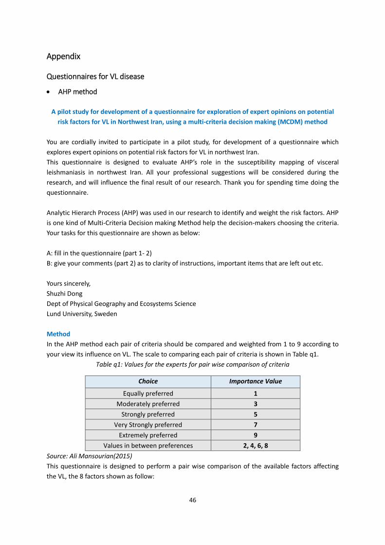
46
Appendix
Questionnaires for VL disease
AHP method
A pilot study for development of a questionnaire for exploration of expert opinions on potential
risk factors for VL in Northwest Iran, using a multi-criteria decision making (MCDM) method
You are cordially invited to participate in a pilot study, for development of a questionnaire which
explores expert opinions on potential risk factors for VL in northwest Iran.
This questionnaire is designed to evaluate AHP’s role in the susceptibility mapping of visceral
leishmaniasis in northwest Iran. All your professional suggestions will be considered during the
research, and will influence the final result of our research. Thank you for spending time doing the
questionnaire.
Analytic Hierarch Process (AHP) was used in our research to identify and weight the risk factors. AHP
is one kind of Multi-Criteria Decision making Method help the decision-makers choosing the criteria.
Your tasks for this questionnaire are shown as below:
A: fill in the questionnaire (part 1- 2)
B: give your comments (part 2) as to clarity of instructions, important items that are left out etc.
Yours sincerely,
Shuzhi Dong
Dept of Physical Geography and Ecosystems Science
Lund University, Sweden
Method
In the AHP method each pair of criteria should be compared and weighted from 1 to 9 according to
your view its influence on VL. The scale to comparing each pair of criteria is shown in Table q1.
Table q1: Values for the experts for pair wise comparison of criteria
Choice Importance Value
Equally preferred 1
Moderately preferred 3
Strongly preferred 5
Very Strongly preferred 7
Extremely preferred 9
Values in between preferences 2, 4, 6, 8
Source: Ali Mansourian(2015)
This questionnaire is designed to perform a pair wise comparison of the available factors affecting
the VL, the 8 factors shown as follow:
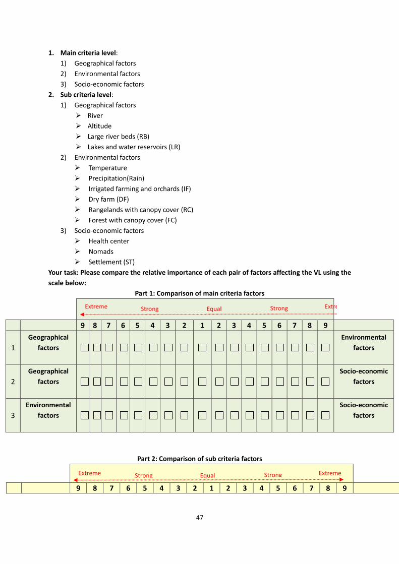
47
1. Main criteria level:
1) Geographical factors
2) Environmental factors
3) Socio-economic factors
2. Sub criteria level:
1) Geographical factors
River
Altitude
Large river beds (RB)
Lakes and water reservoirs (LR)
2) Environmental factors
Temperature
Precipitation(Rain)
Irrigated farming and orchards (IF)
Dry farm (DF)
Rangelands with canopy cover (RC)
Forest with canopy cover (FC)
3) Socio-economic factors
Health center
Nomads
Settlement (ST)
Your task: Please compare the relative importance of each pair of factors affecting the VL using the
scale below:
Part 1: Comparison of main criteria factors
9 8 7 6 5 4 3 2 1 2 3 4 5 6 7 8 9
1
Geographical
factors
Environmental
factors
2
Geographical
factors
Socio-economic
factors
3
Environmental
factors
Socio-economic
factors
Part 2: Comparison of sub criteria factors
9 8 7 6 5 4 3 2 1 2 3 4 5 6 7 8 9
Equal Extreme Extreme Strong Strong

48
9 8 7 6 5 4 3 2 1 2 3 4 5 6 7 8 9
1 River Altitude
2 River RB
3 River LR
4 Altitude RB
5 Altitude LR
6 RB LR
Part 3: Which statement do you agree with regards to each factor?
Environment factors
Temperature
People who are living in the high-temperature areas are more susceptible to VL
People who are living in the low-temperature areas are more susceptible to VL
Precipitation
People who are living in the high-precipitation areas are more susceptible to VL
People who are living in the low-precipitation areas are more susceptible to VL
IF
People who are living in the areas have more Irrigated farming and orchards are more susceptible to
VL
People who are living in the areas have less Irrigated farming and orchards are more susceptible to
VL
DF
People who are living in the areas have more dry farm are more susceptible to VL
People who are living in the areas have less dry farm are more susceptible to VL
RC
People who are living in the areas have more rangelands with canopy cover are more susceptible to
VL
People who are living in the areas have less rangelands with canopy cover are more susceptible to VL
FC
People who are living in the areas have more forest with canopy cover are more susceptible to VL
Equal Extreme Extreme Strong Strong
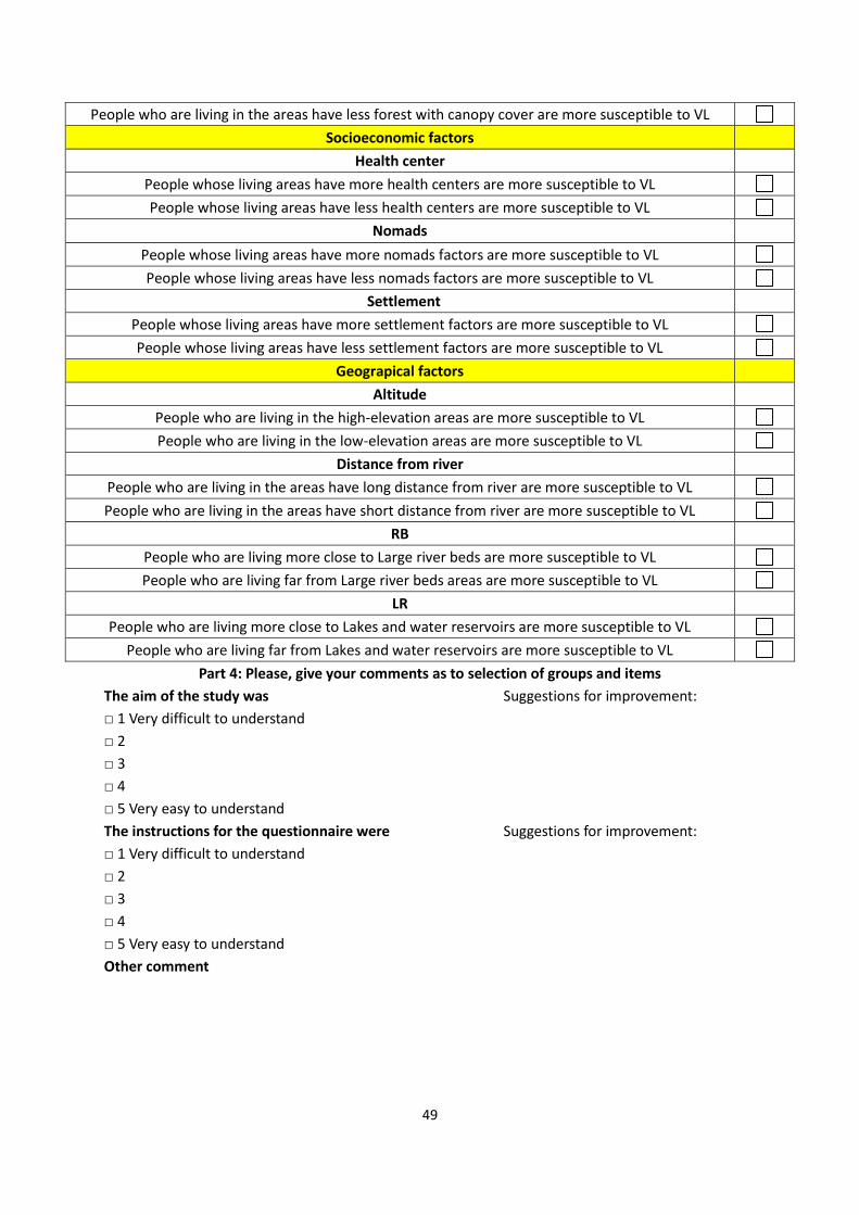
49
People who are living in the areas have less forest with canopy cover are more susceptible to VL
Socioeconomic factors
Health center
People whose living areas have more health centers are more susceptible to VL
People whose living areas have less health centers are more susceptible to VL
Nomads
People whose living areas have more nomads factors are more susceptible to VL
People whose living areas have less nomads factors are more susceptible to VL
Settlement
People whose living areas have more settlement factors are more susceptible to VL
People whose living areas have less settlement factors are more susceptible to VL
Geograpical factors
Altitude
People who are living in the high-elevation areas are more susceptible to VL
People who are living in the low-elevation areas are more susceptible to VL
Distance from river
People who are living in the areas have long distance from river are more susceptible to VL
People who are living in the areas have short distance from river are more susceptible to VL
RB
People who are living more close to Large river beds are more susceptible to VL
People who are living far from Large river beds areas are more susceptible to VL
LR
People who are living more close to Lakes and water reservoirs are more susceptible to VL
People who are living far from Lakes and water reservoirs are more susceptible to VL
Part 4: Please, give your comments as to selection of groups and items
The aim of the study was Suggestions for improvement:
□ 1 Very difficult to understand
□ 2
□ 3
□ 4
□ 5 Very easy to understand
The instructions for the questionnaire were Suggestions for improvement:
□ 1 Very difficult to understand
□ 2
□ 3
□ 4
□ 5 Very easy to understand
Other comment

50
TOPSIS and OWA method
A questionnaire for Multi Criteria Decision Making for studies of VL with the help of TOPSIS and
OWA Process
You are cordially invited to participate in a study, for development of a questionnaire which explores
expert opinions on potential risk factors for VL in northwest Iran.
Please give the weight of each of the factors below according to your experience.
Factors Weights
Health centre
River
Altitude
Temperature
Precipitation(Rain)
Nomads
Large river beds(RB)
Lakes and water reservoirs(LR)
Irrigated farming and orchards(IF)
Dry farm(DF)
Rangelands with canopy cover(RC)
Forest with canopy cover(FC)
Settlement (ST)

51
Questionnaires for dengue disease
AHP method A pilot study for development of a questionnaire for exploration of expert opinions on potential
risk factors for
Dengue disease, using a multi-criteria decision making (MCDM) method
You are cordially invited to participate in a pilot study, for development of a questionnaire which
explores expert opinions on potential risk factors for dengue disease in Ecuador.
This questionnaire is designed to evaluate AHP’s role in the susceptibility mapping of for dengue
disease in Ecuador. All your professional suggestions will be considered during the research, and will
influence the final result of our research. Thank you for spending time doing the questionnaire.
Analytic Hierarch Process (AHP) was used in our research to identify and weight the risk factors. AHP
is one kind of Multi-Criteria Decision making Method help the decision-makers choosing the criteria.
Your tasks for this questionnaire are shown as below:
A: fill in the questionnaire (part 1- 2)
B: give your comments (part 2) as to clarity of instructions, important items that are left out etc.
Yours sincerely,
Shuzhi Dong
Dept of Physical Geography and Ecosystems Science
Lund University, Sweden
Method
In the AHP method each pair of criteria should be compared and weighted from 1 to 9 according to
your view its influence on VL. The scale to comparing each pair of criteria is shown in Table q2.
Table q2: Values for the experts for pair wise comparison of criteria
Choice Importance Value
Equally preferred 1
Moderately preferred 3
Strongly preferred 5
Very Strongly preferred 7
Extremely preferred 9
Values in between preferences 2, 4, 6, 8
Source: Ali Mansourian(2015)
This questionnaire is designed to perform a pair wise comparison of the available factors affecting
the VL, the 8 factors shown as follow:
3. Criteria level:
4) Temperature
5) Precipitation
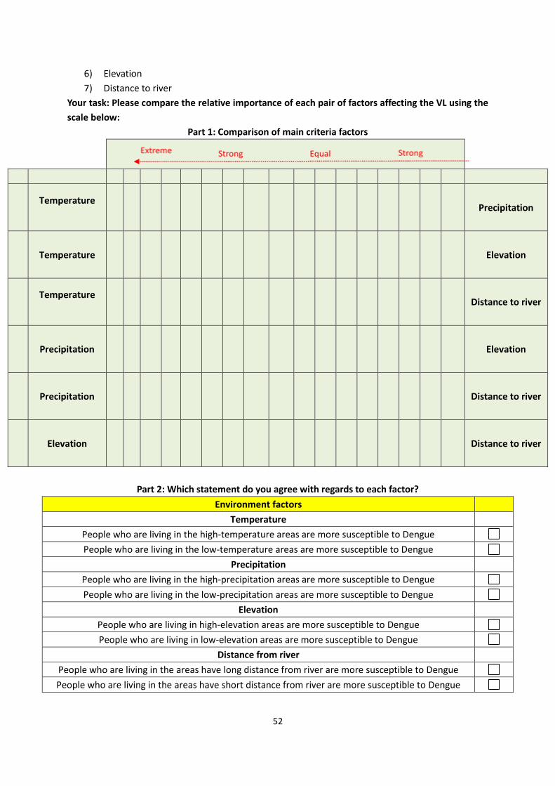
52
6) Elevation
7) Distance to river
Your task: Please compare the relative importance of each pair of factors affecting the VL using the
scale below:
Part 1: Comparison of main criteria factors
9 8 7 6 5 4 3 2 1 2 3 4 5 6 7 8 9
1 Temperature
Precipitation
2 Temperature Elevation
3 Temperature
Distance to river
4 Precipitation Elevation
5 Precipitation Distance to river
6 Elevation Distance to river
Part 2: Which statement do you agree with regards to each factor?
Environment factors
Temperature
People who are living in the high-temperature areas are more susceptible to Dengue
People who are living in the low-temperature areas are more susceptible to Dengue
Precipitation
People who are living in the high-precipitation areas are more susceptible to Dengue
People who are living in the low-precipitation areas are more susceptible to Dengue
Elevation
People who are living in high-elevation areas are more susceptible to Dengue
People who are living in low-elevation areas are more susceptible to Dengue
Distance from river
People who are living in the areas have long distance from river are more susceptible to Dengue
People who are living in the areas have short distance from river are more susceptible to Dengue
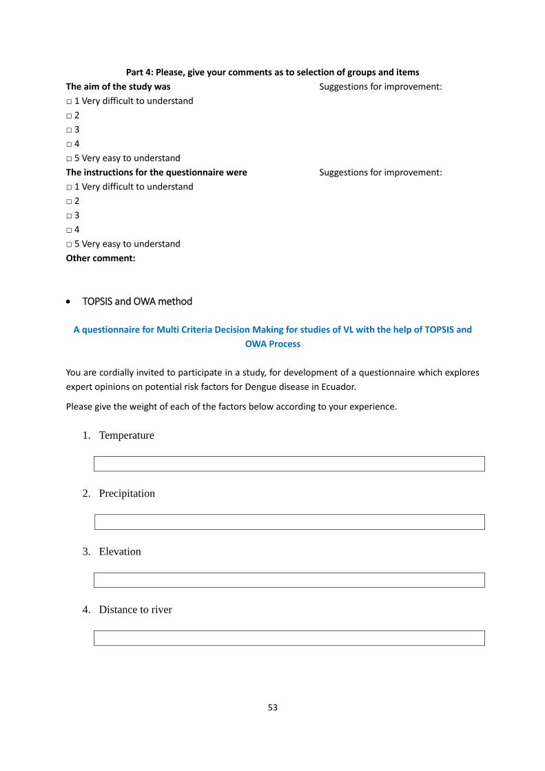
53
Part 4: Please, give your comments as to selection of groups and items
The aim of the study was Suggestions for improvement:
□ 1 Very difficult to understand
□ 2
□ 3
□ 4
□ 5 Very easy to understand
The instructions for the questionnaire were Suggestions for improvement:
□ 1 Very difficult to understand
□ 2
□ 3
□ 4
□ 5 Very easy to understand
Other comment:
TOPSIS and OWA method
A questionnaire for Multi Criteria Decision Making for studies of VL with the help of TOPSIS and
OWA Process
You are cordially invited to participate in a study, for development of a questionnaire which explores
expert opinions on potential risk factors for Dengue disease in Ecuador.
Please give the weight of each of the factors below according to your experience.
1. Temperature
2. Precipitation
3. Elevation
4. Distance to river
Top Related