


Languages
Pages
Legal


Postprint: Johannes Kamp & Matthias Kraume: Coalescence efficiency model including electrostatic interactions in liquid/liquid dispersions, Chem. Eng. Sci. 126 (2015) 132–142, http://dx.doi.org/10.1016/j.ces.2014.11.045
1
Coalescence efficiency model including electrostatic interactions
in liquid/liquid dispersions
Johannes Kamp1*, Matthias Kraume1
1Chair of Chemical & Process Engineering, Technische Universität Berlin,
Straße des 17. Juni 135, FH 6-1, 10623 Berlin, Germany
*Corresponding author: [email protected] Tel.: +49 30 314 23171
Abstract
The drop size distribution is an essential process variable in liquid/liquid systems and relevant in
many technical applications. It can be described by population balance equations. A coalescence
efficiency model was developed to be able to describe the well-known coalescence inhibition due to
changing pH value or salt concentration. The model includes the attractive van der Waals and re-
pulsive electrostatic force according to the DLVO theory into the population balance equation
framework. This DLVO model can extend existing simulations in a straightforward manner due to a
conceptual implementation. Moreover, zeta potential measurements were performed and the mod-
el was applied to simulate experiments in a stirred tank. Hence, the drop size distribution could be
predicted well with changing pH value. The results are discussed in comparison to simulations with
existing models in literature.
Keywords
population balance; coalescence; DLVO; electrostatic force; zeta potential; coalescence efficiency
1. Introduction
Liquid/liquid systems are an integral part of many unit operations in which the liquid phases are
either dispersed or separated. The drop size distribution which is the result of the competing phe-
nomena of drop breakage and coalescence determines a decisive part of the overall process effi-
ciency. Although these processes were investigated quite frequently, they are by no means com-
pletely understood.
The population balance equation (PBE) is a modelling approach which accounts for the droplet
interactions and describes the time dependent drop size distribution by death and birth terms for
drop breakage and coalescence (Hulburt and Katz, 1964; Kopriwa et al., 2012; Ramkrishna, 2000,
1985; Randolph and Larson, 1962). These terms consist of mechanistic sub models based on single
drop interactions depending on the drop size and system conditions (e.g. energy dissipation, viscos-
ities and interfacial tension). The modular concept of the population balance equation allows a
simple implementation and exchange of sub models which are available in literature for (I) drop
breakage (consisting of breakage rate and daughter drop size distribution) (Liao and Lucas, 2009)
and for (II) drop coalescence (consisting of collision frequency and coalescence efficiency) (Liao
and Lucas, 2010). The collision frequency determines the rate how often droplets in a system col-
lide with each other whereas the coalescence efficiency describes the probability that two interact-
ing drops merge into one. Together they form the coalescence rate. Up to now, a reliable prediction
of the coalescence rate and thus the drop size distribution accounting for all influencing chemical,
geometrical and process parameters is not available. Accordingly, further investigations and devel-
opments are necessary (Liao and Lucas, 2009). Existing models include influencing factors of the
chemical composition like density, viscosity and interfacial tension. But also other properties such
as the electrostatic interactions, which are not implemented properly so far, influence the coales-
cence significantly.

Postprint: Johannes Kamp & Matthias Kraume: Coalescence efficiency model including electrostatic interactions in liquid/liquid dispersions, Chem. Eng. Sci. 126 (2015) 132–142, http://dx.doi.org/10.1016/j.ces.2014.11.045
2
The coalescence of drops can be hindered by steric obstruction but also massively by electrochemi-
cal effects (Rambhau et al., 1977; Watanabe, 1984) up to a formation of a stable emulsion. A charge
separation induces an electrostatic potential at the interface of the droplets which again is damp-
ened by the solute ions in the continuous phase (Lyklema, 2000). Altogether, an electrostatic repul-
sive force results between two approaching droplets. However, this effect is not as easy to be im-
plemented in liquid/liquid systems as in the case of solid particles in an electrolyte solution. In the
latter case, the charged particle surface is surrounded by the electrical double layer: one fixed layer
of ions with opposing charge bound to the particle surface and a diffusive layer of ions dampening
the excess charge of the covered surface (Delgado et al., 2007; Israelachvili, 1991). Although the
reality is often more complex than this simple picture, the situation at a liquid/liquid interface is
even more complicated. A fixed layer of ions at a mobile interface seems to be quite unlikely. Con-
sequently, mobile ions at the surface will lead to a locally inhomogeneous charge due to movement
of the surface (Carroll, 1976). Additionally, it is known that the solubility of ions in oil is small
though non-zero (Izutsu, 2002; Wagner et al., 1998), inevitably a partition of the ions between the
two phases occurs and two electric ‘double’ layers are formed at both sides of the interphase
(Derjaguin et al., 1987). Although the induced potentials were measured by several authors, the
origin of the electrostatic potential at the interface is discussed in a controversial manner in litera-
ture. Some authors argue solely by means of dissimilar partition coefficients of the present ions in
the oil and water phase (Overbeek, 1952; Pfennig and Schwerin, 1998). Assuming different parti-
tion coefficients of the ions and applying the Albertsson model (Pfennig and Schwerin, 1998), it was
shown that only the relative magnitude of the partition coefficients may determine the potential
difference at the surface. Another widely used assumption is the preferred accumulation or adsorp-
tion of specific ions at the interface (especially hydroxide ions (Beattie and Djerdjev, 2004; Beattie
and Gray-Weale, 2012; Beattie et al., 2005; Creux et al., 2009; Franks et al., 2005; Gray-Weale and
Beattie, 2009; Marinova et al., 1996)), whether it is described by Gibbs (Lyklema, 2000) or Lang-
muir monolayers (Marinova et al., 1996; Tian and Shen, 2009). Other research groups doubt this
concept of ion adsorption and attribute the created potential to the immobilization and orientation
of water dipoles at the surface (Chibowski et al., 2005; Vacha et al., 2011) or to the deprotonation of
fatty acid impurities in the oil (Roger and Cabane, 2012a, 2012b).
The van der Waals force is the opposing attractive force acting on particles in the same range of
magnitude and distance (few tens of nanometres). The counter play of the repulsing electrostatic
and the attractive van der Waal force is well known as DLVO theory (Derjaguin and Landau, 1941;
Verwey and Overbeek, 1948). However, this theory has not been considered in population balance
equations up to now. The only model regarding electrostatic forces was published by Tobin and
Ramkrishna (1999), in which the authors introduce an additional varying parameter for the de-
scription of the repulse forces. An application and discussion of this model can be found in Kamp et
al. (2012) and a short summary in section 3.2.1.
Although there is no technically relevant model available describing the above mentioned ion phe-
nomena, there are several reports describing the influence of salts on liquid/liquid dispersions. The
investigations of Tobin and Ramkrishna (1992) in stirred liquid/liquid systems showed that an
increase in pH results in a decrease of drop sizes which was attributed to the coalescence inhibition
caused by adsorption of hydroxide ions at the interface and a resulting repulsive force. With addi-
tion of sodium chloride and therefore rising ionic strength, the coalescence inhibition was reduced
and the drop sizes in the system increased, which agrees with the DLVO theory. The decrease of the
drop size distribution at high pH values in a stirred tank is also described by Gäbler et al. (2006)
and Kraume et al. (2004). The authors explain this effect by an increasing coalescence inhibition
with higher pH values. Kraume et al. (2004) also showed the dependency of the coalescence inhibi-

Postprint: Johannes Kamp & Matthias Kraume: Coalescence efficiency model including electrostatic interactions in liquid/liquid dispersions, Chem. Eng. Sci. 126 (2015) 132–142, http://dx.doi.org/10.1016/j.ces.2014.11.045
3
tion from the NaCl concentration in shaken flask experiments. The settling time, meaning the time
after which a dispersed system is settled into two separate phases, increases with higher pH value
and decreases with higher salt concentration. Pfennig and Schwerin (1998) also found a strong
coalescence inhibition in batch settling experiments adding NaCl and NaBr to a water in 1-butanol
emulsion. According to the DLVO theory, they found the depletion of the coalescence inhibition
with further increased salt concentration due to the dampening behaviour of the ions in the diffu-
sive electrical layer.
The influence of salts on droplet coalescence was investigated by Villwock et al. (2014) observing
the collision of two single droplets. A decrease of coalescence probability was found with the addi-
tion of both NaOH and NaCl. Accordingly, Dunstan (1992) observed chloride adsorption on hydro-
carbon particles and found an increasing zeta potential with higher KCl concentration. He explained
this by a preferential solubility of Cl- ions near the surface and not by adsorption. Marinova et. al
(1996) found OH- being the potential determining ion in xylene/water emulsions by performing
zeta potential measurements with varying pH at an ionic strength of I = 10-3 mol/L. Tian and Shen
(2009) investigated the adsorption of H3O+, OH- and Cl- at the octadecyltrichlorosilane/water inter-
face and found the adsorption of OH- to be preferential against Cl- and H3O+. Considering these men-
tioned publications it becomes obvious that Cl- has to be considered besides OH- if studying the
surface potential in a system containing those ions.
Another interesting fact is the small influence of the oil phase in this context. Marinova et. al (1996)
investigated emulsions of different non-polar oils (xylene, dodecane, hexadecane and perfluorome-
thyldecalin) and found practically the same zeta potential under identical experimental conditions
for all systems. This result was confirmed by the investigations of Creux et al. (2009) who found
similar pH dependencies of the zeta potential of nitrobenzene, benzene, octane, decane and dodec-
ane. Thus, the electrostatic effects appear to be nearly independent from the type of oil, and zeta
potential measurements of one specific oil can be adopted universally.
2. Materials & methods
All experiments were carried out using water as continuous and toluene as disperse phase. To set
the pH value and the ionic strength sodium hydroxide, hydrochloric acid and sodium chloride were
used. All equipment used was made of glass, stainless steel or PTFE where possible. Serious effort
was made in all set-ups to avoid contaminations. Hence all equipment was cleaned thoroughly and
rinsed with deionised water extensively prior to use.
2.1. Experimental investigations in stirred tank
The experiments were performed by Wegener (2004) previously at our institute and were pub-
lished partly in the PhD thesis of Gäbler (2007) and in Kamp et al. (2012). To detect the drop size
distribution (at T = 293 K) in a baffled stirred tank DN150 (H/D = 1) equipped with a Rushton tur-
bine (d/D = 0.33) an endoscope technique was used. For detailed description of this set-up and
measurement technique see Maaß et al. (2011) and Ritter and Kraume (2000). Continuous phase
was deionised water with added NaOH (Merck 1.09956 p.a.), NaCl (Merck 1.06404 p.a.) and HCl
(Merck 1.09970 p.a.) to set pH and a constant ionic strength (I = 0.1 mol/L). As disperse phase tolu-
ene was used with a volumetric phase fraction of φ = 0.1. The drop size distributions were meas-
ured for the pH values 1, 3, 5, 7, 9, 11 and 13 each with three stirrer frequencies (n = 400, 550,
700 min-1) at distinct times after the start of the impeller. The experimental stirrer frequencies
correspond to mean energy dissipation rates in the stirred tank of ϵ = 0.133, 0.345 and 0.712 m2/s3.
Postprint: Johannes Kamp & Matthias Kraume: Coalescence efficiency model including electrostatic interactions in liquid/liquid dispersions, Chem. Eng. Sci. 126 (2015) 132–142, http://dx.doi.org/10.1016/j.ces.2014.11.045
4
2.2. Experimental determination of electrophoretic mobility
The sample preparation was done in a similar manner to the procedure applied by Marinova et al.
(1996). The pH of the water continuous phase (ultrapure water with a resistivity of 18.3 MΩ·cm,
produced by the purification system Merck Millipore Milli-Q Gradient) was adjusted with hydro-
chloric acid (Merck 1.09970 p.a.) and accordingly sodium hydroxide (Merck 1.09956 p.a.). To set a
constant ionic strength of I = 0.1 mol/L, sodium chloride (Merck 1.06404 p.a.) was added respec-
tively. Due to the sensitive unbuffered aqueous solution, the pH was measured by a pH-meter
(WTW pH197) and indicator strips (VWR ProLabo Dosatest 3 zones). Due to the minor effect of
dissolved carbon dioxide (CO2 / HCO3- / CO3
2-) reported by Marinova et al. (1996), a purging of CO2
with N2 was omitted. Nevertheless, all serial dilutions and samples were closed as fast as possible to
minimize the contact with the atmosphere and an additional dissolution of CO2. The samples were
each prepared with 10 mL water continuous phase and 3 - 5 mL toluene (Fluka 89681-2.5L p.a.) in
20 mL vials with a magnetic stirrer. These vials were stirred and heated to 65°C in a water bath for
at least 2 hours to increase the solubility of toluene in the water phase (Jou and Mather, 2003;
Tsonopoulos, 2001). Prior to a measurement, the respective sample was cooled down rapidly to
25°C by rinsing with tap water from the outside, which causes a precipitation of the excess toluene
in the water phase. The generated emulsion with a drop size distribution between dp ≈ 2 - 7 m and
a mean diameter of dm = 5 m (measured with Malvern Zetasizer Nano ZS) remained stable for
analysis for about 15 minutes.
Electrophoretic mobility ue was measured at 25 ± 0.1 °C using a Malvern Zetasizer Nano ZS with
disposable cuvettes Malvern DTS1060. These were used because the application of the solvent re-
sistant dip cell provided by Malvern resulted in a degradation of the toluene and / or the palladium
electrodes to dark brown residua during measurements. Even though the disposable cuvettes were
blurred by the toluene after several runs, equivalent results could be gained reusing these cuvettes
and the results of Marinova et al. (1996) could be reproduced. Additionally, the phase fraction of
toluene of the investigated emulsion was below 0.1%, which minimises the chance of a dissociation
of contaminants from the disposable cuvettes by toluene during the short time of measurement
(approximately 30 seconds). For every pH value at least two separate samples were prepared and
measured in several runs each, resulting in approx. 30 - 60 single measurement runs per pH value.
The ‘general purpose’ mode of Malvern Zetasizer Nano ZS was used, thus every value from a single
measurement run represents the mean value of the zeta potential distribution.
2.3. Numerical investigations & parameter estimation
In this study the experimental drop size distributions in a stirred tank were simulated using an
integral single zone PBE of the whole tank with a mean energy input ϵ generated by the impeller.
The volume-related PBE for this batch reactor describing the time dependent number density func-
tion 𝑓(𝑑𝑝 , 𝑡) of drops with diameter dp becomes (Attarakih et al., 2004; Gäbler et al., 2006; Liao and
Lucas, 2009):
𝜕𝑓(𝑑𝑝, 𝑡)
𝜕𝑡= ∫ 𝑛𝑑(𝑑𝑝
′ ) ∙ 𝛽(𝑑𝑝, 𝑑𝑝′ ) ∙ 𝑔(𝑑𝑝
′ ) ∙ 𝑓(𝑑𝑝′ , 𝑡) d𝑑𝑝
′ − 𝑔(𝑑𝑝) ∙ 𝑓(𝑑𝑝 , 𝑡)
𝑑𝑝,𝑚𝑎𝑥
𝑑𝑝
+1
2∫ 𝜉(𝑑𝑝
′′ , 𝑑𝑝′ ) ∙ 𝜆(𝑑𝑝
′′ , 𝑑𝑝′ ) ∙ 𝑓(𝑑𝑝
′ , 𝑡) ∙ 𝑓(𝑑𝑝′′ , 𝑡) d𝑑𝑝
′
𝑑𝑝
0
− 𝑓(𝑑𝑝, 𝑡) ∙ ∫ 𝜉(𝑑𝑝 , 𝑑𝑝′ ) ∙ 𝜆(𝑑𝑝, 𝑑𝑝
′ ) ∙
𝑑𝑝,𝑚𝑎𝑥−𝑑𝑝
0
𝑓(𝑑𝑝′ , 𝑡) d𝑑𝑝
′
1
Postprint: Johannes Kamp & Matthias Kraume: Coalescence efficiency model including electrostatic interactions in liquid/liquid dispersions, Chem. Eng. Sci. 126 (2015) 132–142, http://dx.doi.org/10.1016/j.ces.2014.11.045
5
consisting of the number of daughter droplets nd, daughter drop size distribution 𝛽(𝑑𝑝, 𝑑𝑝′ ), break-
age rate 𝑔(𝑑𝑝), collision frequency 𝜉(𝑑𝑝, 𝑑𝑝′ ) and coalescence efficiency 𝜆(𝑑𝑝, 𝑑𝑝
′ ) and using the
definition 𝑑𝑝′′ = (𝑑𝑝
3 − 𝑑𝑝′ 3)
13⁄. The detailed description of the PBE, the sub model implementation
and numerical parameter definition is reported in Kamp et al. (2012). As this article focusses on the
coalescence efficiency, the other sub models of collision frequency and drop breakage which are
necessary to solve the PBE were taken from the frequently used model of Coulaloglou and
Tavlarides (1977). The coalescence efficiency sub models of Coulaloglou and Tavlarides (1977) and
Tobin and Ramkrishna (1999) were compared with regard to the description of the coalescence
inhibition due to electrostatic effects. Furthermore, a new coalescence efficiency sub model was
developed in order to describe this inhibition properly. Concerning the droplet breakup, an effec-
tive daughter drop size distribution should have no singularities and fall to zero as the ratio be-
tween mother and daughter drop diameter becomes zero or one (Maaß et al., 2007; Wang et al.,
2003; Zaccone et al., 2007). Otherwise, a droplet breakup would cause a loss of mass and violate the
mass balance. Since the daughter drop size distribution of the Coulaloglou and Tavlarides (1977)
model is implemented as a normal distribution, it does not fulfil the mentioned requirements. Thus,
a relatively narrow normal distribution was applied for the binary droplet breakup (number of
daughter droplets nd = 2) of a droplet with volume 𝑉𝑝: a mean daughter drop volume 𝑉𝜇 =𝑉𝑝
𝑛𝑑 and a
standard deviation of 𝑉𝜎 =𝑉𝑝
5𝑛𝑑 was used. Using these parameters >99.9% of droplets formed lay
within the volume range from 0 to Vp and the mass balance could be conserved adequately.
The commercial software PARSIVAL® (Wulkow et al., 2001) was used to solve the partial differential
equation of the PBE with coupled mass balance.
The numerical parameters of the breakage and coalescence rate of the different models were fitted
to experimental data using the implemented parameter estimation routine by minimising the re-
sidual between experimental and simulated data. To quantify this residual between n experimental
values 𝑋𝑖 and calculated ones �̂�𝑖 , the root-mean-square deviation (RMSD) was used in this work:
RMSD(𝑋) = √∑ (𝑋𝑖−�̂�𝑖)2𝑛
𝑖=1
𝑛 . 2
At the beginning, all parameters of the basic Coulaloglou and Tavlarides (1977) model were opti-
mized to the transient development of the Sauter mean diameter d32 at pH 7. To provide compara-
bility between the models, these fitted parameters for drop breakage (c1,b and c2,b) and collision
frequency (c1,c) were kept constant throughout the whole study. For the coalescence efficiency sub
model(s) the corresponding ‘hydrodynamic’ parameter c2,c was also adapted to pH 7 and the ‘elec-
trostatic’ parameter c3,c was adjusted to transient data of d32 at pH 13. All parameters are given in SI
units if dimensional: c2,c of the Coulaloglou and Tavlarides (1977) model has the dimension [m-2]
and c3,c of the Tobin and Ramkrishna (1999) model is not dimension consistent and would have the
dimension [N/m] and/or [N/m2]. For detailed information of the model implementation and nu-
merical parameter definition see Kamp et al. (2012).
All simulations were verified to be independent from the initial drop size distribution after a few
seconds or iteration steps, respectively. Thus, a Gaussian initial drop size distribution with a mean
value 𝑑𝜇 = 1 mm and standard deviation 𝑑𝜎 = 50 μm was used arbitrarily.
The interfacial tension was set to = 35 mN/m for all simulations with pH < 12.5. For pH > 12.5
= 32 mN/m was used according to the measurements performed by Kamp et al. (2012). Anyhow,
the influence of the change in interfacial tension is rather small in the simulations: the reduction
from = 35 mN/m to 32 mN/m leads to a decrease of the steady state Sauter mean diameter of
approximately 𝑑32,𝑠𝑡𝑎𝑡 ≈ 15 μm.

Postprint: Johannes Kamp & Matthias Kraume: Coalescence efficiency model including electrostatic interactions in liquid/liquid dispersions, Chem. Eng. Sci. 126 (2015) 132–142, http://dx.doi.org/10.1016/j.ces.2014.11.045
6
3. Results & discussion
As already pointed out in the introduction, the origin of the surface potential in liquid/liquid sys-
tems is discussed controversially in literature until present. However, a description and quantifica-
tion of the surface potential is inevitable to implement the DLVO theory into the population balance
equation. Hence, the following approach was chosen: the ions were assumed to accumulate at (or
near) the interface and the anions OH- and Cl- were identified to be potential determining. The ac-
cumulation of these ions was described by a Stern isotherm for which the surface potential was
investigated by zeta potential measurements. This approach is presented and discussed in the fol-
lowing and then used to develop the coalescence model which is compared with existing models in
literature.
3.1. Zeta potential investigations
The electrophoretic mobility ue was measured varying the pH value from pH = 2 to 13 at constant
ionic strength of I = 0.1 mol/L according to the procedure described in section 2.2. With the meas-
ured drop radius of a = 2.5 m, the resulting ·a = 259 fulfils the restriction of the Helmholtz-
Smoluchowski equation (·a >> 1) (Delgado et al., 2007; Smoluchowski, 1903). Thus, zeta potential
was calculated from electrophoretic mobility originally measured by the Zetasizer Nano ZS, alt-
hough the Helmholtz-Smoluchowski equation is applicable only for rigid particles. Nevertheless, it
is used because the presence of the double layer is assumed to result in a reduced momentum
transfer to the drop phase according to Delgado et al. (2007). Likewise, Lyklema (2000) regards the
neglect of a mobile interface as more appropriate for liquid/liquid than for gas/liquid interfaces
which is obvious having a viscosity change in the order of several magnitudes from gas to oil. The
measured electrophoretic mobility and the calculated zeta potential over the pH range are shown in
Figure 1. The vertical error bars represent the standard deviation between all measured values. The
highest deviation in the measured zeta potential was measured in the sample with pH between 9
and 10. However, this data point seems to be an outlier in Figure 1. The horizontal error bars indi-
cate the standard deviation of the pH values measured in the serial dilutions and samples at differ-
ent times. Especially the samples prepared with ion concentrations resulting in pH values from 6 to
10 show a shift to lower pH value due to absorption of carbon dioxide from the atmosphere and
therefore result in pH deviations. However, the presence of carbon dioxide in the continuous water
phase due to absorption did not have an observable effect on the zeta potential which was also
reported by Marinova et al. (1996). At very acidic conditions the pH deviation becomes so small
that the error bars are covered by the symbols.

Postprint: Johannes Kamp & Matthias Kraume: Coalescence efficiency model including electrostatic interactions in liquid/liquid dispersions, Chem. Eng. Sci. 126 (2015) 132–142, http://dx.doi.org/10.1016/j.ces.2014.11.045
7
Figure 1: Zeta potential and electrophoretic mobility over pH value, the specific surface coverage of Cl- and OH- (Equation 5) from the adsorption isotherm (Equation 3) and the corresponding surface potential Ψs (Equation 6) and its numerical fit (Equation 15) at constant ionic strength I = 0.1 mol/L in toluene/water system.
The zeta potential was found to scatter around a constant value of about -15 mV for pH < 9, which
can be explained by the adsorption of Cl- at (or near) the interface. For higher pH values a strong
decrease of the zeta potential down to -42 mV was found which corresponds to the replacement of
Cl- with OH- ions due to the higher bulk concentration of hydroxide. The specific coverages of the
surface θCl- and θOH- and the resulting surface potential Ψs were calculated with an adsorption iso-
therm and the Grahame equation as described in the following and are shown in Figure 1.
According to Marinova et al. (1996) and Derjaguin et al. (1987), the ion accumulation is described
by a Stern adsorption isotherm (Derjaguin, 1989; Stern, 1924):
Γi =Γ0𝜐𝑖𝑛𝑖,0exp (−
Φ𝑖 + 𝑧𝑖𝑒Ψs
𝑘𝐵𝑇)
1 + ∑ 𝜐𝑖𝑛𝑖,0exp (−Φ𝑖 + 𝑧𝑖𝑒Ψs
𝑘𝐵𝑇)𝑖
3
where i is the number of type i ions per surface area which is described by the ion specific parame-
ters: i the volume of a hydrated ion, ni,0 the number concentration in bulk, zi the valence; the physi-
cal constants: e the elementary charge and kB the Boltzmann constant; the system specific parame-
ters: surface potential s, temperature T and the fitted parameters: 0 the referenced saturation
adsorption, i the specific interaction energy of ion i. The Stern isotherm becomes a Langmuir iso-
therm for zi = 0. In this study not only the adsorption of OH- was considered as done by Marinova et
al. (1996) but additionally the adsorption of Cl- to describe the low potentials of about -15 mV for
pH < 9. The relation between the surface charge density and the surface potential s is given by
the Grahame equation (Butt et al., 2003; Israelachvili, 1991):
𝜎 = √8𝜀𝑟𝜀0𝑘𝐵𝑇𝑛𝑠𝑎𝑙𝑡,0sinh (𝑒Ψ𝑠
2𝑘𝐵𝑇) 4
where r is the relative and 0 the vacuum permittivity and nsalt,0 the number concentration of the
salts in the bulk. In the case of monovalent ions nsalt,0 is equivalent to the number concentration of
0.0
0.1
0.2
0.3
0.4
0.5
0.6
0.7
0.8
0.9
1.0
0 1 2 3 4 5 6 7 8 9 10 11 12 13 14
spec
ific
su
rfac
e co
vera
ge θ
[-]
zeta
po
ten
tial
ζ[m
V]
pH
Mittelwerte Dez. 2011
Isotherme
Isotherme fit
theta_Cl
theta_OH
-51.00
-41.00
-31.00
-21.00
-11.00
-1.00
-4
-3
-2
-1
0
0 1 2 3 4 5 6 7 8 9 10 11 12 13 14
ele
ctr
op
ho
rectic m
ob
ility
[1
0-8
m²/
Vs]
pH
Mittelwerte Dez. 2011
Mittelwerte Aug. 2011
Isotherme
Isotherme fit
0
-10
-20
-30
-40
-50
-1
-2
-3
Ele
ctro
ph
ore
tic
mo
bil
ity
ue
[10
-8 m
²/(V
∙s)]
Spec
ific
su
rfac
e co
ver
age
θi [
-]
Surf
ace
po
ten
tial
Ψs,
zeta
po
ten
tial
ζ [
mV
]
0.0
0.1
0.2
0.3
0.4
0.5
0.6
0.7
0.8
0.9
1.0
0 1 2 3 4 5 6 7 8 9 10 11 12 13 14
sp
ecific
surf
ace
co
vera
ge
θ[-
]
zeta
po
tentia
l ζ
[mV
]
pH
Mittelwerte Dez. 2011
Mittelwerte Aug. 2011
Isotherme
Isotherme fit
theta_Cl
theta_OH
Measurements ue / ζ
Surface potential Ψs (Eq. 6)
Numerical fit Ψs (Eq. 15)
Surface coverage θCl-
Surface coverage θOH-
0.0
0.1
0.2
0.3
0.4
0.5
0.6
0.7
0.8
0.9
1.0
0 1 2 3 4 5 6 7 8 9 10 11 12 13 14
sp
ecific
surf
ace
co
vera
ge
θ[-
]
zeta
po
tentia
l ζ
[mV
]
pH
Mittelwerte Dez. 2011
Mittelwerte Aug. 2011
Isotherme
Isotherme fit
theta_Cl
theta_OH
0.0
0.1
0.2
0.3
0.4
0.5
0.6
0.7
0.8
0.9
1.0
0 1 2 3 4 5 6 7 8 9 10 11 12 13 14
sp
ecific
surf
ace
co
vera
ge
θ[-
]
zeta
po
tentia
l ζ
[mV
]
pH
Mittelwerte Dez. 2011
Mittelwerte Aug. 2011
Isotherme
Isotherme fit
theta_Cl
theta_OH
0.0
0.1
0.2
0.3
0.4
0.5
0.6
0.7
0.8
0.9
1.0
0 1 2 3 4 5 6 7 8 9 10 11 12 13 14
sp
ecific
surf
ace
co
vera
ge
θ[-
]
zeta
po
tentia
l ζ
[mV
]
pH
Mittelwerte Dez. 2011
Mittelwerte Aug. 2011
Isotherme
Isotherme fit
theta_Cl
theta_OH
0.0
0.1
0.2
0.3
0.4
0.5
0.6
0.7
0.8
0.9
1.0
0 1 2 3 4 5 6 7 8 9 10 11 12 13 14
sp
ecific
surf
ace
co
vera
ge
θ[-
]
zeta
po
tentia
l ζ
[mV
]
pH
Mittelwerte Dez. 2011
Mittelwerte Aug. 2011
Isotherme
Isotherme fit
theta_Cl
theta_OH

Postprint: Johannes Kamp & Matthias Kraume: Coalescence efficiency model including electrostatic interactions in liquid/liquid dispersions, Chem. Eng. Sci. 126 (2015) 132–142, http://dx.doi.org/10.1016/j.ces.2014.11.045
8
the dissolved anions (or cations) or the ionic strength times the Avogadro constant: 𝐼 ∙ 𝑁𝐴. It is as-
sumed here that the surface potential s is determined by the anions OH- and Cl- and that it is equal
to the zeta potential. The surface coverage of an adsorbed ion i is derived from the Stern adsorption
isotherm (Equation 3):
θ𝑖 =Γ𝑖
Γ0 . 5
Additionally, the total charge induced by the ion coverage (∑ 𝑧𝑖𝑒𝜃𝑖𝑖 ) has to equal the surface charge
density given by the Grahame equation (Equation 4) (Marinova et al., 1996):
−𝑒(θOH− + θ𝐶𝑙−) = 𝜎 . 6
To obtain the graph shown in Figure 1, both sides of the Equation 6 were solved iteratively using
the least-squares method to identify the surface potential s with varying pH and thus specific ion
concentrations. To fit the zeta potential measurements the values of the saturation adsorption
0 = 2.3185·1017 m-² and the specific interaction energies OH- = -9.50 kB·T and Cl- = -4.25 kB·T
were determined manually in the Stern isotherm. The volumes of the hydrated ions were imple-
mented as OH- = 1.1·10-28 m³ (Israelachvili, 1991) and Cl- = 1.5·10-28 m³ (David et al., 2001;
Israelachvili, 1991). According to the results of Tian and Shen (2009), the adsorption of OH- was
found to be preferential against Cl-. Additionally, the surface coverage of Cl- is located in the same
range (Cl- = 0.20) as in our case (Cl- = 0.27). Moreover, the measured increase of the zeta potential
for pH < 3 (see Figure 1) could be explained by the additional adsorption of H3O+ under these condi-
tions which was found by Tian and Shen (2009). As this influence is rather small and not significant
in this case, it is not modelled here.
Despite the previously discussed limitations of this measurement technique, the zeta potential is a
feasible technique to gain at least qualitative influences on the surface potential and thus on the
emulsion stability (Lyklema, 2000; Marinova et al., 1996; Rambhau, 1978), although the measured
value may not be equal with the existent surface potential (however it is induced) (Delgado et al.,
2007).
The use of a Gibbs isotherm may be more appropriate in the case of liquid/liquid systems (Lyklema,
2000), but significant surface tension measurements were not available. A decrease in the surface
tension from = 35 to 32 mN/m was found as reported in Kamp et al. (2012), but the standard de-
viation increased considerably at high pH. Additionally, Derjaguin et al. (1987) discussed the con-
sideration of Gibbs free energy and a formation of a double layer at both sides of the interface (in oil
and water phase respectively) and thus obtained the same functional relation for the electrostatic
force as in the case of Stern adsorption. However, the Stern isotherm is used to describe the trend
of the zeta potential over pH value which is again simplified by a numerical fit in the developed
model due to a reduction of computation time (see chapter 3.2.2). Thus, the described approach is
regarded as adequate.
3.2. Modelling & simulation
This section begins with an application of the coalescence efficiency sub models of Coulaloglou and
Tavlarides (1977) and Tobin and Ramkrishna (1999) to the coalescence inhibition found at high pH
values. Afterwards, the new modelling approach is developed and discussed.
3.2.1. Simulations with existing models
As discussed in detail in Kamp et al. (2012), the model of Coulaloglou and Tavlarides (1977) is able
to describe the experimental data by varying only the numerical parameter c2,c of the coalescence
efficiency. These findings are presented shortly in the following with the difference to Kamp et al.
(2012) that no additional prefactor of the energy dissipation rate was used (fϵ = 1) as suggested in
Kamp et al. (2012). This prefactor was formerly considered to account for inhomogeneous energy
Postprint: Johannes Kamp & Matthias Kraume: Coalescence efficiency model including electrostatic interactions in liquid/liquid dispersions, Chem. Eng. Sci. 126 (2015) 132–142, http://dx.doi.org/10.1016/j.ces.2014.11.045
9
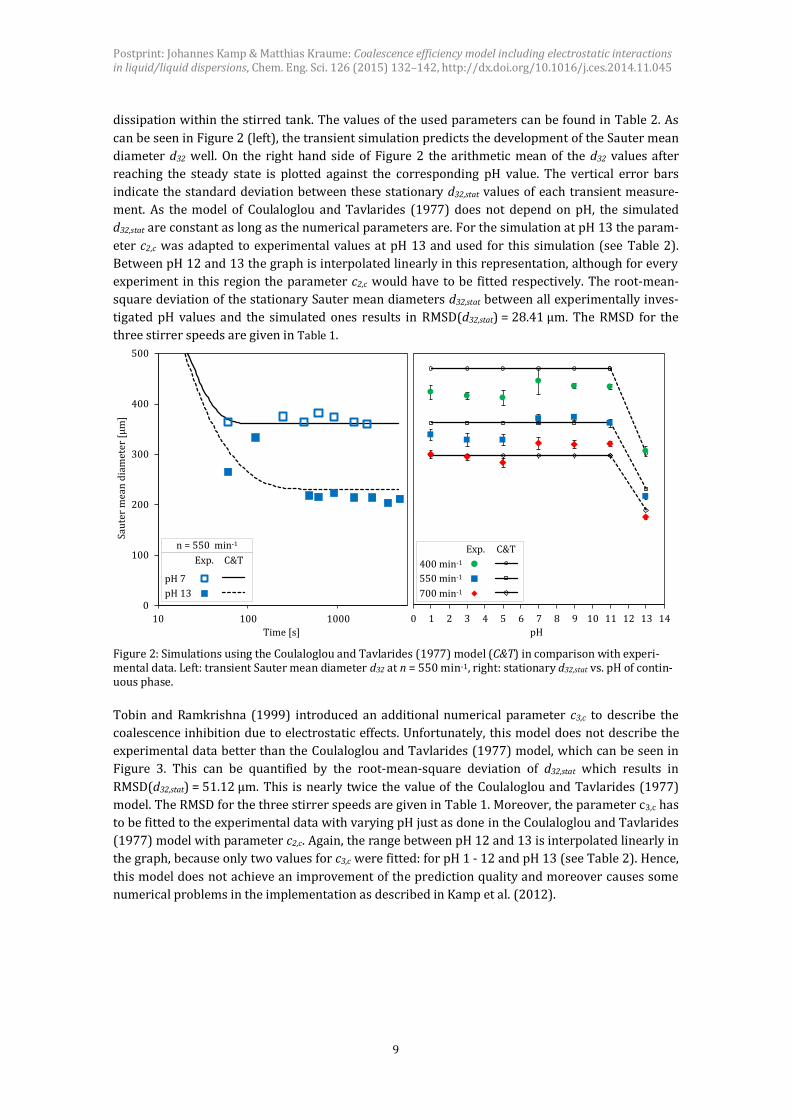
dissipation within the stirred tank. The values of the used parameters can be found in Table 2. As
can be seen in Figure 2 (left), the transient simulation predicts the development of the Sauter mean
diameter d32 well. On the right hand side of Figure 2 the arithmetic mean of the d32 values after
reaching the steady state is plotted against the corresponding pH value. The vertical error bars
indicate the standard deviation between these stationary d32,stat values of each transient measure-
ment. As the model of Coulaloglou and Tavlarides (1977) does not depend on pH, the simulated
d32,stat are constant as long as the numerical parameters are. For the simulation at pH 13 the param-
eter c2,c was adapted to experimental values at pH 13 and used for this simulation (see Table 2).
Between pH 12 and 13 the graph is interpolated linearly in this representation, although for every
experiment in this region the parameter c2,c would have to be fitted respectively. The root-mean-
square deviation of the stationary Sauter mean diameters d32,stat between all experimentally inves-
tigated pH values and the simulated ones results in RMSD(d32,stat) = 28.41 μm. The RMSD for the
three stirrer speeds are given in Table 1.
Figure 2: Simulations using the Coulaloglou and Tavlarides (1977) model (C&T) in comparison with experi-mental data. Left: transient Sauter mean diameter d32 at n = 550 min-1, right: stationary d32,stat vs. pH of contin-uous phase.
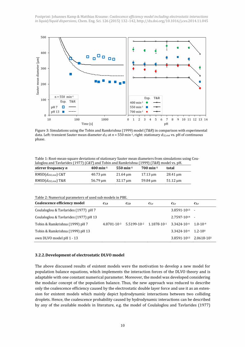
Tobin and Ramkrishna (1999) introduced an additional numerical parameter c3,c to describe the
coalescence inhibition due to electrostatic effects. Unfortunately, this model does not describe the
experimental data better than the Coulaloglou and Tavlarides (1977) model, which can be seen in
Figure 3. This can be quantified by the root-mean-square deviation of d32,stat which results in
RMSD(d32,stat) = 51.12 μm. This is nearly twice the value of the Coulaloglou and Tavlarides (1977)
model. The RMSD for the three stirrer speeds are given in Table 1. Moreover, the parameter c3,c has
to be fitted to the experimental data with varying pH just as done in the Coulaloglou and Tavlarides
(1977) model with parameter c2,c. Again, the range between pH 12 and 13 is interpolated linearly in
the graph, because only two values for c3,c were fitted: for pH 1 - 12 and pH 13 (see Table 2). Hence,
this model does not achieve an improvement of the prediction quality and moreover causes some
numerical problems in the implementation as described in Kamp et al. (2012).
0
100
200
300
400
500
10 100 1000
Time [s] pH
Sau
ter
mea
n d
iam
eter
[μ
m]
0 1 2 3 4 5 6 7 8 9 10 11 12 13 14
0
100
200
300
400
500
10 1000
550rpm pH 7
550rpm pH13
sim pH7
sim pH13
0
100
200
300
400
500
10 1000
550rpm pH 7
550rpm pH13
sim pH7
sim pH13
Exp. C&T
pH 7
pH 13
Exp. C&T
400 min-1
01234567891011121314
400 rpm
550 rpm
700 rpm
sim400 pH1-11
sim550 pH1-11
sim700 pH1-11
sim400 pH11-13
sim550 pH11-13
sim700 pH11-13
01234567891011121314
400 rpm
550 rpm
700 rpm
sim400 pH1-11
sim550 pH1-11
sim700 pH1-11
sim400 pH11-13
sim550 pH11-13
sim700 pH11-13
550 min-1
700 min-1
n = 550 min-1
Postprint: Johannes Kamp & Matthias Kraume: Coalescence efficiency model including electrostatic interactions in liquid/liquid dispersions, Chem. Eng. Sci. 126 (2015) 132–142, http://dx.doi.org/10.1016/j.ces.2014.11.045
10
Figure 3: Simulations using the Tobin and Ramkrishna (1999) model (T&R) in comparison with experimental data. Left: transient Sauter mean diameter d32 at n = 550 min-1, right: stationary d32,stat vs. pH of continuous phase.
Table 1: Root-mean-square deviations of stationary Sauter mean diameters from simulations using Cou-laloglou and Tavlarides (1977) (C&T) and Tobin and Ramkrishna (1999) (T&R) model vs. pH.
stirrer frequency n 400 min-1 550 min-1 700 min-1 total
RMSD(dd32,stat) C&T 40.73 μm 21.64 μm 17.13 μm 28.41 μm
RMSD(dd32,stat) T&R 56.79 μm 32.17 μm 59.84 μm 51.12 μm
Table 2: Numerical parameters of used sub models in PBE.
Coalescence efficiency model c1,b c2,b c1,c c2,c c3,c
Coulaloglou & Tavlarides (1977) pH 7 3.8591·1013 -
Coulaloglou & Tavlarides (1977) pH 13 2.7597·1014 -
Tobin & Ramkrishna (1999) pH 7 4.8701·10-3 5.5199·10-2 1.1878·10-1 3.3424·10-4 1.0·10-9
Tobin & Ramkrishna (1999) pH 13 3.3424·10-4 1.2·100
own DLVO model pH 1 - 13 3.8591·1013 2.0618·103
3.2.2. Development of electrostatic DLVO model
The above discussed results of existent models were the motivation to develop a new model for
population balance equations, which implements the interaction forces of the DLVO theory and is
adaptable with one constant numerical parameter. Moreover, the model was developed considering
the modular concept of the population balance. Thus, the new approach was reduced to describe
only the coalescence efficiency caused by the electrostatic double layer force and use it as an exten-
sion for existent models which mainly depict hydrodynamic interactions between two colliding
droplets. Hence, the coalescence probability caused by hydrodynamic interactions can be described
by any of the available models in literature, e.g. the model of Coulaloglou and Tavlarides (1977)
0 1 2 3 4 5 6 7 8 9 10 11 12 13 14
0
100
200
300
400
500
10 100 1000
Time [s] pH
Sau
ter
mea
n d
iam
eter
[μ
m]
0
100
200
300
400
500
10 1000
550rpm pH 7
550rpm pH13
sim pH7
sim pH13
0
100
200
300
400
500
10 1000
550rpm pH 7
550rpm pH13
sim pH7
sim pH13
Exp. T&R
pH 7
pH 13
Exp. T&R
400 min-1
01234567891011121314
400 rpm
550 rpm
700 rpm
sim400 pH1-11
sim550 pH1-11
sim700 pH1-11
sim400 pH11-13
sim550 pH11-13
sim700 pH11-13
01234567891011121314
400 rpm
550 rpm
700 rpm
sim400 pH1-11
sim550 pH1-11
sim700 pH1-11
sim400 pH11-13
sim550 pH11-13
sim700 pH11-13
550 min-1
700 min-1
n = 550 min-1

Postprint: Johannes Kamp & Matthias Kraume: Coalescence efficiency model including electrostatic interactions in liquid/liquid dispersions, Chem. Eng. Sci. 126 (2015) 132–142, http://dx.doi.org/10.1016/j.ces.2014.11.045
11
(which explicitly excludes the van der Waals and double layer forces). Regarding the two coales-
cence inhibition processes (hydrodynamic and electrostatic) as independent from one another, the
total coalescence efficiency becomes:
λ = 𝜆ℎ𝑦𝑑𝑟𝑜𝑑𝑦𝑛𝑎𝑚𝑖𝑐 ∙ 𝜆𝐷𝐿𝑉𝑂 . 7
Following this modelling approach, the electrostatic coalescence inhibition can be implemented
easily in simulations if necessary.
The implementation of the DLVO interactions follows the functional approach of Coulaloglou and
Tavlarides (1977). They assume that the coalescence occurs if the contact time exceeds the time
which is needed until the thin film of continuous phase between the drops is drained. Assuming the
contact time being a normally distributed random variable, these counteracting times determine
the coalescence probability by the functional approach:
λC&T ∝ exp (−𝑡𝑑𝑟𝑎𝑖𝑛𝑎𝑔𝑒
𝑡𝑐𝑜𝑛𝑡𝑎𝑐𝑡) . 8
In the case of DLVO interactions, the counteracting repulsive electrostatic double layer force Fel and
attractive van der Waals force FvdW depend on the distance h between two approaching droplets.
This distance and therefore the two forces vary with the contact time of two droplets and are as-
sumed to be normally distributed random variables. Hence, the same functional approach is used to
describe the electrostatic coalescence probability depending on the ratio between Fel and the abso-
lute value of FvdW:
λ𝐷𝐿𝑉𝑂 ∝ exp (−𝐹𝑒𝑙
|𝐹𝑣𝑑𝑊|) . 9
Considering the approach of Derjaguin (1934) to calculate these forces for curved surfaces, the
electrostatic double layer force for two approaching droplets is given for symmetrical electrolytes
by Derjaguin et al. (1987) and Miller and Neogi (2008):
𝐹𝑒𝑙 = 32𝜋𝜀0𝜀𝑟𝜅𝑅𝑒𝑞 (𝑘𝐵𝑇
𝑧𝑒)
2
tanh2 (zeΨ𝑠
4𝑘𝐵𝑇) exp(−𝜅ℎ) 10
assuming the surface potential being constant during approach, where Req is the equivalent drop
radius of the two approaching droplets with the diameters d1 and d2:
𝑅𝑒𝑞 =𝑑1∙𝑑2
𝑑1+𝑑2 , 11
h the minimal distance between them and -1 the Debye length
𝜅−1 = (∑ 𝑒2𝑧𝑖
2𝑛𝑖,0𝑖
𝜀0𝜀𝑟𝑘𝐵𝑇)
−12
12
considering the charge number zi and number concentration ni,0 of all ion species in the system. The
Debye length -1 is the characteristic decay length of the surface potential due to the diffuse ion
layer around the charged droplet and depends solely on the properties of the continuous phase
(Israelachvili, 1991). The calculation of Fel for asymmetrical electrolytes is discussed and described
in Derjaguin et al. (1987) and a straightforward implementation of these equations can be done if
necessary.
The attractive van der Waals force for spherical particles was calculated by Hamaker (1937) and
becomes (Butt et al., 2003; Israelachvili, 1991):
𝐹𝑣𝑑𝑊 = −𝜋2𝐴1,2,3
12ℎ2𝑅𝑒𝑞 13
where A1,2,3 is the Hamaker constant (which is occasionally defined as: 𝐴1,2,3′ = 𝜋2 ∙ 𝐴1,2,3 in several
references).
Implementing the equations 10 - 13 into equation 9 and merging all constants into the numerical
parameter c3,c, the electrostatic coalescence probability becomes:
𝜆𝐷𝐿𝑉𝑂 = 𝑒𝑥𝑝 (−𝑐3,𝑐𝜀0𝜀𝑟𝜅ℎ2
𝐴1,2,3(
𝑘𝐵𝑇
𝑧𝑒)
2
tanh2 (zeΨ𝑠
4𝑘𝐵𝑇) exp(−𝜅ℎ)) . 14

Postprint: Johannes Kamp & Matthias Kraume: Coalescence efficiency model including electrostatic interactions in liquid/liquid dispersions, Chem. Eng. Sci. 126 (2015) 132–142, http://dx.doi.org/10.1016/j.ces.2014.11.045
12
The derived electrostatic coalescence probability is independent of the drop sizes which is favoura-
ble as the influence of the drop size is already implemented in hydrodynamic models. The coales-
cence probability 𝜆𝐷𝐿𝑉𝑂 depends on the physical properties of the system which are typically
known, the distance between the droplets h and the surface potential s.
As most applications of the population balance equation use an integral balance of the simulated
volume (the entire liquid volume of the stirred tank in this case), the detailed information of drop
trajectories and thus distances is not available. Hence, critical distances are introduced in several
models, e.g. the critical film rupture thickness in film drainage models (Liao and Lucas, 2010). As
the distance of the characteristic maximum (and minimum) of the resulting DLVO force (Fel + FvdW)
varies especially with the electrolyte concentration (Israelachvili, 1991; Pfennig and Schwerin,
1998) (see Figure 4), an assumption of a constant drop distance would be misleading. Therefore,
the distance h is implemented in integral simulations as the Debye length -1, because it is deter-
mined solely by the composition of the electrolyte solution and also describes a characteristic
length concerning the electrostatic interactions.
Figure 4: Left: representation of the opposing forces Fel and FvdW and the resulting DLVO force vs. the distance h of two toluene drops (d = 500 μm, s = 100 mV) in an aqueous electrolyte solution (I = 0.1 mol/L) and the corresponding Debye length -1. Right: resulting DLVO force and corresponding Debye length -1 with variation of the ionic strength I. (Corrected erratum: I = 2 ∙ 10−1 mol/L in legend)
The surface potential was described using the calculated zeta potential by Stern isotherm and Gra-
hame equation from the zeta potential measurements as specified in section 3.1. To avoid the fre-
quent iterative calculation of these two equations in terms of a minimization of computation time,
the development of the zeta potential versus the pH value was fitted by the numerical equation:
𝛹𝑠[mV] = 𝑎 ∙ tanh(𝑝𝐻 + 𝑏) + 𝑐 15
using the parameters a, b and c listed in Table 3. The fit is accurate with a root-mean-square devia-
tion of RMSD(s) = 0.09593 mV.
Table 3: Numerical parameters (including 95% confidence bounds) of the numerical fit for the surface poten-tial s.
a [mV] b [-] c [mV]
-15.44 (-15.52, -15.37) -11.67 (-11.66, -11.68) -29.00 (-29.08, -28.91)
Fo
rce
F [
μN
]
1
0
2
-110-10 10-9 10-8
Distance h [m]
10-10 10-9 10-8
Distance h [m]
Felectrostatic
Fvan der Waals
Fel + FvdW
I = 10-1 mol/L
κ-1
I = 10-3 mol/L
I = 10-2 mol/L
I = 10-1 mol/L
I = 2∙10-1 mol/L
Postprint: Johannes Kamp & Matthias Kraume: Coalescence efficiency model including electrostatic interactions in liquid/liquid dispersions, Chem. Eng. Sci. 126 (2015) 132–142, http://dx.doi.org/10.1016/j.ces.2014.11.045
13
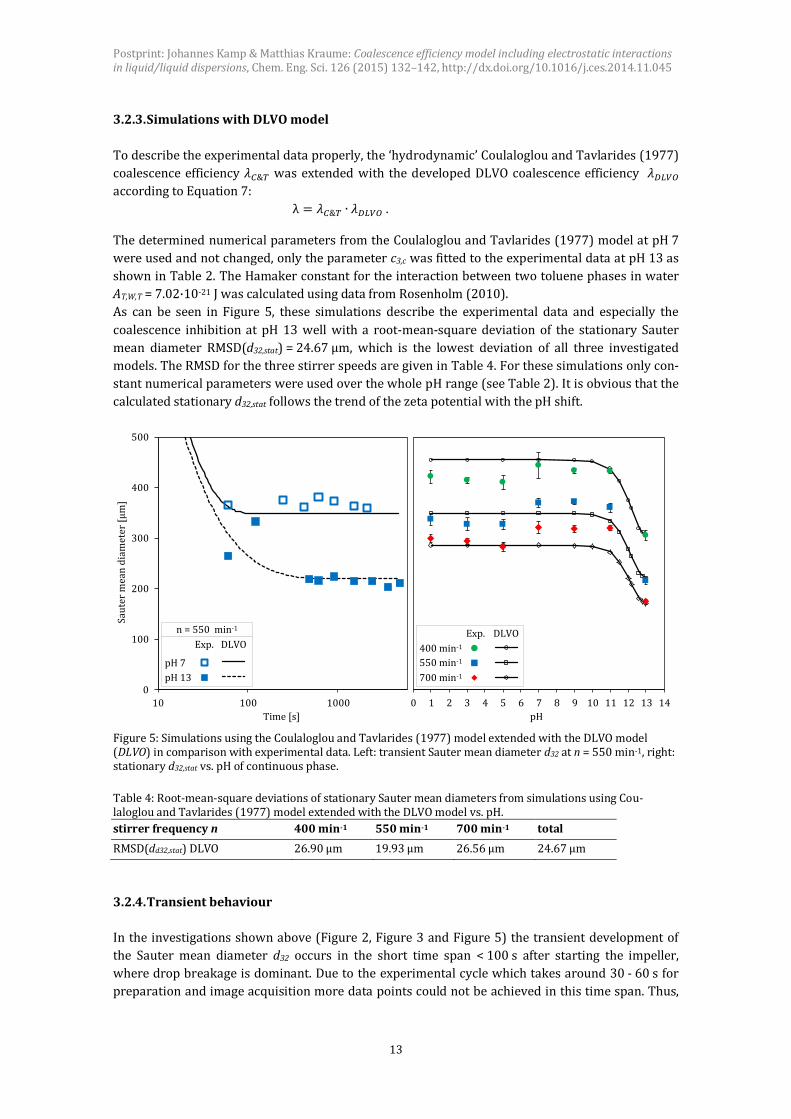
3.2.3. Simulations with DLVO model
To describe the experimental data properly, the ‘hydrodynamic’ Coulaloglou and Tavlarides (1977)
coalescence efficiency 𝜆𝐶&𝑇 was extended with the developed DLVO coalescence efficiency 𝜆𝐷𝐿𝑉𝑂
according to Equation 7:
λ = 𝜆𝐶&𝑇 ∙ 𝜆𝐷𝐿𝑉𝑂 .
The determined numerical parameters from the Coulaloglou and Tavlarides (1977) model at pH 7
were used and not changed, only the parameter c3,c was fitted to the experimental data at pH 13 as
shown in Table 2. The Hamaker constant for the interaction between two toluene phases in water
AT,W,T = 7.02·10-21 J was calculated using data from Rosenholm (2010).
As can be seen in Figure 5, these simulations describe the experimental data and especially the
coalescence inhibition at pH 13 well with a root-mean-square deviation of the stationary Sauter
mean diameter RMSD(d32,stat) = 24.67 μm, which is the lowest deviation of all three investigated
models. The RMSD for the three stirrer speeds are given in Table 4. For these simulations only con-
stant numerical parameters were used over the whole pH range (see Table 2). It is obvious that the
calculated stationary d32,stat follows the trend of the zeta potential with the pH shift.
Figure 5: Simulations using the Coulaloglou and Tavlarides (1977) model extended with the DLVO model (DLVO) in comparison with experimental data. Left: transient Sauter mean diameter d32 at n = 550 min-1, right: stationary d32,stat vs. pH of continuous phase.
Table 4: Root-mean-square deviations of stationary Sauter mean diameters from simulations using Cou-laloglou and Tavlarides (1977) model extended with the DLVO model vs. pH.
stirrer frequency n 400 min-1 550 min-1 700 min-1 total
RMSD(dd32,stat) DLVO 26.90 μm 19.93 μm 26.56 μm 24.67 μm
3.2.4. Transient behaviour
In the investigations shown above (Figure 2, Figure 3 and Figure 5) the transient development of
the Sauter mean diameter d32 occurs in the short time span < 100 s after starting the impeller,
where drop breakage is dominant. Due to the experimental cycle which takes around 30 - 60 s for
preparation and image acquisition more data points could not be achieved in this time span. Thus,
0
100
200
300
400
500
10 100 1000 0 1 2 3 4 5 6 7 8 9 10 11 12 13 14
Time [s] pH
Sau
ter
mea
n d
iam
eter
[μ
m]
0
100
200
300
400
500
10 1000
550rpm pH 7
550rpm pH13
sim pH7
sim pH13
0
100
200
300
400
500
10 1000
550rpm pH 7
550rpm pH13
sim pH7
sim pH13
Exp. DLVO
pH 7
pH 13
Exp. DLVO
400 min-1
01234567891011121314
400 rpm
550 rpm
700 rpm
sim400 pH1-11
sim550 pH1-11
sim700 pH1-11
sim400 pH11-13
sim550 pH11-13
sim700 pH11-13
01234567891011121314
400 rpm
550 rpm
700 rpm
sim400 pH1-11
sim550 pH1-11
sim700 pH1-11
sim400 pH11-13
sim550 pH11-13
sim700 pH11-13
550 min-1
700 min-1
n = 550 min-1

Postprint: Johannes Kamp & Matthias Kraume: Coalescence efficiency model including electrostatic interactions in liquid/liquid dispersions, Chem. Eng. Sci. 126 (2015) 132–142, http://dx.doi.org/10.1016/j.ces.2014.11.045
14
the standard procedure to investigate the transient behaviour of a system is to change the stirrer
frequency stepwise in an experiment. Particularly the coalescence behaviour can be examined if the
stirrer speed is decreased abruptly after a steady state has been reached. This was investigated in
experiments by changing the stirrer frequency from n = 700 min-1 to 400 min-1 and simulated with
the given numerical parameters (see Table 2) to analyse the transient behaviour of the three coa-
lescence efficiency sub models. In Figure 6 the results are shown for pH 13, where coalescence is
inhibited and the transient development of the drop size is well observable.
Figure 6: Transient development of the Sauter mean diameter d32 at pH 13 with a change in stirrer frequency n from 700 min-1 to 400 min-1 after 80 min in experiments and simulations using the three coalescence efficiency sub models (C&T: Coulaloglou and Tavlarides (1977), T&R: Tobin and Ramkrishna (1999), DLVO: hydrody-namic model from Coulaloglou and Tavlarides (1977) extended with DLVO model).
In the first part of this experiment with a stirrer frequency of n = 700 min-1 no significant transient
behaviour can be observed experimentally because drop breakage occurs fast in this system and
obviously is the dominant phenomenon after starting the impeller. The steady state is reached after
a few minutes. This is described adequately by all three sub models as discussed above, whereas
the Coulaloglou and Tavlarides (1977) model differs in the steady state and the transient behaviour
of the Tobin and Ramkrishna (1999) model is too slow. After 80 minutes when the stirrer frequen-
cy was changed to n = 400 min-1 coalescence predominates breakage and the Sauter mean diameter
d32 increases during the following 10 minutes until a steady state is reached again. The stationary
Sauter mean diameter d32,stat is equal to the one achieved starting with n = 400 min-1 (compare to
Figure 2, Figure 3 and Figure 5 right hand side at pH 13). The only coalescence efficiency model
describing this transient behaviour well is the Coulaloglou and Tavlarides (1977) model extended
with the DLVO model. The sole Coulaloglou and Tavlarides (1977) model overestimates the coales-
cence rate and therefore predicts a too fast transient development of the Sauter mean diameter. In
contrast, the Tobin and Ramkrishna (1999) model underestimates the coalescence rate and the
increase of d32 cannot be described properly.
3.2.5. Drop size distributions
The Sauter mean diameter d32 is an important quantity to evaluate the drop size distribution in
technical applications with one numerical value, nevertheless the underlying drop size distribution
Time [s]
Sau
ter
mea
n d
iam
eter
[μ
m]
100
150
200
250
300
350
0 1000 2000 3000 4000 5000 6000 7000
Exp.
400 min-1
01234567891011121314
400 rpm
550 rpm
700 rpm
sim400 pH1-11
sim550 pH1-11
sim700 pH1-11
sim400 pH11-13
sim550 pH11-13
sim700 pH11-13
700 min-1
01234567891011121314
400 rpm
550 rpm
700 rpm
sim400 pH1-11
sim550 pH1-11
sim700 pH1-11
sim400 pH11-13
sim550 pH11-13
sim700 pH11-13
C&T T&R DLVO
100
150
200
250
300
350
0200040006000
FBM pH13 700rpm
FBM pH13 400rpm
exp pH13 700rpm
exp pH13 400rpm
C&T pH13 700rpm
C&T pH13 400rpm
T&R pH13 700rpm
T&R pH13 400rpm
100
150
200
250
300
350
0200040006000
FBM pH13 700rpm
FBM pH13 400rpm
exp pH13 700rpm
exp pH13 400rpm
C&T pH13 700rpm
C&T pH13 400rpm
T&R pH13 700rpm
T&R pH13 400rpm
100
150
200
250
300
350
0200040006000
FBM pH13 700rpm
FBM pH13 400rpm
exp pH13 700rpm
exp pH13 400rpm
C&T pH13 700rpm
C&T pH13 400rpm
T&R pH13 700rpm
T&R pH13 400rpm
pH 13
n = 700 min-1 n = 400 min-1
Postprint: Johannes Kamp & Matthias Kraume: Coalescence efficiency model including electrostatic interactions in liquid/liquid dispersions, Chem. Eng. Sci. 126 (2015) 132–142, http://dx.doi.org/10.1016/j.ces.2014.11.045
15
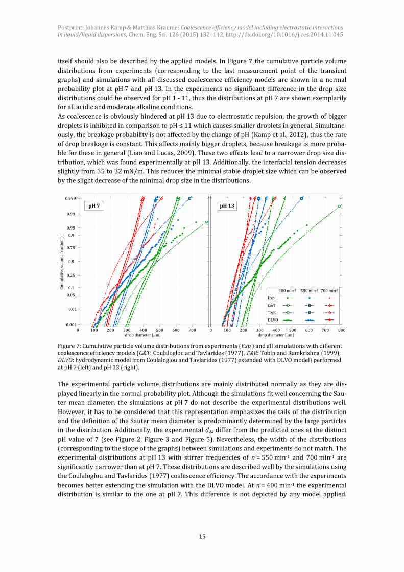
itself should also be described by the applied models. In Figure 7 the cumulative particle volume
distributions from experiments (corresponding to the last measurement point of the transient
graphs) and simulations with all discussed coalescence efficiency models are shown in a normal
probability plot at pH 7 and pH 13. In the experiments no significant difference in the drop size
distributions could be observed for pH 1 - 11, thus the distributions at pH 7 are shown exemplarily
for all acidic and moderate alkaline conditions.
As coalescence is obviously hindered at pH 13 due to electrostatic repulsion, the growth of bigger
droplets is inhibited in comparison to pH ≤ 11 which causes smaller droplets in general. Simultane-
ously, the breakage probability is not affected by the change of pH (Kamp et al., 2012), thus the rate
of drop breakage is constant. This affects mainly bigger droplets, because breakage is more proba-
ble for these in general (Liao and Lucas, 2009). These two effects lead to a narrower drop size dis-
tribution, which was found experimentally at pH 13. Additionally, the interfacial tension decreases
slightly from 35 to 32 mN/m. This reduces the minimal stable droplet size which can be observed
by the slight decrease of the minimal drop size in the distributions.
Figure 7: Cumulative particle volume distributions from experiments (Exp.) and all simulations with different coalescence efficiency models (C&T: Coulaloglou and Tavlarides (1977), T&R: Tobin and Ramkrishna (1999), DLVO: hydrodynamic model from Coulaloglou and Tavlarides (1977) extended with DLVO model) performed at pH 7 (left) and pH 13 (right).
The experimental particle volume distributions are mainly distributed normally as they are dis-
played linearly in the normal probability plot. Although the simulations fit well concerning the Sau-
ter mean diameter, the simulations at pH 7 do not describe the experimental distributions well.
However, it has to be considered that this representation emphasizes the tails of the distribution
and the definition of the Sauter mean diameter is predominantly determined by the large particles
in the distribution. Additionally, the experimental d32 differ from the predicted ones at the distinct
pH value of 7 (see Figure 2, Figure 3 and Figure 5). Nevertheless, the width of the distributions
(corresponding to the slope of the graphs) between simulations and experiments do not match. The
experimental distributions at pH 13 with stirrer frequencies of n = 550 min-1 and 700 min-1 are
significantly narrower than at pH 7. These distributions are described well by the simulations using
the Coulaloglou and Tavlarides (1977) coalescence efficiency. The accordance with the experiments
becomes better extending the simulation with the DLVO model. At n = 400 min-1 the experimental
distribution is similar to the one at pH 7. This difference is not depicted by any model applied.
0 100 200 300 400 500 600 700 800
0.001
0.01
0.05
0.1
0.25
0.5
0.75
0.9
0.95
0.99
0.999
0 100 200 300 400 500 600 700 800
0.001
0.01
0.05
0.1
0.25
0.5
0.75
0.9
0.95
0.99
0.999
drop diameter [m]
Cu
mu
lati
ve
vo
lum
e fr
acti
on
[-]
Probability plot for Normal distribution Q3 @ pH7
0 100 200 300 400 500 600 700 800
0.001
0.01
0.05
0.1
0.25
0.5
0.75
0.9
0.95
0.99
0.999
0 100 200 300 400 500 600 700 800
0.001
0.01
0.05
0.1
0.25
0.5
0.75
0.9
0.95
0.99
0.999
drop diameter [m]
Cu
mu
lati
ve
pro
bab
ilit
y [
-]Probability plot for Normal distribution Q3 @ pH13
400 min-1 550 min-1 700 min-1
C&T
T&R
DLVO
Exp.
0 100 200 300 400 500 600 700 800
0.001
0.01
0.05
0.1
0.25
0.5
0.75
0.9
0.95
0.99
0.999
C&T 400rpm
C&T 550rpm
C&T 700rpm
T&R 400rpm
T&R 550rpm
T&R 700rpm
FBM 400rpm
FBM 550rpm
FBM 700rpm
Exp. 400rpm
Exp. 550rpm
Exp. 700rpm
0 100 200 300 400 500 600 700 800
0.001
0.01
0.05
0.1
0.25
0.5
0.75
0.9
0.95
0.99
0.999
drop diameter [m]
Cu
mu
lati
ve
pro
bab
ilit
y [
-]
Probability plot for Normal distribution Q3 @ pH13
0 100 200 300 400 500 600 700 800
0.001
0.01
0.05
0.1
0.25
0.5
0.75
0.9
0.95
0.99
0.999
C&T 400rpm
C&T 550rpm
C&T 700rpm
T&R 400rpm
T&R 550rpm
T&R 700rpm
FBM 400rpm
FBM 550rpm
FBM 700rpm
Exp. 400rpm
Exp. 550rpm
Exp. 700rpm
0 100 200 300 400 500 600 700 800
0.001
0.01
0.05
0.1
0.25
0.5
0.75
0.9
0.95
0.99
0.999
drop diameter [m]
Cu
mu
lati
ve
pro
bab
ilit
y [
-]Probability plot for Normal distribution Q3 @ pH13
0 100 200 300 400 500 600 700 800
0.001
0.01
0.05
0.1
0.25
0.5
0.75
0.9
0.95
0.99
0.999
C&T 400rpm
C&T 550rpm
C&T 700rpm
T&R 400rpm
T&R 550rpm
T&R 700rpm
FBM 400rpm
FBM 550rpm
FBM 700rpm
Exp. 400rpm
Exp. 550rpm
Exp. 700rpm
0 100 200 300 400 500 600 700 800
0.001
0.01
0.05
0.1
0.25
0.5
0.75
0.9
0.95
0.99
0.999
drop diameter [m]
Cu
mu
lati
ve
pro
bab
ilit
y [
-]
Probability plot for Normal distribution Q3 @ pH13
0 100 200 300 400 500 600 700 800
0.001
0.01
0.05
0.1
0.25
0.5
0.75
0.9
0.95
0.99
0.999
C&T 400rpm
C&T 550rpm
C&T 700rpm
T&R 400rpm
T&R 550rpm
T&R 700rpm
FBM 400rpm
FBM 550rpm
FBM 700rpm
Exp. 400rpm
Exp. 550rpm
Exp. 700rpm
0 100 200 300 400 500 600 700 800
0.001
0.01
0.05
0.1
0.25
0.5
0.75
0.9
0.95
0.99
0.999
drop diameter [m]
Cu
mu
lati
ve
pro
bab
ilit
y [
-]
Probability plot for Normal distribution Q3 @ pH13
pH 7 pH 13
Postprint: Johannes Kamp & Matthias Kraume: Coalescence efficiency model including electrostatic interactions in liquid/liquid dispersions, Chem. Eng. Sci. 126 (2015) 132–142, http://dx.doi.org/10.1016/j.ces.2014.11.045
16
Throughout most system conditions the model of Tobin and Ramkrishna (1999) shows the largest
deviations from the experimental distributions.
The narrow distributions in the simulations are mainly determined by the daughter drop size dis-
tribution of the breakage kernel. Due to mass balance conservation a relatively narrow normal
distribution was applied (see section 2.3). A broader daughter drop size distribution would lead to
broader distributions in the simulations but also result in a significant loss of mass during simula-
tion. Using an advanced daughter drop size distribution based on single drop breakage investiga-
tions, Maaß et al. (2007) showed that the broad experimental distributions can be predicted well.
As the focus in this work lies on the coalescence modelling, the breakage kernel was kept as basic as
possible and confined to the Coulaloglou and Tavlarides (1977) model.
4. Summary and outlook
The presented implementation of the DLVO theory into population balance equations offers the
possibility to extend hydrodynamic models of coalescence efficiency so that the coalescence inhibi-
tion due to electrostatic effects can be described effectively. This was applied for drop size distribu-
tion measurements in a stirred tank with NaOH, NaCl and HCl present and an ionic strength of
I = 0.1 mol/L. The coalescence inhibition at high pH values was modelled successfully extending the
model of Coulaloglou and Tavlarides (1977) with the developed DLVO model using only constant
numerical parameters. The gained results are able to describe the steady state and transient exper-
imental data better than the models of Coulaloglou and Tavlarides (1977) or Tobin and Ramkrishna
(1999), where a parameter variation is inevitable to describe the pH dependency of the Sauter
mean diameter.
The surface potential has to be known, but may be approximated with the zeta potential. As the
type of oil has a minor influence on the pH dependency of the zeta potential, the presented model
can be adapted to several investigations available in literature (e.g. Creux et al. (2009), Gray-Weale
and Beattie (2009) and Marinova et al. (1996)) for different salts and conditions. If proper data is
not available, the zeta potential can be measured and its pH dependency can be described with
Stern adsorption isotherm and Grahame equation as presented in this work.
In integral applications of the population balance equation trajectories of single droplets and there-
fore distances between drops are not available. Hence, the Debye length is defined as the character-
istic distance between the drops to calculate the attractive van der Waals and the repulsive electro-
static force.
An interesting further improvement of this DLVO model could be a general description of the pH
dependency of the zeta potential for varying ionic strength and the implementation of other ionic
species. Additionally, the model equations could be extended to describe also the presence of mul-
tivalent ions.
Acknowledgements
The authors kindly thank Mirco Wegener for providing the experimental data and the student
workers Elies Espí Novell and Jin Zoo Lee who substantially contributed to this work. Moreover, the
authors kindly thank the Institute of Soft Matter and Functional Materials at Helmholtz Zentrum
Berlin for providing the possibility of measuring the zeta potential. Financial support provided by
the German Research Foundation (DFG) within the project KR 1639/19-1 is gratefully acknowl-
edged.

Postprint: Johannes Kamp & Matthias Kraume: Coalescence efficiency model including electrostatic interactions in liquid/liquid dispersions, Chem. Eng. Sci. 126 (2015) 132–142, http://dx.doi.org/10.1016/j.ces.2014.11.045
17
Nomenclature
Latin letters
a curvature (here: droplet) radius [m]
a numerical parameter in isotherm fit [V]
A1,2,3 Hamaker constant [J]
b numerical parameter in isotherm fit [-]
c numerical parameter in isotherm fit [V]
c1,b numerical parameter in PBE: breakage rate [-]
c2,b numerical parameter in PBE: breakage rate [-]
c1,c numerical parameter in PBE: collision frequency [-]
c2,c numerical parameter in PBE: ‘hydrodynamic’ coalescence efficiency various
c3,c numerical parameter in PBE: ‘electrostatic’ coalescence efficiency various
d stirrer diameter [m]
d32 Sauter mean diameter [m]
dp particle / droplet diameter [m]
dp,max maximal particle / droplet diameter [m]
dμ mean value of drop size distribution [m]
dσ standard deviation of drop size distribution [m]
D tank diameter [m]
e elementary charge: 1.6022∙10-19 C [C]
𝑓 number density function [m-3]
fϵ prefactor of energy dissipation rate [-]
Fel electrostatic double layer force [N]
FvdW van der Waals force [N]
F force [N]
g breakage rate [s-1]
h droplet distance [m]
H tank height [m]
I ionic strength [mol/L]
kB Boltzmann constant: 1.3806∙10-23 J/K [J/K]
n stirrer frequency [min-1]
nd number of daughter drops after breakage event: 2 [-]
ni,0 number concentration of ion i in bulk [m-3]
nsalts,0 number concentration of all salts in bulk [m-3]
NA Avogadro constant: 6.0221∙1023 mol-1 [mol-1]
pH decimal logarithm of the reciprocal hydrogen ion activity [-]
Req equivalent droplet radius [m]
RMSD(𝑋) root-mean-square deviation of quantity X various
t time [s]
T temperature [K]
ue electrophoretic mobility [m2/(V∙s)]

Postprint: Johannes Kamp & Matthias Kraume: Coalescence efficiency model including electrostatic interactions in liquid/liquid dispersions, Chem. Eng. Sci. 126 (2015) 132–142, http://dx.doi.org/10.1016/j.ces.2014.11.045
18
Vp particle / droplet volume [m3]
Vμ mean value of daughter drop volume distribution [m3]
Vσ standard deviation of daughter drop volume distribution [m3]
𝑋𝑖 experimental value various
�̂�𝑖 calculated value various
zi valence / charge number of ion i [-]
Greek letters
β daughter drop size distribution [-]
ϵ energy dissipation rate [m2/s3]
εr relative permittivity [-]
ε0 vacuum permittivity: 8.8542∙10-12 F/m [F/m]
γ interfacial tension [N/m]
inverse Debye length [m-1]
λ coalescence efficiency / probability [-]
Γi number concentration of ion i at surface / interface [m-2]
Γ0 reference saturation adsorption at surface / interface [m-2]
i volume of hydrated ion i [m3]
φ phase fraction [-]
Φi specific interaction energy of ion i [J]
Ψs surface potential [V]
σ surface charge density [C/m2]
θi surface coverage of ion i [-]
𝜉 collision frequency [m3/s]
ζ zeta potential [V]
Abbreviations
C&T Coulaloglou and Tavlarides (1977)
DLVO Derjaguin, Landau, Verwey & Overbeek theory
PBE Population balance equation(s)
PTFE Polytetrafluoroethylene
RMSD root-mean-square deviation
T&R Tobin and Ramkrishna (1999)
Literature
Attarakih, M.M., Bart, H.-J., Faqir, N.M., 2004. Numerical solution of the spatially distributed population balance equation describing the hydrodynamics of interacting liquid–liquid dispersions. Chem. Eng. Sci. 59, 2567–2592. http://dx.doi.org/10.1016/j.ces.2004.03.005
Beattie, J.K., Djerdjev, A.M., 2004. The Pristine Oil/Water Interface: Surfactant-Free Hydroxide-Charged Emulsions. Angew. Chemie 116, 3652–3655. http://dx.doi.org/10.1002/ange.200453916
Beattie, J.K., Djerdjev, A.M., Franks, G. V, Warr, G.G., 2005. Dipolar Anions Are Not Preferentially Attracted to the Oil/Water Interface. J. Phys. Chem. B 109, 15675–15676. http://dx.doi.org/10.1021/jp052894l
Postprint: Johannes Kamp & Matthias Kraume: Coalescence efficiency model including electrostatic interactions in liquid/liquid dispersions, Chem. Eng. Sci. 126 (2015) 132–142, http://dx.doi.org/10.1016/j.ces.2014.11.045
19
Beattie, J.K., Gray-Weale, A., 2012. Oil/Water Interface Charged by Hydroxide Ions and Deprotonated Fatty Acids: A Comment. Angew. Chemie Int. Ed. 51, 12941–12942. http://dx.doi.org/10.1002/anie.201205927
Butt, H.-J., Graf, K., Kappl, M., 2003. Physics and Chemistry of Interfaces (Physics Textbook). Wiley-VCH, Weinheim. http://dx.doi.org/10.1002/3527602313
Carroll, B.J., 1976. The stability of emulsions and mechnisms of emulsion breakdown, in: Matijevic, E. (Ed.), Surface and Colloid Science. Wiley-Interscience, New York, pp. 1–68.
Chibowski, E., Wiacek, A.E., Holysz, L., Terpilowski, K., 2005. Investigation of the electrokinetic properties of paraffin suspension. 1. In inorganic electrolyte solutions. Langmuir 21, 4347–4355. http://dx.doi.org/10.1021/la046921v
Coulaloglou, C.A., Tavlarides, L.L., 1977. Description of interaction processes in agitated liquid-liquid dispersions. Chem. Eng. Sci. 32, 1289–1297. http://dx.doi.org/10.1016/0009-2509(77)85023-9
Creux, P., Lachaise, J., Graciaa, A., Beattie, J.K., Djerdjev, A.M., 2009. Strong Specific Hydroxide Ion Binding at the Pristine Oil/Water and Air/Water Interfaces. J. Phys. Chem. B 113, 14146–14150. http://dx.doi.org/10.1021/jp906978v
David, F., Vokhminz, V., Ionova, G., 2001. Water Characteristics Depend on the Ionic Environment. Thermodynamics and Modelisation of the Aquo Ions. J. Mol. Liq. 90, 45–62. http://dx.doi.org/10.1016/S0167-7322(01)00106-4
Delgado, A. V, González-Caballero, F., Hunter, R.J., Koopal, L.K., 2007. Measurement and interpretation of electrokinetic phenomena. J. Colloid Interface Sci. 309, 194–224. http://dx.doi.org/10.1016/j.jcis.2006.12.075
Derjaguin, B., 1934. Untersuchungen über die Reibung und Adhäsion, IV. Kolloid-Zeitschrift 69, 155–164. (in German). http://dx.doi.org/10.1007/bf01433225
Derjaguin, B. V, 1989. Theory of Stability of Colloids and Thin Films. Consultants Bureau, New York.
Derjaguin, B. V, Churaev, N. V, Muller, V.M., 1987. Surface Forces. Consultants Bureau, New York.
Derjaguin, B. V, Landau, E.M., 1941. Theory of the stability of strongly charged lyophobic sols and of the adhesion of strongly charged particles in solutions of electrolytes. Acta Physicochitnica U.R.S.S. 14, 633–662. (reprint: Progress in Surface Science, 1993 (43), 30–59, http://dx.doi.org/10.1016/0079-6816(93)90013-L). http://dx.doi.org/10.1016/0079-6816(93)90013-L
Dunstan, D.E., 1992. The Electrophoretic Mobility of Hydrocarbon Particles in KCl Solutions. Langmuir 8, 1507–1508. http://dx.doi.org/10.1021/la00042a002
Franks, G. V, Djerdjev, A.M., Beattie, J.K., 2005. Absence of Specific Cation or Anion Effects at Low Salt Concentrations on the Charge at the Oil/Water Interface. Langmuir 21, 8670–8674. http://dx.doi.org/10.1021/la051379b
Gäbler, A., 2007. Experimentelle Untersuchungen, Modellierung und Simulation gerührter Flüssig/flüssig-Systeme mit veränderlichen Stoff- und Betriebsparametern. PhD Thesis, Technische Universität Berlin, Fachgebiet Verfahrenstechnik. (in German)
Gäbler, A., Wegener, M., Paschedag, A.R., Kraume, M., 2006. The effect of pH on experimental and simulation results of transient drop size distributions in stirred liquid-liquid dispersions. Chem. Eng. Sci. 61, 3018–3024. http://dx.doi.org/10.1016/j.ces.2005.10.072
Gray-Weale, A., Beattie, J.K., 2009. An explanation for the charge on water’s surface. Phys. Chem. Chem. Phys. 11, 10994. http://dx.doi.org/10.1039/b901806a
Hamaker, H.C., 1937. The London-Van der Vaals attraction between spherical particles. Phys. IV 10, 1058–1072. http://dx.doi.org/10.1016/S0031-8914(37)80203-7
Hulburt, H.M., Katz, S., 1964. Some problems in particle technology. Chem. Eng. Sci. 19, 555–574. http://dx.doi.org/10.1016/0009-2509(64)85047-8
Israelachvili, J.N., 1991. Intermolecular and Surface Forces, 2nd ed. Academic Press, London.
Izutsu, K., 2002. Electrochemistry in Nonaqueous Solutions. Wiley-VCH, Weinheim.

Postprint: Johannes Kamp & Matthias Kraume: Coalescence efficiency model including electrostatic interactions in liquid/liquid dispersions, Chem. Eng. Sci. 126 (2015) 132–142, http://dx.doi.org/10.1016/j.ces.2014.11.045
20
Jou, F.-Y., Mather, A.E., 2003. Liquid-Liquid Equilibria for Binary Mixtures of Water + Benzene, Water + Toluene, and Water + p -Xylene from 273 K to 458 K. J. Chem. Eng. Data 48, 750–752. http://dx.doi.org/10.1021/je034033g
Kamp, J., Nachtigall, S., Maaß, S., Kraume, M., 2012. Modelling of coalescence in turbulent liquid/liquid dispersions considering droplet charge. Czas. Tech. Mech. Politech. Krak. 109, 113–124. (Errata in: http://www.verfahrenstechnik.tu-berlin.de/fileadmin/fg158/Dokumente/Manuskripte/2012/Kamp_CTM_2012_Manuskript.pdf)
Kopriwa, N., Buchbender, F., Ayesteran, J., Kalem, M., Pfennig, A., 2012. A Critical Review of the Application of Drop-Population Balances for the Design of Solvent Extraction Columns: I. Concept of Solving Drop-Population Balances and Modelling Breakage and Coalescence. Solvent Extr. Ion Exch. 30, 683–723. http://dx.doi.org/10.1080/07366299.2012.700598
Kraume, M., Gäbler, A., Schulze, K., 2004. Influence of physical properties on drop size distributions of stirred liquid-liquid dispersions. Chem. Eng. Technol. 27, 330–334. http://dx.doi.org/10.1002/ceat.200402006
Liao, Y., Lucas, D., 2009. A literature review of theoretical models for drop and bubble breakup in turbulent dispersions. Chem. Eng. Sci. 64, 3389–3406. http://dx.doi.org/10.1016/j.ces.2009.04.026
Liao, Y., Lucas, D., 2010. A literature review on mechanisms and models for the coalescence process of fluid particles. Chem. Eng. Sci. 65, 2851–2864. http://dx.doi.org/10.1016/j.ces.2010.02.020
Lyklema, J., 2000. Fundamentals of Interface and Colloid Science Vol. III: Liquid-fluid interfaces, Fundamentals of Interface and Colloid Science. Academic Press, London.
Maaß, S., Gäbler, A., Zaccone, A., Paschedag, A.R., Kraume, M., 2007. Experimental Investigations and Modelling of Breakage Phenomena in Stirred Liquid/Liquid Systems. Chem. Eng. Res. Des. 85, 703–709. http://dx.doi.org/10.1205/cherd06187
Maaß, S., Wollny, S., Voigt, A., Kraume, M., 2011. Experimental comparison of measurement techniques for drop size distributions in liquid/liquid dispersions. Exp. Fluids 50, 259–269. http://dx.doi.org/10.1007/s00348-010-0918-9
Marinova, K.G., Alargova, R.G., Denkov, N.D., Velev, O.D., Petsev, D.N., Ivanov, I.B., Borwankar, R.P., 1996. Charging of Oil-Water Interfaces Due to Spontaneous Adsorption of Hydroxyl Ions. Langmuir 12, 2045–2051. http://dx.doi.org/10.1021/la950928i
Miller, C.A., Neogi, P., 2008. Interfacial phenomena: equilibrium and dynamic effects, Surfactant science series. CRC Press, Taylor & Francis, Boca Raton, FL.
Overbeek, J.T.G., 1952. Electrochemistry of the double layer, in: Kruyt, H.R. (Ed.), Colloid Science: Irreversible Systems. Elsevier, Amsterdam, pp. 115–193.
Pfennig, A., Schwerin, A., 1998. Influence of Electrolytes on Liquid-Liquid Extraction. Ind. Eng. Chem. Res. 37, 3180–3188. http://dx.doi.org/10.1021/ie970866m
Rambhau, D., 1978. Zeta potential: a force that monitors dispersion stability. Indian J. Pharm. Educ. 12, 140–151.
Rambhau, D., Phadke, D.S., Dorle, A.K., 1977. Evaluation of o/w emulsion stability through zeta potential. I. J. Soc. Cosmet. Chem. 28, 183–196.
Ramkrishna, D., 1985. Status of population balances. Rev. Chem. Eng. 3, 49–95. http://dx.doi.org/10.1515/REVCE.1985.3.1.49
Ramkrishna, D., 2000. Population Balances: Theory and Applications to Particulate Systems in Engineering. Academic Press, San Diego.
Randolph, A.D., Larson, M.A., 1962. Transient and steady state size distributions in continuous mixed suspension crystallizers. AIChE J. 8, 639–645. http://dx.doi.org/10.1002/aic.690080515
Ritter, J., Kraume, M., 2000. On-line Measurement Technique for Drop Size Distributions in Liquid/Liquid Systems at High Dispersed Phase Fractions. Chem. Eng. Technol. 23, 579–581. http://dx.doi.org/10.1002/1521-4125(200007)23:7<579::AID-CEAT579>3.0.CO;2-Y
Roger, K., Cabane, B., 2012a. Why Are Hydrophobic/Water Interfaces Negatively Charged? Angew. Chemie Int. Ed. 51, 5625–5628. http://dx.doi.org/10.1002/anie.201108228
Postprint: Johannes Kamp & Matthias Kraume: Coalescence efficiency model including electrostatic interactions in liquid/liquid dispersions, Chem. Eng. Sci. 126 (2015) 132–142, http://dx.doi.org/10.1016/j.ces.2014.11.045
21
Roger, K., Cabane, B., 2012b. Uncontaminated Hydrophobic/Water Interfaces Are Uncharged: A Reply. Angew. Chemie 124, 13117–13119. http://dx.doi.org/10.1002/ange.201207114
Rosenholm, J.B., 2010. Critical comparison of molecular mixing and interaction models for liquids, solutions and mixtures. Adv. Colloid Interface Sci. 156, 14–34. http://dx.doi.org/10.1016/j.cis.2010.02.005
Smoluchowski, M., 1903. Contribution à la théorie l´endosmose électrique et de quelques phénomènes corrélatifs. Bull. Int. l’Académie des Sci. Cracovie, Cl. des Sci. Mathématiques Nat. 182–199. (in French)
Stern, O., 1924. Zur Theorie der elektrolytischen Doppelschicht. Z. Elektrochem. Angew. Phys. Chem. 30, 508–516. (in German). http://dx.doi.org/10.1002/bbpc.192400182
Tian, C.S., Shen, Y.R., 2009. Structure and charging of hydrophobic material/water interfaces studied by phase-sensitive sum-frequency vibrational spectroscopy. Proc. Natl. Acad. Sci. 106, 15148–15153. http://dx.doi.org/10.1073/pnas.0901480106
Tobin, T., Ramkrishna, D., 1992. Coalescence of charged droplets in agitated liquid-liquid dispersions. AIChE J. 38, 1199–1205. http://dx.doi.org/10.1002/aic.690380807
Tobin, T., Ramkrishna, D., 1999. Modeling the effect of drop charge on coalescence in turbulent liquid-liquid dispersions. Can. J. Chem. Eng. 77, 1090–1104. http://dx.doi.org/10.1002/cjce.5450770603
Tsonopoulos, C., 2001. Thermodynamic analysis of the mutual solubilities of hydrocarbons and water. Fluid Phase Equilib. 186, 185–206. http://dx.doi.org/10.1016/S0378-3812(01)00520-9
Vacha, R., Rick, S.W., Jungwirth, P., de Beer, A.G.F., de Aguiar, H.B., Samson, J.-S., Roke, S., 2011. The Orientation and Charge of Water at the Hydrophobic Oil Droplet-Water Interface. J. Am. Chem. Soc. 133, 10204–10210. http://dx.doi.org/10.1021/ja202081x
Verwey, E.J.W., Overbeek, J.T.G., 1948. Theory of the Stability of Lyophobic Colloids. Elsevier, New York.
Villwock, J., Gebauer, F., Kamp, J., Bart, H.-J., Kraume, M., 2014. Systematic Analysis of Single Droplet Coalescence. Chem. Eng. Technol. 37, 1103–1111. http://dx.doi.org/10.1002/ceat.201400180
Wagner, K., Friese, T., Schulz, S., Ulbig, P., 1998. Solubilities of Sodium Chloride in Organic and Aqueous-Organic Solvent Mixtures. J. Chem. Eng. Data 43, 871–875. http://dx.doi.org/10.1021/je9800510
Wang, T., Wang, J., Jin, Y., 2003. A novel theoretical breakup kernel function for bubbles/droplets in a turbulent flow. Chem. Eng. Sci. 58, 4629–4637. http://dx.doi.org/10.1016/j.ces.2003.07.009
Watanabe, A., 1984. Electrochemistry of oil-water interfaces, in: Matijevic, E. (Ed.), Surface and Colloid Science. Wiley-Interscience, New York, pp. 1–70.
Wegener, M., 2004. Experimentelle Untersuchungen und Modellierung von transienten Tropfengrößenverteilungen in gerührten Flüssig-flüssig-Systemen. Master Thesis, Chair of Chemical and Process Engineering, Technische Universität Berlin. (in German)
Wulkow, M., Gerstlauer, A., Nieken, U., 2001. Modeling and simulation of crystallization processes using parsival. Chem. Eng. Sci. 56, 2575–2588. http://dx.doi.org/10.1016/S0009-2509(00)00432-2
Zaccone, A., Gäbler, A., Maaß, S., Marchisio, D., Kraume, M., 2007. Drop breakage in liquid/liquid stirred dispersions: Modelling of single drop breakage. Chem. Eng. Sci. 62, 6297–6307. http://dx.doi.org/10.1016/j.ces.2007.07.026
Top Related