


Languages
Pages
Legal


Portland State University Portland State University
PDXScholar PDXScholar
Environmental Science and Management Faculty Publications and Presentations Environmental Science and Management
9-2015
Climate-Suitable Planting as a Strategy for Climate-Suitable Planting as a Strategy for
Maintaining Forest Productivity and Functional Maintaining Forest Productivity and Functional
Diversity Diversity
Matthew Joshua Duveneck Portland State University
Robert M. Scheller Portland State University, [email protected]
Follow this and additional works at: https://pdxscholar.library.pdx.edu/esm_fac
Part of the Ecology and Evolutionary Biology Commons, Environmental Sciences Commons, and the
Forest Biology Commons
Let us know how access to this document benefits you.
Citation Details Citation Details Matthew J. Duveneck and Robert M. Scheller 2015. Climate-suitable planting as a strategy for maintaining forest productivity and functional diversity. Ecological Applications 25:1653–1668.
This Article is brought to you for free and open access. It has been accepted for inclusion in Environmental Science and Management Faculty Publications and Presentations by an authorized administrator of PDXScholar. Please contact us if we can make this document more accessible: [email protected].

Ecological Applications, 25(6), 2015, pp. 1653–1668� 2015 by the Ecological Society of America
Climate-suitable planting as a strategy for maintaining forestproductivity and functional diversity
MATTHEW J. DUVENECK1
AND ROBERT M. SCHELLER
Department of Environmental Science and Management, Portland State University, Portland, Oregon 97201 USA
Abstract. Within the time frame of the longevity of tree species, climate change willchange faster than the ability of natural tree migration. Migration lags may result in reducedproductivity and reduced diversity in forests under current management and climate change.We evaluated the efficacy of planting climate-suitable tree species (CSP), those tree specieswith current or historic distributions immediately south of a focal landscape, to maintain orincrease aboveground biomass, productivity, and species and functional diversity. Wemodeled forest change with the LANDIS-II forest simulation model for 100 years (2000–2100)at a 2-ha cell resolution and five-year time steps within two landscapes in the Great Lakesregion (northeastern Minnesota and northern lower Michigan, USA). We compared currentclimate to low- and high-emission futures. We simulated a low-emission climate future withthe Intergovernmental Panel on Climate Change (IPCC) 2007 B1 emission scenario and theParallel Climate Model Global Circulation Model (GCM). We simulated a high-emissionclimate future with the IPCC A1FI emission scenario and the Geophysical Fluid DynamicsLaboratory (GFDL) GCM. We compared current forest management practices (business-as-usual) to CSP management. In the CSP scenario, we simulated a target planting of 5.28% and4.97% of forested area per five-year time step in the Minnesota and Michigan landscapes,respectively. We found that simulated CSP species successfully established in both landscapesunder all climate scenarios. The presence of CSP species generally increased simulatedaboveground biomass. Species diversity increased due to CSP; however, the effect onfunctional diversity was variable. Because the planted species were functionally similar tomany native species, CSP did not result in a consistent increase nor decrease in functionaldiversity. These results provide an assessment of the potential efficacy and limitations of CSPmanagement. These results have management implications for sites where diversity andproductivity are expected to decline. Future efforts to restore a specific species or forest typemay not be possible, but CSP may sustain a more general ecosystem service (e.g., abovegroundbiomass).
Key words: annual net primary productivity; assisted migration; carbon emission scenarios; climate-suitable planting; forest simulation modeling; functional diversity; Great Lakes region, USA; LANDIS-IImodel; managed relocation.
INTRODUCTION
Forest management for future climate conditions
must accept and use new paradigms for continued
success in delivering ecosystem services (e.g., carbon
sequestration, biodiversity, biomass, and wildlife habi-
tat). Restoration of forest species composition to a
historical range of variability (HRV; Landres et al. 1999,
Wiens et al. 2012) may not be a realistic goal (Hobbs et
al. 2011). Despite adaptation strategies to manage for
resilience (Seidl et al. 2011, Duveneck et al. 2014a),
extant tree species may not be suitable for future
establishment, given their climate tolerances.
Within the next century, many tree species may not be
capable of naturally migrating to more suitable sites at
the rate of the changing climate (Scheller and Mladenoff
2008, Loarie et al. 2009, Bradshaw et al. 2010, Zhu et al.
2012, Diffenbaugh and Field 2013, Svenning and Sandel
2013). Even if suitable species are present or arrive in
low abundance, a temporal lag is expected between
arrival and expansion (Bradshaw and Lindbladh 2005,
Wangen and Webster 2006, Birks and Birks 2008).
Although this lag may not result in regional extirpation,
the site or landscape may experience a decline in the
density of extant species associated with a decline in
ecosystem services. There is growing interest to explore
climate suitable planting (CSP), also referred to as
‘‘assisted migration,’’ ‘‘assisted colonization,’’ or ‘‘man-
aged relocation,’’ whereby tree species are planted
beyond their current range (Marris 2009, Richardson et
al. 2009, Pedlar et al. 2012, Schwartz et al. 2012). This
alternative management prescription is designed to
facilitate migration while maintaining forest function,
e.g., species diversity and carbon sequestration (Millar
et al. 2007, O’Neill et al. 2008b). Given the lack of
Manuscript received 17 April 2014; revised 8 December 2014;accepted 11 December 2014. Corresponding Editor: C. H. Sieg.
1 E-mail: [email protected]
1653

experimental work focused on climate suitable planting,
landscape modeling provides a suitable framework to
assess the ability of CSP to overcome spatial and
temporal migration barriers in forested ecosystems
(Rehfeldt et al. 2006, Campbell et al. 2009).
Climate-suitable planting
If future climate conditions reduce species and forest
type diversity, the adaptive capacity of ecosystems will
be compromised. Fewer species will reduce the response
capability of forests to changing environmental condi-
tions (Walker 1992, Walker et al. 1999). Low-diversity
forests are also more susceptible to single-host insect or
disease outbreaks (Naeem and Li 1997, Bentz et al.
2010). Increasing or maintaining diversity in these
forests may create more climate-change-resilient forests
(Chapin et al. 2007). This may be done by intensively
planting a climate-suitable species following a distur-
bance when an undesirable condition such as lower
productivity is otherwise expected (Spittlehouse and
Stewart 2003).
Successful planting and establishment of a desired
native species may become increasingly difficult as
climate changes (Ledig and Kitzmiller 1992), making
species from outside the range of a site more desirable
(O’Neill et al. 2008b, Gray et al. 2010). In order to
consider CSP management, it is vital to consider the
biotic interactions of novel ecosystems, ecosystems
composed of new species compositions (Blois et al.
2013). Assessing how these species might replace native
niche spaces and/or expand their own niche space will
provide a framework to evaluate the efficacy of CSP.
Rather than assisted migration for the refuge of a
threatened species, maintaining a high level of function
within a site or region requires new terminology and
frameworks for success (Pedlar et al. 2012). A CSP
prescription is designed to maintain or increase the
ecosystem services of a site, e.g., biodiversity, carbon
storage, timber products (Millar et al. 2007, O’Neill et
al. 2008a). These objectives are different from the
interest to protect or save an endangered species (Barlow
and Martin 2004, Hoegh-Guldberg et al. 2008, Lunt et
al. 2013). Assisted migration proposals for the protec-
tion of rare and endangered species are fraught with
controversy, including a concern about negative effects
if a species becomes invasive (Barlow and Martin 2004,
McLachlan et al. 2007, Davidson and Simkanin 2008,
Ricciardi and Simberloff 2009). Others however, have
described potential benefits of nonnative species. These
benefits include providing functional substitutes for
declining or extinct native species (Schlaepfer et al.
2011). For example, within managed or degraded
forests, CSP may be one of the only options for
maintaining ecosystem services (Lunt et al. 2013).
The agriculture community has a growing recognition
of species suitability shifts, as evidenced by the
difference between the 1990 and 2012 plant hardiness
maps (Daly et al. 2012). For silviculturists, this concept
is familiar. Many commercial tree seedlings come from
nursery stock grown in different regions of the country
from where they are planted. Seedlings are selected
based on the suitability matched to site conditions.
Given the longevity of tree species, forest managers are
seeking information about future suitability of seedlings.
Online climate envelope models such as the ‘‘Seedlot
Selection Tool,’’ while not a simulation model, have
been developed to assist managers to find seedlots for
selected sites based on projected future conditions
(available online).2 In addition, this tool can select
planting sites that are appropriate for particular
seedlots. Because climate change uncertainty is high
(IPCC 2013), simulation modeling of CSP is considered
a vital component to understanding potential outcomes
and choosing management alternatives regarding CSP
(Perez et al. 2012, Breed et al. 2013).
Species and functional diversity
Species diversity is recognized as having a strong tie to
potential ecosystem services (Tilman et al. 2006, Duve-
neck et al. 2014b). In addition, functional diversity (FD)
based on functional traits has proven to be a useful
measure of diversity. Rather than individual species, FD
is based on the range of ecological functions provided by
a community (Cornelissen et al. 2003, Laliberte and
Legendre 2010). There is strong evidence that FD is a
driver to ecosystem services (Dıaz et al. 2007, Mokany et
al. 2008) and ecosystem resilience (Folke et al. 2004),
defined as ‘‘the capacity of a system to absorb
disturbance and reorganize while undergoing change
so as to retain essentially the same function’’ (Folke et
al. 2004:558).
Our objectives were to assess the efficacy of CSP to
increase aboveground biomass (AGB), aboveground
annual net primary productivity (ANPP), and species
and functional diversity of forests expected to be
substantially affected by climate change. Our previous
work assessed business-as-usual (BAU) management
under climate change (Duveneck et al. 2014b), and how
modified forest management would compare to BAU
(Duveneck et al. 2014a). In this work, we addressed the
following questions. (1) As an alternative to business-as-
usual (BAU) management, how might CSP under
climate change affect AGB and ANPP? (2) How might
CSP affect functional and species diversity under climate
change as a surrogate for future ecosystem services?
We examined these questions within two landscapes in
the upper Great Lakes of Minnesota and Michigan.
These landscapes provided large variation in climate,
soils, and forest management (Duveneck et al. 2014b).
Northeastern Minnesota and northern lower Michigan
landscapes provide island-like landscapes nearly sur-
rounded by a combination of lakes, lowland conifer
2 http://sst.forestry.oregonstate.edu/
MATTHEW J. DUVENECK AND ROBERT M. SCHELLER1654 Ecological ApplicationsVol. 25, No. 6

forests, and agricultural development along the boreal–
temperate forest ecotone (Curtis 1959).
METHODS
Study area
We selected two landscapes in the northern Great
Lakes region within the boreal–temperate transition zone
(i.e., northeastern Minnesota and northern lower Mich-
igan; Fig. 1). Our landscapes encompass approximately
1.6 and 2.6 million ha of forest in the Minnesota and
Michigan landscapes, respectively. We chose this region
because the climate (IPCC 2013, Staudinger et al. 2013)
and forests (Fisichelli et al. 2013, Duveneck et al. 2014b,
Handler et al. 2014a, b) are expected to change substan-
tially. By the end of the 21st century, temperatures in the
region are expected to increase by 3–118C (Andresen et al.
2012). In addition, these landscapes are naturally
bounded by fragmentation, large bodies of water, and
boreal–swamp forests (to the north of northeastern
Minnesota), creating island-like conditions. For these
reasons, we expect new species moving into these
landscapes to be limited. We leveraged previous work in
the region to parameterize natural disturbance regimes,
initial species composition conditions, and BAU silvicul-
ture prescriptions (Duveneck et al. 2014b).
Simulation model and experimental design
Our experimental design included both BAU and CSP
management. For each management scenario, we
assessed three climate scenarios. For all simulations,
we used a 100-year time horizon starting at year 2000
and 2-ha cell resolution. We used a 2-ha cell size to
balance forest composition precision with the computa-
tional processing time required of the simulations. In
order to make our results more comparable to prior
research in the region, whenever possible, we used
consistent methodology between this study and prior
research (Duveneck et al. 2014a, b).
We modeled forest change using the LANDIS-II v6.0
forest landscape model at five-year time steps (Scheller et
al. 2007). LANDIS-II is a spatially explicit landscape
change model. Driven by ecological processes,
LANDIS-II can be run at multiple temporal and spatial
scales, and has been widely used (Gustafson et al. 2010,
Ravenscroft et al. 2010, Thompson et al. 2011).
Processes within the LANDIS-II modeling framework
include tree species establishment, growth, mortality,
and seed dispersal; fire; wind; and timber harvesting.
These processes interact spatially and functionally
across interconnected cells within climate and soil
regions on a landscape.
We used the PnET-II tool for LANDIS-II (Xu et al.
2009) to calculate species-specific parameters, i.e.,
maximum aboveground net primary productivity per
year (ANPPmax) and probability of establishment (Pest).
These parameters are a function of climate (temperature,
precipitation, and photosynthetic active radiation
(PAR)) along with soil water-holding capacity (SWHC)
and species-specific physiological parameters (e.g., foliar
nitrogen content and maximum foliar mass area). We
employed the PnET-II tool for each unique climate–soil
region (Duveneck et al. 2014b).
LANDIS-II is built around a core modeling structure.
The core interacts with user-chosen extensions of varying
complexity. We used the LANDIS-II Biomass Succession
extension (v3.1), which regulates the succession mecha-
nisms of growth, reproductive maturity, and age-related
mortality for species-cohorts (Scheller and Mladenoff
2004). Because Biomass Succession does not include
density or diameter information, natural mortality due to
stand development is a function of age, whereby cohort
thinning leads to a decline in biomass and growth
capacity over time. Although age is not a perfect proxy
FIG. 1. Landscape study areas in northeastern Minnesota and northern lower Michigan, USA.
September 2015 1655CLIMATE-SUITABLE PLANTING AS STRATEGY

for thinning, it sufficiently captures the general patterns
over large landscapes (Scheller and Mladenoff 2004).
The PnET-II output parameters ANPPmax and Pest
are utilized directly by the Biomass Succession exten-
sion. ANPPmax regulates the maximum growth possible
of aboveground biomass for a species-cohort (Scheller
and Mladenoff 2004); Pest determines the probability of
a new cohort establishing, given a local seed source and
adequate light (Xu et al. 2009).
We also simulated harvesting, fire, and wind distur-
bances. We used the Biomass Harvest extension (v2.1) to
simulate harvest and planting prescriptions (Gustafson
et al. 2000, Syphard et al. 2011). We applied specific
prescriptions to unique management areas, described
previously (Duveneck et al. 2014b). These management
areas are based on ownership groups (i.e., state, county,
U.S. Forest Service, private industrial, private non-
industrial, and forest reserve areas). We delineated
harvest stands within each management area to repre-
sent the range and variability of current stands within
specific forest types. For each five-year time step,
multiple unique prescriptions were implemented. First,
the Biomass Harvest extension selected stands for
treatment based on a stand ranking customized for each
forest type. Next, biomass was harvested from cells
within stands based on prescription-specific criteria.
Prescription-specific rotation periods within each man-
agement area defined the proportion of the management
area to be treated at each time step (Gustafson et al.
2000). Proportion to be treated within each management
area was based on current proportion of forest types
allowing for up to a 30% increase in area harvested if
simulated future forest types matched harvest prescrip-
tions. When CSP species matured to merchantable age,
we harvested them with existing northern hardwood and
oak prescriptions. We simulated natural fire and wind
disturbance utilizing the Base Fire (v3.0; He and
Mladenoff 1999) and Base Wind (v2.0; Scheller and
Mladenoff 2004) extensions. Given uncertainty in future
projections of natural disturbances (e.g., Butler et al.
2012) and the interest in reducing experimental varia-
tion, we simulated fire and wind disturbances based on
recent trends rather than dynamic variation in future
disturbance regimes. To quantify spatially explicit
species aboveground biomass (AGB), we used the
Biomass Output extension (v2.0). We utilized previously
developed initial communities, fire and wind regimes,
BAU timber harvest regimes, delineated ecoregions, and
PnET-II parameters (Duveneck et al. 2014b).
Climate data
For each unique climate region (described in Duve-
neck et al. 2014b), we accessed downscaled monthly
climate data through the USGS data portal (Stoner et
al. [2012]; available online).3 We simulated current
climate by randomly assigning observed monthly
PRISM climate data (1969–1999) to future simulation
years (Daly and Gibson 2002). We simulated climate
change with future projections for years 2000–2100.
We simulated a low-emission climate future with the
IPCC B1 emission scenario (IPCC 2007) and the
Parallel Climate Model (PCM) Global Circulation
Model (GCM) (Washington et al. 2000). We simulated
a high-emission climate future with the IPCC A1FI
emission scenario (IPCC 2007) and the Geophysical
Fluid Dynamics Laboratory (GFDL) GCM (Delworth
et al. 2006). Climate projections from the PCM GCM
are considered less sensitive to emissions than the
GFDL GCM. The combination of carbon emission
scenarios with GCM sensitivity will hereafter be
referred to as low- and high-emission scenarios (Fig.
2). We bracketed a large range of plausible futures by
coupling the separate emission scenarios to the more
and less sensitive GCMs. In addition, these GCM
emission scenario combinations are being used in
other research in the region, providing model projec-
tion consistency (Peters et al. 2013, Handler et al.
2014a, b).
Climate-suitable planting
We simulated planting tree species expected to
respond well to a warmer climate. For each landscape,
we selected three tree species that were present,
according to range distribution maps (Burns and
Honkala 1990), within 250 km south of each landscape
boundary but were absent or in low abundance within
each landscape; and whose habitat suitability are
expected to increase with climate change (Iverson et al.
2008). For our CSP species selection, we leveraged
previous habitat suitability analysis completed in north-
ern Minnesota (Handler et al. 2014a) and northern
lower Michigan (Handler et al. 2014b). Habitat suitabil-
ity was assessed using a climate envelope approach
where future temperature, future precipitation, topog-
raphy, and soils were used to model future suitable
habitat based on present species distribution (Iverson et
al. 2008). In northeastern Minnesota, we selected
bitternut hickory (Carya cordiformis), black oak (Quer-
cus velutina), and northern pin oak (Quercus ellipsoida-
lis). In northern lower Michigan, we selected bitternut
hickory, shagbark hickory (Carya ovata), and scarlet
oak (Quercus coccinea).
In addition to the three selected species, we simulated
planting American chestnut (Castanea dentata) in each
landscape. American chestnut once was widespread
throughout the mid-Atlantic United States (Russell
1987). The introduction of the chestnut blight (Crypho-
nectria parasitica) wiped out mature American chestnut
throughout its range (Keever 1953, Lovett et al. 2006,
Jacobs et al. 2013). Prior to the blight infection,
American chestnut was considered a foundation species
that had a strong role in structuring the forest
community. Given the auspicious properties of Ameri-3 http://cida.usgs.gov/climate/gdp/
MATTHEW J. DUVENECK AND ROBERT M. SCHELLER1656 Ecological ApplicationsVol. 25, No. 6

can chestnut, there has been considerable interest and
investment in restoring the species with a blight-resistant
hybrid (Smith 2000) that will likely be available in the
near future (American Chestnut Foundation 2013).
Although additional southern species are expected to
have climate-suitable habitat in our landscapes (Iverson
et al. 2008), we limited our experimental design to four
species in each landscape.
The CSP prescriptions were implemented within
existing harvesting regimes and management areas
(Duveneck et al. 2014b). CSP prescriptions were only
simulated in actively managed forests, excluding reserve
areas such as the Boundary Waters Canoe Area
Wilderness in Minnesota. Specifically, we simulated
CSP wherever patch-cutting harvesting occurred in
northern hardwood stands. Compared to BAU manage-
ment, we simulated a fourfold frequency increase in
implementing the northern hardwoods patch-cutting
prescription for the first 50 simulation years. The planting
intensity resulted in a target planting of 5.28% and 4.97%
of forested area per five-year time step in the Minnesota
and Michigan landscapes, respectively. This equates to
planting ;17 111 and 22 180 ha/yr in the Minnesota and
Michigan landscapes, respectively. We chose this planting
intensity to balance a plausible management scenario
(e.g., The Nature Conservancy planted 800 ha of climate-
suitable seedlings in northeastern Minnesota in 2013 (M.
White, personal communication), with a simulation
experiment that was deliberately intensive. Because we
simulated species-cohorts rather than individual seed-
lings, we did not simulate a specific planting density of
seedlings within a site or stand.
Species and functional diversity
As a measure of species diversity, we calculated the
Shannon Index of diversity, H0 (Gotelli and Ellison
2004). We calculated H0 within each landscape, utilizing
species abundance (i.e., simulated AGB of individual
tree species). We transformed H0 to the effective number
of species (eH0
) as the number of species present if all
species were equal in abundance. This transformation
reduces inaccuracies when comparing diversity between
scenarios (Jost 2006).
We calculated functional diversity within each land-
scape with the functional dispersion (FDis) index
(Laliberte and Legendre 2010). Rather than counting
species or groups of species, FDis is based on user-
defined a priori traits (Villeger et al. 2008, Laliberte and
Legendre 2010). For example, two separate species with
identical user-defined traits would contribute the same
FDis as one species. By definition, individual species are
different from one another. Therefore, FDis is valuable
when traits are considered that affect potential ecosys-
tem functions of interest, e.g., nutrient cycling, carbon
storage, carbon sequestration, and wildlife habitat
(Cornelissen et al. 2003).
Specifically, FDis is the weighted (by abundance) mean
distance of species traits in multidimensional space to the
centroid of all species (Anderson et al. 2006). FDis is a
flexible FD framework allowing both quantitative and
qualitative traits, more traits than species, and the ability
to weigh individual traits. FDis is not strongly influenced
by outliers because it takes into account relative
abundance (Laliberte and Legendre 2010). To calculate
FDis, abundance was represented as simulated tree
FIG. 2. Projected July maximum temperature and annual precipitation in each landscape and emission scenario for the years2000 to 2100.
September 2015 1657CLIMATE-SUITABLE PLANTING AS STRATEGY

species AGB. We utilized a species trait matrix used in
previous research (Paquette and Messier 2011) and added
species to the trait matrix that were unique to our study.
Specific species traits included maximum height, growth
rate, leaf size, longevity, foliar mass per area, foliar
nitrogen content, wood density, decay resistance, vegeta-
tive reproduction, seed mass, pollination vector, mycor-
rhizal infection type, shade tolerance, drought tolerance,
and water-logging tolerance (Tables 1 and 2).
Analysis
We compared aboveground ANPP and diversity of
BAU management to CSP management under each
climate scenario. We calculated eH0
and FDis diversity
for every cell in a simulation and created raster files for
each diversity index and scenario. We used these layers
of diversity and LANDIS-II ANPP output raster layers
for further spatial analysis. Of the actively managed
cells, we separated sites where CSP species were present
vs. absent to compare ANPP. We used the vegan-
community ecology (Oksanen et al. 2012), FD function-
al diversity (Laliberte and Legendre 2010), and raster
(Hijmans and Etten 2013) libraries in R (R Core Team
2013) for all calculations and analysis.
We replicated each simulation five times in order to
examine the stochastic variation within scenarios. The
model stochastic behavior was largely driven by natural
disturbances of fire and wind. The within-scenario
variation was small due to the low stochastic variation
of natural disturbance events relative to the large size of
the landscapes. As an attempt to increase result
variation, we bootstrapped the five replicates 1000 times
under our three climate futures and two management
scenarios. Given the low number of replicates (due to
long computational time), the variance from the boot-
strapping did not increase substantially. Compared to
the total AGB replicate mean at year 2100, the
maximum variance was less than 0.05% for every
individual replicate. Therefore, we randomly selected
one replicate from each simulation for additional
analysis. Although strict validation of future simulation
results is not possible, species-specific parameters used in
PnET-II and the Biomass Succession extension to
LANDIS-II have been evaluated in other northern
Great Lakes landscapes (Scheller and Mladenoff 2004,
Xu et al. 2007, Ravenscroft et al. 2010). Furthermore,
we evaluated LANDIS-II simulated AGB to U.S. Forest
Service Forest Inventory and Analysis field plot
TABLE 1. Some species traits used to calculate FDis (Paquette and Messier 2011).
Species H (m) GR LS WD (g/m3) WDR SeM (mg) LL (months) LMA (g/m2) N (%)
Abies balsamea 25 1 1 0.34 1 2.15 4.70 151.00 1.66Acer rubrum 25 3 3 0.49 1 3.04 1.72 71.09 1.91Acer saccharum 35 1 3 0.56 1 4.19 1.71 70.63 1.83Betula alleghaniensis 25 3 2 0.55 1 0.70 1.71 46.08 2.20Betula papyrifera 25 3 2 0.48 1 0.29 1.28 77.88 2.31Carya cordiformis 25 1 4 0.60 1 7.98 1.61 44.05 2.60Carya ovata 35 1 4 0.64 1 8.39 1.61 75.00 1.76Castanea dentate 30 3 3 0.40 3 8.15 1.61 100.00 2.30Fagus grandifolia� 25 1 2 0.56 1 5.66 1.61 61.22 2.04Fraxinus americana 30 2 4 0.55 1 3.83 1.74 76.75 2.12Fraxinus nigra 20 2 4 0.45 1 4.08 1.61 71.94 2.10Fraxinus pennsylvanica 25 3 4 0.53 1 3.50 1.61 87.72 1.80Picea glauca 25 1 1 0.35 1 1.15 3.91 302.86 1.28Picea mariana 20 1 1 0.41 1 0.74 3.81 294.12 1.12Pinus banksiana 20 3 5 0.42 1 1.50 3.30 243.90 1.24Pinus resinosa 25 3 5 0.39 1 2.27 3.58 294.12 1.17Pinus strobus 30 3 5 0.36 2 2.89 3.00 121.92 1.42Pinus sylvestris� 21 3 5 0.42 1 1.79 3.30 243.90 1.24Populus balsamifera� 25 3 2 0.37 1 0.26 1.28 83.46 1.95Populus grandidentata 20 3 2 0.39 1 0.17 1.61 70.45 2.50Populus tremuloides 25 3 2 0.37 1 0.14 1.58 82.02 2.16Prunus serotina 22 3 2 0.47 3 4.55 1.71 72.30 2.48Quercus alba 35 1 3 0.60 3 8.17 1.61 81.21 2.39Quercus coccinea 30 3 3 0.60 3 7.57 1.61 95.00 1.90Quercus ellipsoidalis 22 1 3 0.56 3 8.50 1.79 88.00 2.29Quercus macrocarpa� 15 1 3 0.58 3 8.71 1.79 92.74 2.27Quercus rubra 25 2 3 0.56 2 8.20 1.79 84.20 2.06Quercus velutina� 18 2 3 0.56 3 8.50 1.79 98.00 2.40Thuja occidentalis 15 1 1 0.30 3 0.83 3.50 223.00 1.02Tilia americana 35 2 3 0.32 1 2.77 1.61 60.81 2.94Tsuga canadensis 30 1 1 0.40 1 2.31 4.09 122.55 0.99Ulmus americana 35 3 3 0.46 1 2.00 1.78 79.47 2.07
Note: Terms are H, average maximum height; GR, growth rate (1, slow; 2, moderate; 3, rapid); LS, leaf size (1, needle/scale; 2,small ,10 cm; 3, large; 4, compound; WD, wood density (specific gravity); WDR, wood decay resistance (1, not; 2, moderate; 3,resistant; 4, very resistant); SeM, seed mass; LL, leaf longevity; LMA, leaf mass per area; N, nitrogen content per leaf mass unit.
� Michigan landscape only.� Minnesota landscape only.
MATTHEW J. DUVENECK AND ROBERT M. SCHELLER1658 Ecological ApplicationsVol. 25, No. 6

estimates of AGB in northern lower Michigan (Pear-
son’s correlation of 0.64, and RMSE of 44.3 Mg/ha).
Details of our biomass evaluation are described in
Duveneck et al. (2014b).
RESULTS
Aboveground biomass and annual net primary
productivity
The high-emission climate scenario resulted in sub-
stantially less simulated total and harvested AGB
compared to current and low-emission climate scenarios
by year 2100 (Fig. 3). The large increase in simulated
AGB under current and low emissions is a reflection of
continued AGB recovery following large-scale logging
across the region in the early 20th century. CSP
management resulted in greater simulated total AGB
compared to BAU management (Fig. 3). In the
Minnesota landscape, simulated AGB at year 2100
increased under the CSP scenario by 18%, 19%, and 30%
in the current, low-emission, and high-emission climate
scenarios, respectively. In the Michigan landscape,
where greater total AGB was simulated in general,
AGB at year 2100 increased less under the CSP scenario
(3%, 3%, and 7% in the current, low-emission, and high-
emission climate scenarios, respectively). In the Minne-
sota landscape, CSP under each climate scenario
resulted in greater total AGB compared to BAU. In
the Michigan landscape, larger AGB due to CSP was
most pronounced under the high-emission climate
scenario. Harvested AGB followed a pattern similar to
that of total AGB. Harvested AGB was greater under
CSP, but there was an overall declining trend in
harvested AGB under the high-emission scenario. As
simulated planted species matured to a merchantable
age, more simulated biomass was harvested compared to
BAU management (Fig. 3B). The initial larger harvested
CSP biomass in the Minnesota landscape is due to an
increase in implementation frequency of the northern
hardwoods patch-cutting prescription necessary to
implement the CSP treatment.
In each simulated landscape, CSP species established
and increased in AGB through time (Fig. 4). The current
and low-emission climate scenario generally resulted in
greater CSP species AGB compared to the high-emission
climate scenario. The Michigan landscape exhibited
TABLE 2. Additional species traits used to calculate FDis (Paquette and Messier 2011).
Species Veg Pa Pb TolS TolD TolW AM EM
Abies balsamea 1 1 0 5.0 1.0 2.0 0 1Acer rubrum 1 1 1 3.4 1.8 3.1 1 0Acer saccharum 1 1 1 4.8 2.3 1.1 1 0Betula alleghaniensis 1 1 0 3.2 3.0 2.0 0 1Betula papyrifera 1 1 0 1.5 2.0 1.3 0 1Carya cordiformis 0 1 0 2.1 4.0 2.5 0 1Carya ovata 2 1 0 3.4 3.0 1.4 0 1Castanea dentata 2 1 0 3.1 3.0 1.0 0 1Fagus grandifolia� 2 1 0 4.8 1.5 1.5 0 1Fraxinus americana 1 1 0 2.5 2.4 2.6 1 0Fraxinus nigra 1 1 0 3.0 2.0 3.5 1 0Fraxinus pennsylvanica 1 1 0 3.1 3.9 3.0 1 0Picea glauca 0 1 0 4.2 2.9 1.0 0 1Picea mariana 2 1 0 4.1 2.0 2.0 0 1Pinus banksiana 0 1 0 1.4 4.0 1.0 0 1Pinus resinosa 0 1 0 1.9 3.0 1.0 0 1Pinus strobus 0 1 0 3.2 2.3 1.0 0 1Pinus sylvestris� 0 1 0 1.4 4.0 1.0 0 1Populus balsamifera� 1 1 0 1.3 1.8 2.6 1 1Populus grandidentata 1 1 0 1.2 2.5 2.0 1 1Populus tremuloides 1 1 0 1.2 1.8 1.8 1 1Prunus serotina 0 0 1 2.5 3.0 1.1 1 1Quercus alba 0 1 0 2.9 3.6 1.4 0 1Quercus coccinea 2 1 0 2.1 4.0 1.0 0 1Quercus ellipsoidalis 2 1 0 2.9 2.9 1.2 0 1Quercus macrocarpa� 0 1 0 2.7 3.9 1.8 0 1Quercus rubra 1 1 0 2.8 2.9 1.1 0 1Quercus velutina� 1 1 0 2.8 3.9 1.2 0 1Thuja occidentalis 2 1 0 3.5 2.7 1.5 1 0Tilia americana 1 0 1 4.0 2.9 1.3 0 1Tsuga canadensis 0 1 0 4.8 1.0 1.3 0 1Ulmus americana 1 1 0 3.1 2.9 2.5 1 0
Note: Terms are Veg, vegetative reproduction (0, never; 1, possible; 2, common); Pa, abioticpollination (0, not possible; 1, possible); Pb, biotic pollination (0, not possible; 1, possible); TolS,shade tolerance (1, intolerant; 5, tolerant); TolD, drought tolerance (1, intolerant; 5, tolerant);TolW, waterlogging tolerance (1, intolerant; 5, tolerant); AM, arbuscular mycorrhiza (0, notpossible; 1, possible); EM, ectomycorrhiza (0, not possible; 1, possible).
� Michigan landscape only.� Minnesota landscape only.
September 2015 1659CLIMATE-SUITABLE PLANTING AS STRATEGY

larger climate scenario effects and larger increases in
CSP species AGB compared to the Minnesota land-
scape. Of the planted species, American chestnut and
bitternut hickory resulted in the largest increases in
simulated AGB by year 2100.
Like AGB, aboveground ANPP was lower under the
high-emission scenario compared to the current and
low-emission scenario (Fig. 5). Although both land-
scapes resulted in similar ANPP at year 2100, the
Minnesota landscape started with higher ANPP, and
resulted in larger declines. Especially apparent in the
Michigan landscape under the high-emission climate
scenario, simulated ANPP resulted in a rapid decline
before year 2050, followed by a relatively stable period.
The stable period of ANPP may be due to the climate
becoming more suitable for certain native species. In
both landscapes, the effect of CSP resulted in limited
differences in simulated ANPP as compared to BAU
management. Specifically, simulated ANPP in the CSP
management scenario under the high-emission climate
scenario did not equal simulated ANPP under current
climate and BAU management.
Although AGB of CSP species increased less in the
high-emission scenario (Fig. 4), the proportion of cells
occupied by CSP species was greatest in the high-
emission scenario, followed by the low-emission and
current climate (Fig. 6A). Compared to actively
managed cells unoccupied by CSP species, actively
managed cells occupied by CSP species resulted in
similar simulated ANPP under the high-emission
scenario (Fig. 6B). The results of the current and low-
emission climate scenarios were mixed. Simulations in
the Minnesota landscape resulted in generally less
ANPP within CSP-occupied sites compared to unoccu-
pied CSP sites within the current and low-emission
climate scenario. After year 2070, the Michigan land-
scape resulted in greater simulated ANPP within CSP-
occupied sites compared to unoccupied CSP sites within
the current and low-emission climate scenario. The
initial lower simulated aboveground ANPP in CSP
species cells is expected due to the delayed growth in
young cohorts. As the initial planted species mature, the
effect of the growth lag in young cohort cells is reduced.
Species and functional diversity
The CSP scenario resulted in greater simulated species
diversity (eH0
). Larger species diversity due to CSP was
found in both landscapes under all climate scenarios and
time steps (Fig. 7). In the Minnesota landscape, the CSP
scenario also resulted in greater FDis in all climate
scenarios. The CSP scenario however, reached an
asymptote after 2050, while functional diversity under
the BAU scenario continued to increase. In the
Michigan landscape, where initial functional and species
FIG. 3. Simulated (A) total aboveground biomass (AGB) and (B) harvested AGB over the years 2000 to 2100 for eachlandscape, climate, and management scenario. BAU is business-as-usual management; CSP is climate-suitable plantingmanagement.
MATTHEW J. DUVENECK AND ROBERT M. SCHELLER1660 Ecological ApplicationsVol. 25, No. 6

diversity was higher, CSP resulted in less functional
diversity in all climate scenarios after 2030.
In the Minnesota landscape, the high-emission
climate scenario resulted in the largest increase in both
species and functional diversity. These results are in
contrast to the current and low-emission climate
scenarios, which resulted in a consistent, although
slower, increase in species diversity through time. The
Michigan landscape exhibited greater initial diversity
than Minnesota; over time, however, species diversity
declined. The Michigan landscape exhibited relatively
consistent FDis over time. The high- and low-emission
climate scenarios resulted in less species diversity than
current climate. The high-emission climate scenario,
however, resulted in the greatest functional diversity in
the Michigan landscape.
DISCUSSION
In some sites, CSP management may provide an
opportunity to increase ecosystem services such as AGB,
ANPP, and diversity under climate change. CSP may be
most effective in sites or landscapes when otherwise
large declines in productivity are expected (Stanturf et
al. 2014). At timescales in the range of the longevity of
many extant tree species (e.g., ,200 years), climate is
expected to change faster than species’ ability to
maintain equilibrium (Diffenbaugh and Field 2013,
Svenning and Sandel 2013). However, forest manage-
FIG. 4. Aboveground biomass (AGB) of climate-suitable planting species simulated in each landscape and climate scenario.American chestnut (Castanea dentata) and bitternut hickory (Carya cordiformis) were simulated in both landscapes. Other specieswere black oak (Quercus velutina), northern pin oak (Q. ellipsoidalis), scarlet oak (Q. coccinea), and shagbark hickory (Caryaobovata).
September 2015 1661CLIMATE-SUITABLE PLANTING AS STRATEGY
ment in our landscapes is often focused at rotation-
period time scales (i.e., ,100 years). The ability to
maintain forest ecosystem services at those timescales is
expected to be limited within traditional (Duveneck et
al. 2014b) and even alternative management (without the
use of CSP) (Duveneck et al. 2014a).
Aboveground biomass and annual net primary
productivity
As reported earlier (Duveneck et al. 2014b), under
high-emission climate, BAU management suggests less
simulated total and harvested AGB compared to
current and low-emission climate scenarios. Greater
simulated total and harvested ABG due to CSP
suggests that planting climate-suitable species may
increase the resilience of forests to the effects of climate
change. The larger CSP AGB results are small in
relation to the treatment intensity. Planting intensity
was 5.28% and 4.97% of each landscape at each five-
year time step in the Minnesota and Michigan
landscapes, respectively. This suggests that the CSP
scenario did not grossly contract the current niche
space used by extant tree species. Although the species
selected for planting are native to regions south of each
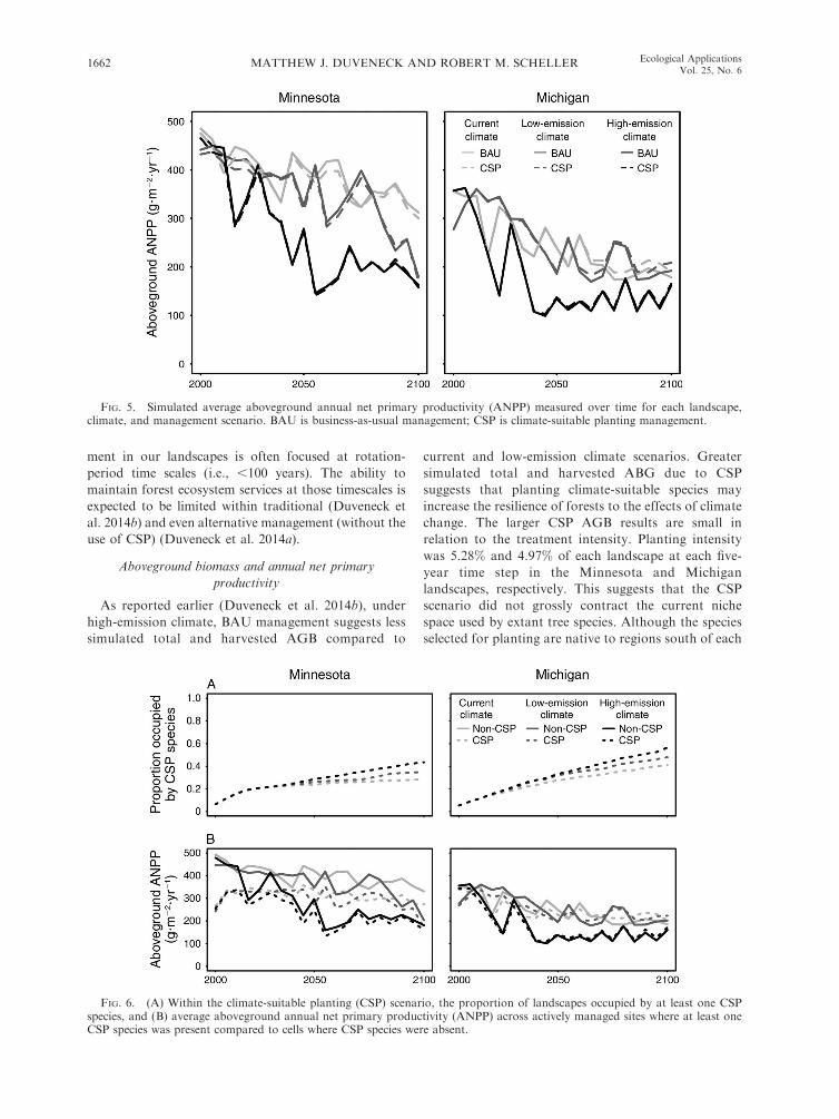
FIG. 5. Simulated average aboveground annual net primary productivity (ANPP) measured over time for each landscape,climate, and management scenario. BAU is business-as-usual management; CSP is climate-suitable planting management.
FIG. 6. (A) Within the climate-suitable planting (CSP) scenario, the proportion of landscapes occupied by at least one CSPspecies, and (B) average aboveground annual net primary productivity (ANPP) across actively managed sites where at least oneCSP species was present compared to cells where CSP species were absent.
MATTHEW J. DUVENECK AND ROBERT M. SCHELLER1662 Ecological ApplicationsVol. 25, No. 6

landscape, the high-emission climate scenario did not
result in the most optimized climate selection for those
species. The current and low-emission climate scenarios
resulted in more optimal growth as measured by
simulated AGB (Fig. 4). Had we simulated planting
species from even farther south, we expect to have
simulated more use of niche space, resulting in greater
increases in AGB and ANPP under the high-emission
climate.
The CSP treatment was implemented following
simulated patch-cutting harvests. The initial decline in
ANPP within CSP cells is due to the expected lag in
growth response of young cohorts (Bowler et al. 2012).
Compared to older stands, ANPP of recently harvested
sites would lag behind before increasing. Although the
non-CSP-occupied harvest areas (i.e., harvested stands
that did not include any CSP species) were also
vulnerable to disturbance, compared to the CSP sites,
which all started with a disturbance, the non-CSP sites
experienced less disturbance. Therefore, the majority of
non-CSP sites were mature stands. Nevertheless, average
ANPP within CSP sites was not substantially less than
non-CSP-occupied sites, despite continual harvesting
and new planting throughout the simulation. The CSP
scenario in the Michigan landscape under the current
and low-emission climate scenario resulted in greater
simulated ANPP than BAU after 2075 (Fig. 5). As
suggested in individual CSP species’ response to climate
(Fig. 4), the CSP species may have been best matched to
the current and low-emission climate scenarios in the
Michigan landscape.
In the Minnesota landscape, the net negative effect of
CSP on ANPP was greater in the current and low-
emission compared to the high-emission climate scenar-
io. Both the largest increase in proportion of sites
occupied by CSP species and the largest decline in AGB
and ANPP under BAU management were found under
the high-emission climate scenario. Under the high-
emission climate scenario, CSP species would have
replaced species declining under climate change, e.g.,
balsam fir (Abies balsamea) and black spruce (Picea
mariana), that would otherwise be abundant under
current climate (Duveneck et al. 2014b). This supports
the suggestion that CSP may be most appropriate where
large declines in productivity are expected (Lunt et al.
2013). Although the CSP scenario resulted in less of an
increase in AGB under high-emission climate compared
to current and low-emission climate, CSP did result in
greater total and harvested AGB under the high-
emission climate scenario where the largest BAU
declines were simulated (Fig. 3). This suggests a net
benefit in some ecosystem services under the CSP
scenario.
As a restoration species, recent research suggests that
American chestnut has the potential to fulfill much of its
historical role as a foundation species (Gauthier et al.
2013, Jacobs et al. 2013). As climate has changed and
will continue to change since American chestnut
dominated the canopy of Eastern forests (Andresen et
al. 2012), assessing landscape and site conditions for
habitat suitability will be vital for reintroduction
success. In the northern Great Lake region, disease-
resistant chestnut seedlings have been successfully
established within experimental plots (Jacobs and
Severeid 2004). Our results suggest that introduced
American chestnut has the potential to succeed within
regions north of its historic range.
FIG. 7. Average species diversity (eH0
) and functional diversity (FDis) across cells for each landscape, climate, and managementscenario over time. Light dotted lines represent standard error across cells for each scenario. BAU is business-as-usualmanagement; CSP is climate-suitable planting management.
September 2015 1663CLIMATE-SUITABLE PLANTING AS STRATEGY

Species and functional diversity
In the Michigan landscape, simulated diversityremained relatively constant compared to the Minnesota
landscape across all climate scenarios. This may be aresult of greater initial species and functional diversity.
In addition to inherent benefits of maintaining biodi-versity (e.g., more species are less vulnerable to single
host pathogens) (Wilson 2010), increasing diversity hasthe potential to enhance the range of environmental
tolerances of the ecosystems providing ecosystemservices (Walker 1992, Naeem and Li 1997). Within
lower-productivity sites, the relationship between diver-sity and productivity may become more important
(Loreau et al. 2001, Paquette and Messier 2011, Duve-neck et al. 2014b). Furthermore, under a high-emission
scenario, our results suggest productivity and AGBdeclines are expected.
CSP was more effective at increasing functionaldiversity in Minnesota than in Michigan. Where initial
species diversity was lower and decline in productivitywas higher (Minnesota), CSP initially resulted in greater
functional diversity compared to BAU management.Following 100 simulation years of high emissions,however, FDis under the BAU scenario nearly surpassed
FDis under the CSP scenario in the Minnesotalandscape, where initial FDis was lower. This may be
due to less initially dominant species (e.g., balsam fir andquaking aspen) under BAU because of a climate
mismatch (Duveneck et al. 2014b). As these speciesdeclined, the simulated response of less dominant species
became more equal, increasing FDis but decreasingAGB and ANPP. In addition, it is possible that the
increase in functional diversity under BAU relative toCSP simulations can also be attributed to non-CSP
species having unique functional roles that under CSPare being replaced by functionally similar CSP species.
Where initial species diversity was greater and thedecline in productivity was lower (Michigan), CSP
management resulted in less FDis compared to BAUmanagement. In theMichigan landscape, theCSP scenario
may have replaced functionally similar species, resulting ina landscape of less functionally dissimilar species. There-fore, landscapes expected to decline in productivity and
diversity may provide more opportunity for effectiveclimate management such as climate-suitable planting.
Because our diversity results reflect a 2-ha grain size, ourresults are not necessarily scalable to finer grain sizes
(Urban 2005). However, simulation results such as oursmay helpmanagers prioritize allocation of scarce resources
to areas more critically vulnerable than others.Given the novelty of assisted migration management
(Lawler and Olden 2011) and the social limits to change(Adger et al. 2009), we chose CSP species based on close
proximity (either current or historically) to our landscapes.This resulted in species that were functionally similar, i.e.,
functionally redundant (Walker 1992), to the speciesexpected to persist under climate change (i.e., northern
hardwoods and oaks). As such, CSP under the high-
emission climate did not maintain greater functional
diversity. Under BAU management and a high-emission
climate future, we expect less spruce–fir species in these
landscapes (Fisichelli et al. 2013, Duveneck et al. 2014b).
Had we simulated planting central Appalachian conifers
such as shortleaf pine (Pinus echinata), we would have
likely seen a greater and sustained increase in functional
diversity under climate change. Future work should
consider exploring CSP treatments based on function
replacement. Nevertheless, functional diversity generally
increased through time and was greatest under the high-
emission climate scenario in both landscapes (Fig. 7).
Management challenges to climate-suitable planting
The simulated benefits of CSP resulted from intensive
planting prescriptions. We did not address CSP effects
at varying management intensities to determine if
equivalent benefits could be achieved at less (or more)
intensive planting prescriptions. We do not expect the
same benefits from an alternative planting intensity.
Given economic constraints on managers, this is an area
for future research.
Much discussion in the literature has centered on the
debate for or against assisted migration (McLachlan et al.
2007, Hoegh-Guldberg et al. 2008, Ricciardi and Simber-
loff 2009, Lawler and Olden 2011). Most of this
discussion has centered around movement for rare or
endangered species protection (e.g., Barlow and Martin
2004). Less discussion has explored movement of species
in order to maintain or increase ecosystem function of a
site or region (Lunt et al. 2013). We recognize the risks of
introduced species becoming invasive (Hoegh-Guldberg
et al. 2008, Ricciardi and Simberloff 2009); however, the
potential for novel ecosystems under climate change is
unavoidable (Williams et al. 2007, Hobbs et al. 2009). In
addition, benefits from ecosystem services from managed
nonnative species are plausible (Lugo 2004, Schlaepfer et
al. 2011). Restoring a specific species or forest type may
not be obtainable, but maintaining a more general
ecosystem service (e.g., AGB) may (Buma and Wessman
2013). Regardless of management planting decisions, our
modeling results provide information critical to CSP
decision support (Gray et al. 2010, Lawler and Olden
2011, Perez et al. 2012).
Existing guidelines for genetic forest management
minimize the movement of genetic material to avoid
contamination of populations with poorly adapted
genotypes (Millar et al. 2007, Breed et al. 2013). These
guidelines were developed under the assumption that
climate and the environment were stationary. Resam-
pling common-garden experiments has demonstrated
that native seed stock can be poorly adapted to changing
climate (Millar and Brubaker 2006). Expanding guide-
lines for seed zone sizes based on the nonstatic and
uncertain future has been implemented in British
Columbia and other Canadian provinces (O’Neill et al.
2008b, Pedlar et al. 2012) and should be considered
elsewhere (Breed et al. 2013).
MATTHEW J. DUVENECK AND ROBERT M. SCHELLER1664 Ecological ApplicationsVol. 25, No. 6

Model limitations
CSP represents a more radical climate change man-agement strategy than previous work described (i.e.,
Ravenscroft et al. 2010, Duveneck et al. 2014a). Our CSPscenarios were not intended to be a ‘‘recipe book’’ for
CSP, rather an introduction to understanding a manage-ment alternative. Our results should not be interpreted as
predictions, but plausible futures with large uncertainty.There exists a large amount of variation across GCM and
emission projections (IPCC 2007). Our low- and high-emission scenarios were designed to bracket GCM and
emission uncertainty; however, carbon emissions havebeen observed at or above the high-emission scenario that
we used (Jennings 2013, Peters et al. 2013), suggestingthat our low-emission climate scenario is grossly under-
estimating the climate change trajectory. Although weused the most robust tree inventory data available, our
imputation of initial conditions represents a simplificationof current conditions (e.g., there does not exist aninventory plot for every simulated cell); initial diversity
and or productivity may be greater than simulated. If so,the relative effect of CSP on diversity and/or productivity
may be less than projected.We modeled the realized niche (range of conditions
that an organism occupies) of individual species. Thereis some likelihood that the actual realized niche will be
smaller or larger than simulated. If on a given site, forexample, a species expected to decline under climate
change persists (larger realized niche than simulated),more species utilizing resources more completely may
result in increased productivity. Alternatively, a specieswith a smaller realized niche than modeled may result in
less site productivity than simulated.In addition to climate and model uncertainty, there
exist ecological processes that we did not include in ourmodeling framework. We did not include the fertilization
effect of rising CO2 concentration. Although we recognizethat increasing CO2 will positively affect photosynthesis
(Norby et al. 2005), limits to growth such as nitrogen(Luo et al. 2004) or ozone (Ainsworth et al. 2012) may
diminish these effects. We did not consider browsedamage by white-tailed deer (Odocoileus virginianus),which can severely limit regeneration and growth of
seedlings (Fisichelli et al. 2012, Nuttle et al. 2013). Wealso did not directly model effects of insects such as
spruce budworm Choristoneura fumiferana (MacLeanand Ostaff 1989). Because many forest-damaging insects
are single-host specific, the interaction of management ondiversity, combined with insect damage, represent impor-
tant opportunities for future research. We did notincorporate future alternations to natural disturbance
regimes. Fire and wind regimes were assumed to beconstant through each simulation. Finally, BAU forest
management represents our best guess at currentsilviculture practices (Duveneck et al. 2014b). Future
management will depend on difficult-to-predict landown-er objectives, market fluctuations, and changing ecosys-
tem service priorities. Finally, model parameters were
based on the best available input data. Future empirical
research will reduce parameter uncertainty.
CONCLUSIONS
For forests and other landscapes that are substantially
degraded or disturbed, restoration treatments are often
implemented with an objective to restore conditions to
pre-disturbance conditions within a historical range of
variability, HRV (Landres et al. 1999). Hobbs et al.
(2011) suggest ‘‘intervention’’ ecology as a more direct
and meaningful strategy than restoration. Rather than
considering restoration to a historical range of variabil-
ity, intervention ecology can consider expected future
ranges of variability (Harris et al. 2006). Trade-offs
exist, however, between preserving (to what once was)
and adapting (to what is possible) (Marris 2009, Buma
and Wessman 2013). HRV continues to contain
important information, as many organisms still depend
on habitats represented by the HRV. For example, CSP
may increase the adaptive capacity of a forest’s ANPP,
but may outcompete or reduce habitat for a vulnerable
native species (Ackerly 2003). Ideally, trade-offs can be
managed through CSP treatment intensity, allowing
some areas reserved for historic processes and species
(e.g., Duveneck et al. 2014a).
As pressures for increased agriculture develop (Wheel-
er and von Braun 2013), further fragmentation of forest
land (due to agriculture) may further limit seed dispersal
(Scheller and Mladenoff 2005, Iverson et al. 2008). In
more fragmented landscapes, interest in CSP may
increase. Finally, a future increase in the value of carbon
sequestration to mitigate climate change may provide
more impetus to manage forests to maximize ANPP.
ACKNOWLEDGMENTS
We thank Mark White for generous guidance, review, andsupport. Grant funding was provided by the Fish and WildlifeService Upper Midwest and Great Lakes Landscape Conserva-tion Cooperative. Additional support was provided by PortlandState University, Department of Environmental Science andManagement. We thank Louis R. Iverson for an earlier review ofthis manuscript. Additionally, we thank two anonymousreviewers for invaluable edits, comments, and insight. We arealso grateful to the Dynamic Landscapes and Change Lab atPortland State University for support and review.
LITERATURE CITED
Ackerly, D. D. 2003. Community assembly, niche conservatism,and adaptive evolution in changing environments. Interna-tional Journal of Plant Sciences 164:S165–S184.
Adger, W., S. Dessai, M. Goulden, M. Hulme, I. Lorenzoni, D.Nelson, L. Naess, J. Wolf, and A. Wreford. 2009. Are theresocial limits to adaptation to climate change? ClimaticChange 93:335–354.
Ainsworth, E. A., C. R. Yendrek, S. Sitch, W. J. Collins, andL. D. Emberson. 2012. The effects of tropospheric ozone onnet primary productivity and implications for climate change.Annual Review of Plant Biology 63:637–661.
American Chestnut Foundation. 2013. http://www.acf.orgAnderson, M. J., K. E. Ellingsen, and B. H. McArdle. 2006.
Multivariate dispersion as a measure of beta diversity.Ecology Letters 9:683–693.
September 2015 1665CLIMATE-SUITABLE PLANTING AS STRATEGY

Andresen, J., S. Hilberg, and K. Kunkel. 2012. Historicalclimate and climate trends in the midwestern USA. J.Winkler, J. Andresen, J. Hatfield, D. Bidwell, and D. Brown,coordinators. Great Lakes Integrated Sciences and Assess-ments (GLISA) Center, http://glisa.msu.edu/docs/NCA/MTIT_Historical.pdf
Barlow, C., and P. Martin. 2004. Bring Torreya taxifolianorth—now. Wild Earth Winter/Spring:52–56.
Bentz, B. J., J. Regniere, C. J. Fettig, E. M. Hansen, J. L.Hayes, J. A. Hicke, R. G. Kelsey, J. F. Negron, and S. J.Seybold. 2010. Climate change and bark beetles of thewestern United States and Canada: direct and indirect effects.BioScience 60:602–613.
Birks, H., and H. H. Birks. 2008. Biological responses to rapidclimate change at the Younger Dryas—Holocene transitionat Krakenes, western Norway. Holocene 18:19–30.
Blois, J. L., P. L. Zarnetske, M. C. Fitzpatrick, and S.Finnegan. 2013. Climate change and the past, present, andfuture of biotic interactions. Science 341:499–504.
Bowler, R., A. L. Fredeen, M. Brown, and T. Andrew Black.2012. Residual vegetation importance to net CO2 uptake inpine-dominated stands following mountain pine beetle attackin British Columbia, Canada. Forest Ecology and Manage-ment 269:82–91.
Bradshaw, R., and M. Lindbladh. 2005. Regional spread andstand-scale establishment of Fagus sylvatica and Picea abiesin Scandinavia. Ecology 86:1679–1686.
Bradshaw, R. H. W., N. Kito, and T. Giesecke. 2010. Factorsinfluencing the Holocene history of Fagus. Forest Ecologyand Management 259:2204–2212.
Breed, M. F., M. G. Stead, K. M. Ottewell, M. G. Gardner,and A. J. Lowe. 2013. Which provenance and where? Seedsourcing strategies for revegetation in a changing environ-ment. Conservation Genetics 14:1–10.
Buma, B., and C. A. Wessman. 2013. Forest resilience, climatechange, and opportunities for adaptation: a specific case of ageneral problem. Forest Ecology and Management 306:216–225.
Burns, R. M., and B. H. Honkala. 1990. Silvics of NorthAmerica. Agricultural handbook 654. U.S. Department ofAgriculture, Forest Service, Washington, D.C., USA.
Butler, S. M., J. M. Melillo, J. E. Johnson, J. Mohan, P. A.Steudler, H. Lux, E. Burrows, R. M. Smith, C. L. Vario, andL. Scott. 2012. Soil warming alters nitrogen cycling in a NewEngland forest: implications for ecosystem function andstructure. Oecologia 168:819–828.
Campbell, E. M., S. C. Saunders, D. Coates, D. Meidinger, A.MacKinnon, G. O’Neill, D. MacKillop, C. DeLong, and D.Morgan. 2009. Ecological resilience and complexity: atheoretical framework for understanding and managingBritish Columbia’s forest ecosystems in a changing climate.British Columbia Ministry of Forest and Range, ForestScience Program, Victoria, British Columbia, Canada.
Chapin, F. S., III, K. Danell, T. Elmqvist, C. Folke, and N.Fresco. 2007. Managing climate change impacts to enhancethe resilience and sustainability of Fennoscandian forests.AMBIO: A Journal of the Human Environment 36:528–533.
Cornelissen, J., S. Lavorel, E. Garnier, S. Diaz, N. Buchmann,D. Gurvich, P. Reich, H. Ter Steege, H. Morgan, and M.Van Der Heijden. 2003. A handbook of protocols forstandardised and easy measurement of plant functional traitsworldwide. Australian Journal of Botany 51:335–380.
Curtis, J. T. 1959. The vegetation of Wisconsin: an ordinationof plant communities. University of Wisconsin Press,Madison, Wisconsin, USA.
Daly, C., and W. Gibson. 2002. 103-year high-resolutiontemperature climate data set for the conterminous UnitedStates. The PRISM Climate Group, Oregon State University,Corvallis, Oregon, USA.
Daly, C., M. P. Widrlechner, M. D. Halbleib, J. I. Smith, andW. P. Gibson. 2012. Development of a new USDA plant
hardiness zone map for the United States. Journal of AppliedMeteorology and Climatology 51:242–264.
Davidson, I., and C. Simkanin. 2008. Skeptical of assistedcolonization. Science 322:1048–1049.
Delworth, T. L., A. J. Broccoli, A. Rosati, R. J. Stouffer, V.Balaji, J. A. Beesley, W. F. Cooke, K. W. Dixon, J. Dunne,and K. Dunne. 2006. GFDL’s CM2 global coupled climatemodels. Part I: Formulation and simulation characteristics.Journal of Climate 19:643–674.
Dıaz, S., S. Lavorel, F. de Bello, F. Quetier, K. Grigulis, andT. M. Robson. 2007. Incorporating plant functional diversityeffects in ecosystem service assessments. Proceedings of theNational Academy of Sciences USA 104:20684–20689.
Diffenbaugh, N. S., and C. B. Field. 2013. Changes inecologically critical terrestrial climate conditions. Science341:486–492.
Duveneck, M. J., R. M. Scheller, and M. A. White. 2014a.Effects of alternative forest management on biomass andspecies diversity in the face of climate change in the northernGreat Lakes region (USA). Canadian Journal of ForestResearch 44:700–710.
Duveneck, M. J., R. M. Scheller, M. A.White, A. S. Handler,and C. Ravenscroft. 2014b. Climate change effects onnorthern Great Lake (USA) forests: a case for preservingdiversity. Ecosphere 5:art23.
Fisichelli, N., L. E. Frelich, and P. B. Reich. 2012. Saplinggrowth responses to warmer temperatures ‘cooled’ by browsepressure. Global Change Biology 18:3455–3463.
Fisichelli, N., L. Frelich, and P. Reich. 2013. Climate andinterrelated tree regeneration drivers in mixed temperate–boreal forests. Landscape Ecology 28:149–159.
Folke, C., S. Carpenter, B. Walker, M. Scheffer, T. Elmqvist, L.Gunderson, and C. Holling. 2004. Regime shifts, resilience,and biodiversity in ecosystem management. Annual Reviewof Ecology, Evolution, and Systematics 35:557–581.
Gauthier, M.-M., K. E. Zellers, M. Lof, and D. F. Jacobs.2013. Inter- and intra-specific competitiveness of plantation-grown American chestnut (Castanea dentata). Forest Ecologyand Management 291:289–299.
Gotelli, N. J., and A. M. Ellison. 2004. A primer of ecologicalstatistics. Sinauer Associates, Sunderland, Massachusetts,USA.
Gray, L. K., T. Gylander, M. S. Mbogga, P.-Y. Chen, and A.Hamann. 2010. Assisted migration to address climate change:recommendations for aspen reforestation in western Canada.Ecological Applications 21:1591–1603.
Gustafson, E. J., S. R. Shifley, D. J. Mladenoff, K. K.Nimerfro, and H. S. He. 2000. Spatial simulation of forestsuccession and timber harvesting using LANDIS. CanadianJournal of Forest Research 30:32–43.
Gustafson, E. J., A. Z. Shvidenko, B. R. Sturtevant, and R. M.Scheller. 2010. Predicting global change effects on forestbiomass and composition in south-central Siberia. EcologicalApplications 20:700–715.
Handler, S., et al. 2014a. Minnesota forest ecosystem vulner-ability assessment and synthesis: a report from the North-woods Climate Change Response Framework. U.S.Department of Agriculture, Forest Service, Northern Re-search Station General Technical Report NRS-129, New-town Square, Pennsylvania, USA.
Handler, S., et al. 2014b. Michigan forest ecosystem vulnera-bility assessment and synthesis: a report from the North-woods Climate Change Response Framework. U.S.Department of Agriculture, Forest Service, Northern Re-search Station General Technical Report NRS-129, New-town Square, Pennsylvania, USA.
Harris, J. A., R. J. Hobbs, E. Higgs, and J. Aronson. 2006.Ecological restoration and global climate change. Restora-tion Ecology 14:170–176.
He, H. S., and D. J. Mladenoff. 1999. Spatially explicit andstochastic simulation of forest-landscape fire disturbance andsuccession. Ecology 80:81–99.
MATTHEW J. DUVENECK AND ROBERT M. SCHELLER1666 Ecological ApplicationsVol. 25, No. 6

Hijmans, R. J., and J. van Etten. 2013. Raster: geographic dataanalysis and modeling. R package version 2.1-16. http://cran.r-project.org/package¼raster
Hobbs, R. J., L. M. Hallett, P. R. Ehrlich, and H. A. Mooney.2011. Intervention ecology: applying ecological science in thetwenty-first century. BioScience 61:442–450.
Hobbs, R. J., E. Higgs, and J. A. Harris. 2009. Novelecosystems: implications for conservation and restoration.Trends in Ecology and Evolution 24:599–605.
Hoegh-Guldberg, O., L. Hughes, S. McIntyre, D. B. Linden-mayer, C. Parmesan, H. P. Possingham, and C. D. Thomas.2008. Assisted colonization and rapid climate change. Science321:345–346.
IPCC. 2007. Climate change 2007: the physical science basis.Contribution of Working Group I to the Fourth AssessmentReport of the Intergovernmental Panel on Climate Change.Cambridge University Press, New York, New York, USA.
IPCC. 2013. Climate change 2013: the physical science basis.Summary for Policymakers. Contribution of Working GroupI to the Fifth Assessment Report of the IntergovernmentalPanel on Climate Change. Cambridge University Press, NewYork, New York, USA.
Iverson, L. R., A. M. Prasad, S. N. Matthews, and M. Peters.2008. Estimating potential habitat for 134 eastern US treespecies under six climate scenarios. Forest Ecology andManagement 254:390–406.
Jacobs, D. F., H. J. Dalgleish, and C. D. Nelson. 2013. Aconceptual framework for restoration of threatened plants:the effective model of American chestnut (Castanea dentata)reintroduction. New Phytologist 197:378–393.
Jacobs, D. F., and L. R. Severeid. 2004. Dominance ofinterplanted American chestnut (Castanea dentata) in south-western Wisconsin, USA. Forest Ecology and Management191:111–120.
Jennings, M. 2013. Climate disruption: are we beyond the worstcase scenario? Global Policy 4:32–42.
Jost, L. 2006. Entropy and diversity. Oikos 113:363–375.Keever, C. 1953. Present composition of some stands of theformer oak–chestnut forest in the southern Blue RidgeMountains. Ecology 34:44–54.
Laliberte, E., and P. Legendre. 2010. A distance-basedframework for measuring functional diversity from multipletraits. Ecology 91:299–305.
Landres, P. B., P. Morgan, and F. J. Swanson. 1999. Overviewof the use of natural variability concepts in managingecological systems. Ecological Applications 9:1179–1188.
Lawler, J. J., and J. D. Olden. 2011. Reframing the debate overassisted colonization. Frontiers in Ecology and the Environ-ment 9:569–574.
Ledig, T. F., and J. H. Kitzmiller. 1992. Genetic strategies forreforestation in the face of global climate change. ForestEcology and Management 50:153–169.
Loarie, S. R., P. B. Duffy, H. Hamilton, G. P. Asner, C. B.Field, and D. D. Ackerly. 2009. The velocity of climatechange. Nature 462:1052–1055.
Loreau, M., et al. 2001. Biodiversity and ecosystem functioning:current knowledge and future challenges. Science 294:804–808.
Lovett, G. M., C. D. Canham, M. A. Arthur, K. C. Weathers,and R. D. Fitzhugh. 2006. Forest ecosystem responses toexotic pests and pathogens in eastern North America.BioScience 56:395–405.
Lugo, A. E. 2004. The outcome of alien tree invasions in PuertoRico. Frontiers in Ecology and the Environment 2:265–273.
Lunt, I. D., M. Byrne, J. J. Hellmann, N. J. Mitchell, S. T.Garnett, M. W. Hayward, T. G. Martin, E. McDonald-Maddden, S. E. Williams, and K. K. Zander. 2013. Usingassisted colonisation to conserve biodiversity and restoreecosystem function under climate change. Biological Con-servation 157:172–177.
Luo, Y., B. O. Su, W. S. Currie, J. S. Dukes, A. Finzi, U.Hartwig, B. Hungate, R. E. McMurtrie, R. A. M. Oren, and
W. J. Parton. 2004. Progressive nitrogen limitation ofecosystem responses to rising atmospheric carbon dioxide.BioScience 54:731–739.
MacLean, D. A., and D. P. Ostaff. 1989. Patterns of balsam firmortality caused by an uncontrolled spruce budwormoutbreak. Canadian Journal of Forest Research 19:1087–1095.
Marris, E. 2009. Planting the forest of the future. Nature459:906–908.
McLachlan, J. S., J. J. Hellmann, and M. W. Schwartz. 2007. Aframework for debate of assisted migration in an era ofclimate change. Conservation Biology 21:297–302.
Millar, C. I., and L. B. Brubaker. 2006. Climate change andpaleoecology: new contexts for restoration ecology. Pages315–340 in D. A. Falk, M. A. Palmer, and J. B. Zedler,editors. Foundations of restoration ecology. Island Press,Washington, D.C., USA.
Millar, C. I., N. L. Stephenson, and S. L. Stephens. 2007.Climate change and forests of the future: managing in theface of uncertainty. Ecological Applications 17:2145–2151.
Mokany, K., J. Ash, and S. Roxburgh. 2008. Functionalidentity is more important than diversity in influencingecosystem processes in a temperate native grassland. Journalof Ecology 96:884–893.
Naeem, S., and S. Li. 1997. Biodiversity enhances ecosystemreliability. Nature 390:507–509.
Norby, R. J., E. H. DeLucia, B. Gielen, C. Calfapietra, C. P.Giardina, J. S. King, J. Ledford, H. R. McCarthy, D. J.Moore, and R. Ceulemans. 2005. Forest response to elevatedCO2 is conserved across a broad range of productivity.Proceedings of the National Academy of Sciences USA102:18052–18056.
Nuttle, T., A. A. Royo, M. B. Adams, and W. P. Carson. 2013.Historic disturbance regimes promote tree diversity onlyunder low browsing regimes in eastern deciduous forest.Ecological Monographs 83:3–17.
Oksanen, J., F. G. Blanchet, R. Kindt, P. Legendre, P. R.Minchin, R. B. O’Hara, G. L. Simpson, P. Solymos,M. H. H. Stevens, and H. Wagner. 2012. Vegan: communityecology package. R package version 2.0-3. http://cran.r-project.org/package¼vegan
O’Neill, G. A., A. Hamann, and T. Wang. 2008a. Accountingfor population variation improves estimates of the impact ofclimate change on species’ growth and distribution. Journalof Applied Ecology 45:1040–1049.
O’Neill, G. A., et al. 2008b. Assisted migration to addressclimate change in British Columbia: recommendations forinterim seed transfer standards. Ministry of Forests andRange, Forest Science Program. Technical Report 048,Victoria, British Columbia, Canada.
Paquette, A., and C. Messier. 2011. The effect of biodiversity ontree productivity: from temperate to boreal forests. GlobalEcology and Biogeography 20:170–180.
Pedlar, J. H., D. W. McKenney, I. Aubin, T. Beardmore, J.Beaulieu, L. Iverson, G. A. O’Neill, R. S. Winder, and C. Ste-Marie. 2012. Placing forestry in the assisted migrationdebate. BioScience 62:835–842.
Perez, I., J. D. Anadon, M. Dıaz, G. G. Nicola, J. L. Tella, andA. Gimenez. 2012. What is wrong with current transloca-tions? A review and a decision-making proposal. Frontiers inEcology and the Environment 10:494–501.
Peters, E. B., K. R. Wythers, S. Zhang, J. B. Bradford, andP. B. Reich. 2013. Potential climate change impacts ontemperate forest ecosystem processes. Canadian Journal ofForest Research 43:939–950.
Peters, G. P., R. M. Andrew, T. Boden, J. G. Canadell, P. Ciais,C. Le Quere, G. Marland, M. R. Raupach, and C. Wilson.2012. The challenge to keep global warming below 28C.Nature Climate Change 4:4–6.
R Core Team. 2013. R: a language and environment forstatistical computing. R Foundation for Statistical Comput-ing, Vienna, Austria. http://www.R-project.org/
September 2015 1667CLIMATE-SUITABLE PLANTING AS STRATEGY

Ravenscroft, C., R. M. Scheller, D. J. Mladenoff, and M. A.White. 2010. Forest restoration in a mixed-ownershiplandscape under climate change. Ecological Applications20:327–346.
Rehfeldt, G. E., N. L. Crookston, M. V. Warwell, and J. S.Evans. 2006. Empirical analyses of plant–climate relation-ships for western United States. International Journal forPlant Science 167:1123–1150.
Ricciardi, A., and D. Simberloff. 2009. Assisted colonization isnot a viable conservation strategy. Trends in Ecology andEvolution 24:248–253.
Richardson, D. M., et al. 2009. Multidimensional evaluation ofmanaged relocation. Proceedings of the National Academyof Sciences USA 106:9721–9724.
Russell, E. W. 1987. Pre-blight distribution of Castanea dentata(Marsh.) Borkh. Bulletin of the Torrey Botanical Club 2:183–190.
Scheller, R. M., J. B. Domingo, B. R. Sturtevant, J. S. Williams,A. Rudy, E. J. Gustafson, and D. J. Mladenoff. 2007. Design,development, and application of LANDIS-II, a spatiallandscape simulation model with flexible temporal andspatial resolution. Ecological Modelling 201:409–419.
Scheller, R. M., and D. J. Mladenoff. 2004. A forest growth andbiomass module for a landscape simulation model, LANDIS:design, validation, and application. Ecological Modelling180:211–229.
Scheller, R. M., and D. J. Mladenoff. 2005. A spatiallyinteractive simulation of climate change, harvesting, wind,and tree species migration and projected changes to forestcomposition and biomass in northern Wisconsin, USA.Global Change Biology 11:307–321.
Scheller, R. M., and D. J. Mladenoff. 2008. Simulated effects ofclimate change, fragmentation, and inter-specific competitionon tree species migration in northern Wisconsin, USA.Climate Research 36:191–202.
Schlaepfer, M. A., D. F. Sax, and J. D. Olden. 2011. Thepotential conservation value of non-native species. Conser-vation Biology 25:428–437.
Schwartz, M. W., et al. 2012. Managed relocation: integratingthe scientific, regulatory, and ethical challenges. BioScience62:732–743.
Seidl, R., W. Rammer, and M. J. Lexer. 2011. Adaptationoptions to reduce climate change vulnerability of sustainableforest management in the Austrian Alps. Canadian Journalof Forest Research 41:694–706.
Smith, D. M. 2000. American chestnut: ill-fated monarch of theeastern hardwood forest. Journal of Forestry 98:12–15.
Spittlehouse, D. L., and R. B. Stewart. 2003. Adaptation toclimate change in forest management. BC Journal ofEcoystems and Management 4:11.
Stanturf, J. A., B. J. Palik, M. I. Williams, R. K. Dumroese,and P. Madsen. 2014. Forest restoration paradigms. Journalof Sustainable Forestry 33:1–34.
Staudinger, M. D., N. B. Grimm, A. Staudt, S. L. Carter, F. S.Chapin, III, P. Kareiva, and B. Stein. 2013. Impacts ofclimate change on biodiversity, ecosystems, and ecosystemservices: Technical input to the 2013 National ClimateAssessment. U.S. Global Change Research Program, Wash-ington, D.C., USA.
Stoner, A. M. K., K. Hayhoe, X. Yang, and D. J. Wuebbles.2012. An asynchronous regional regression model for
statistical downscaling of daily climate variables. Interna-tional Journal of Climatology 33:2473–2494.
Svenning, J.-C., and B. Sandel. 2013. Disequilibrium vegetationdynamics under future climate change. American Journal ofBotany 100:1266–1286.
Syphard, A. D., R. M. Scheller, B. C. Ward, W. D. Spencer,and J. R. Strittholt. 2011. Simulating landscape-scale effectsof fuels treatments in the Sierra Nevada, California, USA.International Journal of Wildland Fire 20:364–383.
Thompson, J. R., D. R. Foster, R. Scheller, and D. Kittredge.2011. The influence of land use and climate change on forestbiomass and composition in Massachusetts, USA. EcologicalApplications 21:2425–2444.
Tilman, D., P. B. Reich, and J. M. H. Knops. 2006. Biodiversityand ecosystem stability in a decade-long grassland experi-ment. Nature 441:629–632.
Urban, D. L. 2005. Modeling ecological processes across scales.Ecology 86:1996–2006.
Villeger, S., N. W. Mason, and D. Mouillot. 2008. Newmultidimensional functional diversity indices for a multifac-eted framework in functional ecology. Ecology 89:2290–2301.
Walker, B. 1992. Biodiversity and ecological redundancy.Conservation Biology 6:18–23.
Walker, B., A. Kinzig, and J. Langridge. 1999. Plant attributediversity, resilience, and ecosystem function: the nature andsignificance of minor species. Ecosystems 2:95–113.
Wangen, S. R., and C. R. Webster. 2006. Potential for multiplelag phases during biotic invasions: reconstructing an invasionof the exotic tree Acer platanoides. Journal of AppliedEcology 43:258–268.
Washington, W. M., J. W. Weatherly, G. A. Meehl, A. J.Semtner, Jr., T. W. Bettge, A. P. Craig, W. G. Strand, Jr., J.Arblaster, V. B. Wayland, and R. James. 2000. Parallelclimate model (PCM) control and transient simulations.Climate Dynamics 16:755–774.
Wheeler, T., and J. von Braun. 2013. Climate change impactson global food security. Science 341:508–513.
Wiens, J. A., G. D. Hayward, D. Hugh, and C. Giffen. 2012.Historical environmental variation in conservation andnatural resource management. John Wiley, New York, NewYork, USA.
Williams, J. W., S. T. Jackson, and J. E. Kutzbach. 2007.Projected distributions of novel and disappearing climates by2100 AD. Proceedings of the National Academy of SciencesUSA 104:5738–5742.
Wilson, E. O. 2010. The diversity of life. First edition. BelknapPress of Harvard University Press, Cambridge, Massachu-setts, USA.
Xu, C. G., G. Z. Gertner, and R. M. Scheller. 2007. Potentialeffects of interaction between CO2 and temperature on forestlandscape response to global warming. Global ChangeBiology 13:1469–1483.
Xu, C. G., G. Z. Gertner, and R. M. Scheller. 2009.Uncertainties in the response of a forest landscape to globalclimatic change. Global Change Biology 15:116–131.
Zhu, K., C. W. Woodall, and J. S. Clark. 2012. Failure tomigrate: lack of tree range expansion in response to climatechange. Global Change Biology 18:1042–1052.
SUPPLEMENTAL MATERIAL
Data Availability
Data associated with this paper have been deposited in the Dryad Digital Repository: http://dx.doi.org/10.5061/dryad.18ng6
MATTHEW J. DUVENECK AND ROBERT M. SCHELLER1668 Ecological ApplicationsVol. 25, No. 6
Top Related