


Languages
Pages
Legal


1 / 26
Cleveland State UniversityMCE441: Intr. Linear Control Systems
Lecture 7:Time ResponsePole-Zero MapsInfluence of Poles and ZerosHigher Order Systems and Pole Dominance Criterion
Prof. Richter

Test Inputs
⊲ Test Inputs
Pole-Zero Maps
First-Order Systems
First-Order StepResponse
First-Order RampResponse
Second-OrderSystems
Time-DomainTransientSpecifications
Transient Specs:Step Response
Design Aids:2nd-Order Systems
Design Chart:2nd-Order Systems
Pole Locations andResponse
Effect of ZerosHigher-OrderSystems: PoleDominance
Effect of a Zero
2 / 26
� Real inputs contain randomness (for example, noise):unpredictable.
� Test inputs help to predict response quality under otherinputs.
– step inputs are useful to simulate sudden changes(startup, jump loading, etc)
– sinusoidal inputs are used to test frequency response
(more later)– impulses are used to simulate shock conditions– ramp inputs are used to simulate transitions between
setpoints
Pole-Zero Maps
Test Inputs
⊲ Pole-Zero Maps
First-Order Systems
First-Order StepResponse
First-Order RampResponse
Second-OrderSystems
Time-DomainTransientSpecifications
Transient Specs:Step Response
Design Aids:2nd-Order Systems
Design Chart:2nd-Order Systems
Pole Locations andResponse
Effect of ZerosHigher-OrderSystems: PoleDominance
Effect of a Zero
3 / 26
Re
Im
p1p2
p4
p5
z1
z2
z1 p4
p5
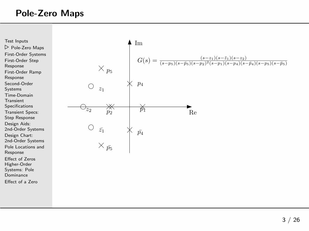
G(s) = (s−z1)(s−z1)(s−z2)(s−p5)(s−p5)(s−p2)2(s−p1)(s−p4)(s−p4)(s−p5)(s−p5)

First-Order Systems
Test Inputs
Pole-Zero Maps
⊲First-OrderSystems
First-Order StepResponse
First-Order RampResponse
Second-OrderSystems
Time-DomainTransientSpecifications
Transient Specs:Step Response
Design Aids:2nd-Order Systems
Design Chart:2nd-Order Systems
Pole Locations andResponse
Effect of ZerosHigher-OrderSystems: PoleDominance
Effect of a Zero
4 / 26
First-order systems are described by the I/O differential equation
τ c+ c = r(t)
or in TF formC(s)
R(s)=
1
τs+ 1
The number τ is called the time constant of the system. The TFhas one real pole at s = −
1τ.
Step Response
Applying the unit step input R(s) = 1
sgives the response
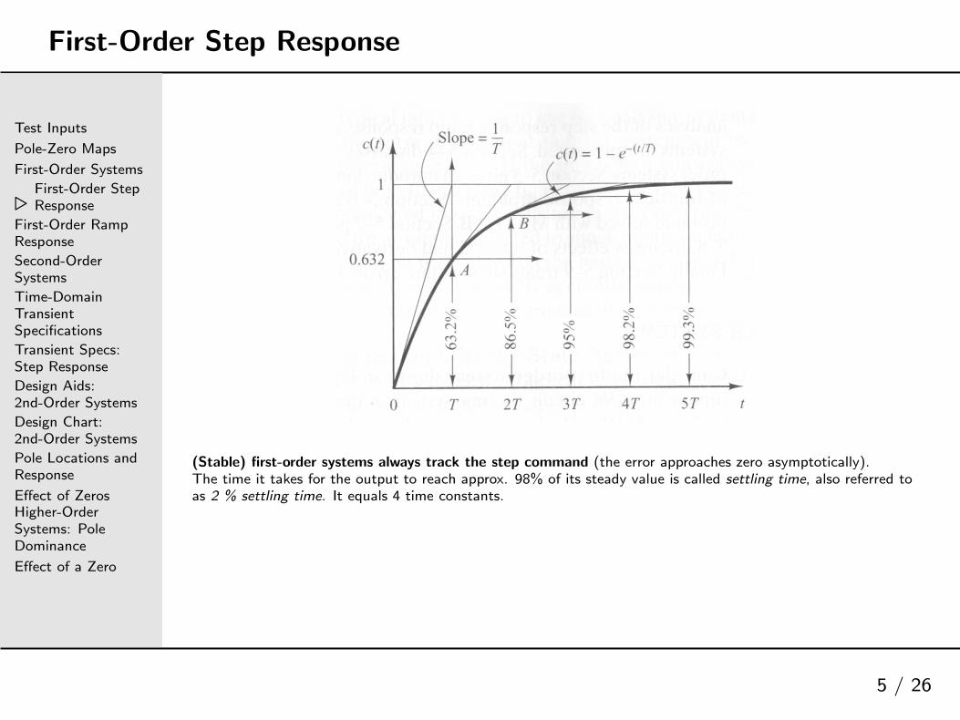
c(t) = 1− e−tτ
First-Order Step Response
Test Inputs
Pole-Zero Maps
First-Order Systems
⊲First-Order StepResponse
First-Order RampResponse
Second-OrderSystems
Time-DomainTransientSpecifications
Transient Specs:Step Response
Design Aids:2nd-Order Systems
Design Chart:2nd-Order Systems
Pole Locations andResponse
Effect of ZerosHigher-OrderSystems: PoleDominance
Effect of a Zero
5 / 26
(Stable) first-order systems always track the step command (the error approaches zero asymptotically).The time it takes for the output to reach approx. 98% of its steady value is called settling time, also referred toas 2 % settling time. It equals 4 time constants.

First-Order Ramp Response
Test Inputs
Pole-Zero Maps
First-Order Systems
First-Order StepResponse
⊲First-Order RampResponse
Second-OrderSystems
Time-DomainTransientSpecifications
Transient Specs:Step Response
Design Aids:2nd-Order Systems
Design Chart:2nd-Order Systems
Pole Locations andResponse
Effect of ZerosHigher-OrderSystems: PoleDominance
Effect of a Zero
6 / 26
First-order systems cannot track a ramp command. The tracking error is always equal to the time constant.

Second-Order Systems
Test Inputs
Pole-Zero Maps
First-Order Systems
First-Order StepResponse
First-Order RampResponse
⊲Second-OrderSystems
Time-DomainTransientSpecifications
Transient Specs:Step Response
Design Aids:2nd-Order Systems
Design Chart:2nd-Order Systems
Pole Locations andResponse
Effect of ZerosHigher-OrderSystems: PoleDominance
Effect of a Zero
7 / 26
The standard form of a second-order system is:
C(s)
R(s)=
w2n
s2 + 2ζwns+ w2n
where wn and ζ are called the natural frequency (in rad/s) anddamping ratio (dimensionless), respectively. The response willdepend on the nature of the poles:
� Underdamped: 0 < ζ < 1� Marginally Stable: ζ = 0� Critically Damped: ζ = 1� Overdamped: ζ > 1
Case 1: Underdamped (0 < ζ < 1)
Test Inputs
Pole-Zero Maps
First-Order Systems
First-Order StepResponse
First-Order RampResponse
⊲Second-OrderSystems
Time-DomainTransientSpecifications
Transient Specs:Step Response
Design Aids:2nd-Order Systems
Design Chart:2nd-Order Systems
Pole Locations andResponse
Effect of ZerosHigher-OrderSystems: PoleDominance
Effect of a Zero
8 / 26
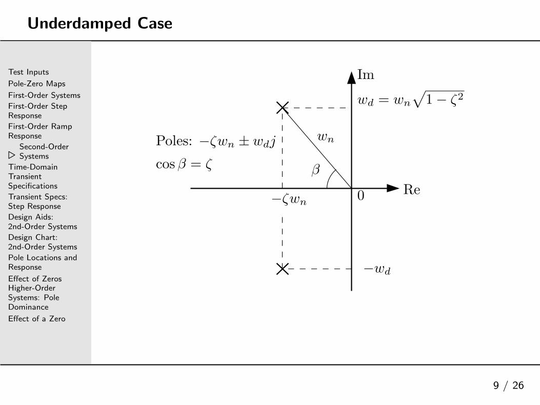
The poles are complex conjugates. The response to a unit step input isgiven by
c(t) = 1−e−ζwnt
√
1− ζ2sin
(
wdt+ tan−1
√
1− ζ2
ζ
)
where wd is the damped natural frequency:
wd = wn
√
1− ζ2
The damped natural frequency is the one obtained by counting thecycles per unit time in an experimental (and underdamped) responseand converting the result to radians per second.
Underdamped Case
Test Inputs
Pole-Zero Maps
First-Order Systems
First-Order StepResponse
First-Order RampResponse
⊲Second-OrderSystems
Time-DomainTransientSpecifications
Transient Specs:Step Response
Design Aids:2nd-Order Systems
Design Chart:2nd-Order Systems
Pole Locations andResponse
Effect of ZerosHigher-OrderSystems: PoleDominance
Effect of a Zero
9 / 26
wn
wd = wn
√
1 − ζ2
Re
Im
−ζwn
β
0
−wd
cos β = ζ
Poles: −ζwn ± wdj

Marginally Stable and Overdamped Cases
Test Inputs
Pole-Zero Maps
First-Order Systems
First-Order StepResponse
First-Order RampResponse
⊲Second-OrderSystems
Time-DomainTransientSpecifications
Transient Specs:Step Response
Design Aids:2nd-Order Systems
Design Chart:2nd-Order Systems
Pole Locations andResponse
Effect of ZerosHigher-OrderSystems: PoleDominance
Effect of a Zero
10 / 26
Marginally Stable Case (ζ = 0)When ζ = 0 the poles lie on the imaginary axis and the response to astep input is
c(t) = 1− coswnt
that is, the oscillation does not die out. The system oscillates with itsnatural frequency wn.
Critically Damped Case (ζ = 1)When ζ = 1 we get a real pole of multiplicity two at s = −wn. Theresponse is given by c(t) = 1− e−wnt(1 + wnt). No oscillations occurfor a step input.

Overdamped Case (ζ > 1)
Test Inputs
Pole-Zero Maps
First-Order Systems
First-Order StepResponse
First-Order RampResponse
⊲Second-OrderSystems
Time-DomainTransientSpecifications
Transient Specs:Step Response
Design Aids:2nd-Order Systems
Design Chart:2nd-Order Systems
Pole Locations andResponse
Effect of ZerosHigher-OrderSystems: PoleDominance
Effect of a Zero
11 / 26
When ζ > 1 the poles lie are real and unequal. The responsefeatures two decaying exponential terms (no oscillations):
c(t) = 1 +wn
2√
ζ2 − 1
(
e−s1t
s1−
e−s2t
s2
)
where the poles are
s1,2 = (ζ ±√
ζ2 − 1)wn

Normalized Second-Order Response
Test Inputs
Pole-Zero Maps
First-Order Systems
First-Order StepResponse
First-Order RampResponse
⊲Second-OrderSystems
Time-DomainTransientSpecifications
Transient Specs:Step Response
Design Aids:2nd-Order Systems
Design Chart:2nd-Order Systems
Pole Locations andResponse
Effect of ZerosHigher-OrderSystems: PoleDominance
Effect of a Zero
12 / 26

Time-Domain Transient Specifications
Test Inputs
Pole-Zero Maps
First-Order Systems
First-Order StepResponse
First-Order RampResponse
Second-OrderSystems
⊲
Time-DomainTransientSpecifications
Transient Specs:Step Response
Design Aids:2nd-Order Systems
Design Chart:2nd-Order Systems
Pole Locations andResponse
Effect of ZerosHigher-OrderSystems: PoleDominance
Effect of a Zero
13 / 26
� Many practical design cases call for time-domainspecifications
� Step response specs are often demanded (worst-case, drasticsituation)
� Common specifications
1. Rise time (Tr)2. Peak time (Tp)3. Percent overshoot (P.O.)4. Settling time (Ts)

Transient Specs: Step Response
Test Inputs
Pole-Zero Maps
First-Order Systems
First-Order StepResponse
First-Order RampResponse
Second-OrderSystems
Time-DomainTransientSpecifications
⊲Transient Specs:Step Response
Design Aids:2nd-Order Systems
Design Chart:2nd-Order Systems
Pole Locations andResponse
Effect of ZerosHigher-OrderSystems: PoleDominance
Effect of a Zero
14 / 26
0 Tr Tp Tset 2%0
Setpoint
FV
Second−Order Step Response Characteristics
Time (sec)
Setpoint
0.98*F.V
FinalValue
Overshoot
1.02*F.V
SteadyError

Design Aids: 2nd-Order Systems
Test Inputs
Pole-Zero Maps
First-Order Systems
First-Order StepResponse
First-Order RampResponse
Second-OrderSystems
Time-DomainTransientSpecifications
Transient Specs:Step Response
⊲
Design Aids:2nd-OrderSystems
Design Chart:2nd-Order Systems
Pole Locations andResponse
Effect of ZerosHigher-OrderSystems: PoleDominance
Effect of a Zero
15 / 26
� 2 % settling time: ts =4
ζwn
� Rise time: tr =π−βwd
� Peak time: tp =πwd
� Peak value: Mpt = (e−( ζ
√
1−ζ2)π
+ 1)y(∞)
� Percent overshoot: P.O.= 100e−( ζ
√
1−ζ2)π

Design Chart: 2nd-Order Systems
Test Inputs
Pole-Zero Maps
First-Order Systems
First-Order StepResponse
First-Order RampResponse
Second-OrderSystems
Time-DomainTransientSpecifications
Transient Specs:Step Response
Design Aids:2nd-Order Systems
⊲
Design Chart:2nd-OrderSystems
Pole Locations andResponse
Effect of ZerosHigher-OrderSystems: PoleDominance
Effect of a Zero
16 / 26

Pole Locations and Response
Test Inputs
Pole-Zero Maps
First-Order Systems
First-Order StepResponse
First-Order RampResponse
Second-OrderSystems
Time-DomainTransientSpecifications
Transient Specs:Step Response
Design Aids:2nd-Order Systems
Design Chart:2nd-Order Systems
⊲Pole Locationsand Response
Effect of ZerosHigher-OrderSystems: PoleDominance
Effect of a Zero
17 / 26

Effect of Zeros
Test Inputs
Pole-Zero Maps
First-Order Systems
First-Order StepResponse
First-Order RampResponse
Second-OrderSystems
Time-DomainTransientSpecifications
Transient Specs:Step Response
Design Aids:2nd-Order Systems
Design Chart:2nd-Order Systems
Pole Locations andResponse
⊲ Effect of ZerosHigher-OrderSystems: PoleDominance
Effect of a Zero
18 / 26
� The above design formulas are valid when no zeros arepresent.
� In general, zeros spoil the response by increasing theovershoot.
� If zeros are found on the r.h.p., the system is said to benonminimum phase, and the response is worsened.
� Zeros may be neglected in some cases (more about this laterin this lecture)

Higher-Order Systems: Pole Dominance
Test Inputs
Pole-Zero Maps
First-Order Systems
First-Order StepResponse
First-Order RampResponse
Second-OrderSystems
Time-DomainTransientSpecifications
Transient Specs:Step Response
Design Aids:2nd-Order Systems
Design Chart:2nd-Order Systems
Pole Locations andResponse
Effect of Zeros
⊲
Higher-OrderSystems: PoleDominance
Effect of a Zero
19 / 26
� When more than two poles are present, or when two distinctreal poles are present, it can be difficult to predict theresponse without computer simulation
� Frequently, one or two poles are dominant. Remember thateach single real pole gives rise to a term of the form a
s(s+a)when a step input is applied. If we invert the term, thecontribution of the pole is 1− e−at. So if the time constantof the pole (1/a) is very small, the transient is very short anddoes not contribute much to the overall response. On theother hand, poles with large time constants are the onesdictating the response. We say that such poles are dominant.The same applies to complex conjugate pairs, where the timeconstant taken into consideration is 1
ζwn.

Pole Dominance Criterion
Test Inputs
Pole-Zero Maps
First-Order Systems
First-Order StepResponse
First-Order RampResponse
Second-OrderSystems
Time-DomainTransientSpecifications
Transient Specs:Step Response
Design Aids:2nd-Order Systems
Design Chart:2nd-Order Systems
Pole Locations andResponse
Effect of Zeros
⊲
Higher-OrderSystems: PoleDominance
Effect of a Zero
20 / 26
� Begin by finding all poles of the TF and finding their timeconstants. Remember: For a real pole at s = −a, the timeconstant is 1/a, and for a complex conjugate pair with0 < ζ < 1, it is 1
ζwn.
� Sort out the time constants: (high) τ1, τ2..., τn (low).� Attempt to find a gap of a factor of eight or more between
two consecutive time constants, starting with the highest. Ifsuch a gap is found, neglect all poles on the fast side of thegap (small time constants).
� Careful! when reassembling the TF. You may beinadvertently changing the TF gain (a.k.a. DC gain): Makesure that the responses to a step input have the same finalvalue. If not, correct the reduced TF with an appropriateconstant.
Pole Dominance: Example
Test Inputs
Pole-Zero Maps
First-Order Systems
First-Order StepResponse
First-Order RampResponse
Second-OrderSystems
Time-DomainTransientSpecifications
Transient Specs:Step Response
Design Aids:2nd-Order Systems
Design Chart:2nd-Order Systems
Pole Locations andResponse
Effect of Zeros
⊲
Higher-OrderSystems: PoleDominance
Effect of a Zero
21 / 26
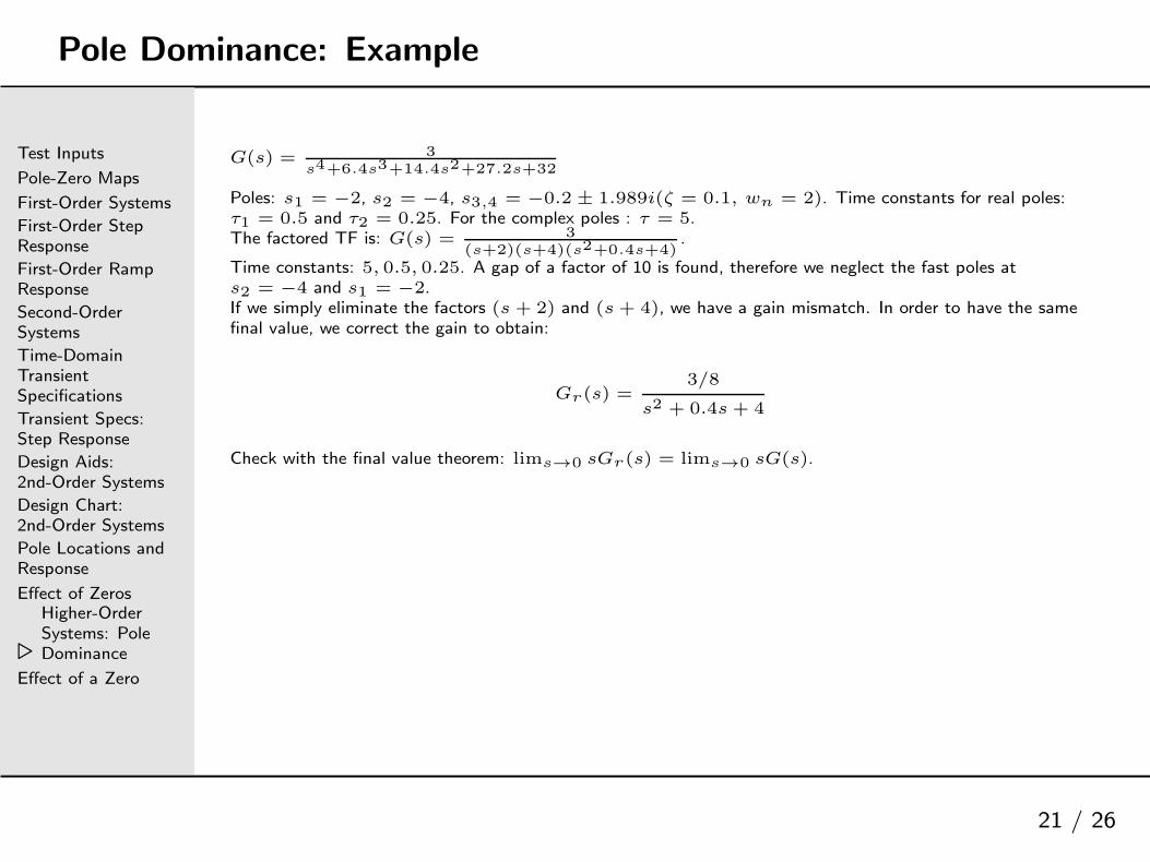
G(s) = 3s4+6.4s3+14.4s2+27.2s+32
Poles: s1 = −2, s2 = −4, s3,4 = −0.2 ± 1.989i(ζ = 0.1, wn = 2). Time constants for real poles:τ1 = 0.5 and τ2 = 0.25. For the complex poles : τ = 5.The factored TF is: G(s) = 3
(s+2)(s+4)(s2+0.4s+4).
Time constants: 5, 0.5, 0.25. A gap of a factor of 10 is found, therefore we neglect the fast poles ats2 = −4 and s1 = −2.If we simply eliminate the factors (s + 2) and (s + 4), we have a gain mismatch. In order to have the samefinal value, we correct the gain to obtain:
Gr(s) =3/8
s2 + 0.4s + 4
Check with the final value theorem: lims→0 sGr(s) = lims→0 sG(s).

Effect of a Zero
Test Inputs
Pole-Zero Maps
First-Order Systems
First-Order StepResponse
First-Order RampResponse
Second-OrderSystems
Time-DomainTransientSpecifications
Transient Specs:Step Response
Design Aids:2nd-Order Systems
Design Chart:2nd-Order Systems
Pole Locations andResponse
Effect of ZerosHigher-OrderSystems: PoleDominance
⊲ Effect of a Zero
22 / 26
For second-order systems, we can predict the effect of a single real zero on the overshoot. Consider
G(s) =(w2
n/a)(s + a)
s2 + 2ζwns + w2n
If a/ζwn > 8, neglect the zero due to dominance: Gr(s) =w2
ns2+2ζwns+w2
n. If not, use the chart:
Example
Test Inputs
Pole-Zero Maps
First-Order Systems
First-Order StepResponse
First-Order RampResponse
Second-OrderSystems
Time-DomainTransientSpecifications
Transient Specs:Step Response
Design Aids:2nd-Order Systems
Design Chart:2nd-Order Systems
Pole Locations andResponse
Effect of ZerosHigher-OrderSystems: PoleDominance
⊲ Effect of a Zero
23 / 26
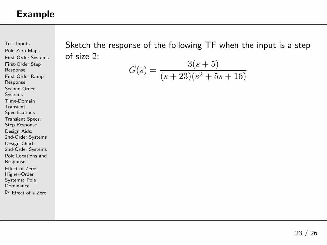
Sketch the response of the following TF when the input is a stepof size 2:
G(s) =3(s+ 5)
(s+ 23)(s2 + 5s+ 16)

Solution
Test Inputs
Pole-Zero Maps
First-Order Systems
First-Order StepResponse
First-Order RampResponse
Second-OrderSystems
Time-DomainTransientSpecifications
Transient Specs:Step Response
Design Aids:2nd-Order Systems
Design Chart:2nd-Order Systems
Pole Locations andResponse
Effect of ZerosHigher-OrderSystems: PoleDominance
⊲ Effect of a Zero
24 / 26

Solution
Test Inputs
Pole-Zero Maps
First-Order Systems
First-Order StepResponse
First-Order RampResponse
Second-OrderSystems
Time-DomainTransientSpecifications
Transient Specs:Step Response
Design Aids:2nd-Order Systems
Design Chart:2nd-Order Systems
Pole Locations andResponse
Effect of ZerosHigher-OrderSystems: PoleDominance
⊲ Effect of a Zero
25 / 26

Matlab Simulation
Test Inputs
Pole-Zero Maps
First-Order Systems
First-Order StepResponse
First-Order RampResponse
Second-OrderSystems
Time-DomainTransientSpecifications
Transient Specs:Step Response
Design Aids:2nd-Order Systems
Design Chart:2nd-Order Systems
Pole Locations andResponse
Effect of ZerosHigher-OrderSystems: PoleDominance
⊲ Effect of a Zero
26 / 26
0 0.5 1 1.5 2 2.5 3 3.5 4 4.5 50
0.01
0.02
0.03
0.04
0.05
0.06
0.07
0.08
0.09
0.1
c(t)
t
c(tp)=0.0919
ts=1.3 s
c(∞)=0.0815 Overshoot=12.76%
Top Related