


Languages
Pages
Legal


Childhood Immunization, Mortality and Human Capital
Accumulation: Micro-Evidence from India
Job Market Paper
Santosh Kumar ∗
November 2008
Abstract
In the mid-1980s, the Indian government embarked on one of the largest childhood immunization
programs-called “Universal Immunization Program” (UIP)-in order to reduce the high mortality and
morbidity among children. I examine the effect of this immunization program on child mortality and
educational attainment by exploiting district-by-cohort variation in exposure to the program. Results
indicate that exposure to the program reduced infant mortality by 0.4 percentage points and under-
five child mortality by 0.5 percentage points. These effects on mortality are sizable–they account
for approximately one-fifth of the decline in infant and under-five child mortality rates between
1985-1990. The effects are more pronounced in rural areas, for poor people, and for members of
historically disadvantaged groups. While the program clearly reduced mortality, it had mixed effects
on children’s educational outcomes. I find it had a negative impact on primary school completion,
but a positive impact on secondary school completion. The negative effect at low levels of schooling
may be due to lower average health among marginal surviving children or resource constraints faced
by the government where investments in child health programs may have crowded out investment in
school infrastructure and quality. The greater propensity to complete secondary school on the other
hand may be due to improved health among those farther away from the margin of survival.
JEL classification: I1, I2, J13, J18, O15.
Keywords: Immunization, Health, Schooling, India.
∗Ph.D Candidate, Department of Economics, University of Houston, Houston, TX, 77204 (e-mail: [email protected]). Pleasedo not cite without author’s prior permission. I thank Abhijit Banerjee, Aimee Chin, Chinhui Juhn, Rohini Pande and participantsat the XIIth Texas Econometric Camp, University of Houston Graduate Workshops and 8th Annual Missouri Economic Conferencefor helpful comments and discussions. Financial support from the University of Houston Department of Economics to collect datais gratefully acknowledged. Any error remains mine.
1 Introduction
Scientific evidence has shown that vaccines are effective in reducing childhood mor-
tality and morbidity (Levine et al., 2005; United Nations, 2006). Therefore, childhood
immunization has become a critical component of public health policies in many coun-
tries. Recent evidence suggests, however, that in many countries child mortality is either
increasing or stagnating despite these countries having an active childhood immunization
program in place (Adjuik et al., 2006; Aaby and Jenson, 2005). In addition, the level of
child mortality still remains unacceptably high in many parts of the world. For example,
the under-five mortality in 2003 was 9.2 percent in South Asia, 17.5 percent in Sub-
Saharan Africa, and only 0.06 percent in industrialized countries. (Glewwe and Miguel,
2008). In light of these numbers, the foremost question to ask is: are childhood immu-
nization programs effective in terms of reducing mortality, especially in poorer developing
countries? Answering this is of tremendous policy relevance considering the large number
of countries that have childhood immunization programs, or are considering adopting one.
In addition, we may care about the general question of long-run effects of child health
on educational outcomes. Although school enrollment and access to schools have grown
considerably in developing countries, 113 million primary-school-aged children were not
enrolled in 2001, most children never reach secondary school, and academic achievement as
measured by standardized tests is dismally low (Glewwe and Kremer, 2006). It is natural
to ask the extent to which poor child health is responsible for these poor educational
outcomes.
This paper takes a step toward addressing these questions by evaluating a large-scale
government-sponsored childhood immunization program in India called “Universal Immu-
nization Program” (hereafter, UIP). In 1985-86 the Government of India launched UIP
in 31 districts. Each year additional districts were phased into the program and by 1990
all 443 districts of India were covered by UIP. The program delivered free immunization
1
shots for children under one year of age to protect them from six Vaccine Preventable
Diseases (hereafter, VPDs).1
UIP has features that facilitate evaluation. On the one hand, there is district variation
in UIP exposure: UIP was implemented gradually across districts in India, with the timing
apparently determined by fixed district characteristics. On the other hand, there is cohort
variation in UIP exposure: only children who were twelve months old or younger at the
time the program began would have been eligible to receive free immunization shots.
This enables me to use a difference-in-differences-type estimation strategy to identify
the effect of UIP. The identifying assumption is that without UIP, the cohort difference
in mortality and educational outcomes would have been the same between the districts
that implemented UIP sooner and the districts that implemented UIP later. I apply
this identification strategy using the “Reproductive and Child Health Survey” (hereafter,
RCH), a large nationally representative individual-level data-set.
The main finding of this paper is that UIP reduced infant mortality by 0.4 percentage
points and under-five mortality by 0.5 percentage points. The effects on mortality out-
comes are substantial given that the infant mortality in India was 9.7% and under-five
mortality estimate was 15% before the launch of the program. Indeed they account for ap-
proximately one-fifth of the decline in infant and under-five child mortality rates between
1985-1990. There is no differential effect by gender but effects are more pronounced in
rural areas, for poor people, and low caste people. I verify that these results are not due
to differential trends in child mortality between early-UIP districts and later-UIP districts
by doing control experiments using older cohorts and using a health outcome unrelated
to the immunizations.
Next, I examine the effects of UIP on the educational outcomes of surviving children
and find mixed results. The program had a negative impact on primary school completion,
but a positive impact on secondary school completion. The results on education outcomes1The six VPDs are Diphtheria, Pertussis, Tetanus, Poliomyelitis, Measles and Tuberculosis.
2
can be explained in terms of change in the composition of the surviving children due to
the immunization program. The negative effect on education may be due to resource
constraints faced by the government. It may be possible that government’s financial and
physical resources were more devoted to public health programs, crowding out resources
for education. This may have had a hit on the school quality and infrastructure, causing
the students to drop out from primary school. Increased burden of siblings care can be
another factor responsible for the negative effect on education. On the other hand, the
result that UIP increased the education of some children is similar to the findings of Miguel
and Kremer (2004), Lucas (2005), Bobonis et al. (2006), Bleakley (2007) and Kremer et
al. (2007). The greater propensity to complete secondary school may be due to improved
health among those children who are not at the margin of survival.
This paper contributes to the existing literature in several ways. First, I am not aware
of any previous studies that rigorously quantify the effects of immunization programs on
children’s outcomes. On the one hand, there have been process evaluations which describe
the implementation of UIP and vaccination coverage. On the other hand, there have been
medical evaluations which examine the effects of immunizations on health outcomes but
these studies are conducted in laboratory-like settings rather than in actual developing-
country contexts. There is widespread skepticism about the public health service delivery
system in developing countries. Chaudhury et al. (2006) find, for instance, that 39%
of doctors and 31% of other health care workers were absent from work in nationally
representative surveys of primary health centers in Bangladesh, Ecuador, India, Indonesia,
Peru and Uganda. In these environments, can a mass immunization program successfully
reduce child mortality? What are the consequences for children’s educational outcomes?
Second, this paper adds to the literature on the effects of child health on schooling.
Most studies linking health and education are unable to distinguish causality from mere
correlation, though there are a few recent exceptions (including Miguel and Kremer, 2004;
Lucas, 2005; Bobonis et al., 2006; Bleakley, 2007; Kremer et al., 2007; see Glewwe and
3
Miguel, 2008 for a review). None of the studies estimating the causal effect of health
on education have used variation in health provided by an immunization program. Im-
munization programs provide a new and different source of variation in child health. In
particular, whereas health interventions used by other studies primarily reduce the mor-
bidity of children, immunization programs reduce both the mortality and morbidity of
children. Since immunization programs operate on different margins, the consequences
for education could be different from those other health interventions.
The rest of the paper is structured as follows: in Section 2, I discuss the related
literature and provide an overview of UIP. Section 3 presents the empirical framework
and Section 4 describes the data. Section 5 presents the results on mortality outcomes
and Section 6 presents the results on educational outcomes. Finally, Section 7 concludes.
2 Background
2.1 The Universal Immunization Program
Approximately 3 million children die each year of VPDs with a disproportionate number
of these children residing in developing countries (Kane and Lasher, 2002). Vaccines
remain one of the most cost-effective public health initiatives, yet the cover against VPDs
remains far from complete; recent estimates suggest that approximately 34 million children
are not completely immunized with almost 98 percent of them residing in developing
countries (Frenkel and Nielsen, 2003). Reducing child mortality by two-thirds between
1990 and 2015 is the fourth of eight Millennium Development Goals endorsed by world
leaders in the Millennium Declaration in 2000.
In India, immunization of children against VPDs has been a central goal of the health
care system from the 1970s. The Expanded Program on Immunization (hereafter, EPI)
was initiated in 1978 to make six childhood vaccines (BCG, DPT, TT, DT, Polio and
Typhoid) available to all eligible children. The main objective of EPI was to reduce mor-
4
tality and morbidity by controlling six target diseases- Tuberculosis, Diphtheria, Tetanus,
Pertussis, Polio and Typhoid. EPI failed to achieve the objective of immunizing children;
because the program was limited primarily to major hospitals in urban areas and cover-
age levels were very low. Failure of EPI led the Government of India to make childhood
immunization a top priority. In 1985, the Government of India made childhood immu-
nization a Technology Mission and launched UIP with much dynamism to attain the goal
of achieving 85 percent coverage for Tuberculosis, Diphtheria, Tetanus, Pertussis, Polio
and Measles for all children by 1990.
Under UIP, each child had to be vaccinated before he or she turned one year of age
with three doses of DPT vaccine, three doses of polio vaccine and one dose each of measles
and BCG vaccine. Table 1 in the appendix lists some symptoms associated with the
diseases that these shots protect against. The symptoms range from mild to severe, with
serious sickness and death more likely among infants (whose immune systems are not yet
mature) and poor children (whose immune systems are weakened due to malnutrition). It
is worth noting that immunization protects individuals not only from illness per se, but
also from the long-term effects of that illness on their physical, emotional, and cognitive
development (Bloom et al., 2005). Additionally these diseases are communicable, so there
are significant positive externalities from being vaccinated. That is, the vaccines reduce
the risk of disease not only for the children vaccinated but also for people around them
by reducing the transmission rate of the diseases.
There were not sufficient resources to implement the program all over the country at
the same time. Thus, UIP had a phased roll-out, beginning with 31 districts in 1985-86
and covering all districts by 1990. The program was implemented through the existing
network of primary health care infrastructure which consists of a referral center called
“community health center” for every 80 to 120 thousand people, a primary health center
for 20 to 30 thousand people, and a sub-center for every 3 to 5 thousand people. The
program made provision for additional inputs in the form of additional staff, vaccines, and
5
equipment for storage and transportation of vaccines such as walk-in-coolers, refrigerators
and vaccine carriers.
Below I take advantage of the staggered implementation of UIP across districts to help
identify UIP’s effect, therefore it is essential to understand what determined the timing.
Toward this end, I had numerous conversations with officials in the UIP division of the
Ministry of Health and Family Welfare. The timing was not completely random. It seems
that the capacity of the district to achieve the immunization coverage rates targeted by
UIP and to maintain this level in subsequent years was a major factor in the selection
of the district. In addition, infrastructure and other health facilities to deliver the UIP
services were also taken into account while selecting the districts. In other words, selection
of districts was based on fixed characteristics of the districts. For example, early-adopting
districts may have more primary health centers, more nurses, or have better health care
infrastructure. Selection on fixed district characteristics does not cause problems for
the interpretation of my estimated treatment effects because they rely on within-district
variation in exposure to UIP only; that is, I always control for district fixed effects. A
more serious problem would be if the timing of implementation depended on underlying
district-specific trends in the outcome variables. It must be emphasized that UIP officials
never indicated that district trends in mortality or education were part of the criteria
for earlier implementation. However, to address this potential concern, I perform control
experiments using older cohorts who are not exposed to UIP and using a health outcome
unrelated to the immunizations; I discuss these control experiment in detail in section 5.
UIP is one of the largest in the world in terms of quantities of vaccines used, number
of intended beneficiaries, number of immunization sessions organized, the geographical
spread and the diversity of areas covered. Surprisingly, there have not been any studies
estimating UIP’s effect on mortality, much less education. Previous evaluations of UIP
were mostly sanctioned by Ministry of Health and Family Welfare and international donor
agencies like WHO, UNICEF and were basically process evaluations that look at the cov-
6
erage of vaccines.2 They show that UIP was able to substantially increase the coverage of
immunization shots (Figure 1 in Appendix ). Vaccine coverage by antigen shows substan-
tial increase during the UIP period. The vaccine coverage increased from a low 30-40%
at the start of the program to approximately 80-100% by 1990-91.
The extent to which UIP reduced child mortality and its effects on the schooling of
surviving children remains an open questions. Answering these questions is of great in-
terest for India. There is widespread debate about the proper implementation of public
health programs in India. Many claim that the public health service delivery system in
India is inefficient and that government-sponsored programs exist only on paper and real
take-off of public health programs is either doubtful or slow. Moreover, it should have rel-
evance for policymakers and public health activists outside of India. Many countries have
mass immunization programs or are considering adopting them. Immunization programs
compete for limited funding for public health initiatives and other welfare programs, with
budget constraints especially tight in poor developing countries. Do immunization pro-
grams help the intended beneficiaries? I present my strategy for evaluating UIP after
briefly reviewing the related literature.
2.2 Related Literature
I am not aware of any studies that rigorously quantify the effect of a childhood immu-
nization program on mortality and educational outcomes in a developing country setting.
However, this paper is related to two literatures which I discuss briefly below. First is
the medical literature on the impact of immunization vaccines on mortality and other
health outcomes. Second is the economics literature on the causal effect of child health
on educational outcomes.
In the medical literature, there have been several types of studies. First are clinical
trials of vaccines. These trials have firmly established that the DPT vaccine effectively2Gupta and Murali (1989); Sathyamala (1989); Annual Report (1987-88), MoHFW; UNICEF Coverage Survey 2002; WHO
Review (2004).
7
protects against diphtheria, pertussis and tetanus; the BCG vaccine against typhoid and
the measles and polio vaccines against measles and polio, respectively (Levine et al.,
2005; United Nations, 2006). There have also been a few epidemiological studies in
developing countries which examine the impact of specific vaccines on child mortality
(Breiman et al., 2004 for Matlab, Bangaladesh; Koeing et al., 1990 for Senegal). These
studies reconfirms the laboratory evidence and find decreased risk of death for vaccinated
children. The sample sizes tend to be small in these studies, unfortunately. Finally,
there are numerous studies that examine the cost-effectiveness and cost-benefit of vaccines
(Navas, 2005; Ekwueme, 2000; see Bloom, Canning and Weston, 2005 for a review). These
studies look at outcomes like averted illnesses, hospitalizations and deaths, disability-
adjusted life years (DALYs) gains, and medical costs. These studies suggest immunization
is a highly cost-effective intervention. This medical research underlies the public health
policy of many countries to require vaccinations for all children.
This paper differs from the medical studies in several respects. First, it is evaluating
the effect of a program that provided vaccinations, not the effect of the vaccinations
as the medical studies have done. Although we know scientifically that vaccinations
reduce mortality, we do not know whether a mass childhood immunization program can
be effective in reducing mortality in a poor developing country such as India. The success
of the program depends not only on the efficacy of the vaccinations but also the public
health delivery system. Second, given the low baseline vaccination coverage and average
health status in poor developing countries, it may well be that the marginal impact of the
vaccinations may be greater than in developed countries where the medical studies were
done. Third, the medical literature has ignored non-health outcomes such as education.
There is a large body of literature in economics that shows positive correlations between
health and education. Glewwe and Miguel (2008) provide a review. It is difficult to infer
the causal effect of health on education from these studies since it is easy to imagine that
it may be education that is affecting health, or some omitted variable that is affecting
8
both health and education. Behrman (1996) argues that existing evidence on child health
and education (at least up to the time of his paper) is inconclusive because of the difficulty
in separating causality from correlations.
More recently, researchers have used randomized experiments and natural experiments
to identify the causal effect of health on education. In randomized experiments, the re-
searcher randomly assigns similar units to different health treatments (a treatment group
that receives a medical treatment and a control group that doesn’t), generating an ex-
ogenous source of variation in health. Randomized experiments examining the effect of
child health on education include the following. Miguel and Kremer (2004) find that pro-
viding children with deworming medication significantly reduced serious worm infections
and increased school attendance. Bobonis, Miguel and Sharma (2006) find that a iron
supplementation program significantly reduced anemia and school absenteeism. Vermeer-
sch and Kremer (2004) find that a school breakfast program significantly raised preschool
attendance and cognitive test scores.
Researchers have also used natural experiments to identify the effect of child health on
educational outcomes. Along these lines, Bleakley (2007) exploits region-by-time variation
in exposure to the hookworm eradication program sponsored by the Rockefeller Sanitary
Commission in the 1910s in the United States to identify the effects of reducing hook-
worm infections on educational outcomes. He finds that regions that experienced greater
reductions in hookworm infections had larger increases in school attendance and literacy.
Few working papers also use a difference-in-differences strategy to estimate the effect of
malaria on human capital accumulation (Bleakley, 2007 for the U.S., Brazil, Colombia and
Mexico; Kremer et al., 2007 for India; Lucas, 2005 for Sri Lanka, Paraguay and Trinidad).
This paper takes the tactic in this latter group of studies by taking advantage of a
natural experiment to identify the effect of health on education. As described in the next
section, I use district-by-cohort variation in exposure to UIP to obtain estimates of the
effect of health on education. It is one of only a handful of studies that addresses the issue
9
of endogeneity in health when estimating the effect of health on education. Moreover, it
uses a new and different source of variation in child health than has never been used before.
In particular, none of the previous studies have looked at the impact of an immunization
program. Immunization programs affect both mortality (of the youngest children) and
morbidity (of older individuals). In contrast, the aforementioned studies that estimate
the causal effect of health on education use health interventions-deworming treatments,
malaria treatments and school meals for school-aged children-that operate primarily on
the morbidity margin.
3 Empirical Framework
The objective of this study is to estimate causal impact of a developing-country im-
munization program on child mortality and education outcomes. Ideally to identify the
effect, we would conduct a randomized experiment where some children are placed into
a treatment group that receives immunizations and others are placed in a control group.
We would follow these children over time and compare their mortality and educational
outcomes. The control group describes the counterfactual of what the treatment group’s
outcomes would have been had the medical intervention not occurred. This is a simple
and convincing approach since at the outset of the experiment, the children were similar.
In the absence of a randomized experiment, I rely on a natural experiment. I use
variation provided by India’s implementation of UIP in the 1980s. In particular, I estimate
the program effect by utilizing the following two sources of variation in exposure to UIP:
variation across districts and variation across cohorts. First, variation across districts
comes from the fact that districts got the program in different years. Figure 2 in the
appendix shows the number of districts added on to UIP each year. UIP was implemented
in 48 districts (31 according to old district definitions) in the first year, 92 additional ones
in the second year and so on until all 563 districts (443 according to old district definitions)
10
were covered in 1990.3 Second, variation across cohorts comes from the fact that only
children who are twelve months or younger when UIP was implemented would have been
eligible to receive the shots. Table 2 in the appendix shows the schedule for the vaccines
that UIP provided; the shots are administered on a strict schedule in the first year of a
child’s life for maximal efficacy. Children older than one year were not treated by UIP.
Table 3 of the Appendix shows the birth cohorts that were eligible for UIP by district’s
year of UIP inception. For example, a child born in 1985 would have been exposed to
UIP if he lived in one of the 48 districts that implemented UIP first (in 1986), but not if
he lived in a district that implemented UIP later.
The difference-in-differences approach uses only the within-district cross-cohort varia-
tion in exposure to UIP to identify the effect of UIP. This is elaborated next.
3.1 Difference-in-Differences Strategy
Consider the following equation:
Yicd = β0 + β1UIPicd + δXicd + eicd (1)
where Yicd is the outcome variables for an individual i, in cohort c, residing in district
d. UIPicd indicates exposure to UIP and X is a vector of individual and household
characteristics (e.g., sex, caste, religion, age, birth order, mother’s education, mother’s
age, rural/urban). eicd is the error term.
We wish to estimate the effect of UIP so the parameter of interest in this equation is
β1. But β1 in equation (1) may not be consistently estimated due to omitted variable
bias. Districts may be different from each other on many unobserved dimensions that
can affect the outcome variables. For example, UIP officials indicated that the timing of
UIP implementation across districts was not random and instead apparently determined3The number of districts increased from 443 to 593 between the UIP period (1985-1990) and the RCH survey year (2002-04).
The data section has more details.
11
by some features of districts that could be considered constant over time such as health
infrastructure. Similarly, each cohort can also be systematically different in ways that
affect the outcome variables. For example, there is progress in health and education over
time, or some country-wide economic shocks in a particular year may affect that year’s
cohort differently than the another year’s cohort. I address these concerns by adding
district fixed effects and cohort fixed effects to equation (1):
Yicd = β0 + β1UIPicd + γd + φc + δXicd + eicd (2)
where Yicd is the outcome variables for an individual i, in cohort c residing in district d.
UIPicd indicates exposure to UIP. γ and φ are district and cohort fixed effects, respectively.
X is individual and household controls.
The parameter β1 in equation (2) can be interpreted as the causal effect of UIP under
the assumption that the difference in outcomes between the younger and older cohorts
would have been the same between earlier-implementing districts and later-implementing
districts in the absence of UIP. 4 In other words, the parallel trend assumption should be
satisfied. While it is not possible to directly test this assumption-it is a counterfactual-I
can assess its validity in a couple of ways. Below, I do this by: (1) estimating equation
(2) using only older cohorts that have never been exposed to UIP but where I falsify their
treatment status; and (2) estimating equation (2) using an outcome that is unlikely to be
affected by the program.
The identifying assumption would also be violated if there were some other contem-
poraneous interventions that had the exact same district-by-cohort variation as UIP and
which also affect the outcome variables I examine. To the best of my knowledge, I am not
aware of any child health or education intervention that can contaminate the identification
of the effect of the UIP.4If UIP exposure were a simple interaction between two binary variables, say being in an earlier-implementing district and
being in a younger birth cohort, then β1 would be a differences-in-differences estimate, i.e., the cohort difference in outcome inearlier-implementing states that is in excess of the cohort difference in later-implementing states. In fact I use more variation in UIPexposure but the intuition is similar to the simple binary case and so I term my approach a difference-in-differences-type strategy.
12
The parameter β1 in equation (2) may underestimate the true effect of UIP for a couple
of reasons. First, because consumption of vaccines has a positive externality, it is possible
that the control group benefits indirectly from UIP. That is, although the control group
is not eligible for UIP vaccinations, they may benefit because the diseases spread more
slowly when more people are vaccinated. Second, recall that the EPI program preceded
the UIP program in India. The EPI had very low vaccination coverage rates and operated
only out of major hospitals so it is unlikely to pose a significant problem. But it is
quite likely that the control (i.e., older) cohorts in urban areas got vaccinated under
EPI, which means the treatment group is partially treated already. This would cause me
to underestimate the program effect in urban areas. Third, inter-district movement of
households across districts may confound the estimated effects, but it is not much of a
concern here, because of limited inter-district migration in India (Munshi and Rosenzweig,
2006; Chatttopadhyay and Duflo, 2004).
3.2 Allowing for Heterogeneity in Program Effects
UIP may not have uniform impacts. The impact may differ based on child sex, so-
cioeconomic status, rural/urban, caste, etc. For example, perhaps the rich would have
immunized their children even in the absence of the program and it is the poor who would
benefit more from the program. On the other hand, there are also stories of “elite capture”
and it is possible that rich and elite class capture most of the benefits of the program. As
another example, the program may have different impacts in rural areas from urban areas
due to differences in the availability of health care infrastructure to deliver the services.
Also, the program effect may vary by gender. Oster (2007) shows that girls in India are
discriminated against in access to vaccination.
To test whether the program effect varies by sex, I estimate the following equation:
Yicd = β0 + β1UIPicd + β2UIPicd ∗ Femaleicd + β3Femaleicd + γd + φc + δXicd + eicd (3)
13
where the omitted category is male. β1 measures the average program effect for male
children and β2 captures the additional program effect for females.
Similarly, to examine whether there is a differential program impact by rural residence,
I estimate the following equation:
Yicd = β0 + β1UIPicd + β2UIPicd ∗Ruralicd + β3Ruralicd + γd + φc + δXicd + eicd (4)
where the omitted category is urban residence. β1 captures the program effect for children
residing in urban areas and β2 captures the additional program effect of residing in rural
areas.
Next, I allow the program effect to vary by socio-economic status of the household.5
To capture the heterogeneity in treatment effect by household socio-economic status, I
estimate the following equation:
Yicd = β0 + β1UIPicd + β2UIPicd ∗ Lowicd + β3UIPicd ∗Middleicd
+β4Lowicd + β5Middleicd + γd + φc + δXicd + eicd
(5)
where the omitted category is households with high socio-economic status. β1 captures
the program effect for children residing in household with high socio-economic status, β2
captures the differential program effect for children residing in household with low socio-
economic status (relative to the high category) and β3 captures the differential program
effect for children residing in household with middle socio-economic status.
To estimate how the program effects differ by social group, I estimate the following5The survey asks whether the household owns the following consumer durables: radio, television set, refrigerator, bicycle,
motorcycle and car. Based on ownership of these consumer durables, the RCH survey categorizes the household into three differentcategories in terms of socio-economic status: Low, Middle, and High. Though this is not the perfect measure of household wealthstatus, this is the best we can do given the fact that the health survey does not collect direct information on the income and wealthof the households.
14
equation:
Yicd = β0 + β1UIPicd + β2UIPicd ∗ SCicd + β3UIPicd ∗ STicd + β4UIPicd ∗OBCicd
+ β4SCicd + β5STicd + +β6OBCicd + γd + φc + δXicd + eicd
(6)
where the omitted category is household from high caste groups. β1 captures the program
effect for children belonging to high caste groups, β2 captures the differential program
effect for children belonging to Schedule Castes (SC) (relative to the high castes), β3
captures the differential program effect for children belonging to Schedule Tribes (ST)
and β4 captures the differential program effect for children belonging to Other Backward
Castes (OBC). SCs and STs are historically disadvantaged minority groups in India.
OBCs are not as poorly off as SCs, but also have faced discrimination historically.
4 Data
My empirical analysis uses data from two sources: individual-level data from the Re-
productive and Child Health (RCH) Survey and administrative data about UIP from the
Ministry of Health and Family Welfare, Government of India.
The RCH survey is a large, nationally representative survey. RCH survey is a District
Level Household Survey (DLHS) which has two waves. The first wave was conducted
in 1998-99 in 504 districts and second wave was conducted in 2002-04 in 593 districts.
Due to the timing of UIP, it is appropriate to use the second wave of the RCH survey.
The survey contains information about 6,20,107 households and 3.2 million individuals.
From these households, 5,07,622 eligible women, currently married aged 15-44 years whose
marriage was consummated were interviewed. The survey is designed to collect data on
marriage, fertility, family planning, reproductive health, maternal and child health, and
HIV/AIDS. First, I use the “fertility file” to construct the sample for my child mortality
analysis. Fertility history is collected for one woman who is aged 15 to 44 from each
15
surveyed household. Women are asked about their birth history, including children ever
born, dates of birth, if the children are alive, and, if not, when they died.6 This enables
me to collect for each child born to a woman in the fertility file the year of birth, whether
he/she has died and if so, when he/she died. Second, I use the“household file”to construct
the sample for analyzing the educational outcomes of surviving children. Both the fertility
and household files contain information on such control variables as district, rural/urban,
child sex, age, and birth order, and household social group, religion and socio-economic
condition.
The Ministry of Health and Family Welfare provided administrative information about
UIP. First, I talked to several UIP officials to find out the details of how UIP was imple-
mented. It was these conversations that led me to believe that the timing of UIP could be
considered conditional on district fixed effects, leading me to the difference-in-differences
strategy. Second, I obtained from them a list of new districts that implemented UIP each
year, from year 1 (1985-86) to year 5 when all districts were covered (1989-90).
I mapped the year of UIP implementation from the district-level administrative data
back to the individual-level RCH survey data using the district codes. One complication
was that the number of districts increased from 443 to 593 between the UIP period (1985-
1990) and the survey period (2002-04). Either an existing district split into two or more
new districts or a new district was formed by taking areas from two or more districts. I
successfully match 563 districts by looking at district census handbooks, district websites
and other government sources (a success rate of 95 percent).
The main outcome variables for my mortality analysis are the probability of dying
within the first twelve months (which I label Pr(Infant Mortality) and the probability of
dying within the first five years (Pr(Under-five Mortality)). Both infant mortality and
under-five mortality are common health indicators used by governments and international6One may question the reliability of these information as they are subject to severe recall bias especially in the case of older
children or girls. I checked the reliability of mortality information used in my analysis. The infant mortality in my sample is 9%as displayed in Table 1 and the official estimate given by SRS for the same period is 9.7%, which is quite close. Similarly, mysample estimate of under-five mortality of 11% also comes very close to official estimate of 12.3%, as given by SRS. SRS is SampleRegistration System that gives the official estimate of vital statistics in India.
16

agencies. Under-five mortality is an indicator of the cumulative exposure to mortality
risk during the most vulnerable years of childhood; it includes infant mortality as well as
mortality from age 1 to 5.
For my analysis of the educational outcomes of surviving children, the main outcome
variables are Pr(Literate), Pr(Primary School Completion), Pr(Middle School Comple-
tion), Pr(Secondary School Completion) and Years of Schooling. All the education out-
comes variables are dichotomous variables except Years of Schooling and are defined as fol-
lows. Pr(Primary School Completion) is defined as Pr(Years of Schooling ≥5), Pr(Middle
School Completion) is defined as Pr(Years of Schooling ≥8), Pr(Secondary School Com-
pletion) is defined as Pr(Years of Schooling ≥10). The education outcomes variables are
conditional on being literate.7
Table 1 shows the descriptive statistics of the variables used in the mortality and
education analyses. The paper uses children born between 1983 and 1992 for the mortality
outcomes and children born between 1983 to 1997 for the educational outcomes. The
number of observations for child mortality analysis is 297,385 and for education analysis
there are 898,789 observations.8 In the child mortality sample, 69 percent of the children
lives in rural areas and 47 percent belongs to a poor household. Majority of the children
are Hindu (76 percent) and disadvantaged minority group ST and SC forms 33 percent
of the sample. The mean mother’s age is 37.1 years and only 39 percent of the mothers
are literate. The mean mother’s age is higher than the mother’s age of the average child
because the survey was done in 2002-04 and the paper uses the children born between
1983 and 1992. The demographic and family characteristics of sample used in education
analysis are similar to the sample used in child mortality analysis.
In the child mortality sample, the mean infant mortality rate is 9% and the mean under-
five mortality rate is 11%. In the education sample, 82 percent of the children are literate7The survey asks Years of Schooling question only to the literate individuals.8Different samples are used for the child mortality analysis and education analysis because as explained earlier in this section,
the data for the mortality analysis are from the “fertility file” of the RCH and the data for the education analysis are from the”household file”. Only one woman aged 15-44 from each household answers the supplemental fertility questions, hence the smallersample size.
17
and conditional on being literate the average years of schooling is 6.2 years. Conditional
on being literate, about 65 percent children have completed primary schooling, 36 percent
have completed middle school and only 18 percent of children have completed secondary
school. The mean age of the children is 13.71 years; some of the children in the sample
are still in school.
5 Effect of UIP on Child Mortality
5.1 Basic Results
Table 2 reports the results of estimating equation (1) and equation (2) for infant mor-
tality and for under-five mortality.9 The main coefficient of interest is the coefficient for
the variable “Exposed to UIP”, which gives the average program effect. Column (1) and
Column (3) show the naive estimates of the program effect by estimating equation (1).
Estimates from Column (1) and Column (3) suggest a significant negative impact of the
program on Pr(Infant Mortality) and Pr(Under-Five Mortality). Results from column (1)
and Column (3) suggest that the program decreases the probability of infant mortality by
2.2 percentage points and the probability of under-five mortality by 2.8 percentage points.
On comparing the naive estimates with difference-in-differences estimates in Column (2)
and Column (4), it turns out that naive estimates grossly overestimate the program effect.
Estimating equation (1) is not the correct approach because districts differ in their fixed
characteristics and ignoring these fixed differences would bias the program effect. In par-
ticular, UIP officials stated that the timing of UIP was not random, and instead districts
that had better health care infrastructure received it sooner. Given this statement, it is
not surprising that the estimates in columns (1) and (3) are so large-they encapsulate not
only the true effect of UIP but also the effect of being in a district with better health care
infrastructure (which not surprisingly has a large negative effect on mortality!). Simi-
9I estimate these models using OLS, i.e., using the linear probability model with standard errors clustered at the district level.I also estimated these models using logit and find qualitatively similar results; these results are available upon request.
18
larly, there could be cohort-specific characteristics and without taking in account of these
characteristics, it is not possible to get the true effect of the program. For example,
there is improvement in health conditions and care in India over time, so younger cohorts
would have lower mortality even without UIP and the estimates in columns (1) and (3)
erroneously attribute these secular improvements over time to UIP.
The naive estimates in columns (1) and (3) highlight the dangers of giving causal
interpretations to parameter estimates when the sources of variation are not plausibly
exogenous, and motivate my difference-in-differences approach. The preferred estimates
are in Columns (2) and (4)-these are results from estimating equation (2), which includes
district fixed effects and year of birth fixed effects. Results from Column (2) and Column
(4) suggest that the program significantly reduces infant mortality and under-five mor-
tality. UIP decreases the probability of infant mortality by 0.4 percentage points, and
the estimate is statistically significant at 10 percent level of significance (column 2). The
official estimate of infant mortality was 9.7 percentage points in 1985 and 8 percentage
points in 1990. The 0.4 percentage point effect of UIP is 4.1% of the baseline infant mor-
tality rate and a fifth of the decline in infant mortality between 1985-1990. Thus, over a
short period, UIP caused a meaningfully sized reduction in infant mortality; it took India
thirty-four years to bring down the infant mortality from 14.6% in 1951 to 9.7% in 1985.
Column(4) reports the results for under-five mortality. Results show that the program
has a negative and significant impact on under-five mortality. The program reduced under-
five mortality by 0.5 percentage points. The under-five mortality was 15 percentage points
in 1985 and reduced to 12.3 percentage points by 1990. The 0.5 percentage point effect of
UIP is 3.3% of the baseline under-five mortality rate and almost a fifth of the decline in
under-five mortality between 1985-1990. It should be noted that the program has a larger
impact on under-five mortality compared to infant mortality. This is to be expected
because the under-five mortality rate includes infant mortality as well as mortality of
children aged 1 up to 5. Thus there is a tenth of a percentage point decline in the
19
mortality of children aged 1 up to 5 (fourth tenths of a percentage point is the decline in
mortality of children up to age 1). It makes sense that the mortality declines are greatest
for infants. Vaccinations under UIP begin at birth, and though maximal protection is not
gained until all the doses are administered according to schedule, protection begins right
away. This early protection makes a big difference for infant survival since infants do not
have well developed immune systems yet.
In all the regression models in Table 2, the signs of the control variables are as expected.
Mother’s age and mother’s education have negative and significant effect on infant and
under-five mortality. Poor and disadvantaged minority children(ST and SC) are more
likely to die. For Other Backward Caste and Hindu children, the estimates are positive and
significant, meaning that children belonging to these categories have higher probability of
dying.
5.2 Heterogeneity in Program Effects
Table 3 and Table 4 show the results from estimating equations (3)-(6) where the effect
of the program on mortality outcomes vary by gender (column 1), by rural (column 2),
by caste (column 3) and by socio-economic status (column 4). Table 3 reports the results
on infant mortality and Table 4 reports the results on under-five mortality. Column (1)
of Table 3 suggests that UIP did not have a different effect for boys and girls, i.e., infant
mortality decreased by about the same amount for both girls and boys due to UIP (though
the point estimate is negative for girls, suggesting that girls might have benefited a little
more). Column (2) suggests that the program had a zero effect in urban areas (the point
estimate is 0.05 percentage points and is insignificant) and rural areas had a negative
effect that is significantly different both from the urban effect and from zero at 5 percent
level of significance. That a reduction in child mortality is found only in rural areas may
be due to urban people already having access to vaccinations even before UIP or just that
health conditions and care tend to be better in urban areas (as indicated by the much
20
lower infant mortality rates at the outset). Thus there is more room for improvement in
the rural areas, and that is where I find mortality effects. In Column (3), the program
effects are negative for SC and OBC children; these effects are both significantly different
from zero and from the effect for higher caste groups. The effect for ST children is negative
but not significant.10 Finally, the program also has negative and significant impact on
infant mortality for children from poor households (column 4). There was no reduction in
mortality among children from middle- and high-income households. Columns (3) and (4)
both inform on whether the effects of UIP vary by household socioeconomic status (there
is much overlap between being in a low social group and being poor), and they both clearly
show that it is the children from disadvantaged households who experience the declines
in mortality; there is no effect of UIP on higher caste groups or the middle-income and
rich. Children from higher caste and non-poor households have lower mortality rates at
the outset, and may have been getting vaccinated to some extent already.
I show the results for under-five mortality in Table 4. They are similar to the infant
mortality results in Table 3 except the estimated reduction in mortality is higher for
reasons stated earlier (the under-five mortality measure includes mortality of infants and
older children). As before, it appears to be the children from rural, lower caste groups
and poor households who are benefiting from UIP in terms of increased survival rate.
5.3 Testing for Differential Trends in Child Mortality
The identifying assumption for my empirical strategy is that in absence of the program,
the difference in outcomes of younger and older cohorts would be the same between earlier-
implementing districts and later-implementing districts. We would not be able to interpret
the coefficients for “Exposed to UIP” in Table 2-4 as the causal effect of the immunization
program if the aforementioned were not true. In this subsection, I assess the validity of10Similar to the SC and the OBC, the ST are also a disadvantaged group with higher-than-average child mortality so perhaps it
is surprising that UIP did not reduce this group’s child mortality more. This weak effect is probably due to the fact though UIPwas far-reaching, it may not have reached many of the places where the ST reside; the ST mostly live in remote, sparsely settledrural areas.
21
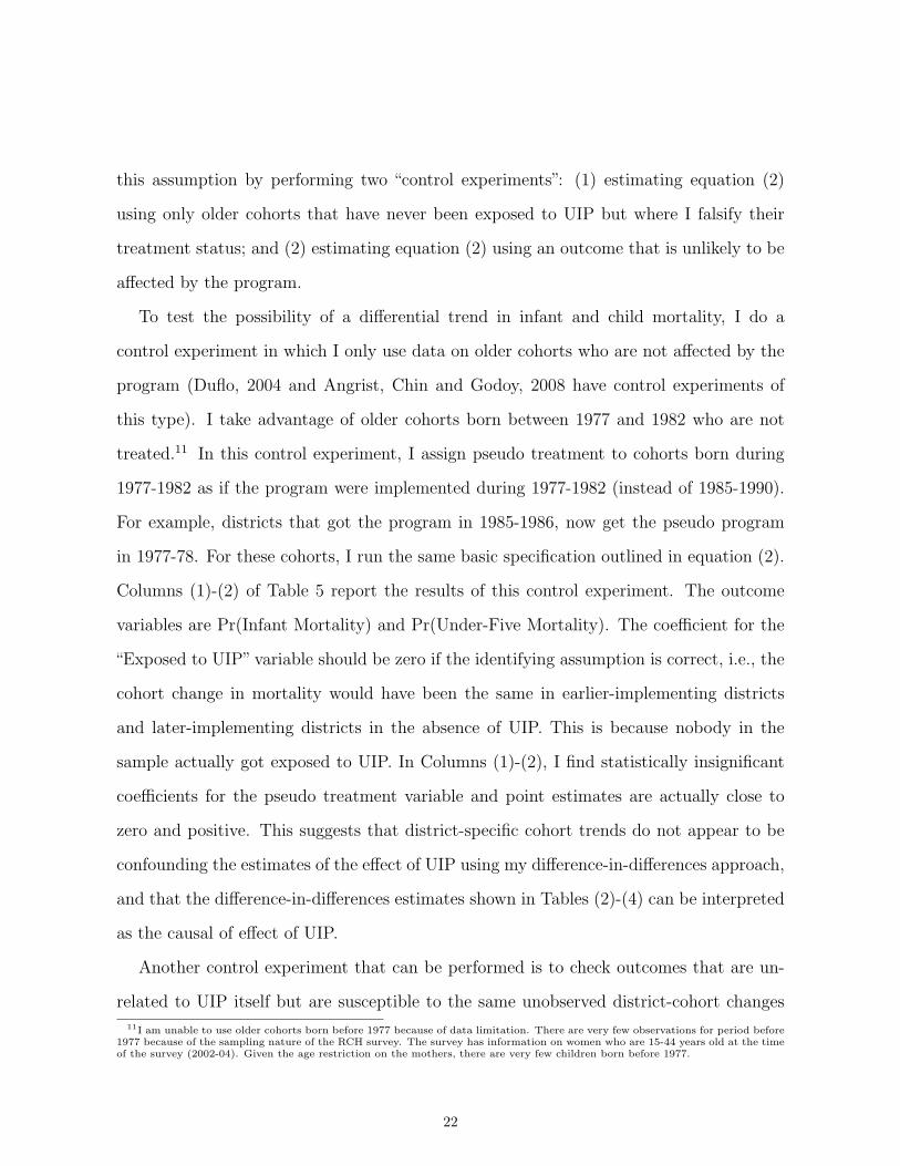
this assumption by performing two “control experiments”: (1) estimating equation (2)
using only older cohorts that have never been exposed to UIP but where I falsify their
treatment status; and (2) estimating equation (2) using an outcome that is unlikely to be
affected by the program.
To test the possibility of a differential trend in infant and child mortality, I do a
control experiment in which I only use data on older cohorts who are not affected by the
program (Duflo, 2004 and Angrist, Chin and Godoy, 2008 have control experiments of
this type). I take advantage of older cohorts born between 1977 and 1982 who are not
treated.11 In this control experiment, I assign pseudo treatment to cohorts born during
1977-1982 as if the program were implemented during 1977-1982 (instead of 1985-1990).
For example, districts that got the program in 1985-1986, now get the pseudo program
in 1977-78. For these cohorts, I run the same basic specification outlined in equation (2).
Columns (1)-(2) of Table 5 report the results of this control experiment. The outcome
variables are Pr(Infant Mortality) and Pr(Under-Five Mortality). The coefficient for the
“Exposed to UIP” variable should be zero if the identifying assumption is correct, i.e., the
cohort change in mortality would have been the same in earlier-implementing districts
and later-implementing districts in the absence of UIP. This is because nobody in the
sample actually got exposed to UIP. In Columns (1)-(2), I find statistically insignificant
coefficients for the pseudo treatment variable and point estimates are actually close to
zero and positive. This suggests that district-specific cohort trends do not appear to be
confounding the estimates of the effect of UIP using my difference-in-differences approach,
and that the difference-in-differences estimates shown in Tables (2)-(4) can be interpreted
as the causal of effect of UIP.
Another control experiment that can be performed is to check outcomes that are un-
related to UIP itself but are susceptible to the same unobserved district-cohort changes11I am unable to use older cohorts born before 1977 because of data limitation. There are very few observations for period before
1977 because of the sampling nature of the RCH survey. The survey has information on women who are 15-44 years old at the timeof the survey (2002-04). Given the age restriction on the mothers, there are very few children born before 1977.
22
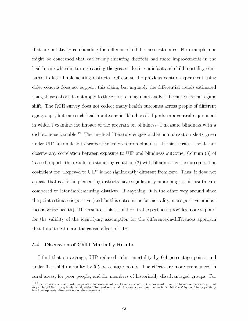
that are putatively confounding the difference-in-differences estimates. For example, one
might be concerned that earlier-implementing districts had more improvements in the
health care which in turn is causing the greater decline in infant and child mortality com-
pared to later-implementing districts. Of course the previous control experiment using
older cohorts does not support this claim, but arguably the differential trends estimated
using those cohort do not apply to the cohorts in my main analysis because of some regime
shift. The RCH survey does not collect many health outcomes across people of different
age groups, but one such health outcome is “blindness”. I perform a control experiment
in which I examine the impact of the program on blindness. I measure blindness with a
dichotomous variable.12 The medical literature suggests that immunization shots given
under UIP are unlikely to protect the children from blindness. If this is true, I should not
observe any correlation between exposure to UIP and blindness outcome. Column (3) of
Table 6 reports the results of estimating equation (2) with blindness as the outcome. The
coefficient for “Exposed to UIP” is not significantly different from zero. Thus, it does not
appear that earlier-implementing districts have significantly more progress in health care
compared to later-implementing districts. If anything, it is the other way around since
the point estimate is positive (and for this outcome as for mortality, more positive number
means worse health). The result of this second control experiment provides more support
for the validity of the identifying assumption for the difference-in-differences approach
that I use to estimate the causal effect of UIP.
5.4 Discussion of Child Mortality Results
I find that on average, UIP reduced infant mortality by 0.4 percentage points and
under-five child mortality by 0.5 percentage points. The effects are more pronounced in
rural areas, for poor people, and for members of historically disadvantaged groups. For12The survey asks the blindness question for each members of the household in the household roster. The answers are categorized
as partially blind, completely blind, night blind and not blind. I construct an outcome variable “blindnes” by combining partiallyblind, completely blind and night blind together.
23
example, children born into poor households were 0.9 percentage points less likely to die
within the first twelve months and 1.3 percentage points less likely to die within the first
five years. Thus, there are huge benefits of a mass immunization program in terms of
reducing child mortality.
As mentioned in section 3, these estimates may underestimate the true effect of UIP
for a couple of reasons. First, because consumption of vaccines has a positive externality,
it is possible that the control group benefits indirectly from UIP. Second, an immunization
program may provide more benefits in urban areas than has been estimated because prior
to UIP, some people in urban areas might have been vaccinated under the EPI program.
The dramatic effects on child mortality are consistent with children’s immune systems
being strengthened. This would suggest that there would be significant decreases in child
morbidity, too, due to UIP. Immunization not only protects against the specific diseases
(whose symptoms may be deadly to infants but only illness among older children) but also
improves the overall immune system of the body (which protects the children from other
illnesses). It is likely that the benefits of UIP on child health conditional on surviving
would not be confined to children from rural, low caste and poor households; children
from urban, higher caste and non-poor households may be far from the margin of survival
but there is still room for improvement in terms of health status. Unfortunately I do not
have the data to directly assess the effects of UIP on child health outcomes besides the
extreme outcome of mortality.13
It is worth highlighting that UIP has been a successful program in reducing child
mortality in India despite the fact that India is characterized by poor service delivery
mechanism and high absenteeism of health staffs. Banerjee, Deaton and Duflo (2004)
portray a very bleak picture of public and private health care provision in Udaipur district
of India and find that 45% of medical personnel are absent in health subcenters. A13The RCH survey has extensive health measures for children under age 5. Given that the RCH survey is collected in 2002-04,
all these children would have been exposed to UIP, leaving no variation in treatment. Thus these rich child health measures arenot usable for the purposes of estimating the impact of UIP.
24

similarly high level of absenteeism has also been found in a nationally representative
survey of primary health centers in India by Chaudhury et al. (2006). Despite these
impediments, the immunization program did achieve its intended objective of reducing
mortality among Indian children.
6 Effect of UIP on the Educational Outcomes of Surviving Chil-
dren
Some recent studies using plausibly exogenous variation in child health from inter-
ventions to reduce worm diseases and malaria and from school nutrition programs have
found a causal relationship running from child health to education (these were discussed
in subsection 2.2). In particular, improving child health improves educational outcomes.
The ability to attend school more regularly and often and to concentrate on studies better
when one is healthier is thought to be responsible at least in part. In the previous section,
I found that UIP reduced child mortality and speculate that it reduced child morbidity
too. Given these beneficial effects of UIP on child health, it is natural to ask what are
the consequences for the educational outcomes of the surviving children.
6.1 Estimation Results
Education results are based on children who survived beyond age five. Table 6 presents
the results of estimating equation (2) using each of the educational outcomes in turn-
Pr(Literate), Pr(Primary School Completion), Pr(Middle School Completion), Pr(Secondary
School Completion), and Years of Schooling.14 Column (1) suggests that the program has
no effect on the the probability of being literate. The educational outcomes are conditional
on child being literate.15 Column (2) suggests there is no significant effect of UIP on years
14I estimate these models using OLS, so in the case of a dichotomous outcome I am using the linear probability model. For thedichotomous outcomes, I have also used logit and find qualitatively similar results; these results are available upon request.
15The RCH survey asks for years of schooling completed only for people responding affirmatively to being literate. In theory, thiscould lead to selection bias when I examine the impact of UIP on years of schooling and the primary, middle and secondary schoolindicator variables since the sample is conditional on being literate. Therefore, I use the Heckman two-step correction method to
25

of schooling completed. This masks a nonlinear effect of UIP on schooling. UIP signifi-
cantly decreased the probability of primary school completion (by 4.6 percentage points),
had no impact on middle school completion and significantly increased the probability of
secondary school (by 1.9 percentage points).
Results in Table 6 suggest that though UIP did not raise years of schooling on average,
it reduced schooling at low levels of education and increased it at higher levels of education.
To get more detail on the effect of UIP at different points in the education distribution,
I estimate equation (2) for each level of schooling k, where the dependent variable is
Pr(Years of Schooling ≥ k), where k = 1 to 15. The estimated coefficients with the
95-percent confidence interval are plotted in Figure 1. Each point on the graph is from
a different regression. The “S” shape of Figure 1 suggests that the program decreased
the number of years of primary schooling for some children, but increased the number
of secondary schooling for others. At the low end, there is a shift away from completing
5 years of schooling toward completing 2-4 years of schooling. At the high end, there is
a shift away from completing fewer than ten years of schooling toward completing 10-12
years of schooling. Apparently the decrease at the lower end of the education distribution
offsets the gains at the upper end, leading to a zero average effect on years of schooling.
In Figure 2, I perform the same analysis as in Figure 1 but separately for children in
rural and urban areas. Comparing Panels A and B, we see that all the negative impact of
UIP at the low end of the education distribution is coming from rural areas-the graph in
Panel B is flat at zero for the first nine years of schooling. This is especially interesting
since it was only in rural areas where UIP had an impact on child mortality. UIP increased
schooling at the high end of the education distribution for children in both the urban and
rural areas, however.
In Figure 3, I perform the same analysis as in Figure 1 but separately for children
correct for the sample selection bias. In practice, the bias on the estimated effect of UIP is negligible given the insignificant resultin Column (1). In additional analysis, I have coded being illiterate as having zero years of schooling or at least less than primaryschool completion and all the results I am about to discuss remain.
26
from low, middle and high socio-economic status households. We see that all the negative
impact of UIP at the low end of the education distribution is coming from poor households-
the graph in Panels B and C does not have the trough at the lower levels of schooling. This
is also interesting because it was only in poor households where UIP significantly reduced
child mortality. The effects have an inverse U-shape at the high end of the education
distribution in all three wealth category though results are only significant for the poor
category.16
6.2 Channels for the Effect of UIP on Educational Outcomes
UIP had mixed impacts on children’s educational outcomes. It appears to have de-
creased the number of primary grades completed for some children but increased the
number of secondary grades completed for other children. This nonlinear effect in which
some children have worse educational outcomes and others have better ones is unusual
vis-a-vis the existing literature which has tended to find positive effects on education for
health interventions that improve child health. There are various explanations for the
results that I find in Table 6 and Figures 1-3. Though I cannot conclusively pin down the
pathways, here I describe several hypotheses consistent with the results. These hypotheses
are not mutually exclusive, and may each have a part in the overall results.
Change in the composition of the surviving pool of the children can be one factor that
is driving the nonlinear effects on education. First, UIP reduced child mortality. I will call
the children who UIP saved from dying marginal children. Though they are alive (and in
this sense, have better health than without UIP), these marginal children are probably
less healthy than the average child. Because they have worse health among surviving
children, they have worse educational outcomes. This may be because they attend school
less frequently, have less capacity to focus and learn, or take longer time to complete
normal tasks.16The lack of significance is likely because the number of observations is much less when I perform the analysis separately for
each SES category; results remain significant in Panel A because 45% of the sample is in the poor SES category.
27
As argued earlier, UIP also likely reduced child morbidity among inframarginal children
(i.e., the children far from the margin of survival). Since their health is better in the
traditional sense (i.e., as in the other papers estimating the causal impact of child health
on education such as Miguel and Kremer, 2004 and Bleakley, 2007), we might expect their
educational outcomes to improve as in these other papers.
That UIP improved health on two margins, from dying to survival for the children
on the margin of survival, from less healthy to more healthy for inframarginal children,
provides a cohesive story for the nonlinear effects on education. On the one hand, the
marginal children are likely to be concentrated on the lowest parts of the education distri-
bution, causing there an estimated reduction in primary school completion. Corroborating
this assertion is that in Figures 2 and 3, we observe a negative impact at the low end of the
education distribution only among those children who experienced a decline in mortality-
the rural and the poor. On the other hand, the inframarginal children are on higher parts
of the distribution and their improvement in health causes them to attain more years of
schooling.
Next, I discuss some of these other channels. The program effects on primary school
completion are far bigger than the effects on mortality and this suggests that additional
channels may be at work besides the change in composition of surviving children. One
is government resource constraints and bureaucratic inefficiency. In developing countries,
resources always compete with other strategies and interventions to raise the quality of
life. It is quite possible that there was a resource constraint and government’s financial and
human resources were more focused on the child health programs rather than schooling and
not enough resources were left for providing better school infrastructure. Resources spent
on child health programs may have crowded out resources for educational investments and
that, in turn, may have dampened the incentives for the teachers, thereby lowering school
quality. For example, teachers may not get salary at all or do not get it on time,17 there17Delayed salary is a common phenomena in developing countries.
28
can be fewer schools, classrooms, blackboards etc. In addition to government resource
constraints, bureaucratic inefficiency may have made the effects more severe. It is quite
possible that policy implementers focused more on UIP in order to achieve the yearly
targets of immunization coverage and were short-sighted about the effects on schooling
infrastructure. This may explain a part of the reduction in primary school completion.
Besides the government resource constraints story, there may be household resource
constraints that may be driving the negative effects. A second alternative explanation
for the negative effect of the UIP on primary school completion may be due to quality-
quantity tradeoff model where an unanticipated increase in household size due to the
immunization program induces the households to under-invest in each child. It may
be possible that UIP increased the number of surviving children,18forcing the resource
constraints households to invest less in the quality (education) of the children. But by
looking at the magnitudes of program effects on mortality and primary school completion,
it seems that quantity-quality tradeoff has a very small role in explaining the drop outs in
primary school. A third mechanism can be increased burden of sibling care in the family.
It is well documented and common in developing countries for the older siblings to stay
home to take care of younger siblings in the family. In this case, it is possible that the
older siblings and other children in the family who drop out of school to take care of the
new child in the family. It is reasonable to argue that the drop out behavior of these
siblings may be partly responsible for generating such a bigger effect on primary school
completion. The drop out of actual survivors can not explain such a big effect, though it
can be partly responsible.
A final hypothesis for the negative effect on primary school completion is that improving
child health may actually increase children’s labor force participation. It is quite likely
that when returns to schooling are low or if the family is credit constrained, children join
the agricultural field with their parents to support the family or they enter the child labor18Though I do not test this here, in a companion paper, I examine the impact of UIP on the fertility of the women and on the
number of surviving children.
29
market. If a child is somewhat healthy but not so healthy that he can earn much working,
he may be sent to school. When his health improves say due to UIP, he may become
healthy enough to work and therefore drop out of school.
As for the positive effects of UIP on secondary school completion, besides the story
where the health of the inframarginal children improves, another hypothesis is that UIP
has increased the life expectancy of children, causing parents to invest more in children’s
education because there is a longer period to collect the returns. Jayachandran and
Lleras-Muney (forthcoming) find empirical evidence in support of this hypothesis. This
hypothesis is unlikely to apply in the present case, though, because UIP primarily affects
the mortality of very young children. Conditional on surviving to age 5, children’s life
expectancy does not differ much with or without UIP. Yet, parents are likely not making
educational investment decisions before age 5 in most of India and given this, UIP should
not impact education through this mechanism. However, it is true that vaccinations
reduce morbidity at later ages even if mortality is largely unaffected, and this can add
up to meaningful differences in productive days between UIP-exposed children and other
children.
The foregoing are potential mechanisms through which UIP may have impacted edu-
cation and in future work I will empirically assess the contribution of each mechanisms.
7 Conclusion and Policy Implications
By using the phase-in feature of India’s Universal Immunization Program immuniza-
tion program and eligibility rules that only granted vaccinations to children up to twelve
months, I estimate the causal effect of UIP on children’s health and education outcomes.
I find that the program significantly reduces infant mortality and under-five mortality in
India. Contrary to the popular belief that India is plagued with inefficient program imple-
mentation capacity and poor public health service delivery system, this paper establishes
30

that UIP was successful in achieving its objective of reducing mortality.
Among surviving children, UIP had a negative impact on primary school completion
for some, but a positive impact on secondary school completion for others. The results
on education outcomes can be explained in terms of change in the composition of the
surviving children due to the immunization program. The negative effect at low levels
of schooling may be due to lower average health among marginal surviving children or
resource constraints faced by the government where investments in child health programs
may have crowded out investment in school infrastructure and quality. Increased burden
of siblings care can be another factor responsible for the negative effect on education. On
the other hand, the result that UIP increased the education of some children is likely due
to improved health among those children who are not at the margin of survival.
The results of this paper have important policy implications for the design of optimal
health and education policy in developing countries. While the program had the intended
benefit of increasing the survival probability of young children, there are mixed results
for educational outcomes with more children less likely to complete primary school. It
may be that resources of both government and families were too severely constrained to
meet the needs of the marginal children. A lesson may be that child health and education
policies have to be considered jointly so that children not only survive but are also given
adequate resources and opportunities to receive a decent education. Policymakers should
provide additional resources to educate the marginal child and help them perform better.
Provision of extra teacher similar to “balasakhi” would be a step forward in this direction
(Banerjee et al., 2007).
31
References
Aaby, P; Knudsen, K.; Samb, B and Simondon F. “ Non-Specific Beneficial Effect of MeaslesImmunisation: An Analysis of Mortality Studies from Developing Countries.”BritishMedical Journal, 2005, 311, pp. 481-5.
Alderman, Harold; Behrman Jere R.; Lavy, Victor and Menon, Rekha. “Child Health andSchool Enrolment: A Longitudinal Analysis.” Journal of Human Resources, 2001,36(1), pp. 185-205.
Angrist, Joshua; Lavy, Victor and Schlosser, Analia. “New Evidence on the Causal Linkbetween the Quantity and Quality of Children.” MIT Working Paper, 2005.
Angrist, Joshua; Chin, Aimee and Godoy, Ricardo. “Is Spanish-only Schooling responsi-ble for the Puerto Rican Language Gap?” Journal of Development Economics, 2008,85(1), pp. 105-128.
Annual Report. Ministry of Health and Family Welfare (MoHFW), 1987-88, Governmentof India.
Azarnert, Leonid V. “Child Mortality, Fertility, and Human Capital Accumulation.”Journalof Population Economics, 2006, 19, pp. 285-297.
Balakrishnan, T. R. “Effects of Child Mortality on Subsequent Fertility of Women in SomeRural and Semi-Urban Areas of Central Latin American Countries.”Population Stud-ies, 1978, 32, pp. 135-145.
Banerjee, Abhijit; Deaton, Angus and Duflo, Esther. “Wealth, Health, and Health Ser-vices in Rural Rajasthan.” American Economic Review, 2004, 94(2), pp. 326-330
Banerjee, Abhijit; Cole, Shawn; Duflo, Esther and Linden, Leigh L. “Remedying Educa-tion: Evidence from Two Randomized Experiments in India.” Quarterly Journalof Economics, 2007, 122(3), pp. 1235-1264.
Becker, Gary S. and Lewis, Gregg H. “On the Interaction between the Quantity and Qual-ity of Children.” Journal of Political Economy, 1973, 81(2), pp. S279-S288.
Behrman, Jere R. “The Impact of Health and Nutrition on Education.” World Bank Re-search Observer, 1996, 11(1), pp. 25-37.
Black, Sandra E.; Devereux Paul J. and Salvanes Kjell G. “The More the Merrier? TheEffect of Family Size and Birth Order on Children’s Education.” Quarterly Journalof Economics, 2005, 120(2), pp. 669-700.
Bleakley, Hoyt. “Disease and Development: Evidence from Hookworm Eradication in theAmerican South.” Quarterly Journal of Economics, 2007, 122(1). pp. 73-117.
Bleakley, Hoyt. “Malaria Eradication in the Americas: A Retrospective Analysis of Child-hood Exposure.” Working paper, CEDE/Los Andes, September 2006.
32
Bloom, David E.; Canning, David and Weston, Mark “The Value of Vaccination.” WorldEconomics, 2005, 6(3), July-Sep.
Bobonis, Gustavo J.; Miguel, Edward and Sharma, Charu P. “Iron Deficiency, Anemia andSchool Participation.” Journal of Human Resources, 2006, 41(4), pp.692-721.
Botezan, C. and Karmaus, W. “Does a higher number of siblings protect against the de-velopment of allergy and asthma? A review.” Journal of Epidemiology and Commu-nity Health, 2002 56, pp. 209-217.
Chaudhury, Nazmul; Hammer, J.; Kremer, M. and Muralidharan, K.; and Rogers, H. “Missingin Action: Teacher and Health Worker Absence in Developing Countries.” Journalof Economic Perspectives, Winter 2006, Vol. 20(1), pp. 91-116.
Chowdhary, A.K.M.A.; Khan, A. R. and Chen, L.C. “The Effect of Child Mortality onSubsequent Fertility in Pakistan and Bangladesh.” Population Studies, 1976, 2, pp.249-261.
Cutler, David; Fung, Winnie; Kremer, Michael and Singhal, Monica. “Mosquitoes: The Long-term Effects of Malaria Eradication in India.” NBER Working Paper No. 13539,2007.
Datar, Ashilesh; Mukherji, Anirban and Sood, Neeraj. “Health Infrastructure and Immu-nization Coverage in Rural India,”Indian Journal of Medical Research, 2007, January,pp. 31-42.
Donohue, John J. and Levitt, Steve. “The Impact of Legalized Abortion on Crime,”Quar-terly Journal of Economics, 2001, 116(2), pp. 379-420.
Glewwe, Paul and Jacoby, Hannan G. “An Economic Analysis of Delayed Primary SchoolEnrollment in a Low Income Country: The Role of Early Childhood Nutrition.”Review of Economic Statistics, 1995, 77(1), pp.156-169.
Glewwe, Paul; King, Elizabeth and Jacoby, Hannan G. (2001) , “Early Childhood Nutri-tion and Academic Achievement: A Longitudinal Analysis.” Journal of Public Eco-nomics, 2001, 81(3), pp. 345-368.
Glewwe, Paul and Miguel, Edward. “The Impact of Child Health and Nutrition on Edu-cation in Less Developed Countries.” Handbook of Development Economics, Volume4 (eds.) T. Paul Schultz and John Strauss, New York, NY: Elsevier, 2008, pp. 3561-3606.
Glewwe, Paul and Kremer, Michael. “Schools, Teachers, and Education Outcomes in De-veloping Countries.” Handbook of the Economics of Education, Volume 2, edited byEric A. Hanushek and Finis Welch. New York, NY: Elsevier, 2006, pp. 945-1017.
Gruber, Jonathan; Levine, Phillip B. and Staiger, Douglas. “Abortion Legalization and ChildLiving Circumstances: Who is the Marginal Child?”Quarterly Journal of Economics,1999, 114(1), 263-291.
33
Gupta, J.P. and Murali, Indira. “National Review of Immunization Programme in India.”1989, MoHFW, National Institute of Health and Family Welfare, New Delhi.
Jayachandran, Seema and Muney, Adrienne L. “Life Expectancy and Human Capital In-vestments: Evidence from Maternal Mortality Declines.” Quarterly Journal of Eco-nomics, forthcoming.
Kane, M. and Lasher, H. “The Case for Childhood Immunization.” Occasional Paper No.5, Children’s Vaccine Program at Path, Seattle, WA, 2002.
Koeing MA; Khan MA; Wojtynink B.; Clemens J.D. “The impact of measles vaccinationupon childhood mortality in Matlab, Bangladesh.” Bulletin of the World Health Or-ganization, 1990, 68, pp. 441-447.
Lucas, Adrienne M. “Economic Effects of Malaria Eradication: Evidence from the Malar-ial Periphery.” Mimeo, Brown University.
Miguel, Edward and Kremer, Michael. “Worms: Identifying Impacts on Education andHealth in the Presence of Treatment Externalities.”Econometrica, 2004, 72(1), pp.159-217.
Olsen, R. J. “Estimating the Effect of Child Mortality on the Number of Births.” Demog-raphy, 1980, 17, pp. 429-443.
Olsen, R. J. and Wolpin, K.I. “The Impact of Exogenous Child Mortality on Fertility: AWaiting Time Regression with Dyanamic Regressors”.Econometrica, 1983, 51, pp.731-749.
Oster, Emily. “Does Increased Access Increase Equality? Gender and Child health Invest-ments in India.” Journal of Development Economics, Forthcoming, 2008.
Palloni, A. and Rafalimanana, H. “The Effect of Infant Mortality on Fertility Revised:New Evidence from Latin America.” Demography, 1999, 36, pp. 41-58
Preston, S. H. “The Effect of Infant and Child Mortality on Fertility.” Academic, NewYork, 1978.
Rutstein, S. O. “The Influence of Child Mortality on Fertility in Taiwan.”Studies in Fam-ily Planning, 1974, 5, pp. 182-188
Sathyamala, C. “Immunization, The Technology Missions.”Seminar, 1989, 354, New Delhi,February.
World Health Organization (http://www.who.int).
Vermeersch, C. and Kremer, Michael. “School Meals, Educational Achievement and SchoolCompetition: Evidence from Randomized Evaluation.” Unpublished Working Paper,World Bank and Harvard University.
34

Table 1: Descriptive Statistics
Sample used in Child Sample used inMortality Analysis Education Analysis
Variables Mean S.D. Mean S.D.
Treated 0.75 (0.43) 0.67 (0.47)Rural 0.69 (0.46) 0.68 (0.46)Female 0.48 (0.50) 0.50 (0.50)Low SES 0.47 (0.50) 0.45 (0.50)Middle SES 0.31 (0.46) 0.32 (0.47)High SES 0.22 (0.41) 0.22 (0.42)ST 0.16 (0.37) 0.17 (0.37)SC 0.17 (0.38) 0.17 (0.37)OBC 0.38 (0.48) 0.37 (0.48)Hindu 0.76 (0.43) 0.74 (0.44)Muslim 0.13 (0.33) 0.14 (0.35)Christian 0.07 (0.25) 0.07 (0.25)Birth Order 2.37 (1.38)Mother Age 37.06 (3.95)Mother Literate 0.39 (0.49)Infant Mortality 0.09 (0.28)Under-five Mortality 0.11 (0.31)Literate 0.82 (0.39)Years of Schooling 6.15 (3.39)Primary School Completion 0.65 (0.48)Middle School Completion 0.36 (0.48)Secondary School Completion 0.18 (0.38)Age 13.71 (4.17)
Number of States and UTs 35 35Number of Districts 561 561Number of Observations 297,385 898,789
Notes: ST, SC and OBC are Scheduled Tribe, Scheduled Caste and Other Backward Caste respectively.
ST and SC are historically disadvantaged group. SES is socio-economic status of the households.
Different samples are used for the child mortality analysis and education analysis because the data
are from different file of the RCH survey. The paper uses information from the household file for education
analysis and information from fertility file for child mortality analysis. Household file has information
on all the individuals who live in the house, and from the household file one women is selected
(15-44 years) to be asked about her complete fertility history.
35
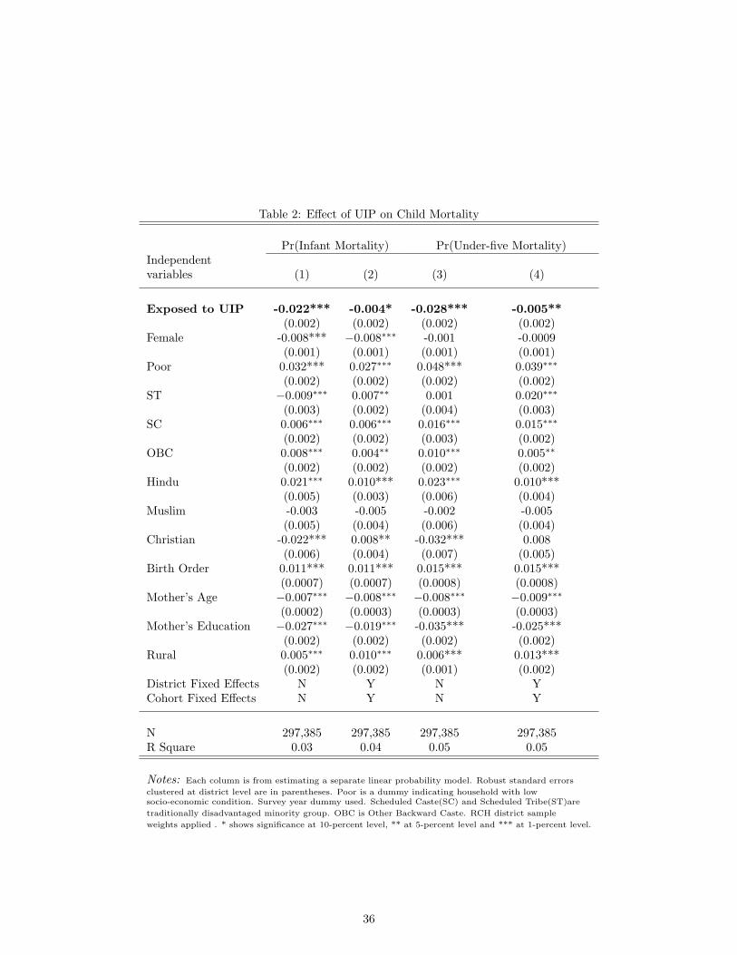
Table 2: Effect of UIP on Child Mortality
Pr(Infant Mortality) Pr(Under-five Mortality)Independentvariables (1) (2) (3) (4)
Exposed to UIP -0.022*** -0.004* -0.028*** -0.005**(0.002) (0.002) (0.002) (0.002)
Female -0.008*** −0.008∗∗∗ -0.001 -0.0009(0.001) (0.001) (0.001) (0.001)
Poor 0.032*** 0.027∗∗∗ 0.048*** 0.039∗∗∗
(0.002) (0.002) (0.002) (0.002)ST −0.009∗∗∗ 0.007∗∗ 0.001 0.020∗∗∗
(0.003) (0.002) (0.004) (0.003)SC 0.006∗∗∗ 0.006∗∗∗ 0.016∗∗∗ 0.015∗∗∗
(0.002) (0.002) (0.003) (0.002)OBC 0.008∗∗∗ 0.004∗∗ 0.010∗∗∗ 0.005∗∗
(0.002) (0.002) (0.002) (0.002)Hindu 0.021∗∗∗ 0.010*** 0.023∗∗∗ 0.010***
(0.005) (0.003) (0.006) (0.004)Muslim -0.003 -0.005 -0.002 -0.005
(0.005) (0.004) (0.006) (0.004)Christian -0.022*** 0.008** -0.032*** 0.008
(0.006) (0.004) (0.007) (0.005)Birth Order 0.011*** 0.011*** 0.015*** 0.015***
(0.0007) (0.0007) (0.0008) (0.0008)Mother’s Age −0.007∗∗∗ −0.008∗∗∗ −0.008∗∗∗ −0.009∗∗∗
(0.0002) (0.0003) (0.0003) (0.0003)Mother’s Education −0.027∗∗∗ −0.019∗∗∗ -0.035*** -0.025***
(0.002) (0.002) (0.002) (0.002)Rural 0.005∗∗∗ 0.010∗∗∗ 0.006*** 0.013***
(0.002) (0.002) (0.001) (0.002)District Fixed Effects N Y N YCohort Fixed Effects N Y N Y
N 297,385 297,385 297,385 297,385R Square 0.03 0.04 0.05 0.05
Notes: Each column is from estimating a separate linear probability model. Robust standard errors
clustered at district level are in parentheses. Poor is a dummy indicating household with lowsocio-economic condition. Survey year dummy used. Scheduled Caste(SC) and Scheduled Tribe(ST)are
traditionally disadvantaged minority group. OBC is Other Backward Caste. RCH district sample
weights applied . * shows significance at 10-percent level, ** at 5-percent level and *** at 1-percent level.
36
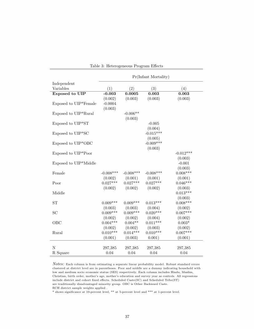
Table 3: Heterogeneous Program Effects
Pr(Infant Mortality)
IndependentVariables (1) (2) (3) (4)Exposed to UIP -0.003 0.0005 0.003 0.003
(0.002) (0.003) (0.003) (0.003)Exposed to UIP*Female -0.0004
(0.003)Exposed to UIP*Rural -0.006**
(0.003)Exposed to UIP*ST -0.005
(0.004)Exposed to UIP*SC -0.015***
(0.005)Exposed to UIP*OBC -0.009***
(0.003)Exposed to UIP*Poor -0.012***
(0.003)Exposed to UIP*Middle -0.001
(0.003)Female -0.008*** -0.008*** -0.008*** 0.008***
(0.002) (0.001) (0.001) (0.001)Poor 0.027*** 0.027*** 0.027*** 0.046***
(0.002) (0.002) (0.002) (0.003)Middle 0.013***
(0.003)ST 0.009*** 0.009*** 0.013*** 0.008***
(0.003) (0.003) (0.004) (0.002)SC 0.009*** 0.009*** 0.020*** 0.007***
(0.002) (0.002) (0.004) (0.002)OBC 0.004*** 0.004** 0.011*** 0.003*
(0.002) (0.002) (0.003) (0.002)Rural 0.010*** 0.014*** 0.010*** 0.007***
(0.001) (0.003) 0.001) (0.001)
N 297,385 297,385 297,385 297,385R Square 0.04 0.04 0.04 0.04
Notes: Each column is from estimating a separate linear probability model. Robust standard errors
clustered at district level are in parentheses. Poor and middle are a dummy indicating household with
low and medium socio economic status (SES) respectively. Each column includes Hindu, Muslim,
Christian, birth order, mother’s age, mother’s education and survey year as controls. All regressions
include district and cohort fixed effects. Scheduled Caste(SC) and Scheduled Tribe(ST)
are traditionally disadvantaged minority group. OBC is Other Backward Caste.
RCH district sample weights applied .
* shows significance at 10-percent level, ** at 5-percent level and *** at 1-percent level.
37
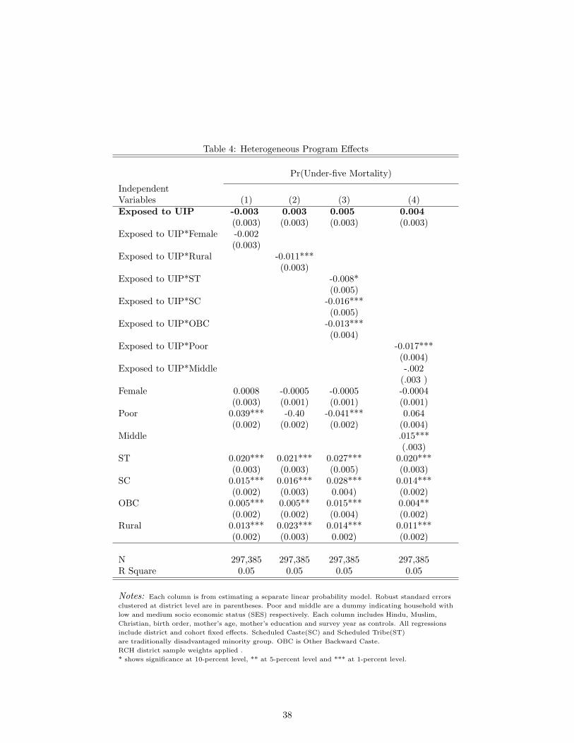
Table 4: Heterogeneous Program Effects
Pr(Under-five Mortality)
IndependentVariables (1) (2) (3) (4)Exposed to UIP -0.003 0.003 0.005 0.004
(0.003) (0.003) (0.003) (0.003)Exposed to UIP*Female -0.002
(0.003)Exposed to UIP*Rural -0.011***
(0.003)Exposed to UIP*ST -0.008*
(0.005)Exposed to UIP*SC -0.016***
(0.005)Exposed to UIP*OBC -0.013***
(0.004)Exposed to UIP*Poor -0.017***
(0.004)Exposed to UIP*Middle -.002
(.003 )Female 0.0008 -0.0005 -0.0005 -0.0004
(0.003) (0.001) (0.001) (0.001)Poor 0.039*** -0.40 -0.041*** 0.064
(0.002) (0.002) (0.002) (0.004)Middle .015***
(.003)ST 0.020*** 0.021*** 0.027*** 0.020***
(0.003) (0.003) (0.005) (0.003)SC 0.015*** 0.016*** 0.028*** 0.014***
(0.002) (0.003) 0.004) (0.002)OBC 0.005*** 0.005** 0.015*** 0.004**
(0.002) (0.002) (0.004) (0.002)Rural 0.013*** 0.023*** 0.014*** 0.011***
(0.002) (0.003) 0.002) (0.002)
N 297,385 297,385 297,385 297,385R Square 0.05 0.05 0.05 0.05
Notes: Each column is from estimating a separate linear probability model. Robust standard errors
clustered at district level are in parentheses. Poor and middle are a dummy indicating household with
low and medium socio economic status (SES) respectively. Each column includes Hindu, Muslim,
Christian, birth order, mother’s age, mother’s education and survey year as controls. All regressions
include district and cohort fixed effects. Scheduled Caste(SC) and Scheduled Tribe(ST)
are traditionally disadvantaged minority group. OBC is Other Backward Caste.
RCH district sample weights applied .
* shows significance at 10-percent level, ** at 5-percent level and *** at 1-percent level.
38
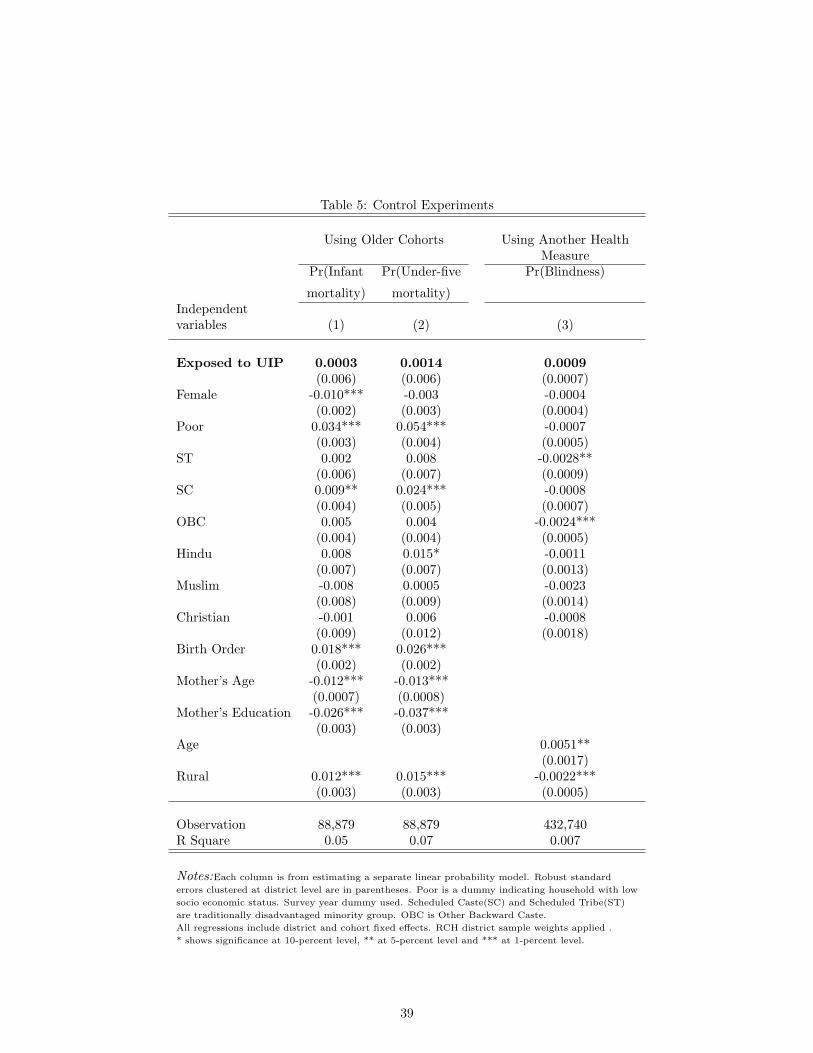
Table 5: Control Experiments
Using Older Cohorts Using Another HealthMeasure
Pr(Infant Pr(Under-five Pr(Blindness)
mortality) mortality)Independentvariables (1) (2) (3)
Exposed to UIP 0.0003 0.0014 0.0009(0.006) (0.006) (0.0007)
Female -0.010*** -0.003 -0.0004(0.002) (0.003) (0.0004)
Poor 0.034*** 0.054*** -0.0007(0.003) (0.004) (0.0005)
ST 0.002 0.008 -0.0028**(0.006) (0.007) (0.0009)
SC 0.009** 0.024*** -0.0008(0.004) (0.005) (0.0007)
OBC 0.005 0.004 -0.0024***(0.004) (0.004) (0.0005)
Hindu 0.008 0.015* -0.0011(0.007) (0.007) (0.0013)
Muslim -0.008 0.0005 -0.0023(0.008) (0.009) (0.0014)
Christian -0.001 0.006 -0.0008(0.009) (0.012) (0.0018)
Birth Order 0.018*** 0.026***(0.002) (0.002)
Mother’s Age -0.012*** -0.013***(0.0007) (0.0008)
Mother’s Education -0.026*** -0.037***(0.003) (0.003)
Age 0.0051**(0.0017)
Rural 0.012*** 0.015*** -0.0022***(0.003) (0.003) (0.0005)
Observation 88,879 88,879 432,740R Square 0.05 0.07 0.007
Notes:Each column is from estimating a separate linear probability model. Robust standard
errors clustered at district level are in parentheses. Poor is a dummy indicating household with low
socio economic status. Survey year dummy used. Scheduled Caste(SC) and Scheduled Tribe(ST)
are traditionally disadvantaged minority group. OBC is Other Backward Caste.
All regressions include district and cohort fixed effects. RCH district sample weights applied .
* shows significance at 10-percent level, ** at 5-percent level and *** at 1-percent level.
39
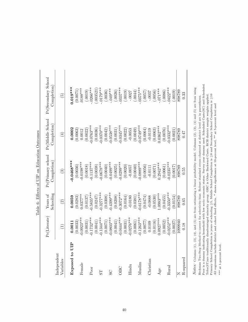
Tab
le6:
Effe
cts
ofU
IPon
Edu
cati
onO
utco
mes
Pr(
Lit
erat
e)Y
ears
ofP
r(P
rim
ary
scho
olP
r(M
iddl
eSc
hool
Pr(
Seco
ndar
ySc
hool
Scho
olin
gC
ompl
etio
n)C
ompl
etio
n)C
ompl
etio
n)In
depe
nden
tV
aria
bles
(1)
(2)
(3)
(4)
(5)
Expos
edto
UIP
0.00
110.
0059
-0.0
468*
**0.
0002
0.01
9***
(0.0
033)
(0.0
283)
(0.0
036)
(0.0
063)
(0.0
071)
Fem
ale
-0.0
923*
**0.
0377
**-0
.019
8***
0.00
12.0
188*
**(0
.003
1)(0
.013
7)(0
.001
8)(0
.002
2)(.
0019
)P
oor
-0.1
732*
**-0
.583
5***
-0.1
137*
**-0
.076
3***
-.02
66**
*(0
.004
1)(0
.024
7)(0
.003
8)(0
.003
6)(.
0035
21)
ST-0
.134
4***
-0.3
277*
**-0
.067
8***
-0.0
370*
**-.
0179
***
(0.0
071)
(0.0
308)
(0.0
040)
(0.0
042)
(.00
36)
SC-0
.080
3***
-0.4
399*
**-0
.049
9***
-0.0
538*
**-.
049*
**(0
.004
1)(0
.020
8)(0
.002
5)(0
.003
1)(.
0026
)O
BC
-0.0
444*
**-0
.307
2***
-0.0
299*
**-0
.034
5***
-.03
37**
*(0
.003
1)(0
.016
4)(0
.002
0)(0
.002
2)(.
0019
)H
indu
-0.0
276*
**-0
.018
0-0
.005
7-0
.005
3-.
0027
(0.0
061)
(0.0
381)
(0.0
040)
(0.0
049)
(.00
44)
Mus
lim-0
.126
3***
-0.6
178*
**-0
.088
9***
-0.0
749*
**-.
0375
***
(0.0
077)
(0.0
474)
(0.0
056)
(0.0
064)
(.00
57)
Chr
isti
an0.
0109
-0.0
888
-0.0
111
-0.0
119
-.003
7(0
.011
6)(0
.053
0)(0
.007
1)(0
.006
3)(.
0056
)A
ge0.
0927
***
1.09
83**
*0.
2942
***
0.03
62**
*-.
071*
**(0
.005
2)(0
.045
5)(0
.006
1)(0
.007
6)(.
0086
)R
ural
-0.0
252*
**-0
.335
0***
-0.0
235*
**-0
.033
2***
-.04
22**
*(0
.002
7)(0
.015
4)(0
.001
7)(0
.002
1)(.
0019
)N
1099
940
8987
8989
8789
8987
8989
8789
R-s
quar
ed0.
180.
650.
550.
470.
33
Not
es:
Colu
mns
(1),
(3),
(4),
and
(5)
are
from
est
imati
ng
alinear
pro
babilit
ym
odel.
Colu
mns
(2),
(3),
(4)
and
(5)
are
from
usi
ng
Heck
man
Tw
o-S
tep
Meth
od
tocorr
ect
for
sele
cti
vit
y-b
ias.
Robust
standard
err
ors
clu
stere
dat
dis
tric
tle
vel
are
inpare
nth
ese
s.
Poor
isa
dum
my
indic
ati
ng
house
hold
wit
hlo
wso
cio
econom
icst
atu
s.Surv
ey
year
dum
my
use
d.
Sch
edule
dC
ast
e(S
C)
and
Sch
edule
d
Tri
be(S
T)a
retr
adit
ionally
dis
advanta
ged
min
ori
tygro
up.
OB
Cis
Oth
er
Back
ward
Cast
e.
RC
Hdis
tric
tsa
mple
weig
hts
applied.
Pri
mary
Sch
ool
Com
ple
tion
isyears
of
schooling≥
5,
Mid
dle
Sch
ool
Com
ple
tion
is≥
8and
Secondary
Sch
ool
Com
ple
tion
is≥
10
All
regre
ssio
ns
inclu
de
dis
tric
tand
cohort
fixed
eff
ects
.*
show
ssi
gnifi
cance
at
10-p
erc
ent
level,
**
at
5-p
erc
ent
level
and
***
at
1-p
erc
ent
level.
40
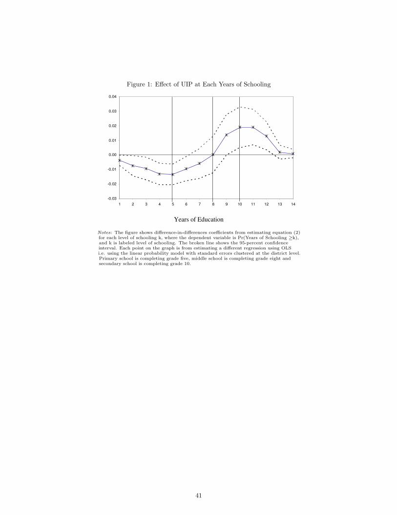
Figure 1: Effect of UIP at Each Years of Schooling
-0.03
-0.02
-0.01
0.00
0.01
0.02
0.03
0.04
1 2 3 4 5 6 7 8 9 10 11 12 13 14
Years of Education
Notes: The figure shows difference-in-differences coefficients from estimating equation (2)for each level of schooling k, where the dependent variable is Pr(Years of Schooling ≥k),and k is labeled level of schooling. The broken line shows the 95-percent confidenceinterval. Each point on the graph is from estimating a different regression using OLSi.e. using the linear probability model with standard errors clustered at the district level.Primary school is completing grade five, middle school is completing grade eight andsecondary school is completing grade 10.
41
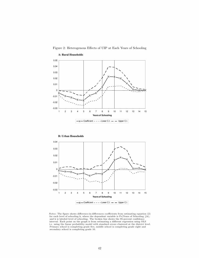
Figure 2: Heterogenous Effects of UIP at Each Years of Schooling
A: Rural Households
-0.03
-0.02
-0.01
0
0.01
0.02
0.03
0.04
0.05
1 2 3 4 5 6 7 8 9 10 11 12 13 14 15
Years of Schooling
Coefficient Lower C.I. Upper C.I.
B: Urban Households
-0.03
-0.02
-0.01
0
0.01
0.02
0.03
0.04
1 2 3 4 5 6 7 8 9 10 11 12 13 14 15
Years of Schooling
Coefficient Lower C.I. Upper C.I.
Notes: The figure shows difference-in-differences coefficients from estimating equation (2)for each level of schooling k, where the dependent variable is Pr(Years of Schooling ≥k),and k is labeled level of schooling. The broken line shows the 95-percent confidenceinterval. Each point on the graph is from estimating a different regression using OLSi.e. using the linear probability model with standard errors clustered at the district level.Primary school is completing grade five, middle school is completing grade eight andsecondary school is completing grade 10.
42
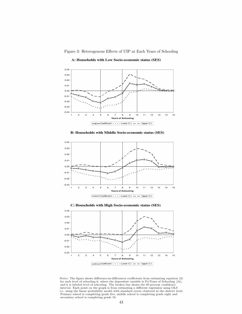
Figure 3: Heterogenous Effects of UIP at Each Years of Schooling A: Households with Low Socio-economic status (SES)
-0.04
-0.03
-0.02
-0.01
0.00
0.01
0.02
0.03
0.04
1 2 3 4 5 6 7 8 9 10 11 12 13 14 15
Years of Schooling
Coefficient Lower C.I. Upper C.I.
B: Households with Middle Socio-economic status (SES)
-0.03
-0.02
-0.01
0.00
0.01
0.02
0.03
0.04
1 2 3 4 5 6 7 8 9 10 11 12 13 14 15
Years of Schooling
Coefficient Lower C.I. Upper C.I.
C: Households with High Socio-economic status (SES)
-0.03
-0.02
-0.01
0.00
0.01
0.02
0.03
0.04
1 2 3 4 5 6 7 8 9 10 11 12 13 14 15
Years of Schooling
Coefficient Lower C.I. Upper C.I.
Notes: The figure shows difference-in-differences coefficients from estimating equation (2)for each level of schooling k, where the dependent variable is Pr(Years of Schooling ≥k),and k is labeled level of schooling. The broken line shows the 95-percent confidenceinterval. Each point on the graph is from estimating a different regression using OLSi.e. using the linear probability model with standard errors clustered at the district level.Primary school is completing grade five, middle school is completing grade eight andsecondary school is completing grade 10.
43

Appendix
Symptoms of the Disease
Table 1: Symptoms of the Disease
Diseases Symptoms Vaccines
Diphtheria Sore throat and fever, Contagious DPTChildren under age 5 are at risk
Pertussis Malnutrition, Pneumonia DPT
Tetanus Lock Jaw, Muscles Pain DPT
Polio Viral fever, Paralysis Oral Polio
Measles Skin rash, Running nose and Red eye Measle
Tuberculosis Chest pain, Coughing up blood BCGFever, Weight Loss and Appetite Loss
Treatment takes 6-12 months
Immunization Schedule
Table 2: Immunization Schedule
Age of the ChildAt Birth 6 Weeks 12 weeks 16 Weeks 9-12 months
Primary Vaccination:
BCG YesOral Polio Yes Yes Yes
DPT Yes Yes YesMeasles Yes
44

Exposure to the Program
Table 3: Exposure to the Program by Year of Birth and UIP Year
UIP Year
Year of Birth 1986 1987 1988 1989 1990
1982198319841985 Yes1986 Yes Yes1987 Yes Yes Yes1988 Yes Yes Yes Yes1989 Yes Yes Yes Yes Yes1990 Yes Yes Yes Yes Yes1991 Yes Yes Yes Yes Yes
Number of Districts 48 92 112 136 175 563
Table 3 explains the variations in exposure to the program across cohorts and across districts. Staggeredimplementation of the program across districts between 1986-1990 led to differences in exposure to the programfor children within the same birth cohorts. The official eligibility rule of getting all the eight vaccines before theage of 12 months results in difference in exposure to the program across cohorts. Children are exposed to theprogram if their year of birth is either before and one year after their district of birth got the program. Forexample, children born in 1987 are treated if they were born in districts which got the program either before1987 or one year after i.e. 1988 whereas children born in 1987 are considered untreated if they were born indistricts which got the program in years later than 1988 (e.g. 1989, 1990). This illustrates that same birth cohortare exposed differently to the program depending on when their district got the program. This is variation inexposure to the program across district. Also, within a district different birth cohorts are exposed differently tothe program. Cohorts who are older than one year when the program was placed in their district are not exposedto the program whereas cohorts who are younger than one year when the program was placed in their district areexposed to the program. This is variation in exposure to the program across cohort.
45
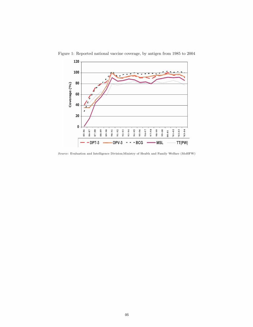
Figure 1: Reported national vaccine coverage, by antigen from 1985 to 2004
Source: Evaluation and Intelligence Division;Ministry of Health and Family Welfare (MoHFW)
46
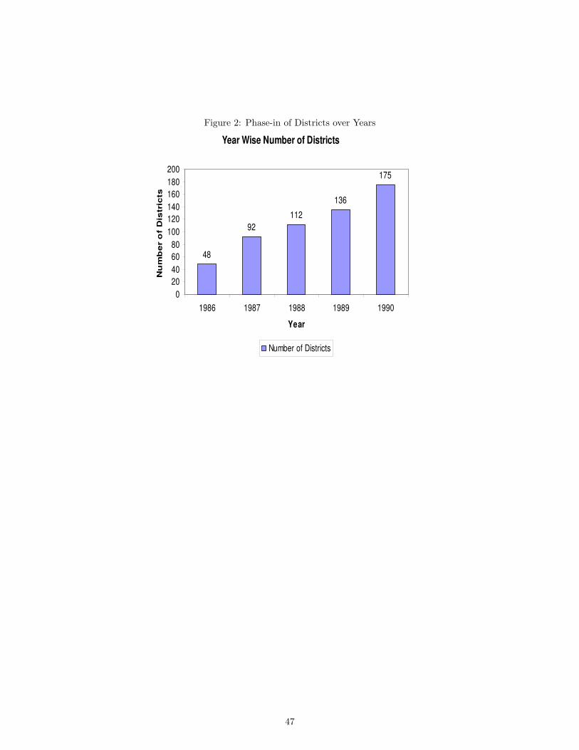
Figure 2: Phase-in of Districts over Years
Year Wise Number of Districts
48
92
112
136
175
0
20
40
60
80
100
120
140
160
180
200
1986 1987 1988 1989 1990
Year
Nu
mb
er o
f D
istric
ts
Number of Districts
47
Top Related