


Languages
Pages
Legal

Charge transparencies and amplification properties of
Integrated Micromegas detectors
Maximilien Chefdeville
NIKHEF, Amsterdam
RD51, Amsterdam 17/04/2008

Overview
• InGrid, an integrated Micromegas
• Charge transparencies– Electron collection– Ion backflow
• Amplification properties in Ar-iC4H10 mixtures– Measuring Fano factors with the Timepix chip– Mean energies per ion pair– Gas gain– Energy resolution and gain fluctuations

InGrid, an integrated Micromegas for pixel readout gas detectors
• Solve alignment / pillar Ø / pitch issues of Micromegas pixel detectors by integrating the grid onto the chip
• Wafer post-processing– Grid geometry fits the chip– Pillar Ø ~ 30 μm
• Very good grid flatness– Gain homogeneity– Very good resolution
2 cm Ø
11.7 % FWHM @ 5.9 keV in P10
pillar
2 cm Ø

Electron collection studies

Electron collection• Micromegas basics
– Funnel of field lines at the hole entrances
– Compression factor is equal to the field ratio FR:SA = SD.ED/EA = SD / FR
– For FR>FR*, all field lines are transmitted to the amplification region SA
SD
EDrift
EAmplif.
Ion drift lines
Obviously, FR* depends on the grid optical transparency
Dependence on the hole pitch and the hole diameter
Also, the electrons don’t follow exactly the field lines
Dependence on the gas mixture

Electron collection• Measurements
– 55Fe 5.9 keV source– Prototypes:
• 20-58 μm hole pitch• 10-45 μm hole diameter
– Pocket MCA Amptek– Constant grid voltage, vary ED
• Lowering of the gain with ED
• Grid geometry study:– Ar 5% iC4H10
– FR* ↓ with the grid optical transparency
• Gas study:– Ar/CO2 5/95 10/90 20/80 and “pure” Ar– FR* ↑ with the electron temperature

Ion backflow studies

Ion backflow in Micromegas• First studies performed by Saclay/Orsay
I. Giomataris, V. Lepeltier, P. ColasNucl. Instr. and Meth. A 535 (2004) 226
• Intrinsic low BF as most of the field lines in the avalanche gap end on the grid
• Number of ions arriving on the grid depends on:
– Shape/size of the field line funnel– Ion formation positions
• Shape/size of the field line funnel– Grid geometry– Ratio of the Amplification to Drift fields
• Ion formation positions– Longitudinally: Townsend coefficient– Transversally: Electron diffusion
Ion drift lines
Electron avalanches
EDrift
EAmplif.

Experimental set-up• X-ray gun up to 12 keV photons, 200 μA
– Operated at 9 keV energy (50 μA)• 10 keV photo e- range ~ 1 cm in Ar
– Collimator is 2 cm thick with a 3 mm Ø hole
• Guard electrode 1 mm above the grid– Adjustable voltage
• Cathode/Anode current measurements– Voltage drop through 92 MΩ resistor
Zinput = 1 GΩ, ΔI = 1 pA– Voltage drop through 10 MΩ resistor
Zinput = 100 MΩ, ΔI = 100 pA
• Reversed polarities:– Cathode at ground, grid and anode
at positive voltages– No field between detector window
and cathode
• Gas mixture: Ar:CH4 90:10

Experimental set-up
Electronics
Voltmeters
X-tube
Gas chamber
Collimator

Detector geometries4 different hole pitches
20, 32, 45 and 58 μm
20 & 32 μm pitch grids have pillars inside holes45 & 58 μm pitch grids have pillars between holes
3 different amplification gap thicknesses
– 45, 58 and 69 μm ± 1 μm– Operated at 325, 350 and 370 V– Amplification fields of 72, 60 and 53 kV/cm
Gains of 200, 550 and 150Diffusion coef. of 142, 152 and 160 μm/√cmAvalanche width of 9.5, 11.6 and 13.4 μm

Measurements in Ar:CH4 90:10• Vary field ratio FR from 100 to 1000
– Drift field from ~ 500 V/cm down to few ~ 50 V/cm– At high FR (low Drift field), primary e- loss due to field distortions
Stop at FR ~ 1000
• Fit curve with BF = p0/FRp1

Measurements with 45 μm gap InGrids
Gain ~ 200σt = 9.5 μm
20 μm pitch p1 = 1.0132 μm pitch p1 = 0.9045 μm pitch p1 = 0.9658 μm pitch p1 = 1.19
BF = p0/FRp1
At given field ratio and ion distribution, the backflow fraction ↓ with the pitch

Measurements with 58 μm gap InGrids
Gain ~ 500σt = 11.6 μm
20 μm pitch p1 = 1.0832 μm pitch p1 = 1.0245 μm pitch p1 = 1.0158 μm pitch p1 = 1.21
BF = p0/FRp1
BF < 1 ‰
At given field ratio and ion distribution, the backflow fraction ↓ with the pitch

Measurements with 70 μm gap InGrids
BF = p0/FRp1
Gain ~ 150σt = 13.4 μm
32 μm pitch p1 = 1.1445 μm pitch p1 = 1.1358 μm pitch p1 = 1.28
BF < 1 ‰
At given field ratio and ion distribution, the backflow fraction ↓ with the pitch

Summary of the measurements
At given field ratio, the backflow fraction ↓ with the ion distribution widthand ↑ with the hole pitch

Primary statistics and amplification properties

Measuring Fano factors with Gridpix
• Detect individual electrons from 55Fe
R2 = (F+b)/N + (1-η)/ηNF: Fano factor√b: single e- gain distribution rms (%)η: detection efficiencyN: number of primary e-
Raw spectrum
Access to F if efficiency η is known
b=0
Measure the primary statistics Mean energy per ion pair W
Fano factor F

Detection efficiency • Electron detected if its avalanche
is higher than the pixel threshold
threshold
Detection efficiency:
η = ∫t∞ p(g).dg
• Exponential fluctuations:p(g) = 1/<g> . exp (-g/<g>)η(g) = exp (-t/<g>)
• “Polya” fluctuations:parameter m=1/b with √b the relative rmsp(m,g) = mm/Γ(m) . 1/<g> . (g/<g>)m-1
. exp (-m.g/<g>)p(2,g) = 4 . 1/<g> . g/<g> . exp (-2.g/<g>)η(2,g) = (1+2.t/<g>) . exp(-2.t/<g>)

Experimental setup• Gas chamber
– Timepix chip15 μm SiProt + 50 μm InGrid
– 10 cm drift gap– Cathode strips and Guard electrode– Ar 5 % iC4H10
• 55Fe source placed on top– Collimated to 2 mm Ø beam– Difficult to align precisely
• Ideally, gain & threshold homogeneous– Pixel to pixel threshold variations
Threshold equalization provides uniform response– Gain homogeneity should be OK thanks to:
Amplification gap constant over the chip (InGrid)Amplification gap close to optimum
• Imperative: have enough diffusion to perform counting– Long drift length, look at escape peak– However: SiProt layer induces charge on neighboring pixels
500 V/cm
chip guard
strips
55Fe 5.9 & 6.5 keV
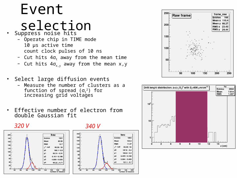
Event selection• Suppress noise hits
– Operate chip in TIME mode10 μs active timecount clock pulses of 10 ns
– Cut hits 4σt away from the mean time– Cut hits 4σx,y away from the mean x,y
• Select large diffusion events– Measure the number of clusters as a
function of spread (σt2) for increasing grid
voltages
• Effective number of electron from double Gaussian fit320 V 340 V

Collection efficiency• Data points: ne(Vg) = η(Vg).n0
• Analytical form of η(g) known for exponential and Polya fluctuations
• Use gain parameterization:g(Vg) = A.exp(B.Vg)A depends on the absolute gainB ~ 3-4.10-2 for Ar/iC4H10 mixtures
• Exponential fluctuations:n0 = 116.4 ± 2.8B = 5.15.10-2 ± 0.52.10-2
Polya fluctuations with m=2:n0 = 114.6 ± 2.6B = 3.35.10-2 ± 0.32.10-2
Mean energy per ion pairW = 3000 /114.6 = 26.2 ± 0.5 eV

At 350V…
RMSt = 6.25 %
η = 0.93
RMSη = 2.56 %
RMSp = 5.70 %
F = 0.35

Extending knowledge of W to other Ar/iso gas mixtures
• W constant above 1 keV– No matter the X-ray energy, same
energy fraction is spent in ionization
• Generate measurable primary currents (X-tube)
– Primary current depends on W and absorption coefficient
• Start with Ar and progressively introduce iso
– Check that the absorption does not change when introducing isobutane
Iso fraction (%) W (eV) Np (5.9 keV)
0 26.9 220
1 25.1 235
2.5 25.7 230
5 26.2 225
10 27.8 212
20 32.9 179

Gas gain curves in Ar/iso mixtures• Gas gain measured with an 55Fe source
– Penning transfers from Ar excited states to isobutane molecules– Cooling of the electrons at increasing isobutane concentration

Energy resolution in Ar/iso mixtures• General trend
– Resolution improves from gains of few 102 to few 103
– Degradation above few 103 Minima of resolution:Ar 2.5 % iC4H10:16 % FWHMAr 20 % iC4H10:14 % FWHM
FWHM Ratio = 1.14
√W ratio = 1.13
Gain fluctuations
F = 0.35
R = 6% RMS
b = 0.5 (m=2)
√b ~ 71 %

Conclusions
• Charge transparencies– Electron collection efficiency well understood– Ion backflow fractions in agreement with ones measured with
standard Micromegas
• Counting electrons from 55Fe with Timepix in Ar 5% iC4H10
– W = 26.2 eV– F = 0.35
• Gas gain fluctuations obey a Polya distribution with m=2, i.e. relative fluctuations of 71 %

Thanks for your attention
Thanks to all people from the NIKHEF/Twente/Saclay
pixel collaboration
Top Related