


Languages
Pages
Legal

Characterization and molecular dynamic studies of chitosan–ironcomplexes
T FAHMY1,2,* and A SARHAN2
1 Physics Department, College of Science and Humanities, Prince Sattam Bin Abdulaziz University, 11942 Al-Kharj,
Kingdom of Saudi Arabia2 Polymer Research Group, Physics Department, Faculty of Science, Mansoura University, Mansoura 35516, Egypt
*Author for correspondence ([email protected])
MS received 6 November 2020; accepted 14 December 2020
Abstract. Chitosan–iron (Cs–Fe) complexes are prepared electrochemically in an aqueous acidic medium in one-
compartment cell at different times. XRD pattern of Cs–Fe complex samples has been investigated in the range from 5� to
50� and revealed that chitosan is characterized by certain crystalline peaks at 8.73�, 11.92� and 18.96�. In addition, the
crystallinity of Cs–Fe complex samples is increased with increasing the content of Fe3?. Ultraviolet–visible (UV–Vis) and
Fourier transform-infrared (FTIR) spectroscopies have been used to investigate the optical properties of Cs–Fe complex
samples. UV analysis showed that pure chitosan is characterized by absorption band at 214 nm resulted from the amide
linkages and at 311 nm, as a shoulder which is attributed to intraligand n ? p and p ? p* transitions of the chro-
mophoric C=O group. On the other hand, two new bands are observed in Cs–Fe complex samples at nearly 350 and 389
nm with increasing Fe3? content. The optical parameters of all the samples, such as optical band gap energy (Eg), Urbach
energy (EU), dispersion energy (Ed) and oscillator energy (Eo) have been estimated. It is found that these parameters are
significantly affected due to the Fe3? content. FTIR spectra revealed that many of the characteristic bands of pure chitosan
have been affected either in its position or its intensity due to the presence of Fe3?, confirming that the formation of
complex between chitosan and Fe3? is occurred. Dielectric relaxation spectroscopy technique has been used to investigate
the dielectric properties of pure chitosan and Cs–Fe complex samples in a wide range frequency and a temperature range
extended from RT to 433 K. The investigation showed that the existence of Fe3? resulted in a modification in the
dielectric constant (e0) and dielectric loss (e0 0) behaviour. Dielectric loss tangent (tan d) showed that pure chitosan is
characterized by two different types of relaxations, whereas Cs–Fe complex samples are characterized by only one
relaxation process.
Keywords. Electrochemical-oxidation; chitosan; complexation; dispersion energy; oscillator energy; interfacial polar-
ization; dipolar relaxation.
1. Introduction
Chitosan is a linear polysaccharide consisting of
b(1 ? 4)-linked 2-amino-2-deoxy-d-glucose and 2-ac-
etamido-2-deoxy-d-glucose. It offers biocompatible and
biodegradable properties and can be formed into many
derivatives through further modifications of its hydroxyl
and amino groups. Chitosan is obtained by the alkaline
deacetylation of chitin, one of the most abundant
biopolymers in nature that can be extracted from fungal
biomass, shrimp shells, crabs, squid pen and insect form
[1]. Chitosan has hydrophilicity, biodegradability, bio-
compatibility and antibacterial properties. So, it can be
used in a wide range of applications, such as food
packaging, separation membrane, drug delivery system,
wound healing and treatment of waste water [2–7]. Chi-
tosan can be easily manufactured into capsules, tablets,
nanoparticles, microspheres, gels, films and beads for
various types of applications [8].
Chitosan, a non-toxic biodegradable material, is known
to be an effective cleaning agent for heavy metals due to its
flexible structure, presence of hydroxyl, amino groups and
nitrogen on its chemical structure [9]. Thus, there are sev-
eral published works about the ability of chitosan and some
of its derivatives complexation with a polyvalent metal ion
to treat various hazardous waste waters [10]. In the process
of complexing chitosan and metal ions, various coordina-
tion mechanisms have been suggested, i.e., the metallic ion
is bonded to four nitrogen atoms either of the same chain or
in different chains or the metallic ion is bound to the amino
group as a pendulum [11]. Most studies for the Fe metal
complexes have indicated that both –OH and –NH2 groups
are linked to metal ions and more than one polymer chain is
participated in the complex formation [12]. It is suggested
Bull. Mater. Sci. (2021) 44:142 � Indian Academy of Scienceshttps://doi.org/10.1007/s12034-021-02434-1Sadhana(0123456789().,-volV)FT3](0123456789().,-volV)
that the chitosan–iron complex formed by iron adsorption
onto chitosan is either penta- or hexa-coordinated Fe3?. It is
found that for every Fe3? ion, there are 4 moles of oxygen
atoms and 2 moles of amino groups from two different
chitosan chains. At least one water molecule would be
expected to participate in the coordination complex [13].
Chitosan–metal complexes can be used in the removal or
sequestration of metal ions, catalysis, dyeing, antimicrobial
activity and many other industrial processes [14].
The thermal, optical and dielectric properties of chitosan/
PVA biopolymer blend have been investigated intensively
in our previous work [15]. The structure of chitosan con-
tains one amino and two hydroxyl groups on the main-chain
of hexosaminide residue [16], thus, understanding the
relation between polymer segmental relaxation and ion
transport in polymer complexes is considered the key for
developing new energy devices [17]. Hence, the purpose of
this study is to investigate the relaxation behaviour of chi-
tosan–Fe3? complex materials using dielectric relaxation
spectroscopy (DRS) method. The main advantage of this
technique compared to other techniques used to investigate
the molecular dynamics is the very wide range of the
covered frequency [18–25]. Additionally, different char-
acterization tools, such as ultraviolet–visible (UV–Vis)
spectroscopy and Fourier transform infrared spectroscopy
(FTIR) are used for our study to investigate the effect of
Fe3? content on the optical properties of chitosan.
2. Experimental
2.1 Materials
Chitosan with high molecular weight (600,000 g per mole)
with a degree of deacetylation [75% is supplied from
Aldrich Chemical Co. and iron plate of (20 9 40 9 2) mm
with purity of 99.995% is supplied from Sigma-Aldrich.
The iron plate is well polished before use via a very fine
emery paper and then is cleaned by de-ionized water, ace-
tone and ethanol (90%) for use as working electrode (an-
ode). Platinum sheet with dimensions of (20 9 40 9 2)
mm is obtained from Sigma-Aldrich and is used as counter
electrode (cathode). De-ionized water with resistivity
*[2 9 108 X cm is in samples preparation process. Acetic
acid of analytical grade is obtained from Fine Chemical EL-
Naser Co., Egypt.
2.2 Preparation of Cs–Fe complexes
Cs–Fe complexes are prepared electrochemically in an
aqueous acidic medium. The electrochemical-oxidation is
occurred at fixed potential of 2 volt, in a one-compart-
ment electrochemical cell. Electrolytic solutions were
produced by dissolving 1 wt% Cs into 2% acetic acid,
and stirred for 48 h to obtain a transparent solution. This
viscous solution was kept overnight until completely
dissolved and any bubbles removed. Fe (anode) and pt
(cathode) plates were separated by 5 cm in the elec-
trolytic solution and contacted to a proper changing
resistor. The temperature of the reaction mixture was
maintained at 25�C with constant stirring and nitrogen
gas was present in the electrolyte throughout the entire
production process. Preliminary experiments were carried
out to determine the time needed to reach the equilibrium
concentration of the metal ion in the electrolytic solution,
this is accomplished when some iron atoms started to
deposit on the cathode, and cathode becomes yellowish.
It is found that the required time to attain the maximum
complexation was about two days. Then, the centrifuge
was operated at a speed of 4000 rpm for 10 min and the
product was filtered before used to eliminate any impu-
rities (scheme 1).
2.3 Characterization methods of Cs–Fe complexes
X-ray diffraction (XRD) pattern of chitosan–Fe (Cs–Fe)
films are obtained by using Philips PW 1390 X-ray
diffractometer. XRD is carried out with a beam
monochromator and CuKa radiation with applied voltage
of 40 kV and current intensity of 40 mA at k = 1.5406 A.
The data is recorded in the range from 5� to 50� with a
scanning speed of 2� min-1. UV–Vis spectroscopy of the
Cs–Fe complexes is obtained in the range of 200–800 nm
by ATI-Unicom UV–Vis spectrophotometer. Mattson
5000 FT-IR spectrometer is used to investigate FT-IR
spectroscopy of Cs–Fe complexes in the range of
400–4000 cm-1.
2.4 Dielectric measurements
The measurements of dielectric properties are carried out in
the frequency range of 1 Hz–105 Hz using a standard
resistance decade box (Model RD-5, Tech Instruments Co.
Ltd., Japan). Stanford model (SR830) lock-in amplifier
(USA) was utilized for measurements in the frequency
range of 1 Hz–105 Hz with the accuracy of 25 ppm ? 30
lHz and resolution of 4.5 digits. Data are collected, while
samples are heated.
3. Results and discussion
3.1 XRD
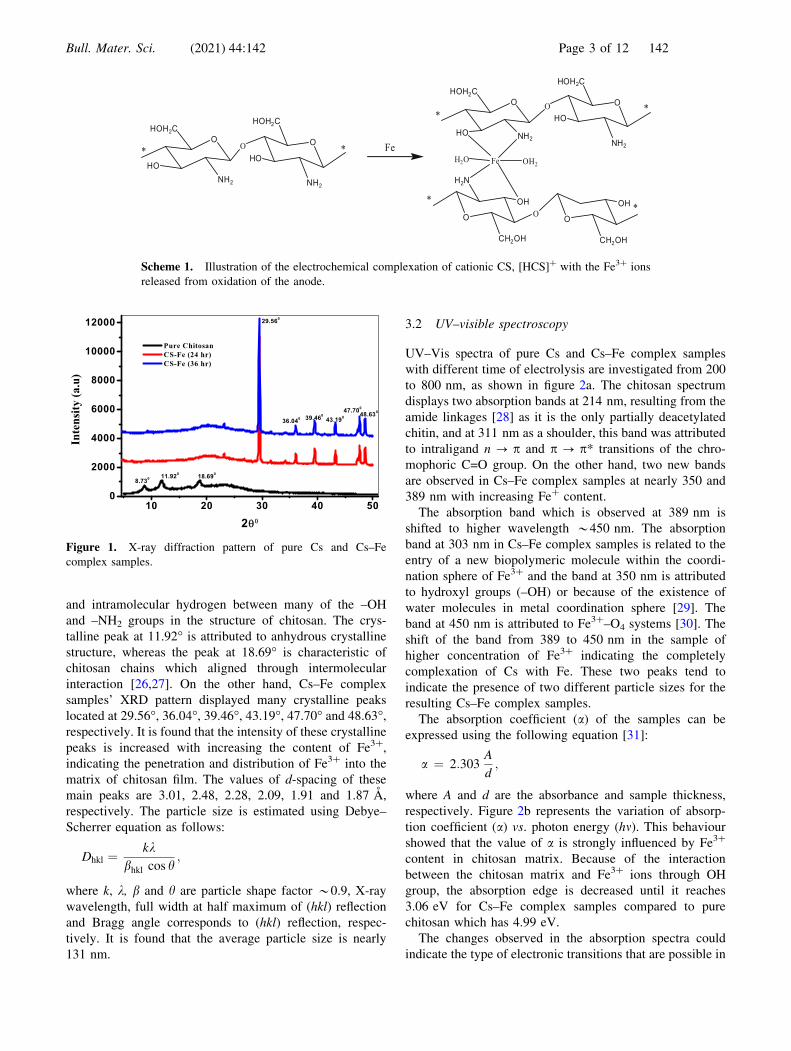
Figure 1 displays XRD pattern of pure Cs and Cs–Fe
complex samples. XRD pattern of pure Cs showed distinct
crystalline peaks at around 2h values at 8.73�, 11.92� and
18.69�. The high degree of crystallization of pure chitosan
is possibly due to the presence of intermolecular
142 Page 2 of 12 Bull. Mater. Sci. (2021) 44:142
and intramolecular hydrogen between many of the –OH
and –NH2 groups in the structure of chitosan. The crys-
talline peak at 11.92� is attributed to anhydrous crystalline
structure, whereas the peak at 18.69� is characteristic of
chitosan chains which aligned through intermolecular
interaction [26,27]. On the other hand, Cs–Fe complex
samples’ XRD pattern displayed many crystalline peaks
located at 29.56�, 36.04�, 39.46�, 43.19�, 47.70� and 48.63�,respectively. It is found that the intensity of these crystalline
peaks is increased with increasing the content of Fe3?,
indicating the penetration and distribution of Fe3? into the
matrix of chitosan film. The values of d-spacing of these
main peaks are 3.01, 2.48, 2.28, 2.09, 1.91 and 1.87 A,
respectively. The particle size is estimated using Debye–
Scherrer equation as follows:
Dhkl ¼kk
bhkl cos h;
where k, k, b and h are particle shape factor *0.9, X-ray
wavelength, full width at half maximum of (hkl) reflection
and Bragg angle corresponds to (hkl) reflection, respec-
tively. It is found that the average particle size is nearly
131 nm.
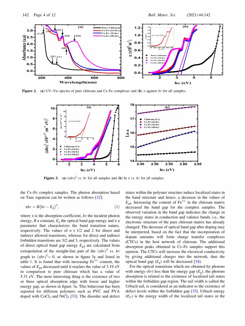
3.2 UV–visible spectroscopy
UV–Vis spectra of pure Cs and Cs–Fe complex samples
with different time of electrolysis are investigated from 200
to 800 nm, as shown in figure 2a. The chitosan spectrum
displays two absorption bands at 214 nm, resulting from the
amide linkages [28] as it is the only partially deacetylated
chitin, and at 311 nm as a shoulder, this band was attributed
to intraligand n ? p and p ? p* transitions of the chro-
mophoric C=O group. On the other hand, two new bands
are observed in Cs–Fe complex samples at nearly 350 and
389 nm with increasing Fe? content.
The absorption band which is observed at 389 nm is
shifted to higher wavelength *450 nm. The absorption
band at 303 nm in Cs–Fe complex samples is related to the
entry of a new biopolymeric molecule within the coordi-
nation sphere of Fe3? and the band at 350 nm is attributed
to hydroxyl groups (–OH) or because of the existence of
water molecules in metal coordination sphere [29]. The
band at 450 nm is attributed to Fe3?–O4 systems [30]. The
shift of the band from 389 to 450 nm in the sample of
higher concentration of Fe3? indicating the completely
complexation of Cs with Fe. These two peaks tend to
indicate the presence of two different particle sizes for the
resulting Cs–Fe complex samples.
The absorption coefficient (a) of the samples can be
expressed using the following equation [31]:
a ¼ 2:303A
d;
where A and d are the absorbance and sample thickness,
respectively. Figure 2b represents the variation of absorp-
tion coefficient (a) vs. photon energy (hm). This behaviour
showed that the value of a is strongly influenced by Fe3?
content in chitosan matrix. Because of the interaction
between the chitosan matrix and Fe3? ions through OH
group, the absorption edge is decreased until it reaches
3.06 eV for Cs–Fe complex samples compared to pure
chitosan which has 4.99 eV.
The changes observed in the absorption spectra could
indicate the type of electronic transitions that are possible in
OHOH2C
NH2
HO
O
HOH2C
NH2
HOO
OHOH2C
NH2HO
O
CH2OH
H2N
OHO
Fe OH2
H2O
Fe
O
HOH2C
NH2
HOO
O
CH2OH
OH
**
**
**
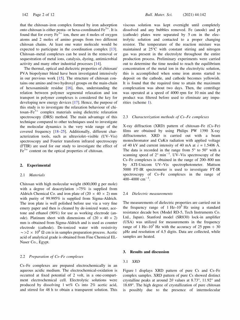
Scheme 1. Illustration of the electrochemical complexation of cationic CS, [HCS]? with the Fe3? ions
released from oxidation of the anode.
10 20 30 40 500
2000
4000
6000
8000
10000
12000
48.63047.700
43.19039.46036.040
29.560
8.730 11.920
Inte
nsity
(a.u
)
Pure Chitosan CS-Fe (24 hr) CS-Fe (36 hr)
18.690
Figure 1. X-ray diffraction pattern of pure Cs and Cs–Fe
complex samples.
Bull. Mater. Sci. (2021) 44:142 Page 3 of 12 142
the Cs–Fe complex samples. The photon absorption based
on Tauc equation can be written as follows [32]:
ahm ¼ B hm� Eg
� �n; ð1Þ
where a is the absorption coefficient, hm the incident photon
energy, B a constant, Eg the optical band gap energy and n a
parameter that characterizes the band transition nature,
respectively. The values of n = 1/2 and 2 for direct and
indirect allowed transitions, whereas for direct and indirect
forbidden transitions are 3/2 and 3, respectively. The values
of direct optical band gap energy Egd are calculated from
extrapolation of the straight-line part of the ahmð Þ2 vs. hm
graph to ahmð Þ2¼ 0, as shown in figure 3a and listed in
table 1. It is found that with increasing Fe3? content, the
values of Egd decreased until it reaches the value of 3.19 eV
in comparison to pure chitosan which has a value of
5.31 eV. The most interesting thing is the existence of two
or three optical absorption edge with lower and higher
energy gap, as shown in figure 3a. This behaviour has been
reported for different polymers such as PVC and PVA
doped with CoCl2 and NiCl2 [33]. The disorder and defect
states within the polymer structure induce localized states in
the band structure and hence, a decrease in the values of
Egd. Increasing the content of Fe3? in the chitosan matrix
decreased the band gap for the complex samples. The
observed variation in the band gap indicates the change in
the energy states in conduction and valence bands, i.e., the
electronic structure of the pure chitosan matrix has already
changed. The decrease of optical band gap after doping may
be interpreted, based on the fact that the incorporation of
dopant amounts will form charge transfer complexes
(CTCs) in the host network of chitosan. The additional
absorption peaks obtained in Cs–Fe samples support this
opinion. The CTCs will increase the electrical conductivity
by giving additional charges into the network, thus the
optical band gap (Eg) will be decreased [34].
For the optical transitions which are obtained by photons
with energy (hm) less than the energy gap (Eg), the photons
absorption is related to the existence of localized tail states
within the forbidden gap region. The tail width is called the
Urbach tail, is considered as an indicator to the existence of
defect levels within the forbidden gap [35]. Urbach energy
(EU) is the energy width of the localized tail states in the
Figure 2. (a) UV–Vis spectra of pure chitosan and Cs–Fe complexes and (b) a against hm for all samples.
Figure 3. (a) (ahm)2 vs. hm for all samples and (b) ln a vs. hm for all samples.
142 Page 4 of 12 Bull. Mater. Sci. (2021) 44:142
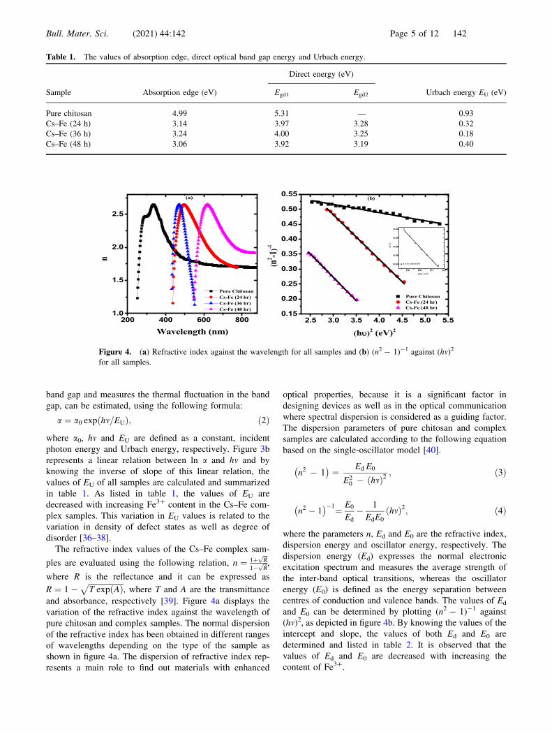
band gap and measures the thermal fluctuation in the band
gap, can be estimated, using the following formula:
a ¼ a0 exp hm=EUð Þ; ð2Þ
where a0, hm and EU are defined as a constant, incident
photon energy and Urbach energy, respectively. Figure 3b
represents a linear relation between ln a and hm and by
knowing the inverse of slope of this linear relation, the
values of EU of all samples are calculated and summarized
in table 1. As listed in table 1, the values of EU are
decreased with increasing Fe3? content in the Cs–Fe com-
plex samples. This variation in EU values is related to the
variation in density of defect states as well as degree of
disorder [36–38].
The refractive index values of the Cs–Fe complex sam-
ples are evaluated using the following relation, n ¼ 1þffiffiffiR
p
1�ffiffiffiR
p ,
where R is the reflectance and it can be expressed as
R ¼ 1 �ffiffiffiffiffiffiffiffiffiffiffiffiffiffiffiffiffiffiT exp Að Þ
p, where T and A are the transmittance
and absorbance, respectively [39]. Figure 4a displays the
variation of the refractive index against the wavelength of
pure chitosan and complex samples. The normal dispersion
of the refractive index has been obtained in different ranges
of wavelengths depending on the type of the sample as
shown in figure 4a. The dispersion of refractive index rep-
resents a main role to find out materials with enhanced
optical properties, because it is a significant factor in
designing devices as well as in the optical communication
where spectral dispersion is considered as a guiding factor.
The dispersion parameters of pure chitosan and complex
samples are calculated according to the following equation
based on the single-oscillator model [40].
n2 � 1� �
¼ Ed E0
E20 � ðhmÞ2
; ð3Þ
n2 � 1� ��1¼ E0
Ed
� 1
EdE0
hmð Þ2; ð4Þ
where the parameters n, Ed and E0 are the refractive index,
dispersion energy and oscillator energy, respectively. The
dispersion energy (Ed) expresses the normal electronic
excitation spectrum and measures the average strength of
the inter-band optical transitions, whereas the oscillator
energy (E0) is defined as the energy separation between
centres of conduction and valence bands. The values of Ed
and E0 can be determined by plotting (n2 - 1)-1 against
(hm)2, as depicted in figure 4b. By knowing the values of the
intercept and slope, the values of both Ed and E0 are
determined and listed in table 2. It is observed that the
values of Ed and E0 are decreased with increasing the
content of Fe3?.
Table 1. The values of absorption edge, direct optical band gap energy and Urbach energy.
Sample Absorption edge (eV)
Direct energy (eV)
Urbach energy EU (eV)Egd1 Egd2
Pure chitosan 4.99 5.31 — 0.93
Cs–Fe (24 h) 3.14 3.97 3.28 0.32
Cs–Fe (36 h) 3.24 4.00 3.25 0.18
Cs–Fe (48 h) 3.06 3.92 3.19 0.40
200 400 600 8001.0
1.5
2.0
2.5
2.5 3.0 3.5 4.0 4.5 5.0 5.50.15
0.20
0.25
0.30
0.35
0.40
0.45
0.50
0.55
5.9 6.0 6.1 6.2
0.24
0.26
0.28
0.30
0.32
n
Wavelength (nm)
Pure Chitosan Cs-Fe (24 hr) Cs-Fe (36 hr) Cs-Fe (48 hr)
(a)
Pure Chitosan Cs-Fe (24 hr) Cs-Fe (48 hr)
(n2 -1
)-1
(h )2 (eV)2
(b)
Cs-Fe (36 hr)35
(n2 -1
)-1
(hu)2 (eV)2
Figure 4. (a) Refractive index against the wavelength for all samples and (b) (n2 - 1)-1 against (hm)2
for all samples.
Bull. Mater. Sci. (2021) 44:142 Page 5 of 12 142

The static refractive index (n0) and static dielectric con-
stant (es) are evaluated by knowing the values of both Ed
and E0 according to the following equation [41]:
n20 ¼ 1 þ Ed
E0
;
es ¼ n20: ð5Þ
The relation between refractive index (n) and wavelength
(k) can be expressed as follows [42]:
n2 ¼ eL � e2
pc2
N
m�
� �k2; ð6Þ
where eL, e, c and (N/m*) are the lattice dielectric constant,
electronic charge, speed of light and carrier concentration to
effective mass ratio, respectively.
The variation of n2 against k2 for all samples is shown in
figure 5. The values of (eL) and (N/m*) are estimated by
knowing the intercept and slope of figure 5 and listed in
table 2. The difference between static and lattice dielectric
constants values can be related to the contribution of free
carriers in the different samples. The values of plasma
frequency of pure chitosan and Cs–Fe complex samples are
calculated using the following equation and listed in table 2
[40].
x2p ¼ e2
e0
N
m�
� �: ð7Þ
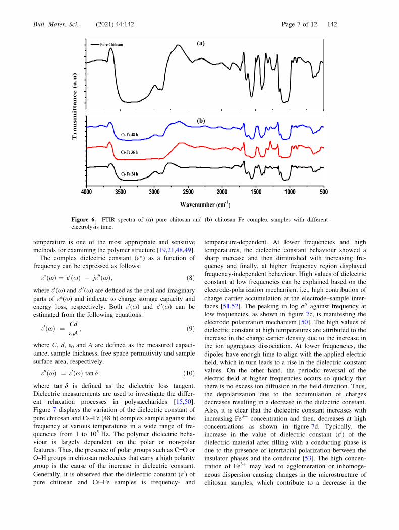
3.3 FTIR spectroscopy
FTIR measurements are more significant tool used to identify
and prove the interactions between Cs molecules and Fe ions
during the electrochemical process and it is considered as an
evidence for the chelation between O and N atoms. FTIR
spectra of Cs–Fe samples with different electrolysis time in
comparison with pure Cs are shown in figure 6. The strong
broad band of pure Cs in the region of 3500–3100 cm-1 is
characteristic of the stretching vibration of O–H and N–H
groups [25]. The characteristic weaker bands at 2932 and
2882 cm-1 are assigned to stretching vibration of aliphatic
C–H bonds of chitosan. The characteristic transmittance
bands at 1640 and 1557 cm-1 are attributed to stretching
vibrations of C=O bond (amide I) and N–H deformation
(amide II) overlapped with NH2, respectively. Transmittance
bands at 1410 and 1383 cm-1 are attributed to bending
vibrations of –OH and –CH3 of the acetyl group, respec-
tively. The bands at 1153 and 1061 cm-1 are assigned to
glycosidic linkages and C–O–C glucose ring vibrations [43].
The band at 1077 cm-1 is attributed to C–O group indicating
that the –COOH group is existed. On the other hand, FTIR
spectra of Cs–Fe samples as shown in figure 6b showed that
the broad band in the region of 3500–3100 is characterized
by a significant decrease in transmittance and more broad-
ness indicating that the N–H vibration is affected due to Fe3?
[44]. Also, the decreasing of band intensity at 1728 cm-1
(stretching vibration C=O, carbonyl group), indicating that
hydrogen bonding reaction within the acetamido group is
broken down in presence of Fe3? [45]. The change in the
transmittance bands around the band 1150 cm-1 reflects to
changes in the secondary carbon hydroxyl group. The
apparent decrease in intensity, as well as shift in position for
1410 and 1383 cm-1 may be attributed to the formation of
complex between chitosan and Fe3? [46]. The metal–ligand
transmission band is observed at 585 cm-1 and assigned to
stretching Fe–N equatorial and the other short transmittance
bands in the region from 800 to 500 cm-1 are assigned due
to the presence of metal–oxygen (Fe–O) [12,47].
3.4 Dielectric spectroscopy analysis
3.4a Dielectric constant: The study of the dielectric con-
stant and dielectric loss as a function of frequency as well as
Table 2. The values of dispersion energy, single oscillator energy, es, eL, N/m* and plasma frequency.
Sample
Dispersion energy,
Ed (eV)
Single oscillator energy,
E0 (eV) es eL
N/m*
(m-3 kg-1)
Plasma frequency
xp (Hz)
Pure chitosan 8.07 4.76 2.69 12.22 5.66 9 1053 4.04 9 1013
Cs–Fe (24 h) 2.71 2.49 2.09 13.15 2.99 9 1053 2.94 9 1013
Cs–Fe (36 h) 1.31 2.63 1.50 26.28 1.03 9 1054 5.46 9 1013
Cs–Fe (48 h) 2.99 2.18 2.37 14.80 2.44 9 1053 2.65 9 1013
1 2 3 4 54
5
6
7
Pure Chitosan Cs-Fe (24 hr) Cs-Fe (36 hr) Cs-Fe (48 hr)
n2
2 (x10-13) m2
Figure 5. n2 against k2 for pure chitosan and complex samples.
142 Page 6 of 12 Bull. Mater. Sci. (2021) 44:142
temperature is one of the most appropriate and sensitive
methods for examining the polymer structure [19,21,48,49].
The complex dielectric constant (e*) as a function of
frequency can be expressed as follows:
e�ðxÞ ¼ e0ðxÞ � je00ðxÞ; ð8Þ
where e0(x) and e00(x) are defined as the real and imaginary
parts of e*(x) and indicate to charge storage capacity and
energy loss, respectively. Both e0(x) and e00(x) can be
estimated from the following equations:
e0ðxÞ ¼ Cd
e0A; ð9Þ
where C, d, e0 and A are defined as the measured capaci-
tance, sample thickness, free space permittivity and sample
surface area, respectively.
e00ðxÞ ¼ e0ðxÞ tan d ; ð10Þ
where tan d is defined as the dielectric loss tangent.
Dielectric measurements are used to investigate the differ-
ent relaxation processes in polysaccharides [15,50].
Figure 7 displays the variation of the dielectric constant of
pure chitosan and Cs–Fe (48 h) complex sample against the
frequency at various temperatures in a wide range of fre-
quencies from 1 to 105 Hz. The polymer dielectric beha-
viour is largely dependent on the polar or non-polar
features. Thus, the presence of polar groups such as C=O or
O–H groups in chitosan molecules that carry a high polarity
group is the cause of the increase in dielectric constant.
Generally, it is observed that the dielectric constant (e0) of
pure chitosan and Cs–Fe samples is frequency- and
temperature-dependent. At lower frequencies and high
temperatures, the dielectric constant behaviour showed a
sharp increase and then diminished with increasing fre-
quency and finally, at higher frequency region displayed
frequency-independent behaviour. High values of dielectric
constant at low frequencies can be explained based on the
electrode-polarization mechanism, i.e., high contribution of
charge carrier accumulation at the electrode–sample inter-
faces [51,52]. The peaking in log r00 against frequency at
low frequencies, as shown in figure 7c, is manifesting the
electrode polarization mechanism [50]. The high values of
dielectric constant at high temperatures are attributed to the
increase in the charge carrier density due to the increase in
the ion aggregates dissociation. At lower frequencies, the
dipoles have enough time to align with the applied electric
field, which in turn leads to a rise in the dielectric constant
values. On the other hand, the periodic reversal of the
electric field at higher frequencies occurs so quickly that
there is no excess ion diffusion in the field direction. Thus,
the depolarization due to the accumulation of charges
decreases resulting in a decrease in the dielectric constant.
Also, it is clear that the dielectric constant increases with
increasing Fe3? concentration and then, decreases at high
concentrations as shown in figure 7d. Typically, the
increase in the value of dielectric constant (e0) of the
dielectric material after filling with a conducting phase is
due to the presence of interfacial polarization between the
insulator phases and the conductor [53]. The high concen-
tration of Fe3? may lead to agglomeration or inhomoge-
neous dispersion causing changes in the microstructure of
chitosan samples, which contribute to a decrease in the
4000 3500 3000 2500 2000 1500 1000 500
Pure Chitosan (a)
(b)
Cs-Fe 48 h
Cs-Fe 36 h
Cs-Fe 24 h
Tra
nsm
itta
nce
(a.u
)
Wavenumber (cm-1)
Figure 6. FTIR spectra of (a) pure chitosan and (b) chitosan–Fe complex samples with different
electrolysis time.
Bull. Mater. Sci. (2021) 44:142 Page 7 of 12 142
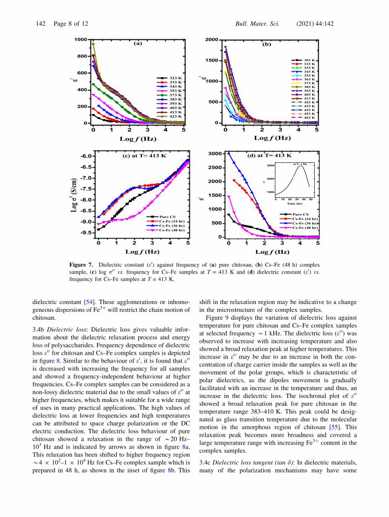
dielectric constant [54]. These agglomerations or inhomo-
geneous dispersions of Fe3? will restrict the chain motion of
chitosan.
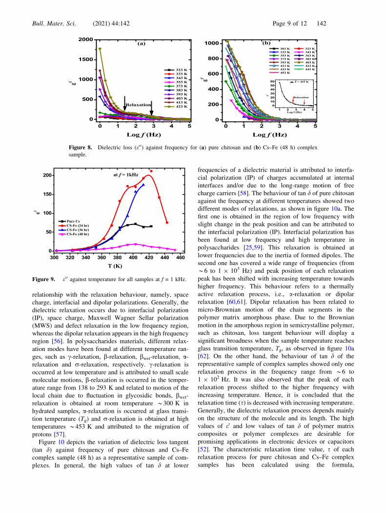
3.4b Dielectric loss: Dielectric loss gives valuable infor-
mation about the dielectric relaxation process and energy
loss of polysaccharides. Frequency dependence of dielectric
loss e00 for chitosan and Cs–Fe complex samples is depicted
in figure 8. Similar to the behaviour of e0, it is found that e00
is decreased with increasing the frequency for all samples
and showed a frequency-independent behaviour at higher
frequencies. Cs–Fe complex samples can be considered as a
non-lossy dielectric material due to the small values of e00 at
higher frequencies, which makes it suitable for a wide range
of uses in many practical applications. The high values of
dielectric loss at lower frequencies and high temperatures
can be attributed to space charge polarization or the DC
electric conduction. The dielectric loss behaviour of pure
chitosan showed a relaxation in the range of *20 Hz–
103 Hz and is indicated by arrows as shown in figure 8a.
This relaxation has been shifted to higher frequency region
*4 9 102–1 9 104 Hz for Cs–Fe complex sample which is
prepared in 48 h, as shown in the inset of figure 8b. This
shift in the relaxation region may be indicative to a change
in the microstructure of the complex samples.
Figure 9 displays the variation of dielectric loss against
temperature for pure chitosan and Cs–Fe complex samples
at selected frequency *1 kHz. The dielectric loss (e00) was
observed to increase with increasing temperature and also
showed a broad relaxation peak at higher temperatures. This
increase in e00 may be due to an increase in both the con-
centration of charge carrier inside the samples as well as the
movement of the polar groups, which is characteristic of
polar dielectrics, as the dipoles movement is gradually
facilitated with an increase in the temperature and thus, an
increase in the dielectric loss. The isochronal plot of e00
showed a broad relaxation peak for pure chitosan in the
temperature range 383–410 K. This peak could be desig-
nated as glass transition temperature due to the molecular
motion in the amorphous region of chitosan [55]. This
relaxation peak becomes more broadness and covered a
large temperature range with increasing Fe3? content in the
complex samples.
3.4c Dielectric loss tangent (tan d): In dielectric materials,
many of the polarization mechanisms may have some
Figure 7. Dielectric constant (e0) against frequency of (a) pure chitosan, (b) Cs–Fe (48 h) complex
sample, (c) log r0 0 vs. frequency for Cs–Fe samples at T = 413 K and (d) dielectric constant (e0) vs.frequency for Cs–Fe samples at T = 413 K.
142 Page 8 of 12 Bull. Mater. Sci. (2021) 44:142
relationship with the relaxation behaviour, namely, space
charge, interfacial and dipolar polarizations. Generally, the
dielectric relaxation occurs due to interfacial polarization
(IP), space charge, Maxwell Wagner Sellar polarization
(MWS) and defect relaxation in the low frequency region,
whereas the dipolar relaxation appears in the high frequency
region [56]. In polysaccharides materials, different relax-
ation modes have been found at different temperature ran-
ges, such as c-relaxation, b-relaxation, bwet-relaxation, a-
relaxation and r-relaxation, respectively. c-relaxation is
occurred at low temperature and is attributed to small scale
molecular motions, b-relaxation is occurred in the temper-
ature range from 138 to 293 K and related to motion of the
local chain due to fluctuation in glycosidic bonds, bwet-
relaxation is obtained at room temperature *300 K in
hydrated samples, a-relaxation is occurred at glass transi-
tion temperature (Tg) and r-relaxation is obtained at high
temperatures *453 K and attributed to the migration of
protons [57].
Figure 10 depicts the variation of dielectric loss tangent
(tan d) against frequency of pure chitosan and Cs–Fe
complex sample (48 h) as a representative sample of com-
plexes. In general, the high values of tan d at lower
frequencies of a dielectric material is attributed to interfa-
cial polarization (IP) of charges accumulated at internal
interfaces and/or due to the long-range motion of free
charge carriers [58]. The behaviour of tan d of pure chitosan
against the frequency at different temperatures showed two
different modes of relaxations, as shown in figure 10a. The
first one is obtained in the region of low frequency with
slight change in the peak position and can be attributed to
the interfacial polarization (IP). Interfacial polarization has
been found at low frequency and high temperature in
polysaccharides [25,59]. This relaxation is obtained at
lower frequencies due to the inertia of formed dipoles. The
second one has covered a wide range of frequencies (from
*6 to 1 9 103 Hz) and peak position of each relaxation
peak has been shifted with increasing temperature towards
higher frequency. This behaviour refers to a thermally
active relaxation process, i.e., a-relaxation or dipolar
relaxation [60,61]. Dipolar relaxation has been related to
micro-Brownian motion of the chain segments in the
polymer matrix amorphous phase. Due to the Brownian
motion in the amorphous region in semicrystalline polymer,
such as chitosan, loss tangent behaviour will display a
significant broadness when the sample temperature reaches
glass transition temperature, Tg, as observed in figure 10a
[62]. On the other hand, the behaviour of tan d of the
representative sample of complex samples showed only one
relaxation process in the frequency range from *6 to
1 9 102 Hz. It was also observed that the peak of each
relaxation process shifted to the higher frequency with
increasing temperature. Hence, it is concluded that the
relaxation time (s) is decreased with increasing temperature.
Generally, the dielectric relaxation process depends mainly
on the structure of the molecule and its length. The high
values of e0 and low values of tan d of polymer matrix
composites or polymer complexes are desirable for
promising applications in electronic devices or capacitors
[52]. The characteristic relaxation time value, s of each
relaxation process for pure chitosan and Cs–Fe complex
samples has been calculated using the formula,
Figure 8. Dielectric loss (e00) against frequency for (a) pure chitosan and (b) Cs–Fe (48 h) complex
sample.
300 320 340 360 380 400 420 440 4600
50
100
150
200
T (K)
Pure Cs CS-Fe (24 hr) CS-Fe (36 hr) CS-Fe (48 hr)
at f = 1kHz
Figure 9. e0 0 against temperature for all samples at f = 1 kHz.
Bull. Mater. Sci. (2021) 44:142 Page 9 of 12 142

s ¼ 1=2pfmax, where fmax is the frequency of each relax-
ation peak position of figure 11.
The activation energy (Ea) values of the relaxation pro-
cess in all samples have been estimated by plotting the
variation of ln s against 1/T, as shown in figure 11. These
plots are found to be linear indicating that s obeys Arrhe-
nius equation as follows:
s ¼ s0 exp Ea=kBTð Þ; ð11Þ
where the parameters s0, Ea and kB are defined as pre-ex-
ponential factor, activation energy and Boltzmann’s con-
stant, respectively. Values of Ea have been calculated by
knowing the slope of the relation between ln s and 1/T and
listed in table 3. It is found that the activation energy values
are decreased as the concentration of Fe3? increased in the
complex samples.
3.4d Cole–Cole plot: Cole–Cole plot gives valuable
information about the electrical performance of dielec-
trics in the form of semicircles. It is found that Cole–Cole
plot of pure chitosan at different temperatures, consists of
two semicircles, one in the low frequency range with
large diameter at high temperatures and the other is
compressed in the high frequency range. The observed
semicircles with large diameters in the low frequency
region and high temperature confirmed the existence of
electrode polarization and interfacial polarization (IP).
On the other hand, the complex samples of Cs–Fe showed
only one semicircle, as shown in figure 12b, and the
semicircles’ radius decreased with increasing Fe3? con-
tent, as shown in figure 12c, indicating the presence of an
activated conduction mechanism [63,64]. It is found that
the sample Cs–Fe (48 h) has the smallest semicircle
diameter revealing that it has the least resistance for
flowing the charges.
0 1 2 3 4 50.0
0.5
1.0
1.5
2.0
2.5
0 1 2 3 4 50.0
0.5
1.0
1.5
2.0
Tan
Log f (Hz)
303 K323 K333 K343 K353 K363 K373 K383 K393 K403 K413 K423 K433 K
(b) Cs-Fe (48 hr) 323 K 333 K 343 K 353 K 373 K 383 K 393 K 403 K 413 K 423 K
Tan
Log f (Hz)
(a) Pure Chitosan
Figure 10. tan d vs. frequency for (a) pure chitosan and (b) Cs–Fe (48 h) complex sample.
2.4 2.5 2.6 2.7 2.8 2.9 3.0 3.1
-10
-9
-8
-7
-6
-5
-4
-3
Pure Chitosan
Cs-Fe (24 hr)
Cs-Fe (36 hr)
Cs-Fe (48 hr)
1000/T (K-1)
Figure 11. ln s vs. 1/T for all samples.
Table 3. Values of activation energy (Ea).
No. Sample Ea (eV)
1 Pure chitosan 0.96
2 Cs–Fe (24 h) 0.83
3 Cs–Fe (36 h) 0.75
4 Cs–Fe (48 h) 0.64
142 Page 10 of 12 Bull. Mater. Sci. (2021) 44:142

4. Conclusion
XRD pattern of Cs–Fe complex samples has been investi-
gated in the range from 5� to 50�. It is found that pure
chitosan is characterized by certain crystalline peaks at
8.73�, 11.92� and 18.96�. The high crystallinity of chitosan
is attributed to the presence of intermolecular and
intramolecular hydrogen between many of the –OH and
–NH2 groups. In addition, the crystallinity of Cs–Fe com-
plex samples is increased with increasing the content of
Fe3?. The optical properties of the complex samples are
investigated using UV–Vis and FTIR spectroscopy. UV–Vis
spectroscopy analysis revealed that pure chitosan is char-
acterized by two absorption bands located at 214 and
311 nm, respectively. These bands are attributed to amide
linkages and intraligand n ? p and p ? p* transitions of
the chromophoric C=O group. On the other side, Cs–Fe
complex samples are characterized by two new bands are
positioned at 350 and 389 nm. With increasing Fe3? con-
tent, these new bands are shifted to new positions and
observed at 359 and 450 nm. The absorption band at
450 nm is attributed to Fe3?–O4 systems indicating that the
complete complexation between chitosan and iron has been
occurred. In addition, it is found that the optical parameters
characterizing Cs–Fe samples are significantly affected due
to the Fe3? content. The most interesting thing is the
existence of two or three optical absorption edge with lower
and higher energy gaps. The values of Egd are decreased
until to reach the value of 3.19 eV in comparison to pure
chitosan which has a value of 5.31 eV. FTIR spectra
showed that many of the characteristic bands of chitosan
have been changed in its position and intensity due to the
presence of Fe3?, confirming that the formation of complex
between chitosan and Fe3? has occurred. The investigation
of dielectric properties of pure chitosan and Cs–Fe complex
samples revealed that both dielectric constant (e0) and
dielectric loss (e00) behaviour have been modified due to the
existence of Fe3?. The high values of e0 at low frequency
and high temperatures are attributed to the electrode
polarization and interfacial polarization in Cs–Fe samples.
Dielectric loss tangent (tan d) showed that pure chitosan is
characterized by two different types of relaxation, the first
one is obtained in the low frequency region and named as
interfacial polarization, while the second is obtained in the
high frequency region and named as dipolar relaxation. On
the other hand, Cs–Fe complex samples are characterized
by only one relaxation process. The activation energy val-
ues of relaxation process are found to be Fe3? content-
dependent and decreased from 0.96 to 0.94 eV.
Acknowledgements
One of the authors (T Fahmy) would like to thank Scientific
Research Deanship, Prince Sattam Bin Abdulaziz Univer-
sity, KSA.
References
[1] Kumar M N, Muzzarelli R A A, Muzzarelli C, Sashiwa H
and Domb A J 2004 Chem. Rev. 104 6017
[2] Won W, Feng X and Lawless D 2002 J. Membr. Sci. 209 493
[3] Nunthanid J, Anan M L, Sriamornsak P, Limmatvapirat S,
Puttipipatkhachorn S, Lim L Y et al 2004 J. Control. Release99 15
[4] Puttipipatkhachorn S, Nunthanid J, Yamamoto K and Peck
G E 2001 J. Control. Release 75 143
[5] Crini G 2006 Bioresour. Technol. 97 1061
[6] Fries C A, Ayalew Y, Barwell J G P, Porter K, Jeffery S L
and Midwinter M J 2014 Injury 45 1111
[7] Shao J, Wang B, Li J, Jansen J A, Walboomers X F and Yang
F 2019 Mater. Sci. Eng. C 98 1053
[8] Das M, Chiellini F, Ottenbrite R M and Chiellini E 2011
Prog. Polym. Sci. 36 981
[9] Wang J and Zhao K 2012 Colloids Surf. A: Physicochem.Eng. Asp. 396 270
Figure 12. Cole–Cole plot of (a) pure chitosan, (b) Cs–Fe (48 h) complex sample and (c) for all samples at T = 413 K.
Bull. Mater. Sci. (2021) 44:142 Page 11 of 12 142

[10] Guibal E 2004 Purif. Technol. 38 43
[11] Domard A 1987 Int. J. Biol. Macromol. 9 333
[12] Rashid S, Shen C, Yang J, Liu J and Li J 2018 J. Environ.Sci. 66 301
[13] Bhatia S C and Ravi N 2000 Biomacromolecules 1 413
[14] Burke A, Yilmaz E, Hasirci N and Yilmaz O 2002 J. Appl.Polym. Sci. 84 1185
[15] Fahmy T, Elhendawi H, Elsharkawy W B and Reicha F M
2020 Bull. Mater. Sci. 43 1
[16] Wang X, Du Y, Fan L, Liu H and Hu Y 2005 Polym. Bull. 55105
[17] Zawodzinski T A, Derouin C, Radzinski S, Sherman R J,
Smith V T, Springer T E et al 1993 J. Electrochem. Soc. 1401041
[18] Natesan B, Karan N K and Katiyar R S 2006 Phys. Rev. E 74042801
[19] Chybczynska K, Markiewicz E, Zasadzinska A G and Bor-
ysiak S 2019 Ceram. Int. 45 9468
[20] Fahmy T, Ahmed M T, El-Kotp A, Abdelwahed H G and
Alshaeer M Y 2016 Inter. J. Phys. Appl. 8 1
[21] Shukur M F, Majid N A, Ithnin R and Kadir M F Z 2013
Phys. Scr. T157 014051
[22] Fahmy T, Ahmed M T, Sarhan A, Abdelwahed H G and
Alshaaer M Y 2016 Inter. J. Appl. Eng. Res. 11 9279
[23] Migahed M D, Ishra M, Fahmy T and Barakat A 2004 J.Phys. Chem. Solids 65 1121
[24] Fahmy T and Ahmed M T 2011 J. Korean Phys. Soc. 581654
[25] Ali A, Elmahdy M M, Sarhan A, Abdel Hamid M I and
Ahmed M T 2018 Polym. Int. 67 1615
[26] Wang S, Shen L, Zhang W and Tong Y 2005 Biomacro-molecules 6 3067
[27] Yamaguchi I, Tokuchi K, Fukuzaki H, Koyama Y, Takakuda
K, Monma H et al 2001 J. Biomed. Mater. Res. 55 20
[28] Hernandez R B, Yala O R and Merce A L R 2007 J. Braz.Chem. Soc. 18 1388
[29] Hernandez R B, Franco A P, Yola O R, Delgado A L, Fel-
cman J, Recio M A L et al 2008 J. Mol. Struct. 877 89
[30] Lever A B P 1984 Inorganic electronic spectroscopy (The
Netherlands: Elsevier)
[31] Ballato J, Foulger S and Smith D W 2003 J. Opt. Soc. Am. B20 1838
[32] Tauc J, Menth A and Wood D 1970 Phys. Rev. Lett. 25 749
[33] Alia H E and Khairy Y 2019 Physica B: Condens. Matter570 41
[34] Devi C U, Sharma A K and Rao V V R N 2002 Mater. Lett.56 167
[35] Urbach F 1953 Phys. Rev. 92 1324
[36] Matin R and Bhuiyan A H 2013 Thin Solid Films 534 100
[37] Fahmy T, Sarhan A, Elsayed I A and Ahmed M T 2018 J.Adv. Phys. 14 5378
[38] Fahmy T, Sarhan A and Elqahtani Z M 2020 Int. J. Eng. Res.Technol. 13 454
[39] Wemple S H and DiDomenico Jr M 1971 Phys. Rev. B 31338
[40] Wemple S H 1973 Phys. Rev. B 7 3767
[41] Pankove I J 1971 Optical processes in semiconductors (NY,
USA: Prentice Hall)
[42] Balevaa M, Goranova E, Darakchieva V, Kossionides S,
Kokkosis M and Jordanov P 2003 Vacuum 69 425
[43] Cui Z, Xiang Y, Si J, Yang M, Zhang Q and Zhang T 2008
Carbohydr. Polym. 73 111
[44] Jin L and Bai R 2002 Langmuir 18 9765
[45] Sipos P, Berkesi O, Tombacz E, Pierre T G and Webb J 2003
J. Inorg. Biochem. 95 55
[46] Rajiv P, Bavadharani B, Kumar M N and Vanathi P 2017
Biocatal. Agric. Biotechnol. 12 45
[47] Fahmy T 2001 Inter. J. Polym. Mater. 50 109
[48] Li Y Q, Zhang C X, Jia P, Zhang Y, Lin L, Yan Z B et al2018 J. Materiomics 4 35
[49] Trivino D G Z, Prokhorov E, Barcenas G L, Nonell J M,
Campos J B G, Pena E E et al 2015 Mater. Chem. Phys. 155252
[50] Fahmy T and Ahmed M T 2003 J. Polym. Mater. 20 367
[51] Furukawa T, Imura M and Yuruzume H 1997 Jpn. J. Appl.Phys. 36 1119
[52] Dang Z M, Yuan J-K, Zha J-W, Zhou T, Li S-T and Hu G-H
2012 Prog. Mater. Sci. 57 660
[53] Saravanan A and Ramasamy R P 2016 J. Polym. Res. 23 104
[54] Campos J B G, Prokhorov E, Barcenas G L, Sanchez I C and
Kovalenko Y 2009 Macromol. Symp. 283–284 199
[55] Zhang T-F, Tang X-G, Liu Q-X, Lu S-G, Jiang Y-P, Huang
X-X et al 2014 Ceram. AIP Adv. 4 107141
[56] Campos J B G, Prokhorov E, Barcenas G L, Garcia A F and
Sanchez I C 2009 J. Polym. Sci. Part B: Polym. Phys. 472259
[57] Luo S, Yu S, Sun R and Wong C-P 2014 ACS Appl. Mater.Interfaces 6 176
[58] Psarrasa G C, Manolakaki E and Tsangaris G M 2003
Composites: Part A 34 1187
[59] Fahmy T and Elzanaty H 2019 Bull. Mater. Sci. 42 220
[60] Fahmy T 2007 Poylm.-Plast. Technol. Eng. 46 7
[61] Fan L, Dang Z, Wei G, Nan C W and Li M 2003 Mater. Sci.Eng. B 99 340
[62] Sengwa R J 2003 Indian J. Pure Appl. Phys. 41 295
[63] Kumar S, Prajapati G K, Saroj A L and Gupta P N 2019
Physica B: Condens. Matter 554 158
[64] Abutalib M M 2019 Physica B: Condens. Matter 557 108
142 Page 12 of 12 Bull. Mater. Sci. (2021) 44:142
Top Related