


Languages
Pages
Legal

Chapter 4The Fourier Series and
Fourier Transform
Chapter 4The Fourier Series and
Fourier Transform
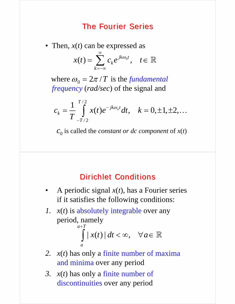
• Let x(t) be a CT periodic signal with period T, i.e.,
• Example: the rectangular pulse trainrectangular pulse train
Fourier Series Representation of Periodic Signals
Fourier Series Representation of Periodic Signals
( ) ( ),x t T x t t R+ = ∀ ∈
• Then, x(t) can be expressed as
where is the fundamental fundamental frequencyfrequency (rad/sec) of the signal and
The Fourier SeriesThe Fourier Series
0( ) ,jk tk
k
x t c e tω∞
=−∞= ∈∑
/ 2
/ 2
1( ) , 0, 1, 2,o
Tjk t
k
T
c x t e dt kT
ω−
−
= = ± ±∫ …
0 2 /Tω π=
is called the constant or dc component of x(t)0c
• A periodic signal x(t), has a Fourier series if it satisfies the following conditions:
1. x(t) is absolutely absolutely integrableintegrable over any period, namely
2. x(t) has only a finite number of maxima finite number of maxima and minima and minima over any period
3. x(t) has only a finite number of finite number of discontinuities discontinuities over any period
Dirichlet ConditionsDirichlet Conditions
| ( ) | ,a T
a
x t dt a+
< ∞ ∀ ∈∫
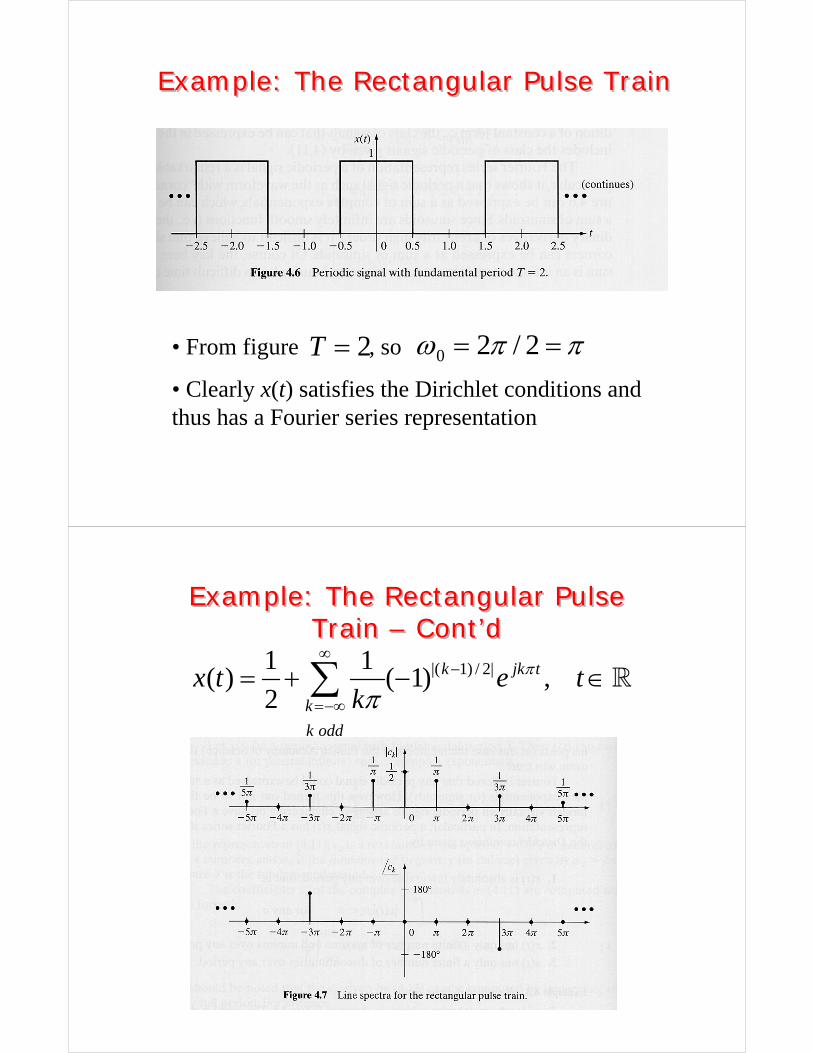
• From figure , so
• Clearly x(t) satisfies the Dirichlet conditions and thus has a Fourier series representation
Example: The Rectangular Pulse TrainExample: The Rectangular Pulse Train
2T = 0 2 / 2ω π π= =
Example: The Rectangular Pulse Train – Cont’d
Example: The Rectangular Pulse Train – Cont’d
|( 1) / 2|1 1( ) ( 1) ,
2k jk t
k
k odd
x t e tk
π
π
∞−
=−∞= + − ∈∑

• By using Euler’s formula, we can rewrite
as
as long as x(t) is real
• This expression is called the trigonometric trigonometric Fourier seriesFourier series of x(t)
Trigonometric Fourier SeriesTrigonometric Fourier Series
0( ) ,jk tk
k
x t c e tω∞
=−∞= ∈∑
0 01
( ) 2 | |cos( ),k kk
x t c c k t c tω∞
== + +∠ ∈∑
dc componentdc component kk--thth harmonicharmonic
• The expression
can be rewritten as
Example: Trigonometric Fourier Series of the Rectangular Pulse Train
Example: Trigonometric Fourier Series of the Rectangular Pulse Train
|( 1) / 2|1 1( ) ( 1) ,
2k jk t
k
k odd
x t e tk
π
π
∞−
=−∞= + − ∈∑
( 1) / 2
1
1 2( ) cos ( 1) 1 ,
2 2k
k
k odd
x t k t tk
πππ
∞−
=
⎛ ⎞⎡ ⎤= + + − − ∈⎜ ⎟⎣ ⎦⎝ ⎠∑

• Given an odd positive integer N, define the N-th partial sum of the previous series
• According to FourierFourier’’s theorems theorem, it should be
Gibbs PhenomenonGibbs Phenomenon
( 1) / 2
1
1 2( ) cos ( 1) 1 ,
2 2
Nk
Nk
k odd
x t k t tk
πππ
−
=
⎛ ⎞⎡ ⎤= + + − − ∈⎜ ⎟⎣ ⎦⎝ ⎠∑
lim | ( ) ( ) | 0NN
x t x t→∞
− =
Gibbs Phenomenon – Cont’dGibbs Phenomenon – Cont’d
3( )x t9 ( )x t

Gibbs Phenomenon – Cont’dGibbs Phenomenon – Cont’d
21( )x t 45 ( )x t
overshootovershoot: about 9 % of the signal magnitude (present even if )N →∞
• Let x(t) be a periodic signal with period T
• The average poweraverage power P of the signal is defined as
• Expressing the signal as
it is also
Parseval’s TheoremParseval’s Theorem
/ 22
/ 2
1( )
T
T
P x t dtT −
= ∫0( ) ,jk t
kk
x t c e tω∞
=−∞= ∈∑
2| |kk
P c∞
=−∞
= ∑

• We have seen that periodic signals can be represented with the Fourier series
• Can aperiodicaperiodic signalssignals be analyzed in terms of frequency components?
• Yes, and the Fourier transform provides the tool for this analysis
• The major difference w.r.t. the line spectra of periodic signals is that the spectra of spectra of aperiodicaperiodic signalssignals are defined for all real values of the frequency variable not just for a discrete set of values
Fourier TransformFourier Transform
ω
Frequency Content of the Rectangular Pulse
Frequency Content of the Rectangular Pulse
( )Tx t
( )x t
( ) lim ( )TT
x t x t→∞
=
• Since is periodic with period T, we can write
Frequency Content of the Rectangular Pulse – Cont’dFrequency Content of the
Rectangular Pulse – Cont’d
( )Tx t
0( ) ,jk tT k
k
x t c e tω∞
=−∞= ∈∑
where
/ 2
/ 2
1( ) , 0, 1, 2,o
Tjk t
k
T
c x t e dt kT
ω−
−
= = ± ±∫ …
• What happens to the frequency components of as ?
• For
• For
Frequency Content of the Rectangular Pulse – Cont’dFrequency Content of the
Rectangular Pulse – Cont’d
( )Tx t T →∞0 :k =
0 1/c T=1, 2, :k = ± ± …
0 0
0
2 1sin sin
2 2k
k kc
k T k
ω ωω π
⎛ ⎞ ⎛ ⎞= =⎜ ⎟ ⎜ ⎟⎝ ⎠ ⎝ ⎠
0 2 /Tω π=

Frequency Content of the Rectangular Pulse – Cont’dFrequency Content of the
Rectangular Pulse – Cont’d
plots of vs. for
| |kT c
0kω ω=2,5,10T =
• It can be easily shown that
where
Frequency Content of the Rectangular Pulse – Cont’dFrequency Content of the
Rectangular Pulse – Cont’d
lim sinc ,2k
TTc
ω ωπ→∞
⎛ ⎞= ∈⎜ ⎟⎝ ⎠
sin( )sinc( )
πλλπλ
sin( )sinc( )
πλλπλ

• The Fourier transform of the rectangular pulse x(t) is defined to be the limit of as , i.e.,
Fourier Transform of the Rectangular Pulse
Fourier Transform of the Rectangular Pulse
( ) lim sinc ,2k
TX Tc
ωω ωπ→∞
⎛ ⎞= = ∈⎜ ⎟⎝ ⎠
kTcT →∞
| ( ) |X ω| ( ) |X ω arg( ( ))X ωarg( ( ))X ω
• Given a signal x(t), its Fourier transform Fourier transform is defined as
• A signal x(t) is said to have a Fourier transform in the ordinary sense if the above integral converges
The Fourier Transform in the General Case
The Fourier Transform in the General Case
( )X ω
( ) ( ) ,j tX x t e dtωω ω∞
−
−∞
= ∈∫
• The integral does converge if1. the signal x(t) is “wellwell--behavedbehaved”2. and x(t) is absolutely absolutely integrableintegrable, namely,
• Note: well behavedwell behaved means that the signal has a finite number of discontinuities, maxima, and minima within any finite time interval
The Fourier Transform in the General Case – Cont’d
The Fourier Transform in the General Case – Cont’d
| ( ) |x t dt∞
−∞
< ∞∫
• Consider the signal • Clearly x(t) does not satisfy the first
requirement since
• Therefore, the constant signal does not have a Fourier transform in the ordinary senseFourier transform in the ordinary sense
• Later on, we’ll see that it has however a Fourier transform in a generalized senseFourier transform in a generalized sense
Example: The DC or Constant SignalExample: The DC or Constant Signal
( ) 1,x t t= ∈
| ( ) |x t dt dt∞ ∞
−∞ −∞
= =∞∫ ∫
• Consider the signal
• Its Fourier transform is given by
Example: The Exponential SignalExample: The Exponential Signal
( ) ( ),btx t e u t b−= ∈
( ) ( )
0 0
( ) ( )
1
bt j t
t
b j t b j t
t
X e u t e dt
e dt eb j
ω
ω ω
ω
ω
∞− −
−∞
=∞∞− + − +
=
=
⎡ ⎤= = − ⎣ ⎦+
∫
∫
• If , does not exist
• If , and does not exist either in the ordinary sense
• If , it is
Example: The Exponential Signal –Cont’d
Example: The Exponential Signal –Cont’d
0b < ( )X ω0b = ( ) ( )x t u t= ( )X ω
0b >1
( )Xb j
ωω
=+
2 2
1| ( ) |X
bω
ω=
+
amplitude spectrumamplitude spectrum
arg( ( )) arctanXb
ωω ⎛ ⎞= − ⎜ ⎟⎝ ⎠
phase spectrumphase spectrum
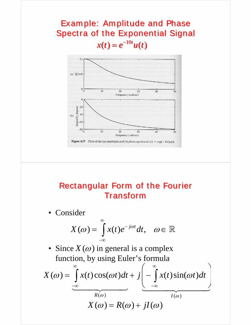
Example: Amplitude and Phase Spectra of the Exponential SignalExample: Amplitude and Phase
Spectra of the Exponential Signal10( ) ( )tx t e u t−= 10( ) ( )tx t e u t−=
• Consider
• Since in general is a complex function, by using Euler’s formula
Rectangular Form of the Fourier Transform
Rectangular Form of the Fourier Transform
( ) ( ) ,j tX x t e dtωω ω∞
−
−∞
= ∈∫( )X ω
( ) ( )
( ) ( )cos( ) ( )sin( )
R I
X x t t dt j x t t dt
ω ω
ω ω ω∞ ∞
−∞ −∞
⎛ ⎞= + −⎜ ⎟
⎝ ⎠∫ ∫
( ) ( ) ( )X R jIω ω ω= +
• can be expressed in a polar form as
where
Polar Form of the Fourier TransformPolar Form of the Fourier Transform
( ) | ( ) | exp( arg( ( )))X X j Xω ω ω=
( ) ( ) ( )X R jIω ω ω= +
2 2| ( ) | ( ) ( )X R Iω ω ω= +
( )arg( ( )) arctan
( )
IX
R
ωωω
⎛ ⎞= ⎜ ⎟
⎝ ⎠
• If x(t) is real-valued, it is
• Moreover
whence
Fourier Transform of Real-Valued SignalsFourier Transform of Real-Valued Signals
( ) ( )X Xω ω∗− =
( ) | ( ) | exp( arg( ( )))X X j Xω ω ω∗ = −
| ( ) | | ( ) | and
arg( ( )) arg( ( ))
X X
X X
ω ωω ω
− =− = −
HermitianHermitiansymmetrysymmetry
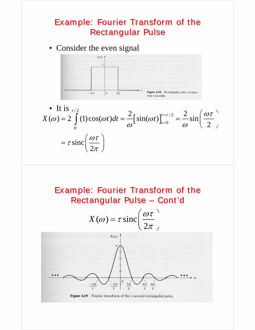
• Consider the even signal
• It is
Example: Fourier Transform of the Rectangular Pulse
Example: Fourier Transform of the Rectangular Pulse
[ ]/ 2
/ 2
00
2 2( ) 2 (1)cos( ) sin( ) sin
2
sinc2
t
tX t dt t
ττ ωτω ω ω
ω ω
ωττπ
=
=
⎛ ⎞= = = ⎜ ⎟⎝ ⎠
⎛ ⎞= ⎜ ⎟⎝ ⎠
∫
Example: Fourier Transform of the Rectangular Pulse – Cont’d
Example: Fourier Transform of the Rectangular Pulse – Cont’d
( ) sinc2
Xωτω τπ
⎛ ⎞= ⎜⎝ ⎠
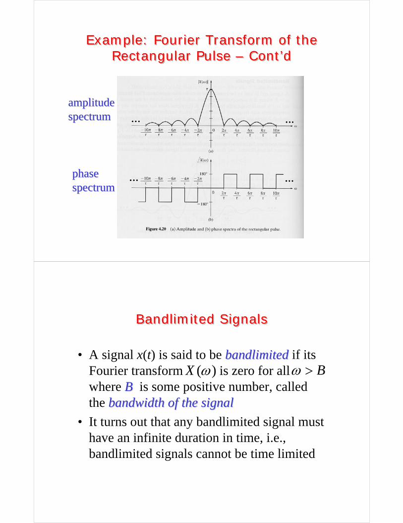
Example: Fourier Transform of the Rectangular Pulse – Cont’d
Example: Fourier Transform of the Rectangular Pulse – Cont’d
amplitude amplitude spectrumspectrum
phase phase spectrumspectrum
• A signal x(t) is said to be bandlimitedbandlimited if its Fourier transform is zero for all where BB is some positive number, called the bandwidth of the signalbandwidth of the signal
• It turns out that any bandlimited signal must have an infinite duration in time, i.e., bandlimited signals cannot be time limited
Bandlimited SignalsBandlimited Signals
( )X ω Bω >

• If a signal x(t) is not bandlimited, it is said to have infinite bandwidthinfinite bandwidth or an infinite infinite spectrumspectrum
• Time-limited signals cannot be bandlimited and thus all time-limited signals have infinite bandwidth
• However, for any well-behaved signal x(t) it can be proven that whence it can be assumed that
Bandlimited Signals – Cont’dBandlimited Signals – Cont’d
lim ( ) 0Xω
ω→∞
=
| ( ) | 0X Bω ω≈ ∀ >B being a convenient large number
• Given a signal x(t) with Fourier transform , x(t) can be recomputed from
by applying the inverse Fourier transforminverse Fourier transformgiven by
•• Transform pairTransform pair
Inverse Fourier TransformInverse Fourier Transform
( )X ω ( )X ω
1( ) ( ) ,
2j tx t X e d tωω ω
π
∞
−∞
= ∈∫
( ) ( )x t X ω↔
Properties of the Fourier Transform Properties of the Fourier Transform
•• Linearity:Linearity:
•• Left or Right Shift in Time:Left or Right Shift in Time:
•• Time Scaling:Time Scaling:
( ) ( )x t X ω↔ ( ) ( )y t Y ω↔
( ) ( ) ( ) ( )x t y t X Yα β α ω β ω+ ↔ +
00( ) ( ) j tx t t X e ωω −− ↔
1( )x at X
a a
ω⎛ ⎞↔ ⎜ ⎟⎝ ⎠
Properties of the Fourier Transform Properties of the Fourier Transform
•• Time Reversal:Time Reversal:
•• Multiplication by a Power of t:Multiplication by a Power of t:
•• Multiplication by a Complex Exponential:Multiplication by a Complex Exponential:
( ) ( )x t X ω− ↔ −
( ) ( ) ( )n
n nn
dt x t j X
dω
ω↔
00( ) ( )j tx t e Xω ω ω↔ −

Properties of the Fourier Transform Properties of the Fourier Transform
•• Multiplication by a Sinusoid (Modulation):Multiplication by a Sinusoid (Modulation):
•• Differentiation in the Time Domain:Differentiation in the Time Domain:
[ ]0 0 0( )sin( ) ( ) ( )2
jx t t X Xω ω ω ω ω↔ + − −
[ ]0 0 0
1( )cos( ) ( ) ( )
2x t t X Xω ω ω ω ω↔ + + −
( ) ( ) ( )n
nn
dx t j X
dtω ω↔
Properties of the Fourier Transform Properties of the Fourier Transform
•• Integration in the Time Domain:Integration in the Time Domain:
•• Convolution in the Time Domain:Convolution in the Time Domain:
•• Multiplication in the Time Domain:Multiplication in the Time Domain:
1( ) ( ) (0) ( )
t
x d X Xj
τ τ ω π δ ωω−∞
↔ +∫
( ) ( ) ( ) ( )x t y t X Yω ω∗ ↔
( ) ( ) ( ) ( )x t y t X Yω ω↔ ∗

Properties of the Fourier Transform Properties of the Fourier Transform
•• ParsevalParseval’’ss Theorem:Theorem:
•• Duality:Duality:
1( ) ( ) ( ) ( )
2x t y t dt X Y dω ω ω
π∗↔∫ ∫
2 21| ( ) | | ( ) |
2x t dt X dω ω
π↔∫ ∫( ) ( )y t x t=if
( ) 2 ( )X t xπ ω↔ −
Properties of the Fourier Transform -Summary
Properties of the Fourier Transform -Summary

Example: LinearityExample: Linearity
4 2( ) ( ) ( )x t p t p t= +
2( ) 4sinc 2sincX
ω ωωπ π
⎛ ⎞ ⎛ ⎞= +⎜ ⎟ ⎜ ⎟⎝ ⎠ ⎝ ⎠
Example: Time ShiftExample: Time Shift
2( ) ( 1)x t p t= −
( ) 2sinc jX e ωωωπ
−⎛ ⎞= ⎜ ⎟⎝ ⎠

Example: Time ScalingExample: Time Scaling
2 ( )p t
2 (2 )p t
2sincωπ
⎛ ⎞⎜ ⎟⎝ ⎠
sinc2
ωπ
⎛ ⎞⎜ ⎟⎝ ⎠
time compression frequency expansion↔time expansion frequency compression↔
1a >0 1a< <
Example: Multiplication in TimeExample: Multiplication in Time
2( ) ( )x t tp t=
2
sin cos sin( ) 2sinc 2 2
d dX j j j
d d
ω ω ω ω ωωω π ω ω ω⎛ ⎞ −⎛ ⎞ ⎛ ⎞= = =⎜ ⎟ ⎜ ⎟⎜ ⎟⎝ ⎠ ⎝ ⎠⎝ ⎠
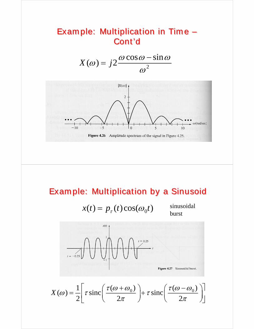
Example: Multiplication in Time –Cont’d
Example: Multiplication in Time –Cont’d
2
cos sin( ) 2X j
ω ω ωωω−
=
Example: Multiplication by a SinusoidExample: Multiplication by a Sinusoid
0( ) ( )cos( )x t p t tτ ω= sinusoidal burst
0 01 ( ) ( )( ) sinc sinc
2 2 2X
τ ω ω τ ω ωω τ τπ π
⎡ ⎤+ −⎛ ⎞ ⎛ ⎞= +⎜ ⎟ ⎜ ⎟⎢ ⎥⎝ ⎠ ⎝ ⎠⎣ ⎦
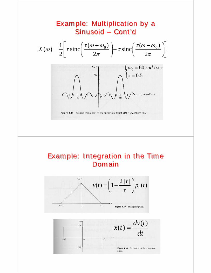
Example: Multiplication by a Sinusoid – Cont’d
Example: Multiplication by a Sinusoid – Cont’d
0 01 ( ) ( )( ) sinc sinc
2 2 2X
τ ω ω τ ω ωω τ τπ π
⎡ ⎤+ −⎛ ⎞ ⎛ ⎞= +⎜ ⎟ ⎜ ⎟⎢ ⎥⎝ ⎠ ⎝ ⎠⎣ ⎦
0 60 / sec
0.5
radωτ
=⎧⎨ =⎩
Example: Integration in the Time Domain
Example: Integration in the Time Domain
2 | |( ) 1 ( )
tv t p tττ
⎛ ⎞= −⎜ ⎟⎝ ⎠
( )( )
dv tx t
dt=
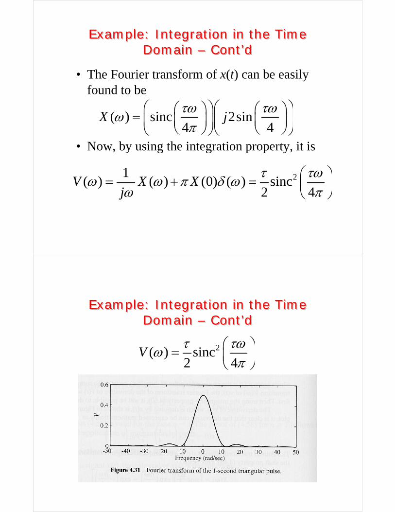
Example: Integration in the Time Domain – Cont’d
Example: Integration in the Time Domain – Cont’d
• The Fourier transform of x(t) can be easily found to be
• Now, by using the integration property, it is
( ) sinc 2sin4 4
X jτω τωωπ
⎛ ⎞⎛ ⎞⎛ ⎞ ⎛ ⎞= ⎜ ⎟ ⎜ ⎟⎜ ⎟⎜ ⎟⎝ ⎠ ⎝ ⎠⎝ ⎠⎝ ⎠
21( ) ( ) (0) ( ) sinc
2 4V X X
j
τ τωω ω π δ ωω π
⎛ ⎞= + = ⎜ ⎟⎝ ⎠
Example: Integration in the Time Domain – Cont’d
Example: Integration in the Time Domain – Cont’d
2( ) sinc2 4
Vτ τωω
π⎛ ⎞= ⎜ ⎟⎝ ⎠

• Fourier transform of
• Applying the duality property
Generalized Fourier TransformGeneralized Fourier Transform
( )tδ
( ) 1j tt e dtωδ − =∫ ( ) 1tδ ↔⇒
( ) 1, 2 ( )x t t πδ ω= ∈ ↔
generalized Fourier transformgeneralized Fourier transformof the constant signal ( ) 1,x t t= ∈
Generalized Fourier Transform of Sinusoidal Signals
Generalized Fourier Transform of Sinusoidal Signals
[ ]0 0 0cos( ) ( ) ( )tω π δ ω ω δ ω ω↔ + + −
[ ]0 0 0sin( ) ( ) ( )t jω π δ ω ω δ ω ω↔ + − −

Fourier Transform of Periodic SignalsFourier Transform of Periodic Signals
• Let x(t) be a periodic signal with period T; as such, it can be represented with its Fourier transform
• Since , it is002 ( )j te ω πδ ω ω↔ −
0( ) jk tk
k
x t c e ω∞
=−∞
= ∑ 0 2 /Tω π=
0( ) 2 ( )kk
X c kω π δ ω ω∞
=−∞
= −∑
• Since
using the integration property, it is
Fourier Transform of the Unit-Step FunctionFourier Transform of
the Unit-Step Function
( ) ( )t
u t dδ τ τ−∞
= ∫
1( ) ( ) ( )
t
u t dj
δ τ τ πδ ωω−∞
= ↔ +∫
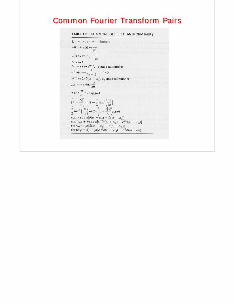
Common Fourier Transform PairsCommon Fourier Transform Pairs
Top Related