


Languages
Pages
Legal


20
CHAPTER 2
REVIEW OF LITERATURE
2.1 GENERAL
Activated Sludge process is the most commonly used treatment
process for treating the domestic / industrial wastewater. Although it is a
proven method of treating wastewater, research on this area still continues to
make the process more effective and successful. The major components
involved in this process are aerator and clarifier. The primary action in the
aerator is the conversion of organic substances into gases that escape to the
atmosphere and into the biological cell tissues that can be removed by gravity
settling in the clarifier. Hence more focus is required in these two processes.
An in-depth study was made as to how these two processes could be made
more effective which prompted the researcher to take up the investigation on
enhancing the biological activity in the aerator and improving the settling
characteristics of activated sludge in the clarifier. To meet the objective of the
above studies, the previous works have been reviewed under the following
related heads.
2.2 DAIRY WASTEWATER TREATMENT
Dairy industry is one of the major industries causing water
pollution. In India, dairy industries generate about 6 – 10 liters of wastewater
per liter of milk processed depending upon the process employed and
products manufactured. Considering the increased milk demand by 2020 AD,

21
the milk based industries in India are expected to grow rapidly and the waste
generation and environmental problems will also increase proportionately.
Poorly treated wastewater with high levels of pollutants caused by poor
design, operation or treatment systems creates major environmental problems
when discharged into surface water or land.
Waste from dairy industries may contain proteins, salts, fatty
substances, lactose and various kinds of cleaning chemicals (Kosseva et al
2003). The treatment of effluent generated from dairy industries, involves
several sequential steps to remove one or more classes of contaminants. The
first step involves primary treatment, where a fraction of the suspended solids
is removed from the wastewater. Following primary treatment, the wastewater
undergoes secondary treatment, which is a biological process, often involving
an aerated lagoon or an activated sludge systems.
In practice, aerated lagoons, as a form of biological treatment, have
often been found inadequate for the new water quality criteria and hence a
more sophisticated process is required. Activated sludge process has been
found superior than other systems in treating the domestic and industrial
wastewater and the plants are capable of reducing BOD and suspended solids
up to 90 to 99 percent, if properly designed and operated.
Fang and Herbert (1990) investigated lab scale aerobic treatment of
dairy wastewater by three stages of activated sludge process. Dairy waste with
an average BOD5 of 1060 mg / L and TKN of 109 mg / L was treated in the
lab scale reactor within the over all retention time of 19.8 h and the final
effluent was found to contain 9 mg / L of BOD5 and 10 mg / L of TKN
corresponding to respective reduction of 99 % and 91%. It was ascertained
that the activated sludge process was an effective way of treating the dairy
wastewater.

22
Orhon et al (1993) investigated experimentally the treatability of
dairy wastewaters by introducing the concept of residual COD. An integrated
dairy plant with small whey production was chosen to evaluate the biological
treatability. Experimental data were interpreted to yield correlations between
removal efficiencies attained with some of the key operation parameters such
as organic loading rate, hydraulic detention time, sludge age etc.
2.3 ACTIVATED SLUDGE PROCESS
2.3.1 Historical Development
The antecedents of the activated sludge process date back to the
early 1880s to the work of scientists who investigated the aeration of
wastewater in tanks and the hastening of the oxidation of the organic matter.
The aeration of wastewater was studied subsequently by a number of
investigators and it was reported that a considerable reduction in putrescibility
could be secured by forcing air into wastewater in basins. Following the
experiments by Clark and Adams (1914) with aerated wastewater, Arden and
Locket in 1914 found that the sludge played an important part in the results
obtained by aeration and named the process as activated sludge process as it
involved the production of an activated mass of micro-organisms capable of
stabilizing organic material in wastewater under aerobic condition (Metcalf
and Eddy 2003).
2.3.2 Biological Reactions in the Aerator
The main function of the aerator is to facilitate aerobic environment
for bioconversion of organic substances into cell tissues with the help of
aerobic bacteria partly inherited from the raw wastewater and partly fed in the
form of activated sludge from the clarifier. The aerobic microbes live and
grow enmeshed in extra cellular polymeric substances that build them into

23
discrete colonies forming three dimensional aggregate microbial structures
called floc.
2.3.3 Microorganisms in the Aerator
When the wastewater is exposed to free oxygen, the aerobic
microorganisms develop on own. Further when the microorganisms are
offered a favorable environment with aeration, required temperature,
appropriate pH and nutrient, they multiply in great numbers. The important
microorganisms that are found in biological treatment process are 1) bacteria
2) fungi 3) algae 4) protozoa 5) rotifers 6) crustaceans and 7) viruses. Among
the above micro organisms bacteria play a major role in converting the
colloidal and dissolved carbonaceous organic matter into various gases and
into cell tissues.
Bacteria are single cell protists. They use soluble food and in
general will be found wherever moisture and food sources are available. Their
usual mode of reproduction is by binary fission, although some species
reproduce sexually or by budding. Even though there are thousands of
different species of bacteria, their general form falls into one of the three
categories. Spherical – sphere shaped (coccus), cylindrical – rod shaped
(bacillus) and helical – spiral shaped (spirillum).
Lilia Mehandjiyska et al (1995) investigated the quantity of
microorganisms in samples of activated sludge from municipal wastewater
treatment during different seasons. It was found that the total number of
microorganisms was greatest during summer and the representatives of genus
pseudomonas predominated in quantitative aspect among the bacteria. While
molds were found during all seasons actinomycetes were isolated only during
summer. The performed investigations gave a possibility of pure cultures to

24
be used for recovering of the distributed ratio of microorganisms in the
activated sludge at extreme situations.
Govoreanu et al (2003) compared the settling properties (SVI) of
the activated sludge with on line measurements of floc size and size
distribution and with microbial community dynamics. Three distinct stages in
the SBR evolution were observed. A good correlation between floc size,
settling properties and microbial community evolution was observed in the
first stage, when the activated sludge was found to have predominant presence
of floc forming bacteria. A good balance between floc-forming and
filamentous bacteria with good settling properties and a highly dynamic
community was observed in the second stage. Finally in the third stage with
an increase in the filamentous bacteria, a good correlation between properties
and floc size distribution was observed.
Rajesh Kumar and Jayachandran (2004) analyzed the treatment of
dairy wastewater using a selected bacterial isolate; Alcaligenes sp. gave a
maximum COD reduction of 90% in 240 hrs. This study clearly indicated the
possibility of using Alcaligenes sp. for the effective treatment of dairy
wastewater.
Maghsoodi Vida et al (2007) examined 10 bacterial isolates from
dairy wastewater for their ability to reduce COD and other chemical
compositions during 30 days. The highest reduction of COD was after
10 days by two micro organisms BP3 (Bacillus with curve) and BP4 (Cocci of
bigger size) and these two were considered as most effective microorganisms
for further experimental performance in order to optimize the efficiency of the
test organisms.
Yan (2007) studied the isolation, characterization and identification
of bacteria from activated sludge and soluble microbial products in
wastewater treatment systems. The standard procedure, medium used,
analytical methods and biochemical characterization techniques required for

25
isolation and identification of bacteria responsible for key process of
wastewater treatment systems were discussed in his study. The effect of
seasonal variations and salinity variations on the bacterial species was also
examined.
Mihaela Palela et al (2008) studied the microbiological and
biochemical characterization of dairy and brewery wastewater micro biota.
The brewery and dairy wastewaters presented a diverse micro biota which
consisted of gram-negative bacteria (the predominant micro-organisms),
yeasts and moulds. The microbiological tests showed the following groups of
microorganisms, such as
Bacteria belonging to the genus bacillus, pseudomonas and
Escherichia.
Yeasts belonging to the genus Saccharomyces, Kluyveromyces
and Torulopisis.
Moulds belonging to the genus Aspergillus and Geotrichum.
Lyliam loperena et al (2009) conducted microbial experiments on
dairy wastewater, isolated the milk fat / protein degrading micro organisms
and developed an inoculum containing pseudomonas sp and bacillas sp. The
bio degradation ability of the inoculum of native organisms was compared
with the ability of commercial inoculum. Although the COD removal was
similar in both cases, the removal of fat and proteins was higher in the case of
native inoculum.
2.3.4 Enzymatic Activity in the Aerator
The enzymes as catalysts have the capacity to increase the speed of
chemical reactions greatly without altering themselves. There are two general
types of enzymes, extracellular and intracellular. When the substrate or

26
nutrient required by the cell is unable to enter the cell wall, the extracellular
enzyme converts the substrate or nutrient to a form that can then be
transported into the cell. Intracellular enzymes are involved in the synthesis
and energy reactions within the cell. There are two physical factors which
have a very pronounced effect on enzyme reactions and they are temperature
and hydrogen ion concentration (pH)
Hisham et al (2004) formulated a dynamic model of the activated
sludge process based on the two kinetic relationships, one with an enzyme –
accelerated reaction associated with non-viable biomass and the other with
monod growth associated with viable biomass. The Michaelis kinetic
relationship represented the enzyme kinetics and Monod kinetics represented
the growth, both using double term definition of substrata uptake and uptake
of DO. The equations were implemented on lab-view, instrumentation –
programming package as virtual instruments and the same were linked to real
instruments and actuators of the plant to function on line.
Yin Li and Chrost (2006) investigated selected enzymatic activities
of microorganisms in three aerobic sludge model reactors of communal, dairy
and petroleum wastewaters. Four extracellular enzymes viz. leucine –
amniopeptidase (L-Amp), - glucocidase ( - GLC), alkaline phosphates
(APA) and lipase (LIP) were studied. Comparison of three wastewater
reactors showed that L-Amp, -GLC and APA had highest activities in dairy
wastewater and the highest activity of LIP was found in petroleum
wastewater. The results of the study showed that the activities of the studied
enzymes were mainly associated with microbial cells in the activated sludge
flocs rather than being cell – free, extra cellular enzymes.. Kinetic parameters
of the studied enzymes varied notably. High Vmax (the maximal hydrolytic
rate) and followed by high Km (michaelis constant) suggested that inhibition
of enzymes took place in the activated sludge system.
27
2.4 REACTIONS IN THE CLARIFIER
The secondary clarifier in activated sludge process has to perform
two functions. 1) Clarification: - Separation of the mixed liquor suspended
solids from the treated waste water, which results in a clarified effluent and 2)
Thickening: Thickening of the return sludge to achieve the desired underflow
concentration of recycling and also to minimize the sludge handling costs.
This is the final step in the products of a well-clarified, stable effluent, low in
BOD and suspended solids. Thus secondary clarifier represents a critical link
in the operation of ASP.
2.5 MICROBIOLOGICAL PROBLEMS IN ASP
Although the conversion of organic wastes into biomass takes place
in the activated sludge process with the help of microorganisms, a few of
them have been found to be creating problems in the system. The types of
microbiological problems that can occur in activated sludge operation include
dispersed (non – settleable) growth, pin floc problems, zoogloeal bulking and
foaming, polysaccharide (Slime) bulking and foaming, nitrification and
denitrification problems, toxicity and filamentous bulking and foaming. The
best approach to trouble shooting the activated sludge process is based on
microscopic examination and oxygen uptake rate (OUR) testing to determine
the basic cause of the problem or upset and whether it is microbiological in
nature.
2.5.1 Filamentous Bulking
Among the various problems that the activated sludge process
encounters, filamentous bulking is one of most common and serious
problems. Bulking is caused by an over abundance of filamentous
microorganisms and termed as filamentous bulking. Eikel boom (1975)

28
provided a rational basis to identify the different filamentous bacteria found in
activated sludge. These filamentous micro organisms grow under different
conditions and there are specific causes for such growth (Table 2.1),(Eikel
Boom 1975).
Paolo Madoni et al (2000) carried out a survey of both biological
bulking and foaming in 167 activated sludge plants and found that 84 had
foaming problem, 81 had bulking problem, and 55 were affected by both the
problems. Bacterial identification reveled that Microthrix parvicella was the
most common filamentous microorganism involved in bulking and foaming.
Other filamentous microorganisms such as Eikel boom types 0041, 021N,
0092, 0675, Thiothrix and Nocardioform Actinomycetes were also reported to
have been detected at lower frequencies. The survey indicated that the use of
contact zone technique or the addition of chemicals such as oxidants and
coagulants were promising approaches for solving bulking and foaming
problems.
Horan et al (2004) assessed the predominant filamentous bacteria
which were found in bulking activated sludge of both domestic origin and
industrial origin in UK. Most samples (84%) of domestic origin were
dominated by two filament types Viz. microthrix parvicella and Eikel boom
type 021N. Remaining 16% of the samples were found to have been
dominated by Nostocoida limicola and sphaerotilus natans. It was reported
that the samples of industrial origin showed much greater filament diversity,
with eight filament types routinely observed in high numbers. Type 021N was
found to be most prevalent and M parvicella was not observed in the
industrial samples. Based upon knowledge of the predominant filament type
from microscopic examination, it was possible to identify the likely causes for
their proliferation and suggest long term solutions to achieve their eradication.

29
Table 2.1 Causes of filament growth in activated sludge
(Eikel Boom D H, 1975).
S.No. Cause Filaments
1Low Dissolved Oxygen
Concentration
Sphaerotilus natans,type 1701
Haliscomenobacter hydrossis
2 Low F/M type 0041,type 0675,type 1851,type 0803
3 Septicity
type 021N,Thiothrix I and II
Nostocoida limicola I,II,III
type 0914,type 0411,type 0961,type 0581
type 0092
4 Grease and OilNocardia spp.,Microthrix parvicella
type 1863
Nutrient Deficiency
Nitrogentype 021N, Thiothrix I and II
5
Phosphorus:
Nostocoida limicola III
Haliscomenobacter hydrossis
Sphaerotilus natans
6 Low pH fungi
Inchio Lou et al (2006) developed new conceptual qualitative frame
work, integrating kinetics and diffusion inside the activated sludge flocs for
explaining filamentous bulking, by operating sequencing batch reactors at
various substrate concentrations and measuring sludge setteleablity at
different floc size distributions. Three different regions (bulking, transitional
and non-bulking region) based on the substrate concentration were suggested.
In the bulking and non-bulking regions, kinetic selection controlled the
growth rate process and favored filaments and floc formers respectively. In
the transitional region, substrate diffusion limitation determined by the floc
size played an important role in causing bulking.

30
2.5.2 Chlorination as a Control Measure for Filamentous Bulking
As discussed in the previous chapter, there are long-term and short-
term methods in controlling the filamentous bulking. The long-term methods
involve the altering the basic parameters of the system which may not be
feasible immediately and involve huge costs. In such cases, the short-term
methods are carried out to control the bulking. Among the short-term
methods, addition of chlorine is commonly practiced, as it is easily available
and cost effective. The most common chlorine compounds used in wastewater
treatment plants are chlorine gas(Cl2), calcium hypochlorite [Ca(OCl)2],
sodium hypochlorite (NaOCl) and chlorine dioxide(ClO2). Chlorine and
hydrogen peroxide have been used successfully to control filamentous
organisms and stop bulking. Chlorine for bulking control is widespread, used
by more than 50% of treatment plants. It should be pointed out that
chlorination is not a cure-all for all activated sludge microbiological
problems. Chlorination will actually make problems worse if the problem is
non-filamentous, e.g., slime bulking or poor floc development (Michael
Richard 1993).
Chlorine dosages for bulking control ranged from 1 to 15 g/kg
MLSS.d according to Jenkins et al (1982) or from 0.7 to 20 mg/L based on
plant sewage throughput rate in seven different activated sludge plants as
reviewed by Neethling (1985a). Neethling et al (1985 a) recommended that
the chlorine dose should not exceed 35 mg/L. Neethling et al (1985b) found
that the filaments associated with low dissolved oxygen concentrations, such
as type 1701 and spherotilus natans, had a lower resistance against
chlorination than the filaments associated with low nutrient levels, such as
Types 0092, 0041, 0675 and M. parvicella. It was found that a chlorine
dosage of 4 g/kg MLSS.d was insufficient to alleviate bulking but a dosage of
double that, was effective, if disruptive to the delicate nutrient removal processes.

31
According to Michael Richard (1993), success was achieved at frequencies as
low as one per day. The recommended dose of chlorine for bulking control
measure is 1 to 10 mg/L. (Metcalf and Eddy 2003).
Neethling et al (1985) developed a model for activated sludge
bulking control by chlorination. The model predicted the frequency of
exposure of chlorine to solids inventory, which related the growth rates of
filamentous and floc forming microorganisms, the proportion and survival
ratios of these two types of organisms. The experimental data of the
laboratory and prototype activated sludge chlorination experiments
substantiated the relation depicted in the model.
Michael Richard (1993) presented the various types of filamentous
organisms that normally cause the bulking and foaming in the activated
sludge and the causative conditions that promote the growth of such
organisms. He also presented the addition of inert material, polymers and
chlorine as methods of choices in controlling the bulking.
Seka et al (2001) investigated the filamentous bacteria causing
bulking in two activated sludge using morphological features, staining
techniques and fluorescent in-situ hybridization. It was identified that the
filaments present in both the sludge were of Eikel boom type 021N. Both the
sludge were tested with the addition of chlorine for control of filamentous
bacteria but it was found that the filamentous bacteria type 021N in one of the
sludge was chlorine susceptible and in other sludge the same type of bacteria
was chlorine resistant. It confirmed the fact that the efficiency of chlorine
depended on penetration rate through the cell wall and suggested that the type
021N bacteria in second sludge developed less permeable cell wall.
Hossain (2004) reviewed the causes of bulking in the activated
sludge process and the control strategies that were normally practiced. The

32
various causes of bulking included low/high DO, low/high organic loading,
reactor configuration, inadequate micro nutrient, low pH, and low relative
influent macro nutrient content. The control measures for activated sludge
bulking could be either system specific and non specific methods. The non
specific methods like addition of polymer, ozone, chlorine etc were employed
as cost effective control strategies, as these methods were cheaper than
modifying plant’s configuration.
2.6 BATCH ANALYSIS OF HINDERED SETTLING
Design of secondary clarifier for biological systems is slightly
different from that of primary clarifier, because of the high solids contents
entering the clarifier from the biological aeration tank. Incoming solids
concentrations are in the range of 2,500 to 5,000 mg/L. Under this situation,
interactions between particles become important and particle settling is
hindered. There is usually a distinct clarified zone showing a liquid-solid
interface. The slope of the hindered settling region is the zone settling
velocity (Vs) that is equivalent to the surface loading rate (Figure 2.1).
Height of
Interface Transition
Compression
t2t1 t3 t4
Zone Settling
Slope Settling Velocity, Vs
Time
Figure 2.1 Interface settling curve
Renko (1998) proposed a model for a batch-settling curve to
determine the solids layers eliminating the disadvantage of the kynch theory
which only offered a graphical procedure for determination. He built the

33
model based on the graphical approach of work and kohler. The applicability
of the model was tested with calcium carbonate solution.
2.7 SETTLING TESTS FOR THE DESIGN OF CLARIFIER
The rate of settling in the hindered settling region is a function of
the concentration of solids and their characteristics. As the settling continues,
a compressed layer of particles forms at the bottom of the cylinder in the
compression settling region. The particles in this region apparently form a
structure in which there is close physical contact between the particles. As the
compression layer forms, regions containing successively lower concentrations of
solids than those in the compression region extend upward in the cylinder.
Thus in actuality, the hindered settling region contains a gradation of solids
concentration from that found at the interface of the settling region to that
found in the compression settling region.
Because of the variability encountered, settling tests are usually
required to determine the settling characteristics of suspensions where
hindered and compression settling are important conditions. On the basis of
data derived from column settling tests, two different design approaches can
be used to obtain the required area of the settling / thickening facilities. In the
first approach, the data derived from a single (batch) settling tests are used. In
the second approach known as the solid flux method, data from a series of
settling tests conducted at different solid concentrations are used.
Jeyanthi and Saseetharan (2006) performed sedimentation experiments
at steady state on dairy activated sludge using columns of different heights
(65,90,120 cms), having a common internal diameter of 2.25 cm for different
MCRT values (5, 7, 9 days) and for various initial MLSS concentrations
(2 g/L to 20 g/L) and determined the zone settling velocities to analyze
the effect of initial height of settling column on biofloc settling. It was

34
determined that there was no appreciable change in zone settling velocity with
respect to height of the settling column and the variation between them was
insignificant.
2.8 SETTLING CHARACTERISTICS
The settling characteristics of the mixed liquor solids must be
considered when designing the secondary clarifier for liquid-solid separation.
Clarifier design must provide adequate area for clarification of the effluent
and thickening of solids for the activated sludge solids. Two commonly used
measures, developed to quantify the settling characteristics of activated sludge
are the sludge volume index (SVI) and the zone settling velocity (ZSV).
2.8.1 Sludge Volume Index
The sludge volume index (SVI) is the % of volume occupied by
1 gm of sludge after 30 minutes of settling. The SVI is determined by placing
a mixed liquor sample in a 1 to 2 L cylinder and measuring the settled volume
after 30 minutes and the MLSS concentration of corresponding sample.
Koopman and Cadee (1983) predicted the thickening capacity,
using diluted sludge volume index. The parameters characterizing functional
relationship between settling velocity and suspended solids concentration
were correlated with an easily measured index of sludge settleability, the
diluted sludge volume index (SVI).
Daigger and Roper (1985) developed graphical methods to estimate
activated sludge settling characteristics which were claimed to be applicable
over a broad range of sludge settleablity. The secondary clarifier design and
performance evaluation could be accomplished for an expected range of SVIs,
given the solids loading rate and the corresponding underflow concentration.

35
Renko (1998) developed a model for describing a relationship
between zone settling velocity and stirred SVI. The model gave a good fit
with large SVI and concentration ranges offering a promising relationship
linking ZSV and stirred sludge volume index. The model had greater
advantages of eliminating tiresome multiple batch settling tests.
Bo Jin et al (2003) presented a comprehensive study of sludge floc
characteristics and their impact on compressibility and settleability of
activated sludge in full scale wastewater treatment processes. Compressibility
and settleability were defined in terms of the sludge volume index and zone
settling velocity. It was observed that the morphological and physical
properties of floc had important influence on the sludge compressibility and
settleability.
2.8.2 Zone Settling Velocity
The secondary clarifier design has also been related to an expected
zone settling velocity (ZSV). The ZSV is the settling velocity of the sludge /
water interface at the beginning of sludge settleability test. Many empirical
relations have been suggested to describe the relation between ZSV and
MLSS concentration. The Vesilind relation (Vesilind 1974) is generally
accepted in describing the Vs – Co relation as it is considered to be very
accurate and simple.
Vs = Vo e(-a Co)
(2.1)
In the above Vesilind equation Vo is the maximum settling velocity
and ‘a’ is the measure on how fast the settling velocity decreases with the
increase in concentration of particles.

36
Daigger (1995) presented an analysis of five sludge settling
characteristics data sets from many suspended growth biological wastewater
treatment processes. The results indicated that the data could be characterized
using a single relationship between the initial sludge settling velocity (Vi), the
initial sludge Concentration (Ci) and the sludge volume index (SVI) by means
of an equation (2.2)
Vi = 1.871 – (0.1646 + 0.0051586 SVI) Ci (2.2)
Christopher and Peter (1998) developed a simple mechanistic
model to evaluate the effects of solid characteristics and test parameters on
SVI type indices. It was inferred that for solids settleability and compatibility,
the settling column height and solids concentration in the test had an
interactive effect on the measured SVI. This modeling approach provided a
method for assessing the relevance of the different techniques as valid
measures of solids settleability and assessing whether it was valid to correlate
ZSV model parameters to SVI type measures.
Christopher and Peter (1999) evaluated various correlations by
comparing predicted parameters of Vo (m / h) and K (m3 / Kg) to true Vo and
K values in the equation (2.3)
Vs = Vo. e–k x
(2.3)
To determine the parameters, several column-settling tests over a
range of solids concentrations were performed. Minimum and maximum SVI
values for each Vo and K pair were identified from the profile. The difference
in maximum allowable over flowrate of settling tank, when flux theory design
was applied based on the true and correlation generated ZSV parameters, was
also assessed.

37
Alexis Vandehasselt and Peter Vanrolleghem (2000) obtained the
parameters for the settling velocity models by two ways. One, the traditional
approach using zone settling velocity data from dilution experiments and
other, the direct estimation method relying on a single batch settling curve.
Both the parameters were compared. Four distinct sludge settling curves were
recorded at different sludge concentrations and the Vesilind parameters were
calculated in the traditional way. The value of the resulting model was
evaluated by cross-validating it, on its ability to describe complete single
batch settling curves. The flux curves associated with the single batch settling
curves were estimated. It was concluded that the reliability of single batch
settling curve based flux curve predictions was insufficient to warrant
replacement of the traditional estimation of settling characteristics.
Richard et al (2001) evaluated the settling characteristics of mixed
liquor from advanced wastewater treatment and conventional wastewater
treatment facilities. An algorithm was developed that related zone settling
velocity (Vs) of the mixed liquor to initial mixed liquor suspended solids
(MLSS) concentration and unstirred sludge volume index (USVI) of the
mixed liquor. A secondary clarifier operating diagram was presented that
could be used in the design and operation of secondary clarifiers.
2.9 DESIGN APPROACHES OF SECONDARY CLARIFIER
There are two methods of design of secondary clarifier.
(i) Talmadge and Fitch method.
(ii) Solid flux method.

38
2.9.1 Talmadge and Fitch Method
A column of height Ho is filled with a suspension of solids of
uniform concentration Co. The position of the interface as time elapsed and
the suspension settled is given as shown in Figure 2.2. The rate at which the
interface subsided is given by the slope of the curve at any point.
The critical concentration controlling the sludge handling capacity
of the tank occurs at a height, Hc where the concentration is Cc (critical
concentration). This point is determined by extending the tangents to the
hindered and compression settling regions of the settling curve to the point of
intersection and bisecting the angle thus formed as shown in Figure 2.2. From
point Cc, a horizontal line is drawn which cuts the ordinate at Hc.
Figure 2.2 Talmadge and Fitch method
From the mass balance Co Ho = Cc Hc,
Cc = Co Ho / Hc,
HO
HC
HU
tU
CC
Time
Inte
rface h
eig
ht
Ho – Initial height
Hu – Height at which underflow concentration is reached
Hc – Height at which critical concentration is reached
Cc – Point of critical sludge concentration
tu – Point of critical sludge concentration
39
where, Ho = height of the column, m
Co = initial concentration of suspension, mg/L
Hc = Critical height, m
Through point Cc , a tangent is drawn. The desired underflow
concentration of sludge from the tank is taken as Cu. Again from mass balance
Co Ho = Hu Cu, the height Hu at which the desired underflow concentration
reached is determined.
Hu = Co Ho/Cu
A horizontal line at depth Hu is constructed. A vertical line from the
point of intersection of the two lines drawn through Cc and Hu to the time axis
is constructed to get the value tu, (i.e.) the time required to reach the desired
under flow concentration Cu. Then the required thickening area is calculated
using the relationship,
Q/A = Ho/tu,
where, Q = Flow m3 / day
A = Surface area of the tank, m2
Ho = Initial column Height, m
tu = Time required to reach the desired under flow concentration
Cu, min
The thickener area, At = Q tu/Ho
The thickener area of settling tank designed based on zone settling,
as above, is checked for adequacy for clarification.
Area required for clarification (Ac) = Q1/ZSV
40
where, Q1 = Q (Ho – Hu)/Ho.
ZSV = Zone Settling Velocity, m/min
Normally the thickener area controls the design.
2.9.2 Solid Flux Analysis
An alternative method of arriving at the area required for hindered
settling has been delineated by Coe and Clevenger (1916), Yoshioka et al
(1957), Keinath et al (1977).
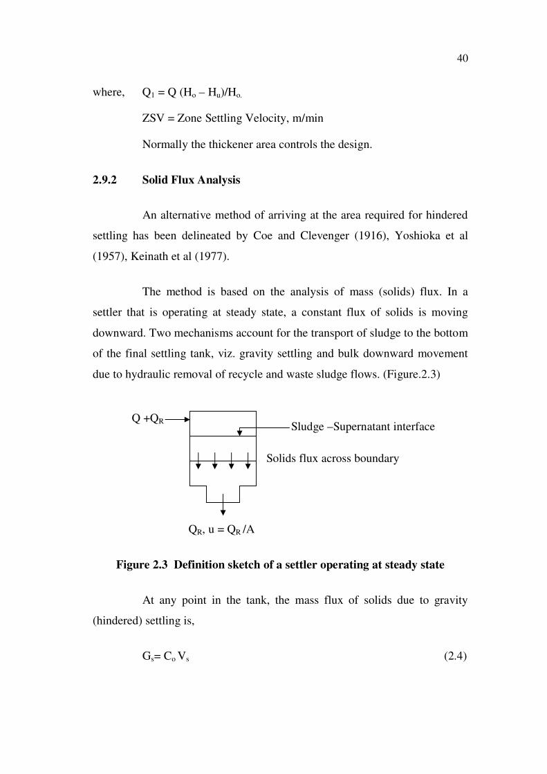
The method is based on the analysis of mass (solids) flux. In a
settler that is operating at steady state, a constant flux of solids is moving
downward. Two mechanisms account for the transport of sludge to the bottom
of the final settling tank, viz. gravity settling and bulk downward movement
due to hydraulic removal of recycle and waste sludge flows. (Figure.2.3)
QR, u = QR /A
Figure 2.3 Definition sketch of a settler operating at steady state
At any point in the tank, the mass flux of solids due to gravity
(hindered) settling is,
Gs= Co Vs (2.4)
Q +QRSludge –Supernatant interface
Solids flux across boundary

41
The settling velocity of the particles should control the design for
this zone. In this zone the solids flux is called the gravity flux.
The mass flux of solids due to the bulk movement of the suspension
(i.e.) due to sludge withdrawal is
Gu = Co u = Co (QR/A) (2.5)
It represents the concentrated sludge zone, where thickening of
sludge occurs. The rate of sludge withdrawal is the controlling factor. In this
zone the solids flux is defined as the underflow flux. The total mass flux is the
sum of previous components and is given by
GT = Gs+ Gu = Co Vs + Co u (2.6)
In a batch test, the downward movement of sludge solids is due to
the settlement velocity. Thus the batch solids flux can be denoted as given in
Eqn 2.4. Also, gravity flux depends on the concentration of solids and the
settling characteristics of the solids at that concentration. The procedure used
to develop a solids flux curve from column settling data is illustrated below.
Hindered settling velocities are derived from column settling test for
suspension at different concentrations. The resulting Velocity-concentration
data pairs can be used to calculate the gravity solids flux. Each value of Gs
represents the gravity solids flux per unit area of the clarifier that would be
expected to occur at the corresponding activated sludge concentration.
At low concentration, (below 1g/L) the movement of solids due to
gravity is small, because the settling velocity of the solids is more or less
independent of concentration. If the velocity remains essentially the same, as
the concentration increases, the total flux due to gravity starts to increase. At
very high solids concentrations, the hindered settling velocity approaches zero

42
and the total solids flux due to gravity again becomes extremely low. Thus it
can be concluded that the solids flux due to gravity must pass through a
maximum value, as concentration is increased. (Figure 2.4(a)) The solids flux
due to bulk transport is a linear function of the concentration, with the slope
equal to u, the underflow velocity. Because the underflow velocity can be
controlled, it is used for process control.
The required cross sectional area for thickening is determined by
drawing a horizontal line tangent to the total flux curve (Figure 2.4(a)). Its
intersection with the vertical axis represents the limiting solids flux GL, which
can be processed in the settling tank. The corresponding underflow
concentration is obtained by dropping a vertical line to X-axis from the
intersection of the horizontal line and the underflow flux line (Metcalf and
Eddy 2003). GL is the maximum allowable flux loading if the settling is to be
successful. If the influent flux to the settler is larger than GL, the sludge
blanket will increase, resulting in solids in the effluent. The limiting flux can
be used for the design of the area of the settler.
Saseetheeran et al (1997) performed zone settling studies on
domestic activated sludge and developed mathematical models for calculating
surface area for secondary settling tank keeping initial suspended solid
concentration of the sludge (Co), recycling ratio(R), desired underflow sludge
concentration (Cu) and mean cell residence time ( c) as process parameters.
The developed models were used for preparing nomograms from which the
area of secondary settling tank could be found graphically for any known
process parameters. The range of a mass concentration to be maintained in the
reactor in-order to obtain the required underflow concentration was also
suggested.
43
Jiri Wanner (2003) analyzed the three functions of secondary
clarifiers Viz.
Solid – liquid separation having direct effect on effluent
quality.
Sludge thickening importance to control the sludge age.
Storage capacity determining the sludge distribution between
biological reactor and settler.
The various flow configurations for both circular and rectangular
settlers and the specific case of a circular secondary settler with radial flow
was analyzed in detail. Range of values for the classical design parameters
like hydraulic loading, hydraulic retention time, solid flux, hydraulic loading
of the effluent weirs, recycle ratio were identified.
Sekaran and Rajagopal (2007) conducted batch settling tests for the
activated sludge of sugar and tannery industries using a cylindrical thickener.
Zone settling velocities and suspended solids concentration were used to
develop logarithmic models. Limiting solids flux was obtained from solid
flux curves that were prepared for both the wastewaters. The solids flux
loading was found to be high for sugar industry wastewater compared to
tannery industry wastewater.
2.9.3 Modified Solids Flux Analysis
An alternative graphical technique of analysis for determining GL,
developed by Yoshioka et al (1957) allows the determination of the limiting
flux simply by drawing a line tangent to the flux curve which intersects the
X- axis at the desired underflow concentration, Cu. (Figure 2.4b). This line
has a negative slope of ‘u’. Similarly a line from the origin to any point on the

44
settling flux curve has a slope of Q/A. The analogy between the total flux
curve and this technique can be observed by inspection. The latter has been
employed because it offers the advantages of simplicity and versatility in
application. This method is especially useful where the effect of the use of
various underflow concentrations on the size of the treatment facilities is to be
evaluated.
C0 CL
Total flux
GL
Soli
d F
lux
K
g/m
².h
r
MLSS Concentration g/LCu
GL
-u
Go
Soli
d F
lux
K
g/m
².h
r
MLSS Concentration g/L
Q/A
A
CuCo
Underflow Flux
Gravity Flux
Limiting Flux
Figure 2.4(a) Solid flux analysis Figure 2.4(b) Modified solid flux analysis
The gravity solid flux for any value of Co is obtained by
multiplying zone settling velocity Vs with its respective initial MLSS
concentration Co. A plot was drawn between GG and Co to obtain the limiting
solids flux (GL) graphically by modified solids flux method of analysis as
shown in Figure 2.5. A tangent drawn to the gravity solids flux curve
originating from the desired value of Cu will yield the value of GL on the
Y- axis. By dropping a vertical line from the point where the tangent touches
the gravity flux curve, the value of maximum MLSS concentration (Cmax) to
be maintained in the reactor is obtained on the X-axis for Cu under
consideration. The equations derived from materials balance for calculating
Co and A/Q for any value of Cu, GL and R are given below.

45
Figure 2.5 Modified solids flux method of analysis
Co = [R / (1+R)] Cu (2.7)
A /Q = [(1+R) Co] / GL = R Cu/GL (2.8)
where, A/Q = Surface area per unit flow rate, m2/m
3/h
GL = Limiting solids flux, Kg/m2.h
R = Recycling ratio, QR /Q
Co = Influent MLSS concentration, g/L
Cu = Desired underflow concentration, g/L
Yunsheng Zheng and David (1998) proposed a model for predicting
the solids concentration profile in the zone settling and compression regimes
of the thickener. The model was based on a function relating effective solids
pressure to solids concentration and the rate of change of solids concentration.
The model was applied to steady state secondary clarifiers and provided good
agreement with literature data for both laboratory and field scale clarifiers.
Total flux
Underflow flux
Limiting flux
Gravity flux
Cu
CLVL
GL =
CLV
L+
CLU
b
Ci CL
CiVi
CiUb
Ub
So
lid
flu
x,
kg
/m2.h
Solids concentration, Kg/m3 (g/L)
CiVi + CiUb
GL

46
Jeyanthi and Saseetharan (2007) performed multiple batch settling
tests on dairy activated sludge at steady state, stationary phase and in
endogenous phase. Mathematical models were developed for the thickener
area of clarifier by correlating process control parameters such as MCRT,
MLSS concentration, underflow concentration and recycling ratio. The flux
curves were utilized in the generation of clarifier operation and control data.
2.10 PROCESS DESIGN PARAMETERS
The clarifier cannot be designed in isolation without considering
the process output of an aerator, as clarifier is an integral part of the ASP.
Hence it is very essential to consider all the parameters that influence the
overall process. Following process loading parameters determine the
efficiency of the activated sludge settling (Martin and James 1999).
2.10.1 F/M Ratio
The food / microorganism ratio, commonly referred to as F/M is
equivalent to the BOD loading rate divided by mass of MLSS in the reactor.
F/M = Q S / V X (2.9)
It is clear from the above equation that the F/M ratio is otherwise a
feeding rate. The lower the F/M ratio, the lower the feeding rate is, the
hungrier the microorganisms and the more efficient the removal will be. At
high F/M ratios, the microorganisms are maintained in the accelerating or
exponential growth phase. These organisms are more food saturated (i.e.)
there is an excess of substrate and thus BOD removal is less efficient.
Common ranges for F/M for a conventional activated sludge plant are from
0.15 to 0.5.

47
2.10.2 Sludge Age
Sludge age is defined as the average time in days that the
suspended solids remain in the entire system.
MLSS in aerator (kg)
Sludge age in days = (2.10)
Primary effluent SS (kg/day)
The common range for sludge age for a conventional activated
sludge plant is between 3 and 15 days.
2.10.3 Growth Rate
In order to evaluate the effect of substrate concentration and other
factors of the microbial activity, it is necessary to study the growth rate of
microorganisms (Benefield and Clifford 1980). The specific growth rate of
microorganisms is given by
x
dtdx
(2.11)
= kg. MLSS produced /kg MLSS present in the reactor per day
increases as substrate concentration increases until it levels off at
the maximum possible valve of given by Monod`s empirical function.
Sk
S
s
max (2.12)
Abdul Kareem (2004) developed a model to predict the values of
the specific growth rate of micro-organisms in the plant and the biomass
concentration, given the substrate utilized and the dilution rate with the

48
wastewater plant of textile industry. In evaluating the model, some kinetic
parameters such as Kd, Y, Ks, M, Ka1 and Ka2 were determined by statistical
analysis of the experimental results. There was a remarkable agreement
between the simulation results and the experimental results.
Stroot et al (2005) used mathematical modelling and quantitative
whole cell 16s rRNA – targeted fluorescence in-situ hybridizations (FISH) to
predict and determined experimentally the in- silico and in-situ net growth
rates of individual microbial populations in activated sludge systems during
start-up to steady state conditions. The results challenged the perception that
the net growth rate of microorganisms in an activated sludge system reached a
“steady state” value after three times the MCRT.
2.10.4 Mean Cell Residence Time / Solids Retention Time
In order to keep the F/M stable, some MLSS must be continuously
wasted to balance this microorganism’s biomass produced through growth.
The design and operation parameter for determining rates of MLSS wastage is
the solids retention time ( c days) defined as the mass of solids present in the
reactor over the mass of solids wasted per unit time.
V X
c days = (2.13)
Qw Xw
= kg MLSS present in reactor / kg MLSS wasted per day
where, Qw is the waste sludge flow from the reactor. Values of c, ranging
from 3 to 15 days result in the production of a stable, high quality effluent
with excellent characteristics. Thus recommended values for c can be used to
calculate the required waste sludge flow. Also

49
1 / c, day-1
= Qw Xw / VX (2.14)
= Kg MLSS wasted / kg MLSS present in the reactor per day.
From the definition of the specific growth rate of microorganisms,
dx / dt
= (2.15)
X
it is seen that MCRT is equal to 1/ . Hence by controlling c, the specific
growth rate and thus the physiological state of the organisms in the system
can be controlled. That is, the control of the process can be exercised simply
by regulating Qw.
Adrien (1998) derived a formula for the mean cell residence time,
considering the total time of microorganisms remained in suspended solids
with the treatment system, from the entry of the cells into the reactor to the
solid separation unit including any channel, where the cell residence time was
significant. It was finally shown that under appropriate assumptions, it was
equivalent to the formula commonly used.
Jenson (2001) explored the validity of the general assumption that
the steady state in a mixed flow reactor approaches at three hydraulic
residence times. For well mixed systems, the time to approach steady state
depends on the kinetic order of removal mechanisms, the initial pollutant
concentration in the control volume and the kinetic rate constant. The
assumption of three hydraulic residence times to steady state was found to be
conservative.

50
2.10.5 Clarifier overflow Rate
As the floc settles in a clarifier, the displaced water rises upward.
The upward velocity of water is termed the over flowrate (OFR) with unit m3
/ day / m2 and is determined by dividing flow (m
3 / d) by the clarifier surface
area m2. When a clarifier is operated at a specified OFR, all particles having
settling velocities higher than the operating OFR will be removed, while
particles with lower settling velocities are carried over the effluent weir. By
selecting a proper OFR, clarification is ensured. The clarifier overflow rate is
independent of recycle flow rate and is expressed as
OFR= QE / A (2.16)
QE = clarifier effluent flow rate [m³/d]
A = clarifier surface area [m²]
Bryan and Keinath (1983) constructed a small pilot scale
completely mixed activated sludge treatment plant and investigated the
functional effects of three parameters Viz. Solids retention time, hydraulic
retention time and clarifier over flowrate on clarification efficiency. It was
concluded that the changes in HRT and SRT together in the same phase
resulted in higher effluent solids and increasing either variable, while
decreasing other resulted in improved quality of the effluent with respect to
suspended solids. Maintaining one variable constant, while varying the other
showed that initial suspended solids concentration was slightly more sensitive
to SRT than HRT.
2.10.6 Solids Loading Rate
Solids loading rate is the mass rate of suspended solids into the
clarifier divided by the tank cross sectional area. The total mass rate is the

51
sum of tank effluent flow rate and RAS flow rate. The solids loading rate to
an activated sludge clarifier should not be the greater than the limiting solids
flux in the clarifier. This parameter is as important as over flowrate, in
determining the capacity of an activated sludge clarifier.
[Q influent + Q RAS] C influent
SLR= ------------------------------------------------------ (2.17)
A clarifier
Youngchul Kim and Wesely (1999) studied the estimation of the
sludge blanket and commented that the method of obtaining the suspended
solids concentration, by averaging the mixed liquor suspended solids and the
return sludge suspended solids concentration, frequently resulted in over
estimated by large amount. Hence an exponential equation was developed by
analysis of data from plant operation and from a special study of sludge
blanket, for various over flow rates and sludge characteristics.
2.10.7 MLSS Concentration
MLSS concentrations in the range of 1500 to 3500 mg / L are often
used. Because the MLSS concentration affects the solids loading on the
secondary clarifier, selection of the MLSS concentration must be coordinated
with the secondary clarifier design.
Kazmi and Furumai (2000) proposed a simple settling model for
the batch activated sludge process, that could predict sludge concentration
profile as a function of time. The model was applied by giving easily measurable
parameters namely, the initial mixed liquor suspended solids concentration,
sludge interface variation and sludge volume index. The model described the
sludge sedimentation process by linking three concentrations.1) MLSS on
sludge interface. 2) Constant MLSS on sediment surface 3) Variable MLSS at the
bottom. The model was tested for wide ranges of activated sludge

52
concentrations (1750 – 4630 mg/L) and SVI (104 – 265). A simulated MLSS
profile linking three critical concentrations agreed well with observation data.
2.10.8 Oxygen Requirement
The oxygen requirement must be adequate to satisfy carbonaceous
BOD of the waste, the endogenous respiration of the biomass, the oxygen
demand for nitrification, adequate mixing and maintain a minimum DO
concentration throughout the aeration tank.
2.10.9 Sludge Recycling Rate or Return Sludge Flow Rate
The recycle rate depends on the settling and thickening
characteristics of the sludge with clarifier and hence it varies. It influences the
design of the clarifier in terms of the size without influencing the size of the
aeration tank. The range is typically from 25 to 100% of the average design
flow, though peak hourly flow needs must be accommodated.
Antonio and Carbone (1987) compared two models of the kinetics
of the biological removal of organics and solid flux in ASP. The findings
clearly showed that the sludge recycling ratio (R) was a parameter of the
control of the process. The results were presented in an operational chart from
which, for given aeration and settling tank volumes, it was possible to
1 determine the parameters of the process (Co expressed as
MLSS and R) for a given sludge age ( c) and for different
characteristics of the influent flow rate Q and concentration of
the soluble organic substances (So)
2 evaluate the flexibility of the plant, i.e., its capacity to absorb
increase in organic load without altering the design c.

53
3 determine the operating conditions that would lead to process
failure and to estimate the variation to be made in c.
2.11 MODELLING OF A SECONDARY CLARIFIER
A model is a small scale representation of reality. This means that
a model could be a scaled down physical model (e.g. Pilot plant), an
analogous representation (e.g. using electrical devices for simulation) or a
mathematical model (e.g. a set of equations describing the real system).
2.11.1 Mathematical Modelling
Mathematical models are excellent tools to conceptualize
knowledge about a process and to communicate it to other people. It can be
stated that mathematical models are the ultimate and crisp summary of
knowledge.
The activated sludge model No.1 (ASM1) can be considered as the
reference model, since this model triggered the general acceptance of WWTP
modelling, first in research community and later on also in industry. Even to
day the ASM 1 model is in many cases, still the state of the art for modelling
activated sludge systems.
Aldermans et al (1994) developed a mathematical model based on
the previous work by Dick (1980), who had shown that the solids flux (G) is
related to the product of the solids concentration (Xi) and the total downward
transport velocity, which in turn was broken into bulk transport velocity (U)
and gravity settling velocity (Vi).
Gi = Xi Vi + Xi U (2.18)

54
The final model derived by him could not be solved explicitly but
the available values could be plotted on a graph to search for the expected
values.
Saseetharan et al (1997) conducted zone settling studies on
domestic waste water for various MLSS concentrations and mean cell
residence times. The expression connecting the settling velocity Vs, Co and c
was formed as
Vs = 5.670 – 1.321 Co + 0.442 c (2.19)
The parameters Cc Co and c were correlated and found to have a
relation as
Cc = 5.326 + 0.996 Co + 0.515 c (2.20)
An expression connecting tc, Co and c was also developed as
1/ tc = 0.054 – 0.0009 Co + 0.004 c (2.21)
A model for the thickener was made correlating the parameters tu,
Co, Cu and c by regression analysis as
log(tu/Ho) = -0.8287 + 0.453 log Co + 0.569 log Cu – 0.756 log c (2.22)
The correlation coefficient for all the above relations was found to
be more than 0.97.
Hasselblad et al (1998) applied a simple discrete linear dynamic
model to secondary clarifier performance. This dynamic modeling could
accurately predict movement of the sludge blanket height in secondary
clarifiers and also indicate the level of the corresponding limiting solids flux.
The dynamic model was proposed based on online measured input (solid flux,

55
G) and output (sludge blanket height, SBH). Given a period, when the
coefficients remained fairly constant and that the model was well fitted, new
sets of solids flux data could be used to predict the sludge blanket dynamic
variations in the secondary clarifier.
Dimosthenis et al (2003) addressed the advantages and drawbacks
of various models evolved hitherto in the settling of activated sludge. An
integrated and unified settling characteristics database was used to bring
theoretical and laboratory practical results on secondary settling design and
simulation closer together. The real time data of settling velocity was used for
simulation analysis and an integrated database was proposed as a means for a
more robust and universally accepted procedure.
Jeyanthi and Saseetharan (2007) developed mathematical models
based on the results of sedimentation tests, conducted on dairy activated
sludge for a mean cell residence time of 11 days and determined the thickener
area relating the parameters, that control efficiency of growth and substrate
removal. Based on the thickener area arrived from the model and the flow
rate of wastewater generated from the dairy industry, an operational diagram
was developed for a MCRT of 11 days. It was claimed that the diagram could
be used to design secondary clarifier and evaluate operational control options
in response to changes in flow rate on solids settleability.
2.12 ARTIFICIAL NEURAL NETWORK
An artificial neural network (ANN) usually called neural network
(NN) is a mathematical model or computational model, that is inspired by the
structure and functional aspects of biological neural networks. It consists of
an interconnected group of artificial neurons and processes information
using a connectionist approach to computation. In most cases, an ANN is an
adaptive system that changes its structure based on external or internal

56
information that flows through the network during the learning phase.
Modern neutral networks are non-linear statistical data modeling tools. They
are normally used to model complex relationship between inputs and outputs
or to find patterns in data. (Wikipedia)
2.12.1 Neuron Model
There is a close analogy between the structure of a biological
neuron (i.e. a brain of nerve cell) and the artificial neuron (the processing
element of the network). A biological neuron (Figure 2.6) has three types of
components that are of particular interest in similarity with artificial neuron:
its dendrites, soma and axon. The many dendrites receive signals from other
neurons. The signals are electric impulses that are transmitted across a
synaptic gap by means of chemical process. The action of the chemical
transmitter modifies the incoming signal typically by scaling the frequency of
the signals, that are received in a manner similar to the action of weights in an
artificial neural network (Laurence Fausett 2007). .
Figure 2.6 Model of a biological neuron
A simple neuron in ANN consists of input layer, activation function
and output layer. Input layer receives input signal from external environment
(or other neuron). Activation function is the internal state of the neuron, that
calculates and sums the input signals. The signals are then transmitted to the

57
output layer. The input layer, activation function and output layer in artificial
neuron are similar to the function of dendrites, soma and axon in biological
neuron
2.12.2 Network Architecture
The arrangement of neurons into layers and the connection patterns
within and between layers is called the net architecture. Key factors in
determining the behavior of neuron are its activation function and the pattern
of weighted connections, over which it sends and receives signals. Within
each layer, neurons usually have the same activation function and the same
pattern of connections to other neurons. The number of layers in the net can
be defined to be the number of layers of weighted interconnected links
between the slabs of neurons. More complex systems will have more layers of
neurons with some having increased layers of input neurons and output
neurons. Figure 2.7 shows a typical a multi layer neural net.
Figure 2.7 Typical multi layer net

58
2.12.3 Activation Functions
Identity function, Binary step function, Binary sigmoid and bipolar
sigmoid are available activation functions. The most frequently used
activation function is the sigmoid function. The option of selecting Binary or
Bipolar depends on the choice of range from 0 to1 or from -1 to 1.
2.12.4 Learning Paradigms
There are three major paradigms, each corresponding to a particular
abstract learning task. These are supervised learning, unsupervised learning
and reinforcement learning. The neural networks learn by examples. Thus
neural networks can be trained with known examples of a problem before
they are tested for their inferences capability of unknown instances of the
problem (Rajasekaran and Vijayalakshmi 2003). Perhaps, in the most typical
neural net setting, training is accomplished by presenting a sequence of
training vectors or patterns each with an associated target output vector. The
weights are then adjusted according to a learning algorithm. This process is
known as supervised training. Self organizing neural nets group similar input
vectors together without the use of training data to specify what a typical
member of each group looks like or to which group each vector belongs.
Tasks that fall within the paradigms of unsupervised learning are in general
estimation problems.
2.12.5 Back Propagation
Back propagation is simply a gradient descent method to minimize
the total squared error of the output computed by the net. Applications of a
multilayer, feed forward net trained by back propagation can be found
virtually in every field that uses neural nets for problems, that involve

59
mapping a given set of inputs to a specified set of target outputs. The training
of a network by back propagation involves three stages.
1. The feed forward of the input training patterns.
2. The calculation and back propagations of the associated errors.
3. The adjustment of weights.
More than one hidden layer may be beneficial for some
applications but one hidden layer is sufficient.
Jeyanthi and Saseetharan (2006) developed mathematical models
for the surface area of secondary clarifier by conducting settling experiments
in combined domestic and dairy waste water and by correlating the
parameters namely, surface area per unit flow rate (A/Q), influent
Concentration (Co), under flow Concentration (Cu), recycling ratio (r) and
mean cell residence time ( c). Back propagation training algorithm was used
to find out the results through artificial neural network and the results of
surface area per unit flow rate (A/Q) were compared with the results obtained
through regression analysis and concluded that the results from ANN
approach were consistent and closer to the experimental results.
2.13 PROCESS CONTROL STRATEGIES
The effluent quality coming out of secondary clarifier depends not
only on the design of the clarifier but also the design and process parameters
of the over all the process. Having designed the aerator and the clarifier for
the maximum efficiency, it is not certain that the expected efficiency will be
maintained all the time. The ASP will encounter a lot of fluctuations in the
parameters like wastewater sources, chemical composition, flowrate,
biological process condition and recycle rate. In such cases the plant operators
should have a handy tool to bring the operating conditions to normalcy with

60
easy procedure. The process control strategies are such tools for the plant
operators to manipulate and control the real time fluctuations and maintain the
efficient functioning of the ASP.
Chiang (1977) developed process stability indicators and
considered the importance of these indicators to completely mixed activated
sludge processes. He presented the theory of estimating the parameters that
characterized the process stability and showed that these parameters were a
function of process variables ( c, U, and X) prior to the shock over which
the design engineers and plant operators could exercise their control. The
process stability was characterized by the process response and the treatment
concentration of soluble effluent substrate. The relative influence of solids
retention time and hydraulic detention time was identified in determining the
process response.
2.13.1 Steady-State Control or Long-Term Control Strategies
These strategies are adopted when the fluctuations in flowrate and
substrate conditions extend over a period of a week or longer. When there are
excessive flowrate and high substrate in the influent, the biological and
physical system will not meet out the required performance. With the result,
the process will deliver an effluent of poor quality and cause loss of biomass.
This affects the behavior of ASP by uncontrolled decrease of MLSS. Process
Control parameters such as over flow rate, substrate concentration, MCRT
and recycling ratio are related by the mathematical Models of activated sludge
kinetics and solids flux.
Cho et al (1996) carried out the steady state analysis of a combined
aerator and settler in activated sludge process by applying limit flux theory.
The aerator was assumed to be a continuous flow stirred tank reactor. The
responses of the output variables viz. biomass concentration in the aerator,

61
dissolved pollutant and solid concentration in effluent were represented as
response surfaces and iso-response curves, while using sludge recycle ratio
and sludge waste as operating parameters. The acceptable operating zone and
optimum operating parameters were decided by combining the iso-response
curves of the three output variables.
Saseetharan et al (1997) conducted experiments on domestic
activated sludge for various mean cell residence times ( c) both in stationary
phase and endogenous phase. The results of such batch settling studies were
used for steady-state control analysis considering long-term variations in
wastewater flow rate and organic substrate concentration. Mathematical
models of activated sludge kinetics and solid flux were developed using the
data generated with computer programs, relating the various design
parameters. The steady-state control parameter chosen was c and control was
exercised by varying the recycle rate according to changes in influent
characteristics. The model facilitates the plant operator to adjust the recycle
rate on his own using the charts prepared with the help of models.
Jeyanthi and Saseetharan (2007) performed hindered batch settling
experiments on activated sludge generated from dairy wastewater and
combined (dairy – domestic mixture 1:3) wastewater for different initial
MLSS and for varied MCRT. Bio kinetic coefficients of combined
wastewater were determined using a bench scale CFSTR. Vesilind parameters
were also determined experimentally and the operational diagrams for long-
term fluctuations in plant inflow and substrate concentrations were prepared.
The allowable overflow rate to prevent process failure could be predicted
from the chart. The adjustments to be made in recycling ratio and MCRT
incase of fluctuations, could also be predicted from the operational diagrams.
62
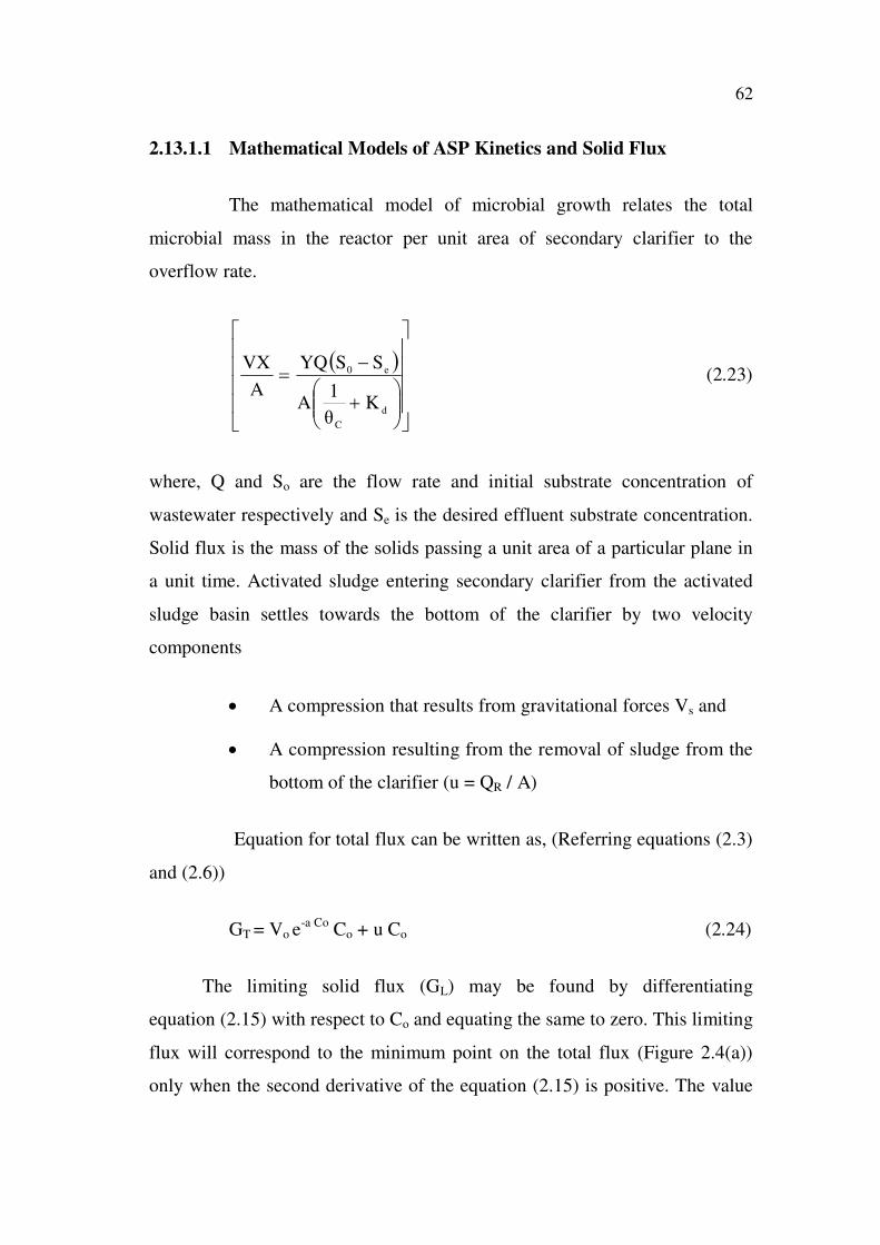
2.13.1.1 Mathematical Models of ASP Kinetics and Solid Flux
The mathematical model of microbial growth relates the total
microbial mass in the reactor per unit area of secondary clarifier to the
overflow rate.
d
C
e0
K1
A
SSYQ
A
VX (2.23)
where, Q and So are the flow rate and initial substrate concentration of
wastewater respectively and Se is the desired effluent substrate concentration.
Solid flux is the mass of the solids passing a unit area of a particular plane in
a unit time. Activated sludge entering secondary clarifier from the activated
sludge basin settles towards the bottom of the clarifier by two velocity
components
A compression that results from gravitational forces Vs and
A compression resulting from the removal of sludge from the
bottom of the clarifier (u = QR / A)
Equation for total flux can be written as, (Referring equations (2.3)
and (2.6))
GT = Vo e-a Co
Co + u Co (2.24)
The limiting solid flux (GL) may be found by differentiating
equation (2.15) with respect to Co and equating the same to zero. This limiting
flux will correspond to the minimum point on the total flux (Figure 2.4(a))
only when the second derivative of the equation (2.15) is positive. The value

63
of GL represents the maximum allowable flux loading, if the settling is to be
successful. If the influent flux to the settler is larger than GL, the sludge
blanket will rise resulting in solids in the effluent.
The limiting solids concentration corresponding to GL is,
5..0
o
2
2
o
2
o
LaR
CR1
R4
CR1
R2
CR1C (2.26)
The critical recycling ratio is given by,
o
o
C
Ca
4
CR 2.27)
For the Secondary Settling Tank to satisfy the thickening criteria,
flux applied to it must not exceed the limiting flux. Equating applied flux and
limiting flux, the design equations for calculating overflow rate to prevent
secondary clarifier deviating from its thickening performance are obtained as
below (Antonio et al 1987).
2
o
L
aC
o
C)R1(
aC.eV
A
Q L
for R < RC (2.28)
Re
V
A
Q2
o for R = RC (2.29)
0aC
0eVA
Q for R > RC (2.30)
2.13.2 Dynamic-State Control or Short-Term Control Strategies
These strategies are adopted when the plant faces short-term
variations in wastewater characteristics, resulting mainly from hydraulic
surge. The dynamic-state control is affected through the distribution of solids

64
between the aeration tank and the secondary settling tank by adjusting the
recycling ratio. The adjustment of recycling ratio is normally based on the
operational experience, gained over a variety of operating conditions and the
settling characteristics of the MLSS.
The operating conditions do not remain the same at all times, and
hence the behavior of the secondary clarifier often changes under different
operating scenarios. The state point represents the operating point of a
clarifier and it is very essential that the plant operator must continuously
monitor the state points of a clarifier and immediately take corrective
measures, when the state point deviates from the normal conditions. The state
point is analyzed with a help of a graph drawn between solid flux and solid
concentration. The state point is defined by the intersection of two operating
lines on the batch flux curve (point A in 2.4b). One of the lines has a slope of
–u and describes the recycle flow (under flow operating line) from the
clarifier to the aerator. The other begins at the origin and has a slope
equivalent to the clarifier over flow rate Q/A. Accordingly the state point has
the co- ordinates (Go Co) ( Figure 2.4 (b)). The batch settling flux approach
can be used to monitor the operational state of an activated sludge system
Keinath (1985) proposed two solids inventory control strategies for
prevention of clarification failure in the ASP. It was also suggested that
clarification failure could be prevented by adopting two types of control
strategies; recycle rate control and step feed control. Recycle rate control
strategy was shown to be effective for thickening over load and certain class
of thickening and clarification over loads. The step feed control strategy in
which location of feed point to the aeration tank by multiple basin at down
stream was shown to be effective, when the ASP experiencing severe
hydraulic surges.

65
Don Hee Park et al (1995) analyzed the data describing aerated
synthetic wastewater treated in a CFSTR, to understand the dynamic response
to step changes in the dilution rate D. The change in D between steady state
leading to hysteresis trajectories on both graph of specific growth rate (µ) Vs
limiting substrate level (S) and the graph of S Vs the cell level (X) were
compared for three different monitored cases and obtained a simple model at
various dilution level changes, in order to gain understanding of the dynamic
in the ASP.
Chancelier et al (1997) proposed an ordinary differential equation
that reproduced the dynamic behavior of the position of a shock between pure
water and concentrated sludge and formulated certain control laws to stabilize
the sludge blanket at a prescribed depth. The evolution of the sizes with small
particles flocculating into big ones and the residence time of particles in the
settler were considered in the model.
Saseetharan et al (1998) investigated the behavior of SST that
controlled the ASP operating in a dynamically changing environment by
adjusting the recycle rate to provide the required biomass concentration in the
aeration tank. The state point concept was used to adjust the recycling ratio.
The recycling ratio and the desired underflow concentration were chosen as
the influencing parameters. Mathematical models were developed to
determine the new recycle ratio in case of fluctuations in flow rate, substrate
concentration or both.
William et al (1999) carried out tests at a dry weather design flow
activated sludge plant of capacity 190 m3
/ h. The height of the sludge blanket
was measured and the return sludge rate was fine tuned to the desired rate.
The storm surge was simulated by controlling the drain valve in the storage
aeration basin. Results obtained during this study reflected the behavior of
clarifiers over a period of time during high hydraulic loading. The behavior of

66
the sludge blanket in the clarifier and the effluent suspended solids
concentration were studied extensively.
Takacs et al (2003) presented a dynamic model of the clarification
thickening process. Based on the solids flux concept and on a mass balance
around each layer of a one dimensional settler, the model could simulate the
solids profile throughout the settling column, including the underflow and
effluent suspended solids concentrations under steady state and dynamic
conditions. The model made use of a special settling velocity equation
designed to simulate the settling velocity of dilute and more concentrated
suspension. Results of the analysis confirmed that the model could serve to
predict the effluent and underflow suspended solids concentrations under
variety of conditions. .
2.13.2.1 Variable Influent Flowrate
All wastewater treatment plants experience short, intermediate and
long term fluctuations in influent flowrate. The operational state of the plant
correspondingly change due to fluctuations in the influent flowrate and plant
operator must immediately respond and take remedial measures to restore the
normal functioning of the plant. Whenever fluctuations cause an increase in
flowrate, state point gets shifted upwards from A to B in figure 2.8for certain
period of time, reactor MLSS remain the same.
Unaltered recycle flowrate may lead to an over loaded clarified
(dash double dotted line in Figure 2.8). The control can be exercised by
adjusting the recycle rate (i.e.) by making the recycle line (dotted line in
Figure 2.8) pass through the new state point B tangential to this flux curve
(Keinath et al 1977).

67
C0 CU
A
Q1/A
MLSS Concentration g/L
Soli
d F
lux K
g/m
².hr
GL'
GL
C0'
D
B
C
CU'
Q3/A
Q2/A
Figure 2.8 Loci of state points resulting from changes in hydraulic flow rate
2.13.2.2 Decreased Hydraulic Flowrate
In the case of decreased influent flowrate, the state point will shift
downwards (point D in Figure 2.8) at the same MLSS. If the plant operator
does not respond to the change of influent flowrate, a recycle operating line
will be parallel to the original line. However, for the operational state, the
clarifier is under loaded (dash - dot line in figure 2.8). The recycle rate can
accordingly be reduced to the point of critical loading. The control action is
beneficial, as it results in lowering of pumping cost and reduces turbulence in
clarifier, which should in turn result in upgraded clarification efficiencies.
2.13.2.3 Variable Substrate Concentration
From Figure 2.9, if at a given flowrate, conditions are such that the
state point of an activated sludge process is at ‘A’, the clarifier-thickener is
critically loaded (the operating line falling tangent to the flux curve). Then an
increase in substrate concentration in the influent provides the potential for an
increase in the suspended solids concentration in the aeration basin.

68
C 01 C U
A
Soli
d F
lux
Kg/m
².h
r
G L '
G L
C 0
B
C U '
1
C
C 02
MLSS Concentration, kg/m3
Figure 2.9 Loci of state points resulting from changes in substrate
concentration
However, because the clarifier-thickener is critically loaded, solids
begin to accumulate in the unit and the expected increase in solids
concentration in the aeration basin fails to materialize. If unchecked, the
accumulation will continue until the storage capacity of the clarifier-thickener
is depleted and solids are discharged in the overflow. The solids concentration
in the aeration basin can be increased only by increasing the recycle rate.
Such a situation is represented by state point ‘B’ and the steepest operating
line in Figure 2.9. As indicated by point ‘C’ in the figure, the reverse response
takes place when the substrate concentration decreases.
2.13.2.4 Variable Influent Flow and Substrate Concentration
In practice, changes in hydraulic flowrate and in substrate
concentration occur simultaneously and their effects are additive. The state
points corresponding to the critically loaded condition and over loaded
condition are shown in Figure 2.10 and the adjustment to be done in the
recycling ratio to avoid process failure is also shown. If the flow rate

69
increases by ‘n’ times, n (Q/A) = Q1/A and substrate increases by ‘n’ times to
n S, the combined effect of substrate and flow increase locate the new state
point at ‘C’ indicating a overloaded clarifier. The system response would be a
shift from ‘C’ to ‘D’ with time.
C 0 1 C U
A
M L S S C o nc entration g /L
So
lid
Flu
x K
g/m
².hr
G L '
G L
C 0
C
C U '
Q 1 /A
D
C 02
Q /A
B
Figure 2.10 Loci of state points resulting from flow rate and substrate
variation
The operator response at this situation would be to increase the
RAS rate, so that the recycle operating line (underflow operating line) passes
through ‘C’ and is tangential to the solid flux curve (dotted line in Figure 2.10).
2.14 OPERATIONAL DIAGRAMS FOR SECONDARY
CLARIFIERS
Daigger and Roper (1985) correlated batch settling test data with
SVI for estimating activated sludge settling characteristics. The following
relationship was determined

70
iC)SVI(00210.0148.0
e80.7Vi
(2.31)
where Vi = Initial settling velocity corresponding to the concentration Ci .
Using this equation, clarifier design and operating criteria were
developed for SVIs ranging from 50 mL/g to 350 mL/g in increments of 50
mL/g. Clarifier design and operating diagrams were presented, which allowed
the design engineers and plant operators to apply settling flux theory easily
and directly. It is interpreted from the chart that, for a constant return sludge
flow rate, state point will move upward when plant flow / MLSS increases.
Increasing RAS flow rate will shift the operating line upward.
Keinath (1990) developed a broadly applicable design and
operations chart for use by design engineers and wastewater treatment plant
operators. A regression characterizing the settleability of biological solids
developed, using experimental batch settling data collected at 21 full scale
wastewater treatment plants of different types was used to develop the chart.
The design examples showed that, the chart could be used with ease for
designing a secondary clarifier according to the thickening criterion and
evaluating various economic trades-off to determine a cost effective design.
The operation examples showed how return sludge flowrate or step feed
control strategies could be implemented to ameliorate thickening over loaded
conditions in an operating secondary clarifier.
Daigger (1995) developed a refined clarifier operating diagrams
using an updated settling characteristics data base. The results from the
analysis of five sets of settling characteristics representing 51 separate
suspended growth biological wastewater treatment processes indicated that
the data could be characterized using a single relationship between the initial
settling velocity, the initial sludge concentration and the sludge volume index.

71
These results suggested that this single relationship could be used to
accurately characterize the settling characteristics of an activated sludge based
only on the measured SVI. Based on the developed relationship the
secondary clarifier operating diagrams were presented.
Hermanowicz (1998) presented operational diagrams that were
developed in a unified way, relating the operating parameters of activated
sludge operation. The diagrams explicitly and directly related the MLSS and
RAS concentrations with the recycle ratio and clarifier hydraulic loading. The
diagrams could be used to evaluate operational control options and to design
secondary clarifiers. A procedure was also presented to develop a modified
diagram, based on a specific relationship between solids concentration and
settling velocity. This procedure could be used to customize the diagrams in
response to changes in solids settling characteristics.
Richard et al (2001) compared the settling characteristics of mixed
liquor produced by different types of biological treatment processes.
Experimental SVI values fitted well with the equation proposed by Daigger
(1985). A secondary clarifier operating diagram was also developed at uSVI’s
of 100, 150 and 200 mL/g, relating MLSS, RAS, R and hydraulic loading.
The charts could be used by the treatment plant operators for determining
appropriate recycle and wastage rates or by consultants for designing
secondary clarifiers.
Giokas et al (2003) made an investigation on the real-time
database of zone settling data sets. In order to correlate the design and
simulation of secondary clarifiers, zone settling velocity parameters, unstirred
SVI, stirred SVI and sludge blanket height were considered. For Design
purpose, an update of the existing generalized values of settling velocity
parameters was proposed. Using the database solid flux and overflow rate
diagrams were prepared.
72
Jeyanthi and Saseetharan (2007) developed an operational diagram
for the process control of the secondary clarifier for treating dairy wastewater
with a MCRT of 11 days, subsequent to the determination of mathematical
models for the surface area of the settler. It was claimed that the diagram
could be used to design secondary clarifier and evaluate operational control
options in response to changes in flow rate on solids settleability
2.15 CRITICAL REVIEW
Many research works in activated sludge process have been carried
out that have improved the system efficiency. Most of the works are related to
the design of ASP as a whole unit. Mathematical models that were developed
earlier, did not offer greater importance to the design of clarifier. Especially,
the variations in the operating conditions were not considered in the system
design, with an exception that an excess factor of safety was assumed to take
care of such occasional variations. But subsequently few scholars like
Keinath (1990), Saseetharan et al (1997), Jeyanthi and Saseetharan. (2006)
besides developing mathematical models, provided operational diagrams to
facilitate the design and operation of secondary clarifier. Richard. O Mines
(2001) also presented secondary clarifier operational diagrams. Wahl Berg
et al (1994) provided the state point analysis for making timely process
control decision for activated sludge plant operation. Keinath (1997)
presented a detailed analysis on the state point concept and formulated control
strategies to tackle the over loading of clarifiers. Hermanowicz (1998)
developed easily readable operating diagrams for the secondary clarifier
solids flux theory and zone settling velocity. Jeyanthi and Saseetharan (2006)
developed models and operational diagrams for the secondary clarifier
treating combined dairy and domestic waste waters.
All the above works in the secondary clarifiers have been carried
out envisaging the variations in operating conditions viz., influent flowrate,

73
substrate concentration and combination of both. But so far, not much of
works seem to have been carried out in the design of secondary clarifier and
the operational diagrams, considering the most important and common
problems of filamentous bulking in the clarifier. Although, Jenkins et al
(1993), Michael Richard (1993) and Eikel Boom (1995) have identified the
causes of filamentous bulking and the control measures to combat the
bulking; the same has not been incorporated in the design of secondary
clarifier.
2.16 SCOPE OF THE RESEARCH
The secondary clarifier is an integral unit of activated sludge
process and often determines the capacity and the efficiency of the treatment
plant. The functioning of secondary clarifier is interrelated with the
functioning of the aerator. The failure to consider this interdependency
between the aerator and the clarifier will lead to poor clarifier design and
operation. The design of secondary clarifier will not be complete and perfect
without considering the fluctuations in operating parameters like influent
flowrate, variations in substrate concentrations and the combination of both.
Necessary remedial measures are required to take care of occasional, seasonal
and sudden variations in such operating parameters. It is equally essential
that the filamentous bulking, the most common problem in the secondary
clarifier must be duly addressed while designing and operating the secondary
clarifier.
Hence in the research, the coupled system of aerator and secondary
clarifier were studied using Monod’s kinetics of activated sludge, solids flux
models along with addition of optimum dosages of chlorine in combating the
filamentous bulking. Before taking up the study, a clear understanding was
made on the bacteriological activities by identifying the predominant
biodegrading bacteria present in the dairy wastewater.

74
The effect of the native bacterial isolates in the treatment of dairy
wastewater was studied by inoculating the bacterial isolates in different
strength. The optimum parameters like pH, temperature and incubation time
were standardized for maximum enzyme production, which facilitated the
bacterial growth, in the aerator. While facilitating the biodegrading
functioning in the aerator, the filamentous organisms responsible for bulking
in the clarifier was also studied. The optimum dosages of chlorine that would
control the filamentous bulking without affecting the biodegrading bacteria,
for different MCRT were studied.
The models and the operational diagrams were extended with those
of Daigger and Roper (1985), Keinath (1990), Saseetharan et al (1997),
Hermanowicz (1998), Richard et al (2001), Jeyanthi and Saseetharan (2006)
incorporating the bulking control with the addition of chlorine in the clarifier
and relating all of the process control parameters in simple graphical forms.
The scope of this research was taken in different phases and the
results are presented separately one after another. However, the methodologies in
carrying out the different experiments are grouped together and presented in
chapter 3.
Top Related