


Languages
Pages
Legal


LEARNING AND INFERENCE IN GRAPHICAL MODELS
Chapter 11: Markov Logic Networks
Dr. Martin Lauer
University of FreiburgMachine Learning Lab
Karlsruhe Institute of TechnologyInstitute of Measurement and Control Systems
Learning and Inference in Graphical Models. Chapter 11 – p. 1/28

References for this chapter
◮ Matthew Richardson and Pedro Domingos, Markov logic networks. In:Machine Learning, vol. 62, no. 1-2, pp. 107-136, 2006
Learning and Inference in Graphical Models. Chapter 11 – p. 2/28

Logic and probabilities
Two perspectives on artificial intelligence:
Logical reasoning
◮ knowledge is stored in logicalformulas
◮ a logical formula is either true orfalse
◮ the world is sure
◮ the world is repeatable
◮ logical calcultio
Probabilistic reasoning
◮ knowledge is stored in jointprobability distributions
◮ we never know the exact value of arandom variable
◮ the world in unsure
◮ repetitions of an experiment yielddifferent results
◮ stochastic inference procedures
Can we combine logical and probabilistic reasoning?
Learning and Inference in Graphical Models. Chapter 11 – p. 3/28

Propositional logic
In propositional logic we have:
◮ Boolean variables a, b, . . .
◮ formulas created by combining Boolean variables (including true, false) withconnectors¬a, a ∧ b, a ∨ b, a→ b, a↔ b
◮ an interpretation is an assignment of Boolean variables to either true orfalse
◮ a model of a set of formulae is an interpretation for which all formulaeevaluate to true
Can we represent a set of propositional formulae in a MRF?
Learning and Inference in Graphical Models. Chapter 11 – p. 4/28

Markov logic networks
Let G = {g1, . . . , gn} be a set of Boolean functions over variables a1, . . . , ak
We create a factor graph with
◮ k binary variable nodes B1, . . . , Bk
◮ n factor nodes F1, . . . , Fn
◮ Bj is connected with Fi if Boolean variable aj occurs in formula gi
◮ we define potential functions for factor Fi as followsif Fi is connected to B
j(i)1, . . . , B
j(i)N
ψi(bj(i)1, . . . , b
j(i)Ni
) =
e1 if formula gi is satisfied for an interpretation
that maps al onto true if and only if bl = 1
e0 otherwise
The MRF that refers to this factor graph is called a Markov logic network (MLN)
Learning and Inference in Graphical Models. Chapter 11 – p. 5/28

Markov logic networks
For simplicity of notation, let us introduce
g̃i(bj(i)1, . . . , b
j(i)Ni
) :=
1 if formula gi is satisfied for an interpretation
that maps al onto true if and only if bl = 1
0 otherwise
Hence, potential functions can be written as
ψi(bj(i)1, . . . , b
j(i)Ni
) = eg̃i(b
j(i)1
,...,bj(i)Ni
)
Learning and Inference in Graphical Models. Chapter 11 – p. 6/28

Markov logic networks
Example:
g1 : a1 ∨ a2
g2 : a2 → a3
g3 : ¬a3
Potential functions:
ψ1(b1, b2) =
{
e if b1 + b2 ≥ 1
1 otherwise
ψ2(b2, b3) =
{
e if b3 − b2 ≥ 0
1 otherwise
ψ3(b3) =
{
e if b3 = 0
1 otherwise
B1
B2
B3
�F1 �F2 �F3
Learning and Inference in Graphical Models. Chapter 11 – p. 7/28
Markov logic networks
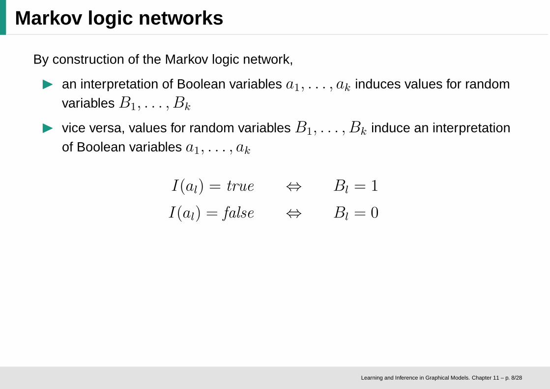
By construction of the Markov logic network,
◮ an interpretation of Boolean variables a1, . . . , ak induces values for randomvariables B1, . . . , Bk
◮ vice versa, values for random variables B1, . . . , Bk induce an interpretationof Boolean variables a1, . . . , ak
I(al) = true ⇔ Bl = 1
I(al) = false ⇔ Bl = 0
Learning and Inference in Graphical Models. Chapter 11 – p. 8/28

Markov logic networks
The joint probability of the Markov logic network:
p(b1, . . . , bk) =1
Z
n∏
i=1
ψi(bj(i)1, . . . , b
j(i)Ni
)
=1
Ze
∑ni=1 g̃i(b
j(i)1
,...,bj(i)Ni
)
The joint probability counts the number of satisfied formulae.
Conclusions:
1. If I is a model of the set of formulae, then the the induced values of Bi arethe maximum-a-posterior estimator.
2. If the set of formulae is satisfiable, then the maximum-a-posterior estimatorof the MLN induces a model.
3. If the set of formulae is unsatisfiable, then the maximum-a-posteriorestimator of the MLN induces an interpretation which satisfies as manyformulae as possible.
Learning and Inference in Graphical Models. Chapter 11 – p. 9/28

Complexity of finding the MAP
Remark:From the previous result we can conclude that determining the MAP estimator inan MRF is NP-hard.
Proof:We know that the satisfiability problem (SAT) is NP-complete.The construction of a MLN from a set of formulae can be done in polynomial timeHence, finding the MAP estimator in a MLN is NP-hard (even more, it isNP-complete).Hence, the complexity of finding the MAP estimator in a general MRF is NP-hard.
Learning and Inference in Graphical Models. Chapter 11 – p. 10/28

Markov logic networks
a1 a2 a3 b1 b2 b3 I(g1) I(g2) I(g3) p(·)
false false false 0 0 0 false true true 1Ze2
false false true 0 0 1 false true false 1Ze1
false true false 0 1 0 true false true 1Ze2
false true true 0 1 1 true true false 1Ze2
true false false 1 0 0 true true true 1Ze3
true false true 1 0 1 true true false 1Ze2
true true false 1 1 0 true false true 1Ze2
true true true 1 1 1 true true false 1Ze2
B1
B2
B3
�F1 �F2 �F3
g1 : a1 ∨ a2
g2 : a2 → a3
g3 : ¬a3
Learning and Inference in Graphical Models. Chapter 11 – p. 11/28
Markov logic networks
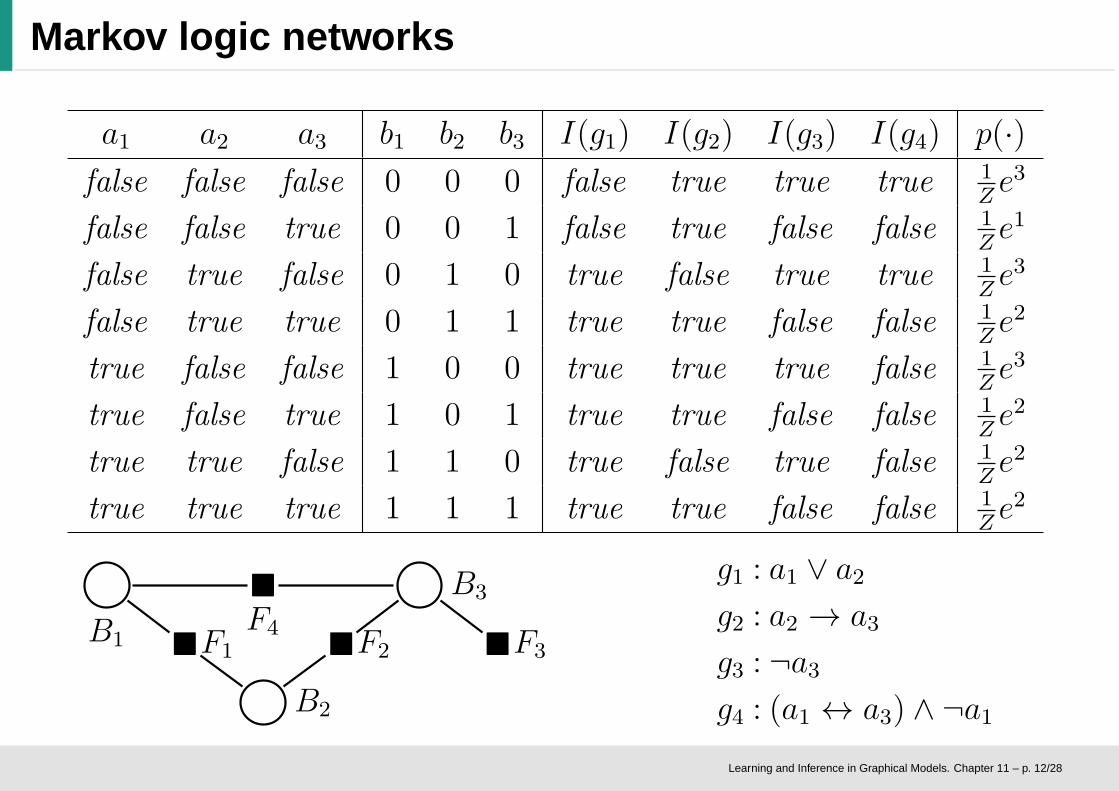
a1 a2 a3 b1 b2 b3 I(g1) I(g2) I(g3) I(g4) p(·)
false false false 0 0 0 false true true true 1Ze3
false false true 0 0 1 false true false false 1Ze1
false true false 0 1 0 true false true true 1Ze3
false true true 0 1 1 true true false false 1Ze2
true false false 1 0 0 true true true false 1Ze3
true false true 1 0 1 true true false false 1Ze2
true true false 1 1 0 true false true false 1Ze2
true true true 1 1 1 true true false false 1Ze2
B1
B2
B3
�F1 �F2 �F3
�
F4
g1 : a1 ∨ a2
g2 : a2 → a3
g3 : ¬a3
g4 : (a1 ↔ a3) ∧ ¬a1
Learning and Inference in Graphical Models. Chapter 11 – p. 12/28

Markov logic networks
The unsatisfiable case is most interesting since it is typical in real-worldapplications.
◮ we have a set of formulae which describe vague knowledge
◮ we want to infer which interpretation is “most likely”
◮ some formulae might be more important or less unsure than others
Learning and Inference in Graphical Models. Chapter 11 – p. 13/28
Markov logic networks
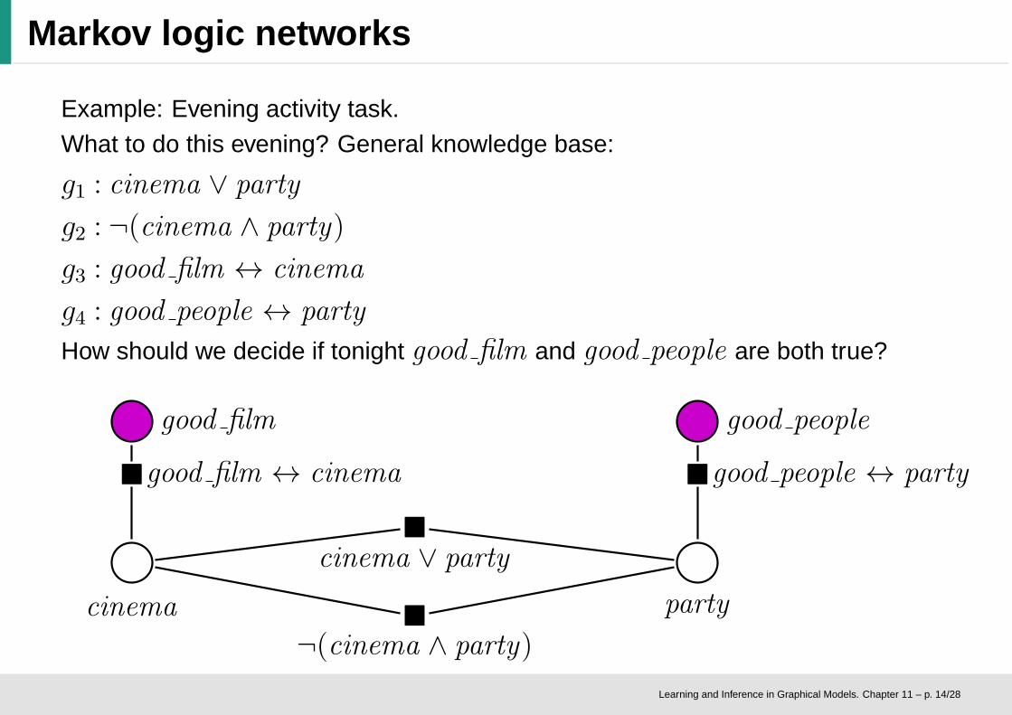
Example: Evening activity task.What to do this evening? General knowledge base:
g1 : cinema ∨ party
g2 : ¬(cinema ∧ party)
g3 : good film ↔ cinema
g4 : good people ↔ party
How should we decide if tonight good film and good people are both true?
good film
�good film ↔ cinema
cinema
good people
�good people ↔ party
party
�
cinema ∨ party
�
¬(cinema ∧ party)
Learning and Inference in Graphical Models. Chapter 11 – p. 14/28

Markov logic networks
Example: Evening activity task.Let us assume some of the rules are more important to us than others, e.g.
g1 : cinema ∨ party (not important, w1 = 1)
g2 : ¬(cinema ∧ party) (very important, cannot do both, w2 = 9)
g3 : good film ↔ cinema (not that important, w3 = 3)
g4 : good people ↔ party (important, w4 = 6)
Let us model importance of rules with non-negative weights.
Modify potential functions:
ψi(bj(i)1, . . . , b
j(i)Ni
) = ewig̃i(b
j(i)1
,...,bj(i)Ni
)
Now, the exponent in the joint probability sums the weights of satisfied formulae.
How should we decide if tonight good film and good people are both true?
→ go to party since MAP yields 1Ze16 (party) instead of 1
Ze13 (cinema)
Learning and Inference in Graphical Models. Chapter 11 – p. 15/28
Learning in Markov logic networks
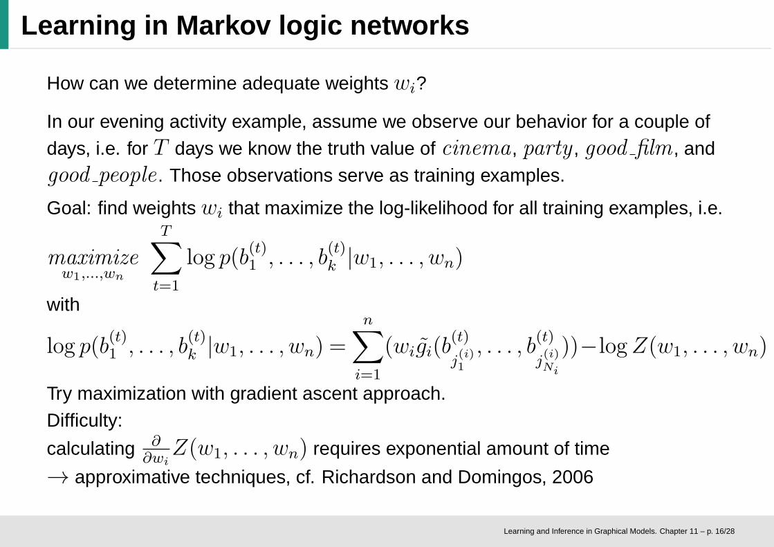
How can we determine adequate weights wi?
In our evening activity example, assume we observe our behavior for a couple ofdays, i.e. for T days we know the truth value of cinema , party , good film , andgood people . Those observations serve as training examples.
Goal: find weights wi that maximize the log-likelihood for all training examples, i.e.
maximizew1,...,wn
T∑
t=1
log p(b(t)1 , . . . , b
(t)k |w1, . . . , wn)
with
log p(b(t)1 , . . . , b
(t)k |w1, . . . , wn) =
n∑
i=1
(wig̃i(b(t)
j(i)1
, . . . , b(t)
j(i)Ni
))−logZ(w1, . . . , wn)
Try maximization with gradient ascent approach.Difficulty:
calculating ∂∂wi
Z(w1, . . . , wn) requires exponential amount of time
→ approximative techniques, cf. Richardson and Domingos, 2006
Learning and Inference in Graphical Models. Chapter 11 – p. 16/28

Learning in Markov logic networks
Special case: we only have one logical fomula g1.
Goal: calculate the gradient of log p(b(t)1 , . . . , b
(t)k |w1)
log p(b(t)1 , . . . , b
(t)k |w1) = w1g̃1(b
(t)1 , . . . , b
(t)k )− logZ(w1)
with
Z1(w1) =∑
(b1,...,bk)∈{0,1}k
ewig̃i(b1,...,bk) = K+1 e
w1 +K−1
where
K+1 := |{b1, . . . , bk) ∈ {0, 1}k|g̃1(b1, . . . , bk) = 1}|
K−1 := |{b1, . . . , bk) ∈ {0, 1}k|g̃1(b1, . . . , bk) = 0}|
Learning and Inference in Graphical Models. Chapter 11 – p. 17/28
Learning in Markov logic networks
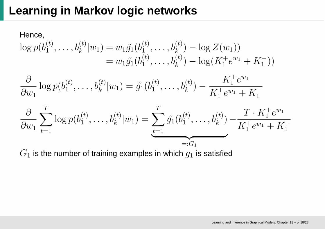
Hence,
log p(b(t)1 , . . . , b
(t)k |w1) = w1g̃1(b
(t)1 , . . . , b
(t)k )− logZ(w1))
= w1g̃1(b(t)1 , . . . , b
(t)k )− log(K+
1 ew1 +K−
1 ))
∂
∂w1
log p(b(t)1 , . . . , b
(t)k |w1) = g̃1(b
(t)1 , . . . , b
(t)k )−
K+1 e
w1
K+1 e
w1 +K−1
∂
∂w1
T∑
t=1
log p(b(t)1 , . . . , b
(t)k |w1) =
T∑
t=1
g̃1(b(t)1 , . . . , b
(t)k )
︸ ︷︷ ︸
=:G1
−T ·K+
1 ew1
K+1 e
w1 +K−1
G1 is the number of training examples in which g1 is satisfied
Learning and Inference in Graphical Models. Chapter 11 – p. 18/28
Learning in Markov logic networks
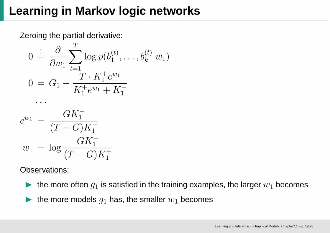
Zeroing the partial derivative:
0!=
∂
∂w1
T∑
t=1
log p(b(t)1 , . . . , b
(t)k |w1)
0 = G1 −T ·K+
1 ew1
K+1 e
w1 +K−1
· · ·
ew1 =GK−
1
(T −G)K+1
w1 = logGK−
1
(T −G)K+1
Observations:
◮ the more often g1 is satisfied in the training examples, the largerw1 becomes
◮ the more models g1 has, the smaller w1 becomes
Learning and Inference in Graphical Models. Chapter 11 – p. 19/28

Markov logic networks for propositional logic
Brief receipe of MLNs for propositional logic:
◮ creating and training a MLN
• create a set of propositional formulae that might contribute to a logicalinference
• collect training examples (the more the better)
• train the weights wi
◮ applying a MLN to a new situation
• determine all Boolean variables that you can observe
• apply inference procedures (e.g. Gibbs sampling) on the MLN to find theMAP estimator
• from the MAP estimator you can derive the best interpretation of thescene
Learning and Inference in Graphical Models. Chapter 11 – p. 20/28
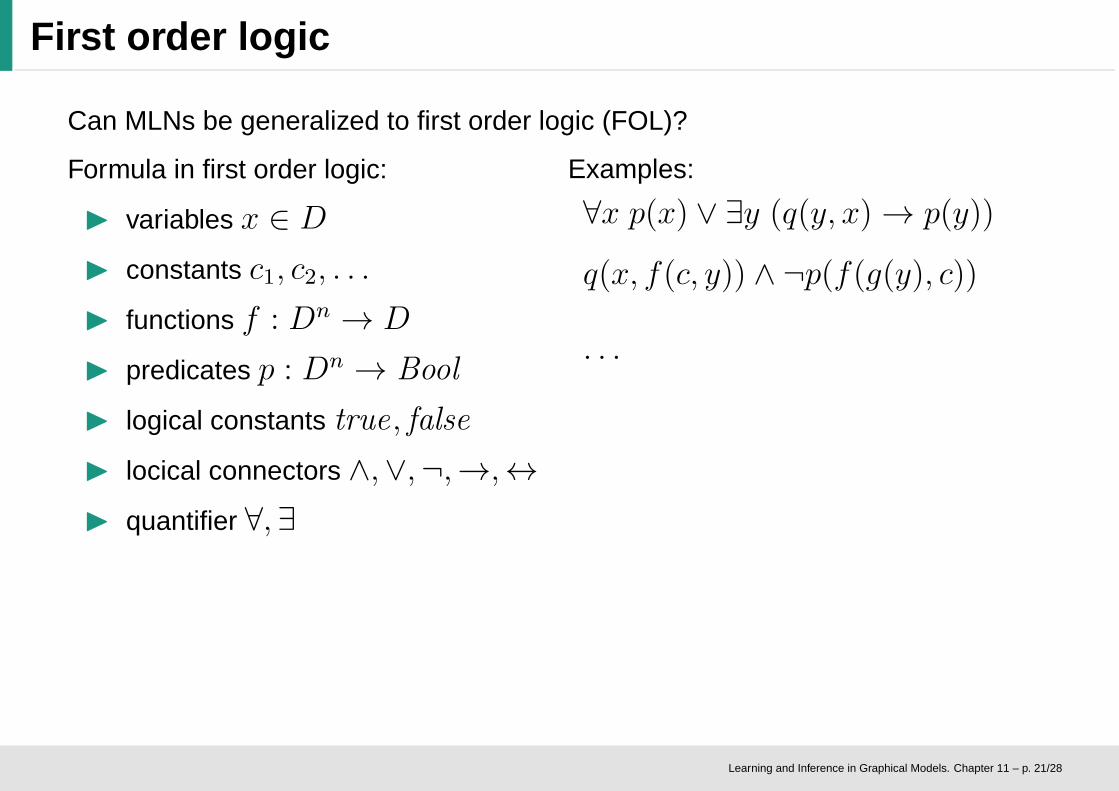
First order logic
Can MLNs be generalized to first order logic (FOL)?
Formula in first order logic:
◮ variables x ∈ D
◮ constants c1, c2, . . .
◮ functions f : Dn → D
◮ predicates p : Dn → Bool
◮ logical constants true, false
◮ locical connectors ∧,∨,¬,→,↔
◮ quantifier ∀, ∃
Examples:
∀x p(x) ∨ ∃y (q(y, x) → p(y))
q(x, f(c, y)) ∧ ¬p(f(g(y), c))
. . .
Learning and Inference in Graphical Models. Chapter 11 – p. 21/28
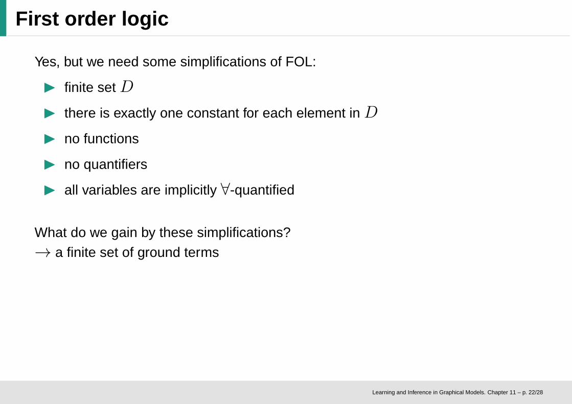
First order logic
Yes, but we need some simplifications of FOL:
◮ finite set D
◮ there is exactly one constant for each element in D
◮ no functions
◮ no quantifiers
◮ all variables are implicitly ∀-quantified
What do we gain by these simplifications?→ a finite set of ground terms
Learning and Inference in Graphical Models. Chapter 11 – p. 22/28

Grounding
Definition: a ground term is a formula that does not contain variables.
We can create a ground term from any formula by substituting variables byconstants. We can create all ground terms of a formula by applying all possiblesubstitutions to the formula.
Example:assume the only constants c1, c2 and formula p(x, y) → q(x)
groundings:
p(c1, c1) → q(c1)
p(c1, c2) → q(c1)
p(c2, c1) → q(c2)
p(c2, c2) → q(c2)
Every ground formula can be interpreted as a formula of propositional logic. Now,we can apply the MLN idea to all ground formulae of a set of FOL formulae.
Learning and Inference in Graphical Models. Chapter 11 – p. 23/28
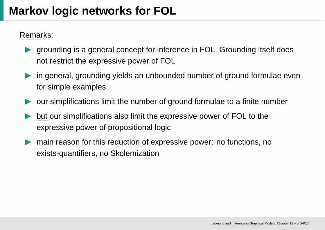
Markov logic networks for FOL
Remarks:
◮ grounding is a general concept for inference in FOL. Grounding itself doesnot restrict the expressive power of FOL
◮ in general, grounding yields an unbounded number of ground formulae evenfor simple examples
◮ our simplifications limit the number of ground formulae to a finite number
◮ but our simplifications also limit the expressive power of FOL to theexpressive power of propositional logic
◮ main reason for this reduction of expressive power: no functions, noexists-quantifiers, no Skolemization
Learning and Inference in Graphical Models. Chapter 11 – p. 24/28
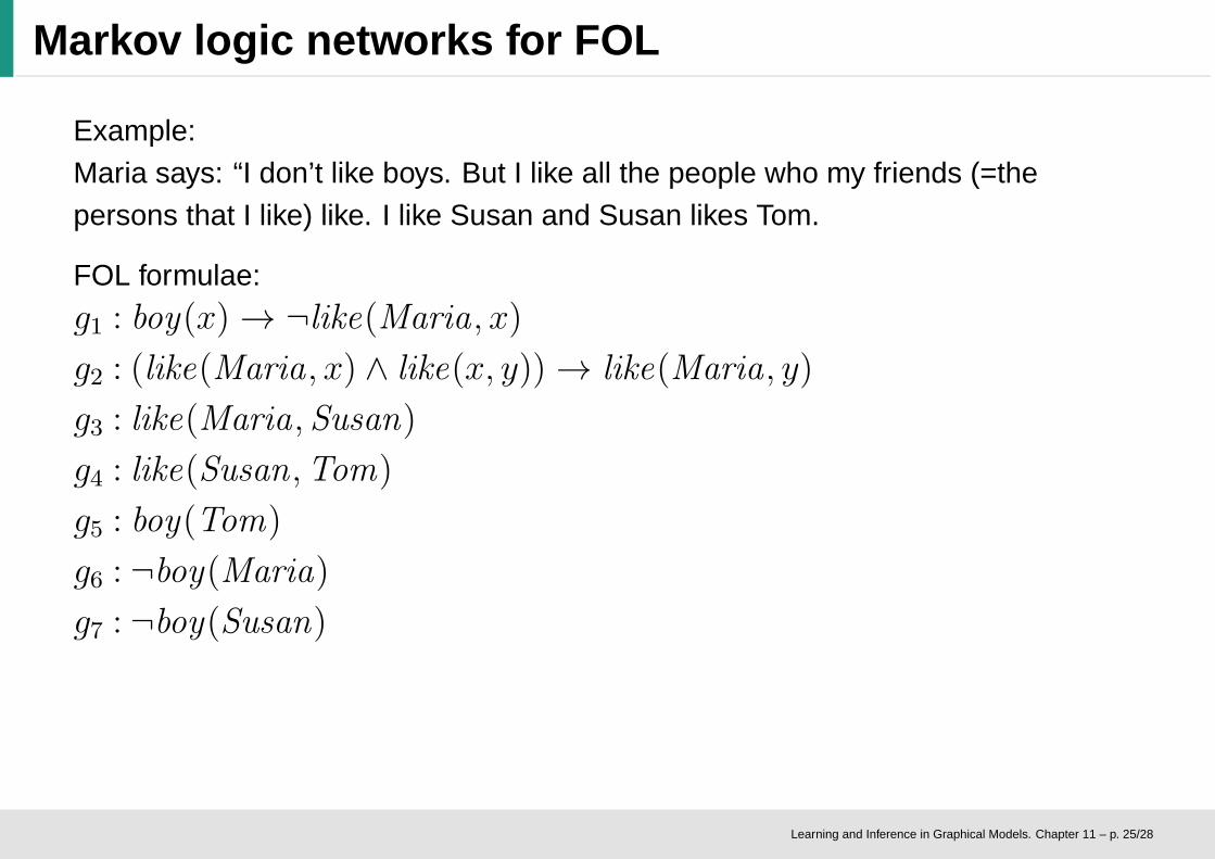
Markov logic networks for FOL
Example:Maria says: “I don’t like boys. But I like all the people who my friends (=thepersons that I like) like. I like Susan and Susan likes Tom.
FOL formulae:
g1 : boy(x) → ¬like(Maria, x)
g2 : (like(Maria, x) ∧ like(x, y)) → like(Maria, y)
g3 : like(Maria, Susan)
g4 : like(Susan,Tom)
g5 : boy(Tom)
g6 : ¬boy(Maria)
g7 : ¬boy(Susan)
Learning and Inference in Graphical Models. Chapter 11 – p. 25/28

Markov logic networks for FOL
g1,1 : boy(Tom) → ¬like(Maria,Tom)
g1,2 : boy(Susan) → ¬like(Maria,Susan)
g1,3 : boy(Maria) → ¬like(Maria,Maria)
g2,1 : (like(Maria,Tom) ∧ like(Tom,Tom)) → like(Maria,Tom)
g2,2 : (like(Maria,Tom) ∧ like(Tom,Susan)) → like(Maria,Susan)
g2,3 : (like(Maria,Tom) ∧ like(Tom,Maria)) → like(Maria,Maria)
g2,4 : (like(Maria,Susan) ∧ like(Susan,Tom)) → like(Maria,Tom)
g2,5 : (like(Maria,Susan) ∧ like(Susan,Susan)) → like(Maria,Susan)
g2,6 : (like(Maria,Susan) ∧ like(Susan,Maria)) → like(Maria,Maria)
g2,7 : (like(Maria,Maria) ∧ like(Maria,Tom)) → like(Maria,Tom)
g2,8 : (like(Maria,Maria) ∧ like(Maria,Susan)) → like(Maria,Susan)
g2,9 : (like(Maria,Maria) ∧ like(Maria,Maria)) → like(Maria,Maria)
g3 : like(Maria,Susan)
g4 : like(Susan,Tom)
g5 : boy(Tom)
g6 : ¬boy(Maria)
g7 : ¬boy(Susan)
Ground formulae
Important:ground formulaethat are createdfrom the sameformula sharetheir weights wi
Learning and Inference in Graphical Models. Chapter 11 – p. 26/28
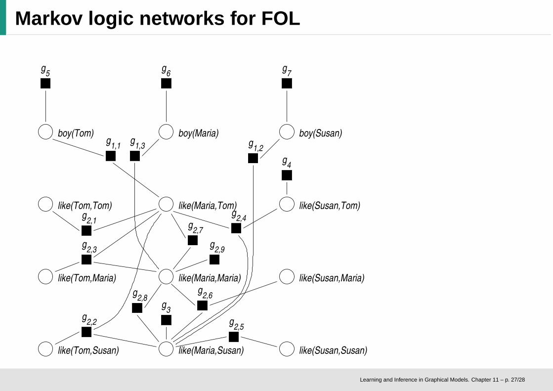
Markov logic networks for FOL
like(Maria,Maria)
like(Maria,Tom)
boy(Maria)boy(Tom) boy(Susan)
like(Tom,Susan) like(Maria,Susan) like(Susan,Susan)
like(Tom,Tom)
like(Tom,Maria) like(Susan,Maria)
like(Susan,Tom)
g7
g6
g5
g1,1 g
1,2g1,3
g2,3
g2,1
g2,2
g2,4
g2,5
g2,6
g2,7
g2,8
g2,9
g3
g4
Learning and Inference in Graphical Models. Chapter 11 – p. 27/28

Summary
◮ definition of Markov logic networks
◮ MAP estimators as logical models
◮ weighted formulae
◮ training a MAP from training examples
◮ extensions to first order logic
Learning and Inference in Graphical Models. Chapter 11 – p. 28/28
Top Related