


Languages
Pages
Legal


Yale ICF Working Paper No. 02-03 June 16, 2003
CAPITAL STRUCTURE AND STOCK RETURNS
Ivo Welch Yale School of Management
This paper can be downloaded without charge from the Social Science Research Network Electronic Paper Collection:
http://ssrn.com/abstract_id=298196

Forthcoming: Journal of Political Economy, February 2004
Capital Structure and Stock Returns∗
Ivo Welch
Yale and NBER
June 16, 2003
∗An earlier draft was titled “Columbus Egg.” I thank Judy Chevalier, Eugene Fama,Ken French, William Goetzmann, John Graham, David Hirshleifer, Gerard Hoberg, SteveKaplan, Florencio Lopez-De-Silanes, Vojislav Maksimovic, Roni Michaely, Gordon Philips,Mike Stutzer, Sheridan Titman, and many seminar participants for comments. JohnCochrane, in particular, gave me the best paper comments I have received in my career.Gerard Hoberg provided terrific research assistance. The author’s current web page ishttp://welch.som.yale.edu/.

Abstract
U.S. corporations do not issue and repurchase debt and equity to counteract
the mechanistic effects of stock returns on their debt equity ratios. Thus, over
1–5 year horizons, stock returns can explain about 40% of debt ratio dynamics.
Although corporate net issuing activity is lively, and although it can explain
60% of debt ratio dynamics (long-term debt issuing activity being most capital
structure relevant), corporate issuing motives remain largely a mystery. When
stock returns are accounted for, many other proxies used in the literature, play
a much lesser role in explaining capital structure.

I Introduction
This paper shows that U.S. corporations do little to counteract the influence of stock
price changes on their capital structures. As a consequence, their debt equity ratios
vary closely with fluctuations in their own stock prices. The stock price effects are
often large and long-lasting, at least several years.
This paper decomposes capital structure changes into effects caused by cor-
porate issuing net of retirement activity (henceforth, called “net issuing” or just
“issuing”), and into effects caused by stock returns. While all stock-return caused
equity growth can explain about 40% of capital structure dynamics, all corporate
issuing activity together can explain about 60% to 70%. Long-term debt issuing is
the most capital-structure relevant corporate activity, explaining about 30% of the
variation in corporate debt ratio changes.
However, the corporate issuing motives themselves remain largely a mystery.
Issuing activities are not used to counterbalance stock-return induced equity value
changes. The better known proxy variables used in the literature—such as tax costs,
expected bankruptcy costs, earnings, profitability, market-book ratios, uniqueness,
market timing, or the exploitation of undervaluation—also fail to explain much cap-
ital structure dynamics when stock value mechanics are accounted for. In previous
work, these proxies passively correlated with debt ratios primarily indirectly, be-
cause they correlated with omitted stock return caused dynamics. Put differently,
these proxies have not so much induced managers to actively engage in altering
their capital structures, as much as they have allowed firms to experience different
equity values and therefore different capital structures. The proactive managerial
component in capital structure remains largely unexplained.
The paper concludes that over reasonably long time frames, the stock price ef-
fects are considerably more important in explaining debt-equity ratios than previ-
ously identified proxies. Stock returns are the primary known component of capital
structure and capital structure changes.
1

II Capital Structure Ratios
My paper investigates whether actual debt ratios by-and-large behave as if firms
readjust to their previous debt ratios (targeting a largely static target), or whether
they permit their debt ratios to fluctuate with stock prices. The basic specification
estimates
ADRt+k = α0 +α1 · ADRt +α2 · IDRt,t+k + εt . (1)
ADR is the actual corporate debt ratio, defined as the value of debt (D) divided by
the value of debt plus equity (E),
ADRt ≡Dt
Et +Dt, (2)
and has been the dependent variable in many capital structure papers. ADR is also a
component of the weighted average cost of capital (WACC). IDR is the implied debt
ratio that comes about if the corporation issues (net) neither debt nor equity,
IDRt,t+k ≡Dt
Et · (1+ xt,t+k)+Dt, (3)
where x is the stock return net of dividends. (Whether dividends are included
matters little in this study.)
The stark hypotheses are
Perfect Readjustment Hypothesis: α1 = 1 α2 = 0 ,
Perfect Non-Readjustment Hypothesis: α1 = 0 α2 = 1 .(4)
Firms could also adopt convex combination strategies, more appropriate than these
two “straw man” extremes, and different firms could behave differently. If included,
the intercept α0 can capture a constant target debt ratio. The empirical specifica-
tions are primarily cross-sectional.
2
The dynamics of capital structure that underlie specification (1) can be expressed
as follows. The amount of debt changes with new debt issues, debt retirements,
coupon payments, and debt value changes. Corporate debt evolves as
Dt+k ≡ Dt + TDNIt,t+k , (5)
where TDNI is the total debt net issuing activity. Equivalently, the amount of cor-
porate equity changes with stock returns (net of dividends), and new equity issues
net of equity repurchases. Corporate equity evolves as
Et+k ≡ Et · (1+ xt,t+k)+ ENIt,t+k , (6)
where ENI is net equity issuing and stock repurchasing activity. Using these defini-
tions, debt ratios evolve as
ADRt+k = Dt+kEt+k +Dt+k
= Dt + TDNIt,t+kDt + TDNIt,t+k + Et · (1+ xt,t+k)+ ENIt,t+k
. (7)
Mathematically, if the corporation issues debt and equity so that
ENIt,t+kEt
=(
TDNIt,t+kDt
)− xt,t+k , (8)
then ADR remains perfectly constant across periods (ADRt+k = ADRt ⇒ α1 = 1, α2 =0). In contrast, if the corporation issues debt and equity so that
ENIt,t+kEt
=(
TDNIt,t+kDt
)+ xt,t+k ·
(TDNIt,t+k
Dt
), (9)
then IDR perfectly predicts debt ratios (IDRt,t+k = ADRt ⇒ α1 = 0, α2 = 1). Un-
fortunately, equations 8 and 9 are unsuitable for direct cross-sectional estimation,
because many firms have zero or tiny debt levels.
3
III Data
My data set begins with all publicly traded U.S. corporations from the period 1962
to 2000 from the Annual Compustat and CRSP files. The paper predicts debt ratios
for all firm-years that have an initial equity market capitalization of at least the
S&P500 level divided by 10 (in year t, not t+k!). So, in 1964, the first year for which
I predict debt ratios, the minimum market capitalization is $75 million; in 2000, it
is $1.47 billion. Nevertheless, the number of sample firms grows from 412 in 1964
to 2,679 in 2000. In total, 60,317 firm-years qualify, but only 54,211 firm-years have
data in two consecutive years, and only 40,080 firm-years have data over five years.
The results are robust when the firm size filter is varied or even eliminated.
D is the Compustat book value of debt. E is the CRSP market value of equity. x
is the CRSP percent price change in the market-value of equity and differs slightly
from r (the stock rate of return) due to dividends. In Tables 1, 2, and 4, TDNI and ENI
are computed from D and E dynamics, respectively. All issuing activity in this paper
is “net”—there is no data to separate issuing from retiring activity. More detailed
data definitions and method descriptions are in the Appendix.
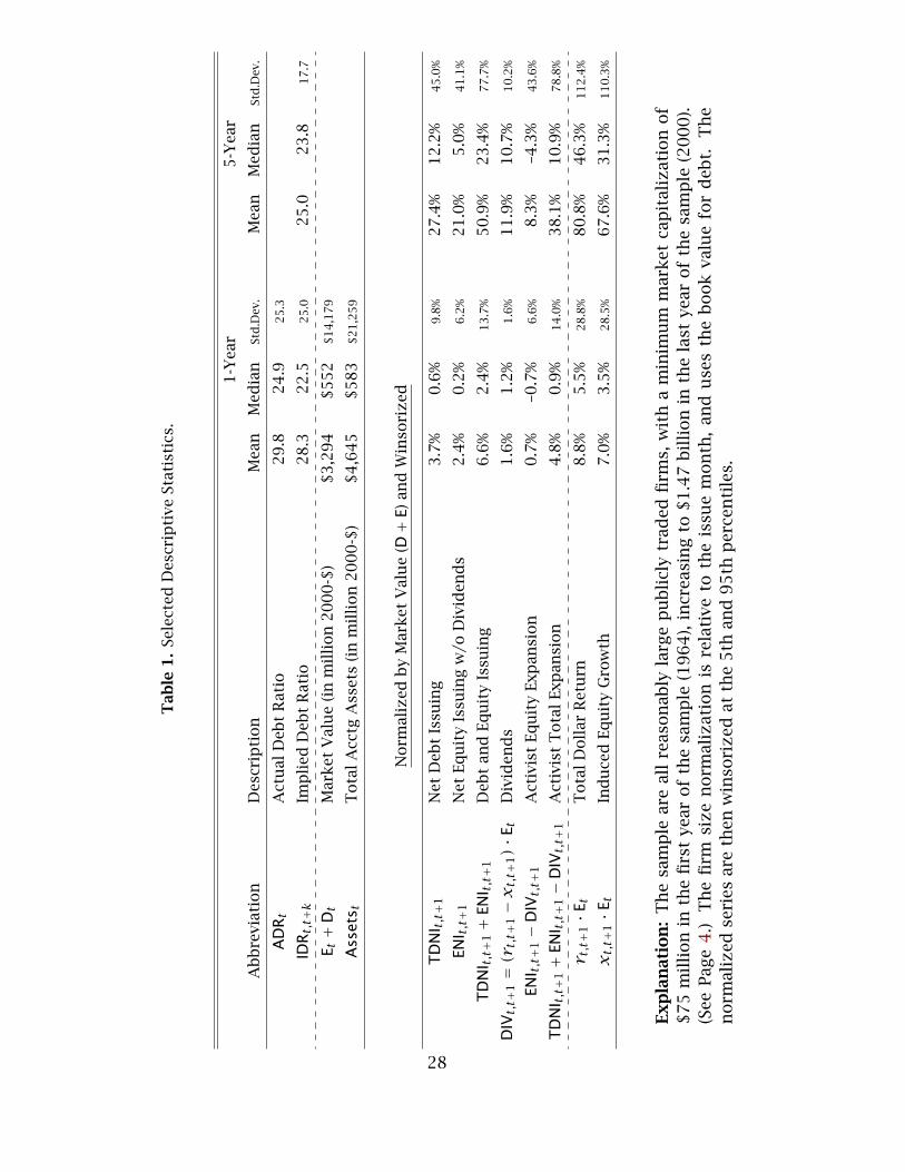
Insert Table 1 Here:Selected Descriptive Statistics.
Table 1 shows that the average sample firm is about $3.3 billion in market-value,
$4.6 billion in book value, both in 2000 dollars. However, the median firm is worth
only about $550 to $580 million. The debt ratio, the dependent variable, has a mean
of about 30% of firm value, and a median of about 25%.
A quick measure of the relative importance of the dynamic components of debt
ratios can be gleaned from summary statistics for the components of debt ratios,
normalized by firm size, Et +Dt in the month in which issues occur. Over 40 years,
corporations in the sample experience average stock return appreciations of 8.8%
(11.2% unwinsorized), of which they pay out 1.6% in dividends. Therefore, they
experience 7.0% (9.4% unwinsorized) in stock price induced capitalization change.
4

On average, firms also issue 3.7% in debt and 2.4% in equity. (All medians are below
their respective means.)
My paper investigates debt ratio dynamics primarily in cross-section. Dividends
show little cross-sectional dispersion (1.6%), which is why subsequent results are in-
different to running tests with stock returns (r ) or percent equity growths (x). Stock
induced equity growth heterogeneity (28.5%) is larger than managerial activity in-
duced heterogeneity (14.0%). However, contrary to a common academic perception
that issuing activity is rare, firms in the sample are not averse to issuing activity.
In both means and standard deviations, corporate net issuing activity is about half
as large as stock-market induced equity value changes. (And issuing activity is nec-
essarily larger than net issuing activity!) In principle, issuing activity may be large
enough to counteract a good part of the capital structure effects of stock returns.
Before estimating the full non-linear influence of stock returns, a simple clas-
sification can show the significance of stock returns. All firms are first sorted by
year, then by sales and, within each consecutive set of ten similarly sized firms, al-
located into ten bins based on their net stock return performance. This procedure
keeps a roughly equal number of firms in each decile, and maximizes the spread in
stock returns across decile, holding calendar year and firm size constant. The sort
itself does not use any historical capital structure information. The header rows in
Table 2 show the median net stock returns of each decile.
Insert Table 2 Here:Corporate Activity, Equity Growth, and Capital Structure, Classified by Stock Returns
(Year-Adjusted and Sales-Adjusted).
The first five data rows report corporate activity, the sixth row reports equity
growth, again all normalized by firm size in the month of activity. Over 1 year,
firms respond to poor performance with more debt issuing activity; and to good
performance with more equity issuing activity. This hints that firms do not im-
mediately readjust: firms whose debt ratios increase (decrease) due to poor (good)
stock return performance seem to use their issuing activities not to readjust, but
to amplify the stock return changes (see also Baker and Wurgler (2002)). However,
5
over both 1-year and 5-year horizons, the relationship is not strong. The fourth row
shows that the relationship between stock returns and “activist equity expansion”
is more U-shaped when dividends are considered.
The fifth row explores whether firms deliberately expand or contract in response
to stock price performance. Over annual horizons, the group average total firm
expansion is not only small, but also only a little more pronounced for firms expe-
riencing either very good or very bad stock returns. Over 5 year horizons, the very
best decile stock price performers do engage in some activist expansion, roughly
32% of their firm value (6% per year). Still, their five year stock return caused mech-
anistic equity growth is a much larger 265%. In other deciles, the activist expansion
is flat and economically small, ranging from 7% to 18%.
In sum, in cross-section, when compared to their direct influence on equity
growth, even large stock returns trigger only modest corporate activity. The me-
dian firm in each decile does not do much either to expand or contract the firm; or
to undo or amplify the effects of stock returns on debt ratios. Stock return based
sorts cannot uncover the large heterogeneity in issuing activity documented in Ta-
ble 1.
This paper is less interested in issuing activity per sé (e.g., as are Havakimian,
Opler and Titman (2001)), as it is in capital-structure relevant issuing activity. Not
all net issuing activity is equally important for corporate debt ratios. For example,
when a 100% equity financed firm issues equity, it does not change its debt ratio. Not
in the table, I sorted the subset of best stock performers (decile 10) by their debt-
equity ratios. Zero debt-equity firms were especially eager to issue more equity, a
median of 33% of firm value, which ultimately had no influence on capital structure.
The most levered quintile firms, where equity issues were most capital structure
relevant, issued only 9% in equity. Thus, the relatively high equity issuing activity
median of 16% in this tenth decile ends up not being as capital-structure relevant
as one might suspect.
The actual capital structure relevance of the dynamic components is explored
in the three lower rows. The “ending ADR” rows show that there is a large spread
6
of resulting debt ratios across firms having recently experienced different rates of
return. Over 1 year, firms that have underperformed the S&P500 by 55% end up with
an actual debt ratio of 37%, while firms that have outperformed the S&P500 by 79%
end up with an actual debt ratio of 14%. Over 5 years, the worst stock performers
end up with debt ratios of 41%, the best stock performers end up with debt ratios
of 13%.
The “starting ADR” rows show that the ending debt ratio differences are not
due to the originating debt ratios. Over 1 year horizons, starting leverage does not
correlate with net return performance: most return deciles start out with actual
debt ratios of just about 22%. Over 5 year horizons, if anything, firms with poorer
stock returns start out with lower debt ratios.
Any snapshot of actual debt ratios in the economy therefore reflects differences
in historical stock returns. Not in the table, when firms are sorted by ending debt
ratios instead of by stock returns (still year and sales adjusted), the lowest decile
median debt ratio firm (ADRt = 1%) has experienced +5% stock returns in the most
recent year (+53% in the most recent 5 years), while the highest decile median debt
ratio firm (ADRt = 75%) has experienced −13% (−19%) stock returns.
The “implied IDR” rows impute the effects of stock returns on starting debt
ratios (ADR) in the appropriate non-linear fashion (eq. 3). Can IDR explain future
debt ratios better than starting ADR? It appears so. In explaining ending ADR, the
implied debt ratio IDR fits visually better than the starting ADR. Of course, all power
of my later readjustment tests must derive from the extreme stock return deciles.
There is no economic difference between readjustment and non-readjustment for
firms that experience only small stock returns.
7
IV Estimation
A Regression Specification
Insert Table 3 Here:F-M Regressions explaining Future Actual Debt Ratios ADRt+k with Debt Ratios ADRt and
Stock-Return Modified Debt Ratios IDRt,t+k.
The basic regression specification of the paper, equation 1, is estimated in Ta-
ble 3. The reported coefficients and standard errors are computed from the time-
series of cross-sectional regression coefficients (called F-M, for Fama-Macbeth). Both
the methods and variables are discussed in detail in the Appendix, as is the robust-
ness to alternatives.
Panel A omits the intercept and thus does not allow for a constant debt ratio
target. Over annual horizons, the average firm shows no tendency to revert to its
old debt ratio, and instead allows its debt ratio to drift almost one-to-one (102.1%)
with stock returns. Over 5 to 10 years, firms began to readjust, but the influence of
stock returns through IDR remains more important than the effects of readjustment
activity.
Panel B shows that this ADR coefficient reflected less a desire of firms to revert
to their starting debt ratios, as a tendency of firms to prevent debt ratios from
wandering too far away from a constant: In competition with the constant, ADR
loses most economic significance.
I conclude that observed corporate debt ratios at any fixed point in time are
largely transient, comoving with stock returns. Any deliberate readjustment is slow
and modest.
8
B Change Regressions
The regression can also be estimated in changes and/or with a restriction that the
coefficients on IDR and ADR add up to 1:
ADRt+k = α0 + α1 · IDRt,t+k + (1−α1) · ADRt + εt (10)
Rearranging, the estimated regressions are
(ADRt+1 − ADRt) = 2.1% + 102.2% · (IDRt,t+1 − ADRt) R2 = 43.2% ;
(ADRt+5 − ADRt) = 8.0% + 92.9% · (IDRt,t+5 − ADRt) R2 = 40.2% .(11)
The coefficient estimates are highly statistically significant and a first difference
term in ADR adds no statistical or economic power. I can conclude that stock re-
turn induced equity changes have roughly a one-to-one influence on observed debt
ratio changes over 1 year horizons. Even over 5 year horizons, corporate debt ratio
reversion activity is rather modest.
C Variance Decomposition
One can isolate the dynamic components laid out in Equation 7. That is, it is possi-
ble to predict ADRt+k not only with ADRt updated only for stock returns (which is
IDRt,t+k), but also with ADRt updated, e.g., for corporate issuing activity between t
and t + k (keeping other dynamics components at a constant zero).
Insert Table 4 Here:Explanatory Power of Components of Debt Ratios and Debt Ratio Dynamics:
Time-Series Average R2’s from Cross-sectional F-M Regressions.
Table 4 shows that history is important: 85% of firms’ capital structure levels can
be explained by last year’s capital structures, 54% by capital structure 5 years earlier.
More interesting, the table also shows that stock-return induced changes in capital
structure are less important than corporate issuing activity, although not by much.
9

Over 1 year, stock returns1 are responsible for 43.2% of the change in debt ratios,
while all net issuing activities together are responsible for about 56.9% of the change
in debt ratios. Over 5 years, stock returns are responsible for 40.2% of debt ratio
changes, while all net issuing activities are responsible for 68.8%. (The two need not
add up to 100%.) In principle, there is more than enough capital structure relevant
corporate issuing activity to counteract stock-return induced equity growth. Firms
are not inactive: they just do not choose to counteract their stock returns.
But the conclusion that research should focus only on (capital structure relevant)
issuing activity would also be mistaken. If the ultimate goal is to explain capital
structure, explaining issuing activity alone cannot do the job—even if a researcher
could perfectly predict one-hundred percent of all managerial capital structure ac-
tivities, she would still miss close to half of the variation in year-to-year capital
structure changes. And, as Table 5 will show, one hundred percent is utopian.
Previously used variables have little power to explain any of this capital structure
relevant managerial activity.
Table 4 can also suggest where researchers should focus their efforts to better
explain debt ratios: debt issuing activities are more capital structure relevant than
equity issuing activities, even though Table 1 indicated equal heterogeneity. (Eq-
uity issuing presumably occurs more in firms already heavily equity-financed.) The
final rows narrow the culprit even further. Over both 1 year and 5 year horizons,
long-term debt issuing activities are most capital structure relevant.2 Over 5 year
horizons, equity issuing activities become as important as short-term debt issuing
activities, yet still only half as important as long-term debt issuing activity.
1Here, I mean IDR. Stock returns by themselves (without interaction with past capital structure)can explain only 26% of the 1-year change, and 15–25% of the 5-year change in ADR.
2Although Havakimian et al. (2001) seek to explain all, not just capital structure relevant, netissuing activity, they succeed only in explaining 1.8% of the variation in net long-term debt issuingactivities among 4,558 observations with large long-term debt changes.
10

D Aggregate Effects
The focus of this paper is the cross-section. Still, one can aggregate the debt and
market-equity of all firms on Compustat, and use the value-weighted market rate
of return to compute IDR. (The results are similar with only firms meeting the size
criterion.) The estimated single time-series regression on the aggregate data series
are
1-Year: ADRt+1 − ADRt = 2.3% + 105.9% · (IDRt,t+1 − ADRt) R2 = 89% ;
5-Year: ADRt+5 − ADRt = 11.2% + 93.3% · (IDRt,t+5 − ADRt−5) R2 = 82% .(12)
This suggests that the overall stock market level has a similarly long-lived effect on
the aggregate corporate debt ratio, just as it is the major influence in determining
the debt ratio of firms in cross-section. Unfortunately, the influence of stock returns
may be misstated here, because debt is quoted in terms of book value (for lack of
available market data); and, unlike in the cross-sectional year-by-year regressions, in
these regressions, annual aggregate interest rate changes can drive a considerable
wedge between book and market values of debt.
V Alternative Proxy Variables
A natural question is whether the variables used in the prior capital structure and
issuing literatures have economic relevance when the effects of stock returns are
properly controlled for. For example, corporate profitability was found to predict
lower debt ratios in previous studies. If profitability has no incremental significance
when IDR is controlled for, then it would have correlated with capital structures
only indirectly through its correlation with stock returns. Put differently, managers
would not so much have “acted” to lower their debt ratios (by issuing more net eq-
uity) when profitability increased. Instead, managers of more profitable companies
would have experienced higher stock prices, which in turn would have mechanisti-
cally reduced their debt ratios.
11
Insert Table 5 Here:F-M Regressions explaining Debt Ratio Changes (ADRt+k − ADRt).
Adding Variables Used in Prior Literature.
The multivariate columns in Table 5 estimate
ADRt+k − ADRt = α0 +α1 ·Xt,t+k +C∑c=1
[α2c · Vct +α2c+1 · Vct ×Xt,t+k
]+ ε , (13)
where Xt,t+k ≡ IDRt,t+k − ADRt, and V1 through VC are named third variables (de-
scribed in detail in the Appendix). When a coefficient on Vc is reliably positive, then
Vc incrementally helps to explain actual debt ratios. When a coefficient on Vc×Xt,t+kis positive, then Vc incrementally helps to explain readjustment. To avoid multi-
collinearity, the same specifications are also run with one Vc variable at a time in a
4-variate regression,
ADRt+k − ADRt = α0 +α1 ·Xt,t+k +α2 · Vct +α3 · Vct ×Xt,t+k + ε . (14)
The chosen Vc variables include most important variables used in prior capital struc-
ture and issuing literature. In contrast to existing literature, the Vc variables here
are challenged to explain not only issuing activity, but net issuing activity that is
capital-structure relevant and while in competition with IDR effects. Flow variables
are measured contemporaneously with the differencing interval in the dependent
variable. Thus, they are not known at the outset t, and some correlation will come
about if the proxy variable in later parts of the measuring period responds to debt
ratio changes in earlier parts of the measuring period, rather than vice-versa. This
is obviously not the case for stock returns. Thus, the reported power of the flow
variable coefficients is likely to be an optimistic estimate. (When flow variables are
measured strictly prior, they typically have zero influence.) The regressions in Ta-
ble 5 report unit-normalized coefficients (coefficient times standard deviation of the
variable in the sample). These coefficients indicate relative economic importance.
Over annual horizons, return-induced debt ratio changes have considerably big-
ger impact than do other proxies. A one-standard deviation higher ∆IDR is as-
socated with a 7.38% increase in debt ratio. (The non-standardized coefficient is
12
7.38%/0.07 ≈ 109.80%.) The best other proxy is that firms that have taken over
other firms also tend to increase leverage; and that firms that wander away from
their industry average debt/equity ratio seek to return to it. Asset-based Profitabil-
ity and Firm Volatility are statistically significant, but only of modest economic im-
portance. The only variable that suggests modestly greater non-adjustment (cross-
term) is asset-based profitability: More profitable firms tend to adjust less for stock
return induced capital structure changes.
Over five year horizons, return-induced debt ratio changes continue to exert the
strongest influence. (The non-standardized coefficient is 82%.) Again, the strong
negative coefficient on industry deviation suggests that firms are eager to move to-
wards their industry’s average debt ratio, and that firms that have engaged in M&A
activity tend to increase leverage. Two of the cross-coefficients indicate good eco-
nomic significance: firms with more profitable assets and firms with more volatility
tend to have avoided readjusting (but recall that return volatility is contempora-
neous with ∆IDR). Put differently, in a stratification, their ∆IDR coefficients in a
bivariate regression would be significantly higher than those of other firms.
The increase in R2, from the 43% in the 1-year difference regression when only
IDR is used, to the 54% reported R2 when the additional 20 variables in Table 5
are included is modest. The increase in R2 is a more pronounced for the 5-year
regressions (40% in the IDR-only regression, 59% in the 20+1 variable regression).
But it is fair to state that the additional 20 variables make only modest headway in
reducing the 60% variation that can be attributed to corporate net issuing activity.3
Most corporate issuing motives remain unexplained.
Some variables had to be excluded from Table 5, because data availability would
have dropped the number of observations in the multivariate specifications. In its
own 4-variate specification:
Graham’s Tax Rate is an improved iterative tax variable (Graham (2000)), which
over 5 years only works better than the simpler tax variable in Table 5. Firms
3A full set of 2-Digit SIC dummies raises the R2 by about 5%. Their inclusion does not changethe significance of most variables. Industry herding becomes a little more important, profitabilitya little less important.
13

with one-standard deviation higher tax rates are likely to take on an additional
2.4% in debt ratio over five years. Firms with higher tax rates are more likely
to non-adjust, and in an economically significant fashion.
Interest Coverage Firms with one standard deviation higher high cash flows rel-
ative to their interest payments reduced debt over 1 year, but only by 0.4
percent. However, the 5-year cross-variable was economically important, sug-
gesting that firms with more cash flows relative to their earnings readjust less,
not more.
(The most significant interest coverage related specification indicates that
firms with poor recent returns and very high interest payments are more likely
to unlever over the next year—perhaps necessary for survival.)
A number of other variables were found to be unimportant. Three variables are
interesting although/because they do not show any significance:
Uniqueness Sales-adjusted R&D and selling expenses (Titman and Wessels (1988))
have no incremental explanatory power over 1 year, and modest explanatory
power over 5 years. This is both due to the fact that high R&D firms had good
returns and due to the fact that many high R&D equity issuers are already
100% equity financed. (Such issues do not alter capital-structure.)
Future Stock Return Reversals Firms that experience large stock price reversals
the year after the measuring period do not behave differently from firms that
experience stock price continuation. Managers do not delay readjusting be-
cause they know something that the market does not know.
Profitability Changes Firms experiencing current profitability changes show no un-
usual capital structure activities or tendencies to change their debt ratios over
1 year, and very modest inclination over 5 years. Cross effects do not mat-
ter. This indicates that even firms whose stock returns and revised debt ratios
are due to or accompanied by immediate cash flow effects (rather than due to
long-run discount factor effects or due to far-off growth opportunities) are no
more eager to readjust.
14
In sum, although about half to two-thirds of the dynamics of capital structure
are due to net issuing activity, the variables here could not make a large dent in our
understanding of resulting capital structure. They could not explain much of the
part of capital structure that is not due to stock price changes. The proxies have only
modest incremental influence either in predicting higher debt ratios or in predicting
higher tendencies to readjust. Much of their correlation with capital structure in
earlier papers was due to their correlations with IDR, in many cases, a sufficient
statistic. None of these variables change the coefficient on the IDR variable, much
less rival it in importance.
VI Interpretation
Corporations are not inactive with respect to issuing activity. This makes it all the
more startling that they do not use their capital structure activities to counteract
the external and large influences of stock returns on their capital structures. The
challenge is to explain why. The answer must lie in the cost-benefit tradeoff to
undoing stock return induced capital structure changes. The benefits relate to how
the hypothetically friction-free optimal debt ratio shifts with stock returns. The
costs relate to direct financial transaction costs or indirect costs of change that can
arise from a variety of distortions.
1. Dynamic Optima: If the optimal debt ratio changes one-to-one with stock
returns, then there is no need for firms to rebalance towards their previous or static
debt ratio targets. For example, if stock prices relate more to changes in discount
factors and/or far-away growth opportunities, then firms with positive stock returns
would not experience changes in earnings in the near future. They may find that
increasing the debt ratio would provide few additional tax benefits in exchange
for risking a short-term liquidity crunch or outright bankruptcy (see also Barclay,
Morellec and Smith (2001)). Such theories can at least predict that stock returns
correlate negatively with debt ratios (over short horizons), the correct sign.
15

But, by itself, this explanation has drawbacks. First, the argument is less com-
pelling for Value Firms with already low debt ratios which experience further large
positive stock returns. (And a number of authors have argued that such firms al-
ready have too little debt.4) Such firms show no greater tendency to readjust or lever
up. Second, even firms experiencing the most immediate increases in profitability—
i.e., firms whose stock price movements are less likely due to far-away growth op-
portunities or discount rate changes—do not show any differences in their readjust-
ment tendencies. Third, it would be curious if the optimal dynamic debt ratio were
as one-to-one with stock-priced induced changes in equity values, as the evidence
suggests.
2. Direct Transaction Costs: This suggests that another part of the explanation
is likely to be transaction costs. Transaction costs cannot only induce path depen-
dency, but also produce flat corporate objective functions (Miller (1977), Fischer,
Heinkel and Zechner (1989), Leland (1998)). The fact that there is more readjust-
ment over longer horizons is also consistent with transaction costs playing a role.
But by itself, this explanation, too, has some drawbacks.
First, for large U.S. Corporations, direct transaction costs are small, and practi-
tioners believe them to be small (Graham and Harvey (2001)).
Second, readjustment patterns are similar across firms where transaction costs
are very different. Even if transaction costs are high for a firm that issues equity
to reduce debt in response to falling enterprise valuation,5 they are low for a firm
that issues debt to repurchase equity in response to increasing enterprise valuation.
Similarly, small firms should have higher transaction costs than large firms; and yet
Table 5 shows that large firms are no more eager to readjust. Finally, even firms
4The average (median) operating income divided by interest payments in the sample is 43 (6.5),suggesting only a modest probability of bankruptcy for many firms. An otherwise typical firm inthe sample ($500 million size, 33% tax rate, 25% debt ratio) that experiences a 5% debt-equity ratiochange should issue $40 million in debt, thus obtaining about 33% · $40 ≈ $13 million (perpetualNPV) in tax savings. Graham (2000) calculates that the average publicly traded firm could gainabout 10% in firm value if it increased its debt ratio.
5However, first a debt ratio can also be reduced by selling off assets to pay off debt or by usingformer dividends to repurchase debt. Second, equity values would have already fallen signifi-cantly, and an equity-for-debt exchange (e.g., with existing creditors) should increase enterprisevalue, not decrease it (absent direct frictions).
16

experiencing the most dramatic changes in debt ratios readjust very little, too. This
suggests that inventory-type transaction cost minimization models (under which
one should observe more readjustment for larger deviations from the optimum)
are not likely to explain the evidence.
Third, firms do not seem to lack the inclination to be capital structure active.
They just seem to lack the proper inclination to readjust for equity value changes!
(A more consistent transaction cost argument may have to suggest that transaction
costs are higher after large positive or negative equity movements.) And if corpora-
tions really wanted to readjust at low transaction costs, they could issue securities
that convert automatically into debt when corporate values increase and into equity
as corporate values decrease—the opposite of convertible securities. They do not.
3. Indirect Costs: A number of theories can explain why firms face implicit costs
to reacting or adjusting, either actual or perceived. These suffer from similar prob-
lems as direct transaction cost explanations: they can explain inertia better than
lack of readjustment, although firms are very active in real life, instead. Moreover,
few tests of such theories have explored their unique non-inertia implications.
The pecking order theory (Myers and Majluf (1984), Myers (1984)) is not the
only model of inertia, but it is the most prominent. Firms are reluctant to raise
more equity when their stock prices deteriorate because of negative inference by
investors. The theory is known to have more difficulties explaining why firms are
reluctant to rebalance more towards debt when their stock prices increase. To its
credit, the pecking order theory does not need to rely on an agency explanation
(debt discipline) to explain an additional fact, the negative stock price response to
equity issuing activity.
Other theories can predict corporate inertia if firms suffer from limited memory
retention (e.g., Hirshleifer and Welch (2002)); if agency or influence problems para-
lyze the firm (e.g., Rajan and Zingales (2000)); if managers believe that their equity
is too expensive/cheap for repurchases after stock price increases/decreases (e.g.,
Berger, Ofek and Yermack (1997)); if managers prefer equity to debt and increasing
equity values make them harder to dislodge (e.g., Zwiebel (1995)); or if firms en-
17

gage in near-rational or irrational behavior (e.g., Samuelson and Zeckhauser (1988),
Benartzi and Thaler (2001)).
Finally, one could argue that different reasons drive corporate behavior on the
upside and on the downside. For example, on the upside, managers may become
more entrenched and dislike issuing debt (or exchanging equity for debt); while on
the downside, managers may believe (or have inside information) that their firms
have become too “undervalued,” and dislike selling equity (or exchanging debt for
equity).
VII Prior Capital Structure Literature
My paper has shown that stock returns and stock return adjusted historical capital
structure are the best variables forecasting market-based capital structure.
Some prior literature has examined capital structure ratios not only based on
market equity value, but also book equity value. Yet, the book value of equity is
primarily a “plug number” to balance the LHS and RHS of the Balance Sheet—and it
can even be negative. Furthermore, book values correlate less with market values
among small firms. But more importantly, accounting rules imply that the book
value of equity increases with historical cash flows and decreases with asset depre-
ciation. Not surprisingly, profitability (growth) and fixed assets are the important
predictors of book-value based debt ratios (e.g., Shyam-Sunder and Myers (1999)).
Yet, some authors find book values attractive, because they have lower volatility
than market equity values, and therefore permit corporate issuing activity to ap-
pear more important.
In any case, compared to book value based debt ratios, interest coverage ratios
would be a much better alternative for measuring the advantages of debt to firms.
Operating cash flows (or cash) may be the best available measure of assets-in-place
and tax advantages. Immediate interest payments may be the best measure of po-
tential bankruptcy and liquidity problems. Thus, tradeoff theories may be better
tested with the ratio of current interest burden to current operating cash flows (or
18

cash). Moreover, managers are known to pay attention to coverage ratios, and credit
ratings (which are in turn highly related to coverage ratios). But before one sets one’s
hopes too high, the typical firm paid out only about 15% of its operating cash flows
in interest, indicating that most firms could probably have easily borrowed more.
My evidence of readjustment failure is in line with the survey responses in Gra-
ham and Harvey (2001): queried executives apparently care little about either trans-
action costs, or most theories of optimal capital structure, or rebalancing when eq-
uity values change. To the extent that they do care when actively issuing, managers
claim they care about financial flexibility and credit ratings for debt issues; and
about earnings dilution and past stock price appreciation for equity issues. Yet,
executives also claim that they issue equity to maintain a target debt-equity ratio,
especially if their firm is highly levered—for which we could not find much evidence.
Most existing empirical literature has interpreted capital structure from the per-
spective of proactive managerial choice. Titman and Wessels (1988) find that only
“uniqueness” (measured by R&D/sales, high selling expenses, and employees with
low quit rates) and earnings are reliably important. Rajan and Zingales (1995) offer
the definitive description of OECD capital structures and find a strong negative cor-
relation between market-book ratios and leverage. Like Rajan and Zingales, Barclay,
Smith and Watts (1995) find that debt ratios are negatively related to market/book
ratios. Graham (2003) surveys the voluminous tax literature. Havakimian et al.
(2001) find a mild tendency of firms to issue in order to return to a target debt-
equity accounting ratio. The implied debt ratio can subsume most of the variables
in this literature.
Baker and Wurgler (2002) investigate the influence of past stock market returns
(see also Rajan and Zingales (1995)). But they are interested in how these returns
influence the active issuing decisions of firms, and do not consider the implied
change. My own paper is more interested in the failure of firms to undo the effects
of stock returns, and the consequent strong relation between lagged stock returns
and capital structure. Other literature has focused on non-action, though none
has focused on the dramatic fluctuations that non-action can cause. In addition to
pecking order tests (such as Fama and French (2002) and Shyam-Sunder and Myers
19

(1999)), some theories have been built on transaction costs. For example, Fischer et
al. (1989) use option pricing theory and find that even small recapitalization costs
can lead to wide swings in optimal debt ratios.
Finally, some behavioral finance papers find similar lack of readjustment in other
contexts. For example, Thaler, Michaely and Benartzi (1997) find that, in contrast to
optimizing theories of dividend payments, managers seem to pay dividends more in
response to past earnings than in response to an expectation of future earnings. Be-
nartzi and Thaler (2001) find that “1/N” diversification heuristics are more powerful
than the effects of stock market value changes in pension portfolio adjustments.
VIII Conclusion
Market-based debt ratios describe the relative ownership of the firm by creditors and
equity holders, and they are an indispensable input in WACC computations. This
paper has shown that stock returns are a first order determinant of debt ratios;
that they are perhaps the only well understood influence of debt ratio dynamics;
and that many previously used proxies seem to have helped explain capital structure
dynamics primarily because they correlated with omitted dynamics caused by stock
price changes.
20
Appendix
A Method and Variable Details
A. Variable Definitions:
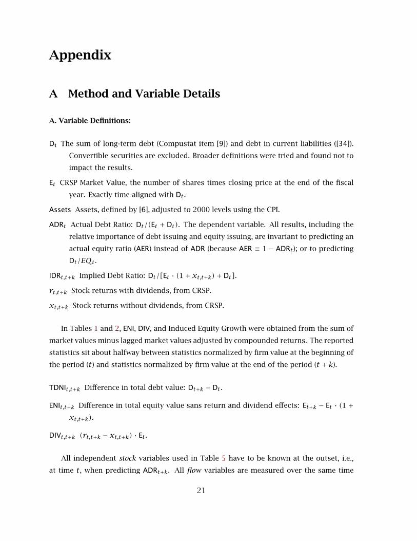
Dt The sum of long-term debt (Compustat item [9]) and debt in current liabilities ([34]).
Convertible securities are excluded. Broader definitions were tried and found not to
impact the results.
Et CRSP Market Value, the number of shares times closing price at the end of the fiscal
year. Exactly time-aligned with Dt .
Assets Assets, defined by [6], adjusted to 2000 levels using the CPI.
ADRt Actual Debt Ratio: Dt/(Et + Dt). The dependent variable. All results, including the
relative importance of debt issuing and equity issuing, are invariant to predicting an
actual equity ratio (AER) instead of ADR (because AER ≡ 1 − ADRt); or to predicting
Dt/EQt .
IDRt,t+k Implied Debt Ratio: Dt/[Et · (1+ xt,t+k)+Dt].
rt,t+k Stock returns with dividends, from CRSP.
xt,t+k Stock returns without dividends, from CRSP.
In Tables 1 and 2, ENI, DIV, and Induced Equity Growth were obtained from the sum of
market values minus lagged market values adjusted by compounded returns. The reported
statistics sit about halfway between statistics normalized by firm value at the beginning of
the period (t) and statistics normalized by firm value at the end of the period (t + k).
TDNIt,t+k Difference in total debt value: Dt+k −Dt .
ENIt,t+k Difference in total equity value sans return and dividend effects: Et+k − Et · (1 +xt,t+k).
DIVt,t+k (rt,t+k − xt,t+k) · Et .
All independent stock variables used in Table 5 have to be known at the outset, i.e.,
at time t, when predicting ADRt+k. All flow variables are measured over the same time
21

interval as the rate of return, i.e., from t to t + k. (Over 5 years, the reported SDV’s are for
the average over the 5 flow variables, not the sum.)
Tax Rate Total Income Tax ([16]), divided by the sum of Earnings ([53]×[54]) plus Income
Tax ([16]). Winsorized to between −100% and +200%.
Log Equity Volatility Standard deviation of returns, computed from CRSP. Timed from
t − 1 to t. Logged, not winsorized.
Log Firm Volatility Equity Volatility times Et/(Et +Dt). Logged, not winsorized.
M&A Activity A dummy of 1 if Compustat footnotes indicate a flag of AA, AR, AS, FA, FB,
FC, AB, FD, FE, or FF.
Profitability, Sales Operating Income ([13]) divided by Sales ([12]). Winsorized at 5% and
95%.
Profitability, Assets Operating Income ([13]) divided by Assets ([6]). Winsorized at 5% and
95%.
Stock Returns As used in the IDR computation, but by itself.
Book/Market Ratio Book Value of Equity ([60]) divided by CRSP Market Value. Winsorized
at 5% and 95%.
Log Assets See Assets. Not winsorized.
Log Rel. Mkt. Cap. E divided by the price level of the S&P500. Always greater than 0.1.
Deviation from Industry Debt Ratio (Industry herding or conformity.) ADR of a firm mi-
nus the ADR average in its three-digit SIC code industry. (Similar answers are ob-
tained if two-digit industry definitions are used instead.) This variable was also used
in Havakimian et al. (2001). MacKay and Philips (2002) independently provide a
more detailed examination of industry capital structure. Bikhchandani, Hirshleifer
and Welch (1998) review the herding literature.
Independent variables described in the text following Table 5:
Selling Expense Selling Expense ([189]) divided by Sales ([12]). Winsorized at 5% and 95%.
R&D Expense R&D Expense ([46]) divided by Sales ([12]). Winsorized at 5% and 95%.
Interest Coverage Operating Income ([13]) divided by Interest Paid ([15]). Winsorized at
5% and 95%.
Graham’s Tax Rate Provided by John Graham. See Graham (2000).
22

Future Stock Return Reversals This variable is not fully known at time t. It multiplies the
stock returns from t, t + k with stock returns from t + k, t + 2k. Thus, the variable
measures “future price continuation” (consecutive positive and consecutive negative
rates of return result in positive values). Not winsorized.
Profitability Changes This variable is not fully known at time t. Profitability divided by
sales, an average from t to t + k, minus Profitability divided by sales at t − 2. Other
definitions were tried, and not found to make a difference. Not winsorized.
In some cases, various variable definitions were explored. The results were robust, in that
no reported insignificant variable achieved significance in alternatives, and vica-versa.
B. Fama-Macbeth Method: Regressions in Tables 3, 4, and 5 are run one Compustat pe-
riod at a time. (In Compustat, year 1987 includes firms with fiscal years ending between
June 1987 and May 1988). The coefficients and standard errors reported in the tables are
computed from the time-series of OLS regression coefficients. (Cross-sectional standard
errors are therefore ignored.) In general, the reader is well advised to ignore statistical
standard errors. Statistical significance at conventional significance levels is rarely lack-
ing. The reader’s first concern should be the economic meaning of the coefficients, not
their statistical significance.
Pooling all firm-years (instead of F-M) does not change coefficient estimates: for exam-
ple, a 1-year pooled regressions has coefficients of 2.7%, 101.7%, and –5.9%, instead of the
reported 2.7%, 101.4%, and –5.3% coefficients in the F-M method. Fixed-effects regressions
keep the IDR coefficient at about the same level, but drop the ADR coefficient, in some cases
to –30%.
When horizons are more than 1 year, the same firm can appear in overlapping regres-
sions. Overlap does not change the coefficient estimates: for example, in a 10-year regres-
sion that is run with three non-overlapping periods (1970–1980; 1980–1990; 1990-2000),
the coefficient estimates are 13.9%, 75.1%, and 6.0%, instead of the reported 13.8%, 70.8%,
and 6.9% coefficients in the paper. Statistical significance drops mildly, but no reported
inference in this paper changes.
Not reported, the F-M coefficient estimates typically have negative serial correlation.
For example, the coefficient time-series of IDR in the annual regressions displays a nega-
tive serial correlation of about −50%, which implies that the critical 5% level is around 1.1,
not 1.96. This negative serial correlation in coefficients implies that the standard errors
23

are overstated. However, although for the 1-year levels regressions, the firm-specific resid-
uals from the cross-sectional regressions also have on average a negative −12% time-series
correlation (from regression to regression), this is not the case for the differences regres-
sion (+30% correlation). The rolling overlap in the 5-year regressions further increases the
same-firm residual correlation (to +42%). This average positive serial correlation in resid-
uals implies that the standard errors are understated. Fortunately, even if one increases
the standard error by a factor of√T = 37 ≈ 6 (i.e., a worst case) or used the average cross-
sectional standard error instead of the time-series variation in the F-M coefficients, the
inferences in Table 3 would not change. And in Table 5, it is the economic significance of
the variable coefficients that is emphasized, anyway.
The residuals in cross-sectional or pooled regressions have a nice bell shape and are
generally well behaved. In cross-sectional regressions, unit-roots are not a concern (even
if the autocoefficient is close to 1).
C. Other Robustness Checks
Reported results in Table 2 are robust with respect to the use of means rather than
medians (or vica-versa). All results are robust with respect to the use of various scale
controls; and with respect to different definitions of debt, specifically to the use of short-
term and investment grade debt only (so that the debt is almost risk-free, which eliminates
much concern about the use of debt book value rather than the debt market value).
Unfortunately, the more interesting hypothesis that firms target an optimal debt ratio
(rather than just their past debt ratio) is not explorable due to lack of identification of an
“optimum”—both theoretically and empirically. However, added lags in actual debt ratio
terms in the regressions have no significance.
Over longer horizons, there are fewer observations because firms can disappear. Pre-
dicting debt ratios in 2000, the 10-year regression predicts debt ratios for only 1,131 firms,
while the equivalent 1-year regression has 2,679 firms. To my surprise, simulations indicate
that survivorship bias does not significantly influence the ADR/IDR coefficient estimates.
Even eliminating all firms with negative stock returns barely budges the coefficient esti-
mates. (The better stock performance of more levered companies in Table 2 is probably
influenced by survivorship bias.)
The robustness of the specifications in Table 5 was confirmed with alternatives in
which either the plain or the crossed variable were included only by themselves. Fur-
24

ther, the lack of cross-sectional predictability in readjustment tendency (the cross-term)
also clearly shows up when we use each variable to classify observations into quintiles,
and compare the IDR/ADR coefficients across quintiles. The estimated coefficients on IDR
are always close to 1 in all quintile subcategories and not very different from one another.
The one exception is M&A activity in the latter half of the sample period: in a classification
table, acquirors do show systematic debt increases (relative to the stock return implied
debt ratios). In sum, the modest significance in any of the cross-variables indicates that
non-readjustment is a relatively universal phenomenon, at least across the examined di-
mensions.
References
Baker, Malcolm and Jeffrey Wurgler. “Market Timing And Capital Structure.” The Journal of Finance
57-1 (February 2002): 1–32.
Barclay, Michael J., Clifford W. Smith, and Ross L. Watts. “The Determinants Of Corporate Leverage
And Dividend Policies.” Journal of Applied Corporate Finance 7-4 (Winter 1995): 4–19.
, Erwan Morellec, and Clifford W. Smith. “On the Debt Capacity of Growth Options.”
Manuscript. Rochester: University of Rochester, Simon School, June 2001.
Benartzi, Shlomo and Richard Thaler. “Naive Diversification Strategies In Retirement Saving Plans.”
American Economic Review 91-1 (March 2001): 79–98.
Berger, Philip G., Eli Ofek, and David L. Yermack. “Managerial Entrenchment and Capital Structure
Decisions.” The Journal of Finance 52-4 (September 1997): 1411–1438.
Bikhchandani, Sushil, David Hirshleifer, and Ivo Welch. “Learning from the Behavior of others: Con-
formity, Fads, and Informational Cascades.” Journal of Economic Perspectives 12-3 (Summer
1998): 151–170.
Fama, Eugene F. and Kenneth R. French. “Testing Trade-off and Pecking Order Predictions About
Dividends and Debt.” Review of Financial Studies 15-1 (Spring 2002): 1–34.
Fischer, Edwin O., Robert Heinkel, and Josef Zechner. “Dynamic Capital Structure Choice: Theory
And Tests.” The Journal of Finance 44-1 (March 1989): 19–40.
Graham, John R. “How Big Are The Tax Benefits Of Debt?” The Journal of Finance 55-5 (December
2000): 1901–1941.
25

. “Taxes and Corporate Finance: A Review.” Review of Financial Studies ( 2003): p. forthcoming.
and Campbell Harvey. “The Theory And Practice Of Corporate Finance: Evidence From The
Field.” Journal of Financial Economics 60 (May 2001): 187–243.
Havakimian, Armen, Timothy C. Opler, and Sheridan Titman. “The Debt-Equity Choice: An Analysis
Of Issuing Firms.” Journal of Financial and Quantitative Analysis 36-1 (March 2001): 1–24.
Hirshleifer, David and Ivo Welch. “An Economic Approach To The Psychology Of Change: Amnesia,
Inertia, And Impulsiveness.” Journal of Economics and Management Strategy 11-3 (Fall 2002):
379–421.
Leland, Hayne E. “Agency Costs, Risk Management, And Capital Structure.” The Journal of Finance
49 (August 1998): 1213–1252.
MacKay, Peter and Gordon M. Philips. “Is There an Optimal Industry Financial Structure?”
Manuscript: University of Maryland, April 2002.
Miller, Merton H. “Debt and Taxes.” The Journal of Finance 32-2 (May 1977): 261–275.
Myers, Steward C. “The Capital Structure Puzzle.” The Journal of Finance 39-4 (July 1984): 575–592.
Myers, Stewart C. and Nicholas S. Majluf. “Corporate Financing and Investment Decisions when
Firms Have Information that Investors do not Have.” Journal of Financial Economics 13-2
(June 1984): 187–221.
Rajan, Raghuram G. and Luigi Zingales. “What Do We Know About Capital Structure: Some Evidence
From International Data.” The Journal of Finance 50-5 (December 1995): 1421–1460.
and . “The Tyranny of Inequality: An Inquiry into the Adverse Consequences of Power
Struggles?” Journal of Public Economics 76 (June 2000): 521–558.
Samuelson, William and Richard J. Zeckhauser. “Status Quo Bias in Decision Making.” Journal of
Risk and Uncertainty 1 (March 1988): 7–59.
Shyam-Sunder, Lakshmi and Steward C. Myers. “Testing static tradeoff against pecking order mod-
els of capital structure.” Journal of Financial Economics 51-2 (February 1999): 219–243.
Thaler, Richard H., Roni Michaely, and Shlomo Benartzi. “Do Changes In Dividends Signal The
Future Or The Past?” The Journal of Finance 52-3 (July 1997): 1007–34.
Titman, Sheridan and Roberto Wessels. “The Determinants Of Capital Structure.” The Journal of
Finance 43-3 (March 1988): 1–19.
26

Zwiebel, Jeffrey. “Corporate Conservatism, Herd Behavior And Relative Compensation.” Journal of
Political Economy 103-1 (February 1995): 1–25.
B Tables
Editor: If dashed lines are not available, please replace dashed lines with extra space for visualseparation, not with solid lines.
27
Tab
le1
.Se
lect
edD
escr
ipti
veSt
atis
tics
.
1-Y
ear
5-Y
ear
Ab
bre
viat
ion
Des
crip
tio
nM
ean
Med
ian
Std
.Dev
.M
ean
Med
ian
Std
.Dev
.
AD
Rt
Act
ual
Deb
tR
atio
29
.82
4.9
25
.3
IDRt,t+k
Imp
lied
Deb
tR
atio
28
.32
2.5
25
.02
5.0
23
.81
7.7
E t+
Dt
Mar
ket
Val
ue
(in
mil
lio
n2
00
0-$
)$
3,2
94
$5
52
$1
4,1
79
Ass
ets t
To
tal
Acc
tgA
sset
s(i
nm
illi
on
20
00
-$)
$4
,64
5$
58
3$
21
,25
9
No
rmal
ized
by
Mar
ket
Val
ue
(D+
E)an
dW
inso
riz
ed
TD
NI t,t+
1N
etD
ebt
Issu
ing
3.7
%0
.6%
9.8
%2
7.4
%1
2.2
%4
5.0
%
ENI t,t+
1N
etEq
uit
yIs
suin
gw
/oD
ivid
end
s2
.4%
0.2
%6
.2%
21
.0%
5.0
%4
1.1
%
TD
NI t,t+
1+
ENI t,t+
1D
ebt
and
Equ
ity
Issu
ing
6.6
%2
.4%
13
.7%
50
.9%
23
.4%
77
.7%
DIVt,t+
1=(rt,t+
1−xt,t+
1)·E
tD
ivid
end
s1
.6%
1.2
%1
.6%
11
.9%
10
.7%
10
.2%
ENI t,t+
1−
DIVt,t+
1A
ctiv
ist
Equ
ity
Exp
ansi
on
0.7
%–0
.7%
6.6
%8
.3%
–4.3
%4
3.6
%
TD
NI t,t+
1+
ENI t,t+
1−
DIVt,t+
1A
ctiv
ist
To
tal
Exp
ansi
on
4.8
%0
.9%
14
.0%
38
.1%
10
.9%
78
.8%
r t,t+
1·E
tT
ota
lD
oll
arR
etu
rn8
.8%
5.5
%2
8.8
%8
0.8
%4
6.3
%1
12
.4%
xt,t+
1·E
tIn
du
ced
Equ
ity
Gro
wth
7.0
%3
.5%
28
.5%
67
.6%
31
.3%
11
0.3
%
Ex
pla
nat
ion
:T
he
sam
ple
are
all
reas
on
ably
larg
ep
ub
licl
ytr
aded
firm
s,w
ith
am
inim
um
mar
ket
cap
ital
izat
ion
of
$7
5m
illi
on
inth
efi
rst
year
of
the
sam
ple
(19
64
),in
crea
sin
gto
$1
.47
bil
lio
nin
the
last
year
of
the
sam
ple
(20
00
).(S
eePa
ge4
.)T
he
firm
siz
en
orm
aliz
atio
nis
rela
tive
toth
eis
sue
mo
nth
,an
du
ses
the
bo
ok
valu
efo
rd
ebt.
Th
en
orm
aliz
edse
ries
are
then
win
sori
zed
atth
e5
than
d9
5th
per
cen
tile
s.
28
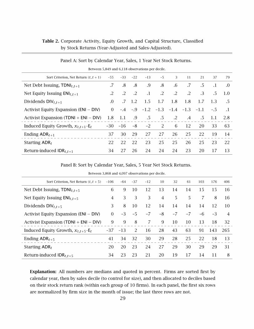
Table 2. Corporate Activity, Equity Growth, and Capital Structure, Classified
by Stock Returns (Year-Adjusted and Sales-Adjusted).
Panel A: Sort by Calendar Year, Sales, 1 Year Net Stock Returns.
Between 5,849 and 6,118 observations per decile.
Sort Criterion, Net Return (t, t + 1) –55 –33 –22 –13 –5 3 11 21 37 79
Net Debt Issuing, TDNIt,t+1 .7 .8 .8 .9 .8 .6 .7 .5 .1 .0
Net Equity Issuing ENIt,t+1 .2 .2 .2 .1 .2 .2 .2 .3 .5 1.0
Dividends DIVt,t+1 .0 .7 1.2 1.5 1.7 1.8 1.8 1.7 1.3 .5
Activist Equity Expansion (ENI−DIV) 0 –.4 –.9 –1.2 –1.3 –1.4 –1.3 –1.1 –.5 .1
Activist Expansion (TDNI+ ENI−DIV) 1.8 1.1 .9 .5 .5 .2 .4 .5 1.1 2.8
Induced Equity Growth, xt,t+1·Et –30 –16 –8 –2 2 6 12 20 33 63
Ending ADRt+1 37 30 29 27 27 26 25 22 19 14
Starting ADRt 22 22 22 23 25 25 26 25 23 22
Return-induced IDRt,t+1 34 27 26 24 24 24 23 20 17 13
Panel B: Sort by Calendar Year, Sales, 5 Year Net Stock Returns.
Between 3,868 and 4,097 observations per decile.
Sort Criterion, Net Return (t, t + 5) –106 –64 –37 –12 10 32 61 103 176 406
Net Debt Issuing, TDNIt,t+5 6 9 10 12 13 14 14 15 15 16
Net Equity Issuing ENIt,t+5 4 3 3 3 4 5 5 7 8 16
Dividends DIVt,t+5 3 8 10 12 14 14 14 14 12 10
Activist Equity Expansion (ENI−DIV) 0 –3 –5 –7 –8 –7 –7 –6 –3 4
Activist Expansion (TDNI+ ENI−DIV) 9 9 8 7 9 10 10 13 18 32
Induced Equity Growth, xt,t+5·Et –37 –13 2 16 28 43 63 91 143 265
Ending ADRt+5 41 34 32 30 29 28 25 22 18 13
Starting ADRt 20 20 23 24 27 29 30 29 29 31
Return-induced IDRt,t+5 34 23 23 21 20 19 17 14 11 8
Explanation: All numbers are medians and quoted in percent. Firms are sorted first by
calendar year, then by sales decile (to control for size), and then allocated to deciles based
on their stock return rank (within each group of 10 firms). In each panel, the first six rows
are normalized by firm size in the month of issue; the last three rows are not.
29

Table 3. F-M Regressions explaining Future Actual Debt Ratios ADRt+k withDebt Ratios ADRt and Stock-Return Modified Debt Ratios IDRt,t+k.
Panel A: Without Intercept.
Horizon k con. IDRt,t+k ADRt s.e.c s.e.IDR s.e.ADR R2 T
1-Year F-M 102.1 –0.5 1.4 1.4 96.3% 37
3-Year F-M 94.6 9.5 2.1 2.1 90.4% 35
5-Year F-M 86.7 18.7 2.8 2.1 86.5% 33
10-Year F-M 68.3 37.7 4.6 1.8 80.0% 28
Panel B: With Intercept.
Horizon k con. IDRt,t+k ADRt s.e.c s.e.IDR s.e.ADR R2 T
1-Year F-M 2.7 101.4 –5.3 0.1 1.3 1.2 91.3% 37
3-Year F-M 6.8 94.4 –4.2 0.3 1.5 1.4 78.4% 35
5-Year F-M 9.3 86.9 –0.5 0.4 2.1 1.6 70.2% 33
10-Year F-M 13.8 70.8 +6.9 0.6 3.7 2.7 56.0% 28
Explanation: The cross-sectional regression specifications are
ADRt+k = [α0+] α1 · IDRt,t+k +α2 · ADRt + εt+k .
Reported coefficients and standard error estimates are computed from the time-series of cross-sectional regression coefficients, and quoted in percent. A coefficientof 100% on implied debt ratio (IDRt,t+k) indicates perfect lack of readjustment, acoefficient of 100% on actual debt ratio (ADRt) indicates perfect readjustment. R2’sare time-series averages of cross-sectional estimates. 60,317 firm-years are usedin the 1-year regressions, 25,180 in the 10-year regressions. T is the number ofcross-sectional regressions.
30

Tab
le4
.Ex
pla
nat
ory
Pow
ero
fC
om
po
nen
tso
fD
ebt
Rat
ios
and
Deb
tR
atio
Dyn
amic
s:T
ime-
Seri
esA
vera
geR
2’s
fro
mC
ross
-sec
tio
nal
F-M
Reg
ress
ion
s.
k=
1-Y
ear,
AvgR
2k=
5-Y
ears
,AvgR
2
InLe
vels
,AD
Rt+k
isex
pla
ined
by
Reg
ress
or
(th
isco
lum
n).
InD
iffer
ence
s,A
DRt+k−
AD
Rt
isex
pla
ined
by
Reg
ress
or
Min
us
AD
Rt.
Leve
lsD
iffer
-en
ces
Leve
lsD
iffer
-en
ces
Past
Deb
tR
atio
,AD
Rt
Dt
Dt+
E t8
5.0
%5
4.0
%
Imp
lied
Deb
tR
atio
,ID
Rt,t+k
Dt
Dt+
E t·(
1+xt,t+k)
91
.2%
43
.2%
68
.3%
40
.2%
Imp
lied
Deb
tR
atio
,w/
div
iden
dp
ayo
ut
Dt
Dt+
E t·(
1+r t,t+k)
91
.3%
43
.6%
70
.0%
41
.5%
All
issu
ing
and
div
iden
dac
tivi
tyDt+
TD
NI t,t+k
Dt+
TD
NI t,t+k+
E t+
ENI t,t+k−
DIVt,t+k
93
.4%
56
.9%
85
.7%
68
.8%
All
issu
ing
acti
vity
Dt+
TD
NI t,t+k
Dt+
TD
NI t,t+k+
E t+
ENI t,t+k
93
.4%
56
.5%
84
.9%
65
.9%
Net
Equ
ity
Issu
ing
Act
ivit
yDt
Dt+
E t+
ENI t,t+k−
DIVt,t+k
85
.6%
5.2
%6
3.3
%1
6.2
%
Net
Deb
tIs
suin
gA
ctiv
ity
Dt+
TD
NI t,t+k
Dt+
TD
NI t,t+k+
E t9
2.3
%4
9.7
%7
1.3
%4
0.6
%
—"
—C
on
vert
ible
sO
nly
3.3
%4
.0%
—"
—Sh
ort
-Ter
mO
nly
15
.9%
13
.7%
—"
—Lo
ng-
Ter
mO
nly
30
.7%
31
.9%
31

Table 5. F-M Regressions explaining Debt Ratio Changes (ADRt+k − ADRt).Adding Variables Used in Prior Literature.
k = 1-Year k = 5-year
Variable Multivariate 4-Variate SDV Multivariate 4-Variate SDV
Intercept 2.70*
varies −0.62 varies
(Flow Variables Measured from t to t + k)∆IDR≡ IDRt,t+k − ADRt 7.38
***varies 0.07 10.47
**varies 0.13
Log Volatility −2.54*** −0.61
***0.80 −5.27
*** −0.30 0.67
— ×∆IDR − 0.97 −0.18 0.19 3.33 3.83*
0.37
Stock Return −0.06 −0.28 0.54 −1.33 −1.68 3.78
— ×∆IDR −0.46 0.32 0.08 −3.02* −0.79 1.12
M&A Activity 1.26***
1.28***
0.39 2.51***
2.17***
0.24
— ×∆IDR 0.08 0.06 0.03 0.34 −0.07 0.04
Profitability, Sales −0.20 −0.09 0.14 −1.29*** −0.17 0.12
— ×∆IDR −0.40 0.01 0.01 −0.97* −0.39 0.03
Profitability, Assets −1.45*** −0.62
***0.09 −2.57
*** −0.40 0.08
— ×∆IDR 0.91***
0.74***
0.01 1.76**
3.19***
0.02
Tax Rate 0.25* −0.05 0.28 0.74
***0.73
*0.17
— ×∆IDR −0.03 0.22 0.03 0.19 1.75***
0.05
(Stock Variables Measured at t)
Industry Deviation −1.83*** −1.13
***0.19 −6.87
*** −4.86***
0.21
— ×∆IDR −0.14 −0.14 0.01 −0.91* −0.73 0.03
Log Assets −2.71*** −0.20
*1.88 −4.67
*** −0.58**
1.93
— ×∆IDR −2.62 0.22 0.44 1.42 −1.49 0.84
Log Rel Mkt Cap 1.77***
0.01 1.54 3.47***
0.54 1.71
— ×∆IDR 0.75 0.12 0.10 0.53 −0.07 0.26
Book/Market Ratio 0.16 −0.22 0.55 0.75* −1.19
***0.57
— ×∆IDR 0.37 0.24 0.07 0.61 −0.02 0.17
N,T 57,921, 37 varies 34,880, 33 varies
R2 54% varies 59% varies
Explanation: The reported coefficient estimates are computed from the time-series of cross-sectional regression coefficients, and quoted in percent. Except for the intercept, variables wereunit-normalized (coefficients were multiplied by SDV, the standard deviation of the variable).One/two/three stars means a F-M-type t-statistic above 3/4/5. The multivariate columns are thecoefficients from one big specification. The 4-Variate columns are the coefficients from individualspecifications, one variable V at a time, ADRt+k−ADRt = α0+α1·Xt,t+k+α2·V+α3·V×Xt,t+k+εt+k.4-Variate regressions avoid multicollinearity.
32
Top Related