


Languages
Pages
Legal


Cambridge-INET Working Paper Series No: 2020/24
Cambridge Working Papers in Economics: 2041
WHEN IS THE FISCAL MULTIPLIER HIGH?
A COMPARISON OF FOUR BUSINESS CYCLE PHASES
Travis Berge Maarten De Ridder Damjan Pfajfar (Federal Reserve Board) (University of Cambridge) (Federal Reserve Board)
This paper compares the effect of fiscal spending on economic activity across four phases of the business cycle. We show that the fiscal multiplier is higher when unemployment is increasing than when it is decreasing. Conversely, fiscal multipliers do not depend on whether the unemployment rate is above or below its long-term trend. This result emerges both in the analysis of long time-series at the U.S. national level as well as for a post-Vietnam War panel of U.S. states. Our findings synthesize previous, at times conflicting, evidence on the state-dependence of fiscal multipliers and imply that fiscal intervention early on in economic downturns is most effective at stabilizing output. JEL: E62; C31; C32 Keywords: Fiscal multipliers; countercyclical policy; cross-sectional analysis; local projections
Cambridge-INET Institute
Faculty of Economics
When is the Fiscal Multiplier High?A Comparison of Four Business Cycle Phases*
Travis Berge†
Federal Reserve BoardMaarten De Ridder‡
University of CambridgeDamjan Pfajfar§
Federal Reserve Board
April 25, 2020
Abstract
This paper compares the effect of fiscal spending on economic activity across four phases ofthe business cycle. We show that the fiscal multiplier is higher when unemployment is in-creasing than when it is decreasing. Conversely, fiscal multipliers do not depend on whetherthe unemployment rate is above or below its long-term trend. This result emerges both inthe analysis of long time-series at the U.S. national level as well as for a post-Vietnam Warpanel of U.S. states. Our findings synthesize previous, at times conflicting, evidence on thestate-dependence of fiscal multipliers and imply that fiscal intervention early on in economicdownturns is most effective at stabilizing output.
Keywords: Fiscal multipliers; countercyclical policy; cross-sectional analysis; local projections
JEL classification: E62; C31; C32.
*The views expressed in this paper are those of the authors and do not necessarily reflect those of the Federal Reserve Board.†Address: Board of Governors of the Federal Reserve System, 20th and Constitution Ave NW, Washington, DC 20551, U.S.A.
E-mail: [email protected]. Web: https://www.federalreserve.gov/econres/travis-j-berge.htm.‡Address: University of Cambridge, Faculty of Economics, Sidgwick Ave, Cambridge, CB3 9DD, U.K. E-mail:
[email protected]: http://www.maartenderidder.com/.§Address: Board of Governors of the Federal Reserve System, 20th and Constitution Ave NW, Washington, DC 20551, U.S.A.
E-mail: [email protected]. Web: https://sites.google.com/site/dpfajfar/.
1

1 Introduction
Fiscal policy is frequently used to stabilize macroeconomic fluctuations. By implementing expansion-
ary policies during downturns and contractionary policies during upturns, policymakers aim to reduce
variation in economic activity and (un)employment. The effectiveness of such countercyclical policies
remains the subject of debate. In particular, there is a wide variety of views on the magnitude and cycli-
cal properties of the ‘fiscal multiplier’, which measures the increase in output from a given increase in
government spending. If the multiplier exceeds one, an increase in spending stimulates private spending
and raises output beyond the government’s initial expense. Conversely, a multiplier below one implies
that government spending crowds out private spending and is therefore less effective at stimulating ac-
tivity. Research in the aftermath of the Great Recession, spurred by contractionary policies in Europe,
suggests that the size of the multiplier depends on the state of the economy, and often exceeds unity dur-
ing recessions (Auerbach and Gorodnichenko 2012b, Blanchard and Leigh 2013, Nakamura and Steinsson
2014). A high recession-multiplier implies that well-timed fiscal policy can spur economic growth even
if the multiplier is lower than one on average over the business cycle. Recent evidence from an extended
historical analysis, however, suggests that multipliers are below one and do not vary over the business
cycle (Ramey and Zubairy 2018). That would limit the scope for countercyclical fiscal policy. A reconcili-
ation of these results is needed to allow for future assessments of the benefits of fiscal stimulus.
This paper shows that the effect of fiscal spending on output does depend on the state of the economy.
Specifically, we show that fiscal multipliers are higher when the unemployment rate is increasing than
when it is decreasing. Our estimated multipliers are furthermore larger than one when unemployment is
increasing in almost all specifications. In line with Ramey and Zubairy (2018), we do not find higher fiscal
multipliers when the unemployment rate is above its trend compared to when the unemployment rate is
below its trend. To obtain these results we deploy two established approaches from the literature on fiscal
spending and economic activity. We aim to show that existing measures of fiscal multipliers share the
prediction that multipliers are higher when unemployment is rising. We first assess the cyclical properties
of fiscal multipliers in the historical data from 1889 to 2015 from Ramey and Zubairy (2018). Multipliers
are based on the response of output to changes in fiscal spending that are driven by unexpected news
about changes to defense spending. Our measure of spending is detrended in order to remove the secular
rise of government expenditure, such that our multiplier estimates capture the effect of discretionary
changes in fiscal spending. We then assess the robustness of our results using the methodology from
1

Figure 1: Stylized behavior of unemployment rate across the business cycle.
Notes: Roman numerals denote various business cycle phases. Phase I/II mark booms, phases III and IV mark slums. Theeconomy is in expansion in phases II/III and in recession in phases IV/I. We find state-dependence when comparing
multipliers in stages IV/I to stages II/III.
Nakamura and Steinsson (2014). They estimate multipliers on U.S. state-level panel data from 1976 to
2007 by measuring the relative response of state-level output to changes in relative state-level defense
spending, instrumented with changes in national defense spending. The panel enables the inclusion of
time fixed effects to control for (e.g.) the state-dependent response of monetary policy.1 Our results are
robust to the use of either method, to a broad series of controls for the state of the economy, as well as to
the use of different algorithms to identify the peaks and troughs in the unemployment rate.
Our main innovation to the literature is the finding that fiscal spending has different effects on output
across four phases of the business cycle. Figure 1 provides a stylized illustration. In phase I, the economy
is ‘running hot’ with the unemployment rate below its trend rate, and economic activity is expanding.
This phase occurs until the business cycle peak. In phase II, the economy is still operating above trend,
but economic activity is slowing and the unemployment rate is rising. In phase III, economic activity
continues to contract and the unemployment rate is above trend. Finally, phase IV is when the unem-
ployment rate is above its trend, but economic activity is expanding and the unemployment rate falling.2
From this figure, we label four distinct stages of the business cycle. Phases I and II are a boom since the
economy is operating above its trend. In contrast, phases III and IV are a slump. Phases I/IV and II/III are
the business cycle expansion and recession, respectively.
1Nakamura and Steinsson (2014) find mixed evidence that the fiscal multiplier varies across slumps and booms, dependingon whether the slump/boom is defined using output or unemployment.
2The stylized unemployment rate is purposefully asymmetric across the business cycle, reflecting the fact that unemploy-ment rises much more quickly than it falls. For simplicity we have drawn the trend unemployment rate as time-invariant.
2

We show that the simple distinction between boom/slump and expansion/recession can largely rec-
oncile existing empirical evidence on the cyclical properties of the fiscal multiplier. We find that the
multiplier is higher when the economy is in recession (with unemployment rates rising) than when the
economy is in expansion. That is in line with the manner in which recessions are measured in papers
that do find state-dependence in fiscal multipliers (e.g., Blanchard and Leigh 2013, Auerbach and Gorod-
nichenko 2012b, Nakamura and Steinsson 2014). We do not find different multipliers when the economy
is in a slump (with unemployment rates above trend) compared to when it is in a boom, which is the
comparison in Ramey and Zubairy (2018).3 Our results imply that the business cycle decomposition into
the four stages in figure 1 can reconcile the conflicting results of past work.
Our results have implications for the optimal response of fiscal policies to economic downturns. Be-
cause we find higher multipliers when unemployment is increasing, our results imply that expansion-
ary policies are most effective at stimulating activity early on in recessions. This means that policies
should be enacted before the output gap becomes negative and before unemployment reaches levels
above trend. This conclusion contrasts the policy recommendations of state-of-the-art macroeconomic
models. Typically, these models produce time-variation in fiscal multipliers by relying on convexity in
the aggregate supply curve. In this situation, the fiscal multiplier is larger when the economy is operating
below its potential. In Michaillat (2014), for example, the supply curve is convex because it is more costly
to hire labor when labor markets are tight. Alternatively, Canzoneri et al. (2016) postulate that financial
frictions are smaller when the output gap is small. While these mechanisms are intuitive, they imply
that fiscal policies should be expansionary when the output gap is negative or unemployment is high,
rather than when unemployment is increasing. To match our findings, future models could embed loss-
aversion utility, as in Santoro et al. (2014). Loss-averse households increase their labor supply to prevent
income losses in recessions, such that expansionary policy does not crowd out private consumption. San-
toro et al. (2014) show that this mechanism generates state-dependent effects of monetary policy shocks
over GDP growth cycles, which roughly correspond to increases and decreases in the unemployment rate.
3Several other papers study whether the multiplier is higher during recessions. Auerbach and Gorodnichenko (2012a) findevidence of state-dependence using a sample of OECD countries. Other papers that use U.S. data and find evidence of state-dependence in the fiscal multiplier include: Bachmann and Sims (2012), Baum et al. (2012), Shoag (2013), Candelon and Lieb(2013), Fazzari et al. (2015), and Dupor and Guerrero (2017). It is worth noting that Ramey and Zubairy (2018) do find evidencethat the multiplier is higher when interest rates hit the zero lower bound state, in line with predictions from DSGE models (e.g.,Christiano et al., 2011).
3

Our work is also related to the literature studying regional business cycle differences across U.S.
states. Carlino and Defina (1998) examine the differential impact of monetary policy across U.S. states
and regions and find that manufacturing regions experience larger reactions to monetary policy shocks
than industrially-diverse regions. Furthermore, Blanchard and Katz (1992) study the behavior of wages
and employment over regional cycles, and Driscoll (2004) details the effect of bank lending on output
across U.S. states. Owyang et al. (2005) and Francis et al. (2018) also use state-level data to evaluate busi-
ness cycles and countercyclical policy.
The remainder of this paper proceeds as follows. Section 2 describes our strategy to identify the busi-
ness cycle phases in figure 1, both for national-level data in the United States as well as for state-level
data. Section 3 describes the data. Results and robustness checks are presented in section 4, and section
5 concludes.
2 Identifying business cycle phases
This section describes our decomposition of the business cycle into the four phases outlined in figure
1. We do so by identifying peaks and troughs in the unemployment rate at either the state or national
level. We use the unemployment rate because it is a highly cyclical measure and because several recent
papers indicate that labor market variables meaningfully identify phases of the business cycle. 4 A further
advantage of using the unemployment rate is that — compared to GDP — there are monthly estimates
at both the national and state levels, so that we can perform our analysis at different geographical levels
using the same methodology.
2.1 Business cycles at the national level
To identify recessions (phase IV/I) and expansions (phase II/III), we must identify local peaks and troughs
in the unemployment rate. To do so, we use the Bry and Boschan (1972) algorithm (BB algorithm), which
can identify local peaks and troughs in a given series.5 After local peaks and troughs are obtained, three
restrictions are enforced onto the resulting chronology. First, peaks and troughs must alternate. In the
case that two peaks are sequential, then the peak corresponding with the lower unemployment rate is
used. The converse identifies local troughs. Secondly, the BB algorithm enforces a minimum duration
4See, e.g., Hamilton and Owyang (2012), Francis et al. (2018), and Berge and Pfajfar (2019).5For details on the implementation of the algorithm, see Bry and Boschan (1972). Harding and Pagan (2002) and Stock and
Watson (2014) provide recent applications to macroeconomic data.
4

Figure 2: Various business cycle phases in the United States.
1890 1900 1910 1920 1930 1940 1950 1960 1970 1980 1990 2000 2010
010
20
%Unemployment rate and BB recessions
1890 1900 1910 1920 1930 1940 1950 1960 1970 1980 1990 2000 2010
010
20
%Unemployment rate and slumps
1890 1900 1910 1920 1930 1940 1950 1960 1970 1980 1990 2000 2010
010
20
%Unemployment rate and NBER recessions
Notes: The blue line in each panel is the U.S. unemployment rate. Grey bars indicate the state of the economy as identified bythe BB algorithm, the 6.5 percent threshold, or by the NBER business cycle dating committee. See the text for details.
of each business cycle phase, six months or two quarters. This restriction is required for identifying
state-level business cycles because it ensures that small movements in the state-level unemployment
rate, which may be due its relatively large sampling error, are not erroneously identified as turning points
(Bureau of Labor Statistics, 2017). As a point of comparison, we also perform our analysis using the
NBER-defined recession chronology.
To identify slumps (phase I/II) and booms (III/IV), we follow the methodology of Ramey and Zubairy
(2018), who impose a time-invariant threshold of 6.5 percent on the unemployment rate.6 Slumps are
periods when the unemployment rate is above 6.5 percent, whereas periods when the unemployment
rate is below 6.5 percent are booms.
Results are presented in figure 2 and table 1. The three panels of figure 2 plot the unemployment
rate and each business cycle chronology: the BB algorithm is shown in the top panel, the second panel
shows periods when the unemployment rate is above 6.5 percent, while the final panel shows the NBER
recession dates for comparison. Table 1 presents summary statistics on the number of cycles and the
duration of cycles for each of the three chronologies.
6Ramey and Zubairy (2018) show that their results are robust to the use of a time-variant threshold rather than a constant6.5% rate.
5
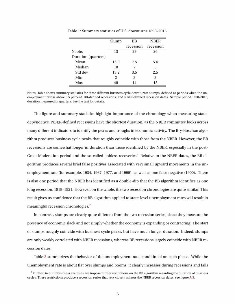
Table 1: Summary statistics of U.S. downturns 1890–2015.
Slump BB NBERrecession recession
N. obs 13 29 26Duration (quarters)
Mean 13.9 7.5 5.6Median 10 7 5Std dev 13.2 3.5 2.5Min 2 3 3Max 48 14 15
Notes: Table shows summary statistics for three different business cycle downturns: slumps, defined as periods when the un-employment rate is above 6.5 percent; BB-defined recessions; and NBER-defined recession dates. Sample period 1890–2015,duration measured in quarters. See the text for details.
The figure and summary statistics highlight importance of the chronology when measuring state-
dependence. NBER-defined recessions have the shortest duration, as the NBER committee looks across
many different indicators to identify the peaks and troughs in economic activity. The Bry-Boschan algo-
rithm produces business cycle peaks that roughly coincide with those from the NBER. However, the BB
recessions are somewhat longer in duration than those identified by the NBER, especially in the post-
Great Moderation period and the so-called ‘jobless recoveries.’ Relative to the NBER dates, the BB al-
gorithm produces several brief false positives associated with very small upward movements in the un-
employment rate (for example, 1934, 1967, 1977, and 1995), as well as one false negative (1900). There
is also one period that the NBER has identified as a double-dip that the BB algorithm identifies as one
long recession, 1918–1921. However, on the whole, the two recession chronologies are quite similar. This
result gives us confidence that the BB algorithm applied to state-level unemployment rates will result in
meaningful recession chronologies.7
In contrast, slumps are clearly quite different from the two recession series, since they measure the
presence of economic slack and not simply whether the economy is expanding or contracting. The start
of slumps roughly coincide with business cycle peaks, but have much longer duration. Indeed, slumps
are only weakly correlated with NBER recessions, whereas BB recessions largely coincide with NBER re-
cession dates.
Table 2 summarizes the behavior of the unemployment rate, conditional on each phase. While the
unemployment rate is about flat over slumps and booms, it clearly increases during recessions and falls
7Further, in our robustness exercises, we impose further restrictions on the BB algorithm regarding the duration of businesscycles. These restrictions produce a recession series that very closely mirrors the NBER recession dates, see figure A.3.
6
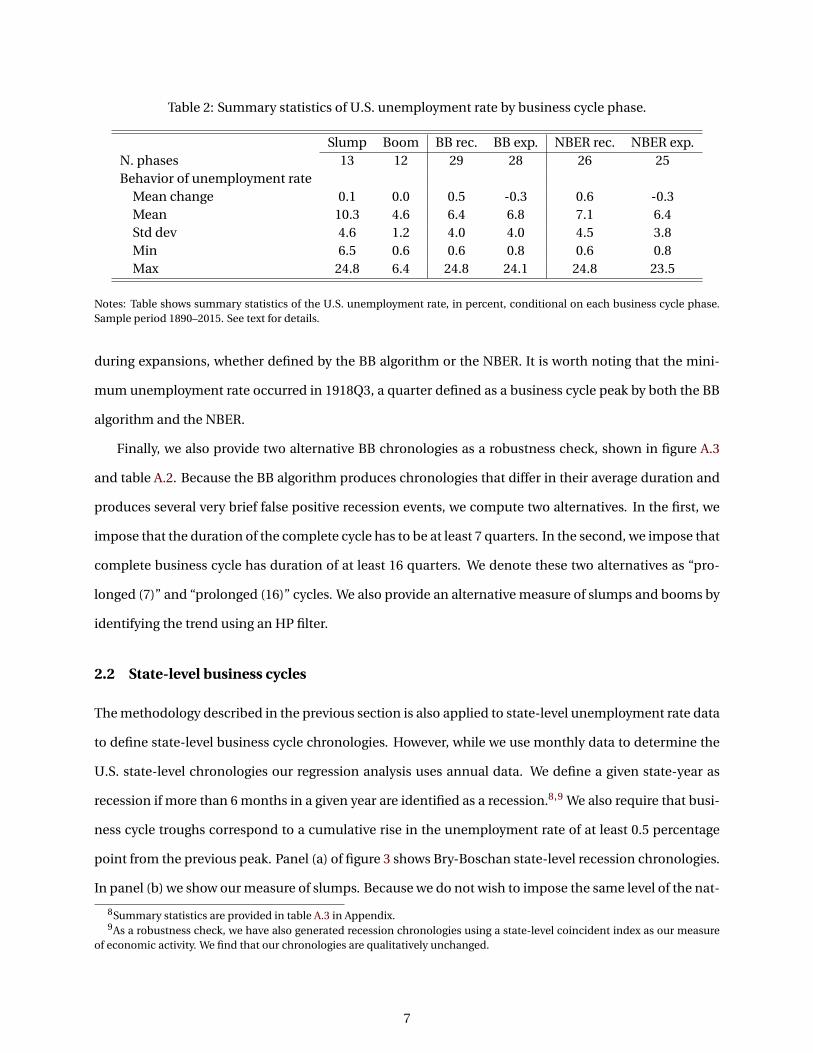
Table 2: Summary statistics of U.S. unemployment rate by business cycle phase.
Slump Boom BB rec. BB exp. NBER rec. NBER exp.N. phases 13 12 29 28 26 25Behavior of unemployment rate
Mean change 0.1 0.0 0.5 -0.3 0.6 -0.3Mean 10.3 4.6 6.4 6.8 7.1 6.4Std dev 4.6 1.2 4.0 4.0 4.5 3.8Min 6.5 0.6 0.6 0.8 0.6 0.8Max 24.8 6.4 24.8 24.1 24.8 23.5
Notes: Table shows summary statistics of the U.S. unemployment rate, in percent, conditional on each business cycle phase.Sample period 1890–2015. See text for details.
during expansions, whether defined by the BB algorithm or the NBER. It is worth noting that the mini-
mum unemployment rate occurred in 1918Q3, a quarter defined as a business cycle peak by both the BB
algorithm and the NBER.
Finally, we also provide two alternative BB chronologies as a robustness check, shown in figure A.3
and table A.2. Because the BB algorithm produces chronologies that differ in their average duration and
produces several very brief false positive recession events, we compute two alternatives. In the first, we
impose that the duration of the complete cycle has to be at least 7 quarters. In the second, we impose that
complete business cycle has duration of at least 16 quarters. We denote these two alternatives as “pro-
longed (7)” and “prolonged (16)” cycles. We also provide an alternative measure of slumps and booms by
identifying the trend using an HP filter.
2.2 State-level business cycles
The methodology described in the previous section is also applied to state-level unemployment rate data
to define state-level business cycle chronologies. However, while we use monthly data to determine the
U.S. state-level chronologies our regression analysis uses annual data. We define a given state-year as
recession if more than 6 months in a given year are identified as a recession.8,9 We also require that busi-
ness cycle troughs correspond to a cumulative rise in the unemployment rate of at least 0.5 percentage
point from the previous peak. Panel (a) of figure 3 shows Bry-Boschan state-level recession chronologies.
In panel (b) we show our measure of slumps. Because we do not wish to impose the same level of the nat-
8Summary statistics are provided in table A.3 in Appendix.9As a robustness check, we have also generated recession chronologies using a state-level coincident index as our measure
of economic activity. We find that our chronologies are qualitatively unchanged.
7
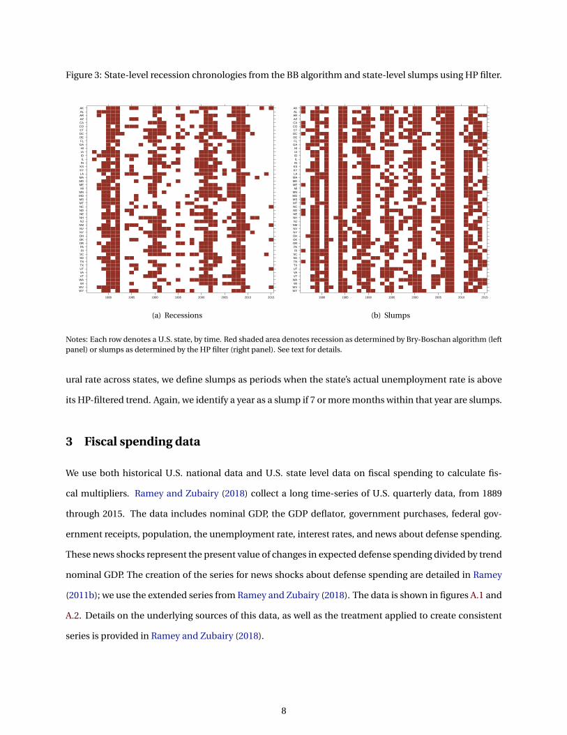
Figure 3: State-level recession chronologies from the BB algorithm and state-level slumps using HP filter.
WYWVWI
WAVTVAUTTXTNSDSCRIPA
OROKOHNYNVNMNJNHNENDNCMTMSMOMNMI
MEMDMALAKYKSINILIDIAHI
GAFLDEDCCTCOCAAZARALAK
1980 1985 1990 1995 2000 2005 2010 2015
(a) Recessions
WYWVWI
WAVTVAUTTXTNSDSCRIPA
OROKOHNYNVNMNJNHNENDNCMTMSMOMNMI
MEMDMALAKYKSINILIDIAHI
GAFLDEDCCTCOCAAZARALAK
1980 1985 1990 1995 2000 2005 2010 2015
(b) Slumps
Notes: Each row denotes a U.S. state, by time. Red shaded area denotes recession as determined by Bry-Boschan algorithm (leftpanel) or slumps as determined by the HP filter (right panel). See text for details.
ural rate across states, we define slumps as periods when the state’s actual unemployment rate is above
its HP-filtered trend. Again, we identify a year as a slump if 7 or more months within that year are slumps.
3 Fiscal spending data
We use both historical U.S. national data and U.S. state level data on fiscal spending to calculate fis-
cal multipliers. Ramey and Zubairy (2018) collect a long time-series of U.S. quarterly data, from 1889
through 2015. The data includes nominal GDP, the GDP deflator, government purchases, federal gov-
ernment receipts, population, the unemployment rate, interest rates, and news about defense spending.
These news shocks represent the present value of changes in expected defense spending divided by trend
nominal GDP. The creation of the series for news shocks about defense spending are detailed in Ramey
(2011b); we use the extended series from Ramey and Zubairy (2018). The data is shown in figures A.1 and
A.2. Details on the underlying sources of this data, as well as the treatment applied to create consistent
series is provided in Ramey and Zubairy (2018).
8
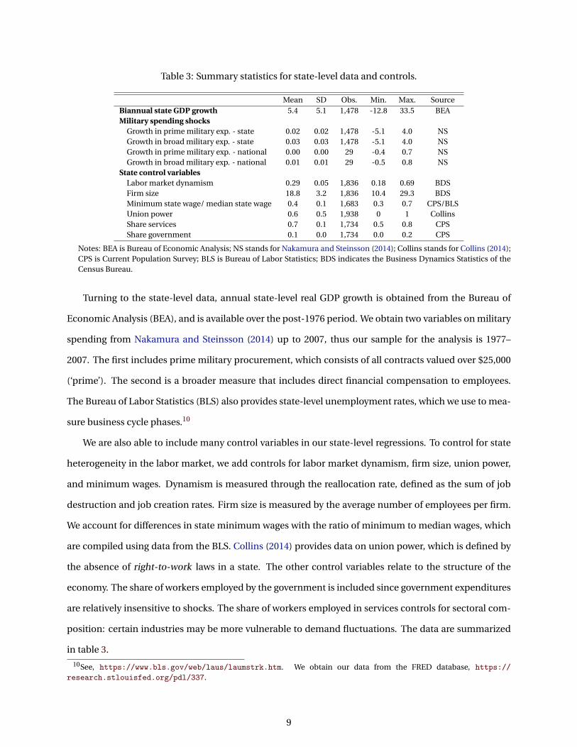
Table 3: Summary statistics for state-level data and controls.
Mean SD Obs. Min. Max. SourceBiannual state GDP growth 5.4 5.1 1,478 -12.8 33.5 BEAMilitary spending shocks
Growth in prime military exp. - state 0.02 0.02 1,478 -5.1 4.0 NSGrowth in broad military exp. - state 0.03 0.03 1,478 -5.1 4.0 NSGrowth in prime military exp. - national 0.00 0.00 29 -0.4 0.7 NSGrowth in broad military exp. - national 0.01 0.01 29 -0.5 0.8 NS
State control variablesLabor market dynamism 0.29 0.05 1,836 0.18 0.69 BDSFirm size 18.8 3.2 1,836 10.4 29.3 BDSMinimum state wage/ median state wage 0.4 0.1 1,683 0.3 0.7 CPS/BLSUnion power 0.6 0.5 1,938 0 1 CollinsShare services 0.7 0.1 1,734 0.5 0.8 CPSShare government 0.1 0.0 1,734 0.0 0.2 CPS
Notes: BEA is Bureau of Economic Analysis; NS stands for Nakamura and Steinsson (2014); Collins stands for Collins (2014);CPS is Current Population Survey; BLS is Bureau of Labor Statistics; BDS indicates the Business Dynamics Statistics of theCensus Bureau.
Turning to the state-level data, annual state-level real GDP growth is obtained from the Bureau of
Economic Analysis (BEA), and is available over the post-1976 period. We obtain two variables on military
spending from Nakamura and Steinsson (2014) up to 2007, thus our sample for the analysis is 1977–
2007. The first includes prime military procurement, which consists of all contracts valued over $25,000
(‘prime’). The second is a broader measure that includes direct financial compensation to employees.
The Bureau of Labor Statistics (BLS) also provides state-level unemployment rates, which we use to mea-
sure business cycle phases.10
We are also able to include many control variables in our state-level regressions. To control for state
heterogeneity in the labor market, we add controls for labor market dynamism, firm size, union power,
and minimum wages. Dynamism is measured through the reallocation rate, defined as the sum of job
destruction and job creation rates. Firm size is measured by the average number of employees per firm.
We account for differences in state minimum wages with the ratio of minimum to median wages, which
are compiled using data from the BLS. Collins (2014) provides data on union power, which is defined by
the absence of right-to-work laws in a state. The other control variables relate to the structure of the
economy. The share of workers employed by the government is included since government expenditures
are relatively insensitive to shocks. The share of workers employed in services controls for sectoral com-
position: certain industries may be more vulnerable to demand fluctuations. The data are summarized
in table 3.
10See, https://www.bls.gov/web/laus/laumstrk.htm. We obtain our data from the FRED database, https://
research.stlouisfed.org/pdl/337.
9

4 Revisiting state-dependence of the fiscal multiplier
We now estimate the fiscal multiplier across the phases of the business cycle identified in section 2. We
estimate the multiplier in two different ways. First we use the national military news shocks at the na-
tional level as introduced by Ramey (2011b) and recently updated in Ramey and Zubairy (2018). We then
turn to the panel data approach at the state level of Nakamura and Steinsson (2014).
4.1 Estimating fiscal multipliers with historical time-series
4.1.1 Empirical approach
The response of real government spending and real GDP to the news shocks identified in ? is measured
using the local projections of Jordà (2005):
yt+h =αy,h +βy,h shockt +γy,h zt−1 +εy,t+h (1)
g t+h =αg ,h +βg ,h shockt +γg ,h zt−1 +εg ,t+h . (2)
Here yt+h is the cumulative change in GDP between t and t+h, normalized by potential GDP in the initial
period as in Gordon and Krenn (2010):
yt+h = Yt+h/Y pt ,
where Y /Y p respectively denote actual and potential GDP. shockt is the identified fiscal spending shock
and z is a vector of controls. g t+h is the cumulative change in detrended government spending:
g t+h = (Gt+h −Gpt+h)/Y p
t ,
where Gp is the trend in government expenditures, measured as the residual from regressing government
spending on a fourth degree polynomial time trend. We detrend government spending as the ratio of
government spending to potential GDP has a secular upward trend. Failing to account for this trend in
the econometric specification will bias the ultimate estimate of the fiscal multiplier downwards, because
the local projections will confound exogenous increases in g with the trend.11 Figure 4 illustrates the
11In the state-level panel analysis we remove time trends through the inclusion of time fixed effects.
10

Figure 4: Real government expenditures before and after controlling for its secular trend.
1890 1900 1910 1920 1930 1940 1950 1960 1970 1980 1990 2000 2010
020
4060
%Real per capita government spending as a share of potential GDP
1890 1900 1910 1920 1930 1940 1950 1960 1970 1980 1990 2000 2010
020
40
%Detrended real per capita government spending as a share of potential GDP
Notes: Figure shows the raw and the detrended measure of real government expenditures per capita in the United States. Verticaldashed lines denote start of various wars (Spanish-American, WWI, WWII, Korean, Vietnam, response to Soviet invasion ofAfghanistan, and Sept 11, 2001). See text for details.
difference between the original and the detrended series.12 Methodologically, one could interpret this as
that we are calculating the multipliers of the discretionary part of government spending.
The βh coefficients in equations (1)–(2) give the average response of output or government expendi-
ture to a military news shock in horizon h. To estimate business cycle phase-dependent effect of defense
news on GDP, for example, the shocks and covariates are interacted with a dummy variable indicating the
phase of the business cycle:
yt+h = It−1(α1,h +β1,h shockt +γ1,h zt−1
)+ (1− It−1)
(α0,h +β0,h shockt +γ0,h zt−1
)+εt+h . (3)
The fiscal multiplier can then be calculated as the ratio of the cumulative effect of the news shock to
output relative to that on spending. Specifically, the cumulative multiplier m j over an H-quarter horizon
is:
m j =H∑
h=1βy, j ,h/
H∑h=1
βg , j ,h , (4)
where the subscript j denotes the fact that the multiplier may be either an average response or a phase-
dependent response.
12Alternatively, one could control for trends in the local projection analysis. We have found that the results are very similarbetween these alternatives, but that one should be careful when estimating state-dependent multipliers with trends, as thetwo procedures described above are no longer equivalent. It is also not clear whether state-dependent trends are conceptuallyappropriate. Thus, we have opted to adjust the transformation of variables to control for the secular trend in g .
11

An equivalent estimation of the multiplier can be obtained from an IV approach (Ramey and Zubairy,
2018). Specifically, we estimate IV regressions for each horizon h:
h∑j=0
yt+ j = It−1(α1,h +m1,h
h∑j=0
g t+ j +γ1,h zt−1)+ (
1− It−1)(α0,h +m0,h
h∑j=0
g t+ j +γ0,h zt−1)+ωt+h , (5)
using It−1 × shockt and (1− It−1)× shockt as instruments for accumulated government spending.
4.1.2 Results
We begin by examining instrument relevance. Our first-stage regression projects cumulated real govern-
ment spending at each horizon onto the news shock at period t. We consider two instrument sets: the
Ramey fiscal news shocks and the Ramey fiscal news shocks alongside the Blanchard and Perotti (2002)
shocks. The Blanchard-Perotti shocks are identified within a Vector Autoregression with government
spending, GDP, and taxes using a Cholesky decomposition where government spending is ordered first.
Thus, it relies on the assumption that within-quarter government spending does not respond to these
macroeconomic variables contemporaneously.13
We also condition on four lags each of GDP, government expenditure, and controls.14 Figure 5 plots
the difference between the first-stage effective F-statistics and the thresholds computed in Montiel Olea
and Pflueger (2013). The purple lines are the values of the F-statistic relative to the threshold when using
only the military news shocks as the instrument, while the asterisked orange line shows the value with
both instruments. The figure suggests that military news has high relevance during slumps, but otherwise
the F-statistic remains below the relevant thresholds for other cases considered, including the linear case.
In general, using both shocks appears to be a more powerful instrument than the military news shock
alone, although at longer horizons the F-statistics tend to fall below the relevant thresholds.
Table 4 presents multiple estimates of the cumulative fiscal multiplier. Column 2 contains multipliers
from the linear model. Columns 3-4 contain results for slumps and booms, while the rightmost columns
present the results calculated over recessions and expansions. For each regression specification we cu-
mulate the fiscal multiplier over a two year and four year period. The blocks of the table present different
regression specifications. The baseline specification uses the same controls as Ramey and Zubairy (2018),
13Ramey and Zubairy point out that the Blanchard-Perotti shocks are sensitive to potential measurement error in governmentspending and potentially anticipated, which is why they are only included as robustness checks.
14The vector of control variables includes the ratio of GDP to potential, the ratio of government spending to potential, lags ofthose two controls, and lagged news shocks.
12
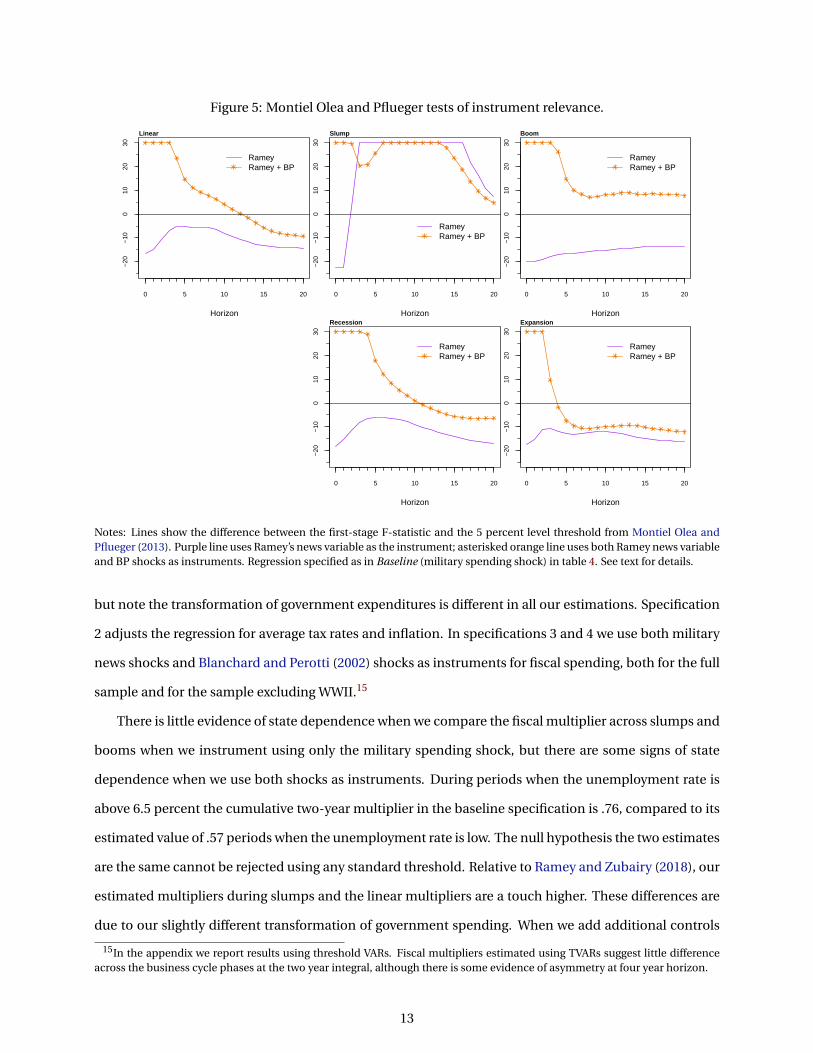
Figure 5: Montiel Olea and Pflueger tests of instrument relevance.
Horizon
0 5 10 15 20
−20
−10
010
2030
Linear
RameyRamey + BP
Horizon
0 5 10 15 20
−20
−10
010
2030
Slump
RameyRamey + BP
Horizon
0 5 10 15 20
−20
−10
010
2030
Boom
RameyRamey + BP
Horizon
0 5 10 15 20
−20
−10
010
2030
Recession
RameyRamey + BP
Horizon
0 5 10 15 20
−20
−10
010
2030
Expansion
RameyRamey + BP
Notes: Lines show the difference between the first-stage F-statistic and the 5 percent level threshold from Montiel Olea andPflueger (2013). Purple line uses Ramey’s news variable as the instrument; asterisked orange line uses both Ramey news variableand BP shocks as instruments. Regression specified as in Baseline (military spending shock) in table 4. See text for details.
but note the transformation of government expenditures is different in all our estimations. Specification
2 adjusts the regression for average tax rates and inflation. In specifications 3 and 4 we use both military
news shocks and Blanchard and Perotti (2002) shocks as instruments for fiscal spending, both for the full
sample and for the sample excluding WWII.15
There is little evidence of state dependence when we compare the fiscal multiplier across slumps and
booms when we instrument using only the military spending shock, but there are some signs of state
dependence when we use both shocks as instruments. During periods when the unemployment rate is
above 6.5 percent the cumulative two-year multiplier in the baseline specification is .76, compared to its
estimated value of .57 periods when the unemployment rate is low. The null hypothesis the two estimates
are the same cannot be rejected using any standard threshold. Relative to Ramey and Zubairy (2018), our
estimated multipliers during slumps and the linear multipliers are a touch higher. These differences are
due to our slightly different transformation of government spending. When we add additional controls
15In the appendix we report results using threshold VARs. Fiscal multipliers estimated using TVARs suggest little differenceacross the business cycle phases at the two year integral, although there is some evidence of asymmetry at four year horizon.
13

Table 4: Estimated fiscal multipliers.
Linear Above/below trend Peak to trough (BB alg)All Slump Boom Recession Expansion
1. Baseline (military spending shock)2 year integral 0.72 0.76 0.57 1.60 0.64†
(0.09) (0.11) (0.10) (0.42) (0.11)4 year integral 0.78 0.76 0.63 1.93 0.74†
(0.06) (0.05) (0.10) (0.57) (0.08)2. Military spending shock, taxes and inflation as additional controls
2 year integral 0.74 0.86 0.63 1.28 0.67(0.09) (0.17) (0.10) (0.33) (0.09)
4 year integral 0.79 0.82 0.66 1.48 0.78(0.07) (0.08) (0.12) (0.46) (0.06)
3. Military spending shock + BP shocks2 year integral 0.50 0.83 0.42† 0.88 0.54
(0.08) (0.18) (0.08) (0.28) (0.11)4 year integral 0.71 0.75 0.56† 1.37 0.69†
(0.06) (0.05) (0.08) (0.41) (0.09)4. Military spending shock + BP shocks, excluding WWII
2 year integral 0.47 1.94 0.33† 0.57 0.42(0.16) (0.83) (0.13) (0.37) (0.26)
4 year integral 0.77 1.67 0.59 1.20 0.59(0.35) (0.71) (0.31) (0.48) (0.52)
Notes: Newey-West standard errors in parentheses. BP denotes Blanchard and Perotti (2002). Specification 4 excludes ob-servations from 1941Q3 to 1945Q4. See text for details.† indicates that the difference across phases is statistically significant at 10 percent level.
for taxes and inflation, the estimated multiplier increases, especially during slumps, but remains sta-
tistically indistinguishable from the boom-time multiplier. Finally, the estimates of the fiscal multiplier
are below one; the only specification where slump-specific multiplier is larger than one occurs when we
exclude WWII.
Results that compare recessions and expansions are somewhat different. In the baseline specifica-
tion, the two-year cumulative multiplier is 1.6 in recessions, compared to .6 during expansions, a statis-
tically relevant difference at the 5 percent level. The standard errors of the recession multipliers are sig-
nificantly larger than those from the slump/boom chronologies, reflecting a relative lack of data points
during recessions. The difference between the estimated multiplier in a recession versus an expansion is
typically not statistically different in the other specifications, although the estimated multiplier is always
higher in recessions than expansions.
Figure 6 presents cumulated multipliers for the baseline specification. The left panel compares booms
and slumps, while the right panel shows recessions versus expansions. This figure shows a clear state-
dependence in the multiplier when comparing recessions to expansions, whereas the multiplier is very
14
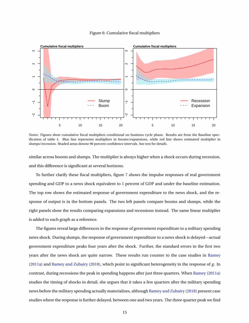
Figure 6: Cumulative fiscal multipliers
5 10 15 20
−2
−1
01
23
Cumulative fiscal multipliers
SlumpBoom
5 10 15 20−
2−
10
12
3
Cumulative fiscal multipliers
RecessionExpansion
Notes: Figures show cumulative fiscal multipliers conditional on business cycle phase. Results are from the Baseline spec-ification of table 4. Blue line represents multipliers in booms/expansions, while red line shows estimated multiplier inslumps/recession. Shaded areas denote 90 percent confidence intervals. See text for details.
similar across booms and slumps. The multiplier is always higher when a shock occurs during recession,
and this difference is significant at several horizons.
To further clarify these fiscal multipliers, figure 7 shows the impulse responses of real government
spending and GDP to a news shock equivalent to 1 percent of GDP and under the baseline estimation.
The top row shows the estimated response of government expenditure to the news shock, and the re-
sponse of output is in the bottom panels. The two left panels compare booms and slumps, while the
right panels show the results comparing expansions and recessions instead. The same linear multiplier
is added to each graph as a reference.
The figures reveal large differences in the response of government expenditure to a military spending
news shock. During slumps, the response of government expenditure to a news shock is delayed—actual
government expenditure peaks four years after the shock. Further, the standard errors in the first two
years after the news shock are quite narrow. These results run counter to the case studies in Ramey
(2011a) and Ramey and Zubairy (2018), which point to significant heterogeneity in the response of g . In
contrast, during recessions the peak in spending happens after just three quarters. When Ramey (2011a)
studies the timing of shocks in detail, she argues that it takes a few quarters after the military spending
news before the military spending actually materializes, although Ramey and Zubairy (2018) present case
studies where the response is further delayed, between one and two years. The three quarter peak we find
15

Figure 7: Phase-specific response of government spending and GDP to a news shock.
5 10 15 20
0.0
0.2
0.4
0.6
0.8
1.0
Quarters
Govt spending response in slump/boom %
SlumpBoomLinear
5 10 15 20
0.0
0.5
1.0
1.5
Quarters
Govt spending response in recession/expansion %
RecessionExpansionLinear
5 10 15 20
0.0
0.2
0.4
0.6
0.8
1.0
Quarters
GDP response in slump/boom %
SlumpBoomLinear
5 10 15 20
0.0
0.5
1.0
1.5
Quarters
%GDP response in recession/expansion
RecessionExpansionLinear
Notes: Panels show phase-specific response of government expenditure (top row) and GDP (bottom row) to a military expendi-ture news shock scaled to 1 percent of GDP. Regression specification is the baseline specification in table 4. Red lines show theresponse in slumps (left) or recessions (right). Blue line is the response in booms (left) or expansions (right). Black lines are theresponse from the linear model. Shaded areas denote 90 percent confidence intervals.
during recessions is consistent with the event study for both the the Korean and the Vietnam wars. Dur-
ing the First and Second World Wars, government spending increased immediately following the news
shocks, and peaked six to eight quarters after. In addition, during recessions government spending re-
mains at the elevated level for several years. This is in line with the case studies of several wars mentioned
above. All told, while there is substantial heterogeneity in the response of government spending after the
news, we believe that the response during recessions is more consistent with the event studies mentioned
above than the response shown for slumps.
16

Putting the responses of government expenditure and output together, one can reconcile the multi-
pliers from figure 6 by mentally applying equation 4. In recessions, the response of government expen-
diture is front-loaded and peaks at a smaller level than the response during slumps. At the same time,
the response of output is cumulatively larger in recessions than in expansions, especially in the first two
years after the shock. (Because there are few news shocks during our identified recessions, the responses
of both government expenditure and output are very uncertain.) In contrast, as we can see by the re-
sponse of government expenditure during slumps, the bulk of government expenditure is quite delayed
from the news shock itself. Given that the average recession in our sample lasts just over 1.5 years, it is
unlikely that government expenditure actually occurs during periods of severe economic distress. The
response of output itself is also ultimately smaller. Overall, we view these results as supporting the idea
that fiscal multipliers are larger during periods of economic distress, but emphasize that the period of
time in which the multiplier is relatively large may be quite short.
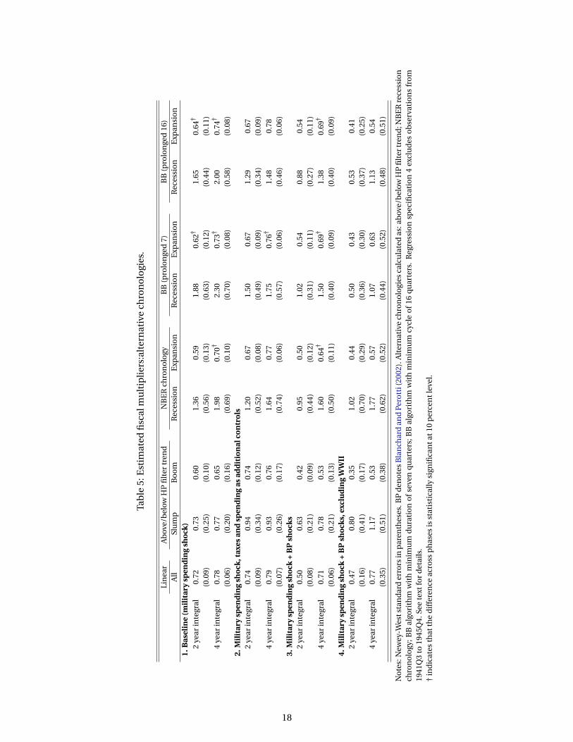
4.1.3 Robustness checks
In this subsection we document the robustness of our results to several different business cycle chronolo-
gies, shown in figure A.3. The multipliers associated with these alternative chronologies are given in table
5. The first alternative chronology we calculate is an alternative slumps/boom chronology, where we de-
fine slumps as periods when the unemployment rate is below or above its HP-filter implied trend. The
results are qualitatively similar to those for slumps and booms based on a fixed threshold of 6.5 percent.
For the chronology based on the HP filter trend, the multiplier is always estimated to be higher in slumps
than in booms, but as before, the difference is not statistically meaningful.
Next, we recompute fiscal multipliers under three different definitions of recession. The resulting
estimates of the fiscal multiplier are in the remaining columns of table 5. Our results are on the whole
robust to the alternative recession/expansion chronologies. For each chronology and regression speci-
fication, we find that the multiplier is higher in recession than in expansion, although the difference is
not always statistically relevant. The estimated multiplier in expansions is typically around 0.5, while in
recession, the estimated multiplier often exceeds one. Since the NBER business cycle chronology is quite
similar to the chronology based on the Bry-Boschan algorithm, it is not surprising that the results using
the NBER’s chronology are by and large similar to those presented in the previous section. The results of
the two prolonged BB chronologies are also quite similar to the original results.
17
Tab
le5:
Est
imat
edfi
scal
mu
ltip
lier
s:al
tern
ativ
ech
ron
olo
gies
.
Lin
ear
Ab
ove/
bel
owH
Pfi
lter
tren
dN
BE
Rch
ron
olo
gyB
B(p
rolo
nge
d7)
BB
(pro
lon
ged
16)
All
Slu
mp
Bo
om
Rec
essi
on
Exp
ansi
on
Rec
essi
on
Exp
ansi
on
Rec
essi
on
Exp
ansi
on
1.B
asel
ine
(mil
itar
ysp
end
ing
sho
ck)
2ye
arin
tegr
al0.
720.
730.
601.
360.
591.
880.
62†
1.65
0.64
†
(0.0
9)(0
.25)
(0.1
0)(0
.56)
(0.1
3)(0
.63)
(0.1
2)(0
.44)
(0.1
1)4
year
inte
gral
0.78
0.77
0.65
1.98
0.70
†2.
300.
73†
2.00
0.74
†
(0.0
6)(0
.20)
(0.1
6)(0
.69)
(0.1
0)(0
.70)
(0.0
8)(0
.58)
(0.0
8)2.
Mil
itar
ysp
end
ing
sho
ck,t
axes
and
spen
din
gas
add
itio
nal
con
tro
ls2
year
inte
gral
0.74
0.94
0.74
1.20
0.67
1.50
0.67
1.29
0.67
(0.0
9)(0
.34)
(0.1
2)(0
.52)
(0.0
8)(0
.49)
(0.0
9)(0
.34)
(0.0
9)4
year
inte
gral
0.79
0.93
0.76
1.64
0.77
1.75
0.76
†1.
480.
78(0
.07)
(0.2
6)(0
.17)
(0.7
4)(0
.06)
(0.5
7)(0
.06)
(0.4
6)(0
.06)
3.M
ilit
ary
spen
din
gsh
ock
+B
Psh
ock
s2
year
inte
gral
0.50
0.63
0.42
0.95
0.50
1.02
0.54
0.88
0.54
(0.0
8)(0
.21)
(0.0
9)(0
.44)
(0.1
2)(0
.31)
(0.1
1)(0
.27)
(0.1
1)4
year
inte
gral
0.71
0.78
0.53
1.60
0.64
†1.
500.
69†
1.38
0.69
†
(0.0
6)(0
.21)
(0.1
3)(0
.50)
(0.1
1)(0
.40)
(0.0
9)(0
.40)
(0.0
9)4.
Mil
itar
ysp
end
ing
sho
ck+
BP
sho
cks,
excl
ud
ing
WW
II2
year
inte
gral
0.47
0.80
0.35
1.02
0.44
0.50
0.43
0.53
0.41
(0.1
6)(0
.41)
(0.1
7)(0
.70)
(0.2
9)(0
.36)
(0.3
0)(0
.37)
(0.2
5)4
year
inte
gral
0.77
1.17
0.53
1.77
0.57
1.07
0.63
1.13
0.54
(0.3
5)(0
.51)
(0.3
8)(0
.62)
(0.5
2)(0
.44)
(0.5
2)(0
.48)
(0.5
1)
No
tes:
New
ey-W
ests
tan
dar
der
rors
inp
aren
thes
es.B
Pd
eno
tes
Bla
nch
ard
and
Pero
tti(
2002
).A
lter
nat
ive
chro
no
logi
esca
lcu
late
das
:ab
ove/
bel
owH
Pfi
lter
tren
d;N
BE
Rre
cess
ion
chro
no
logy
;BB
algo
rith
mw
ith
min
imu
md
ura
tio
no
fse
ven
qu
arte
rs;B
Bal
gori
thm
wit
hm
inim
um
cycl
eo
f16
qu
arte
rs.
Reg
ress
ion
spec
ifica
tio
n4
excl
ud
eso
bse
rvat
ion
sfr
om
1941
Q3
to19
45Q
4.Se
ete
xtfo
rd
etai
ls.
†in
dic
ates
that
the
dif
fere
nce
acro
ssp
has
esis
stat
isti
cally
sign
ifica
nta
t10
per
cen
tlev
el.
18

4.2 State-level analysis using military spending shocks
We next show that we again find evidence that the fiscal multiplier varies across the business cycle when
we follow the approach of Nakamura and Steinsson (2014). Nakamura and Steinsson identify exoge-
nous variation in state-level fiscal policy by assuming that the federal government does not alter national
spending in response to the relative performance of the U.S. states.16 This approach has the advantage
that it introduces a panel element to the data, which may improve the precision of the estimates of the fis-
cal multiplier. By allowing for the inclusion of time-fixed effects, the panel structure furthermore allows
us to control for potentially state-dependent responses of monetary policy. Since we produce business
cycle chronologies at the state level, we add tests of whether the multiplier differs across the four business
cycle phases.
Nakamura and Steinsson (2014) estimate a two-stage instrumental variables regression. In the first
stage, the change in military spending at the state level is regressed onto the change in national military
spending and controls:
∆µs,t =βs∆µnat ,t + Is,t−1(α1,s +ξ1,s(L)zt
)+ (1− Is,t−1
)(α0,s +ξ0,s(L)zt
)+Φ′scs,t +εs,t , (6)
where µs and µnat are biannual changes in state and federal military expenditure as a percentage of GDP,
z is a vector of controls, and c are fixed effects. Ist is the dummy variable that indicates the state of the
business cycle in state s at period t . The second stage regression regresses the fitted values from the first
stage onto state-level GDP:
∆ys,t = Is,t−1(α0,s +ψ0,s(L)zt +γ0∆µs,t
)+ (1− Is,t−1
)(α1,s +ψ1,s(L)zt +γ1∆µs,t
)+φ′scs,t +ηs,t , (7)
where ∆y measures biannual growth in state GDP while µ denotes the fitted value of equation 6. The
parameters γ0 and γ1 capture the phase-dependent multipliers. It is worth emphasizing that these equa-
tions estimate an open economy relative multiplier for federal spending, which quantifies increases in
16Compared to the analysis in Nakamura and Steinsson (2014), we use a shorter sample, without the Korean war, as advocatedby Dupor and Guerrero (2017).
19
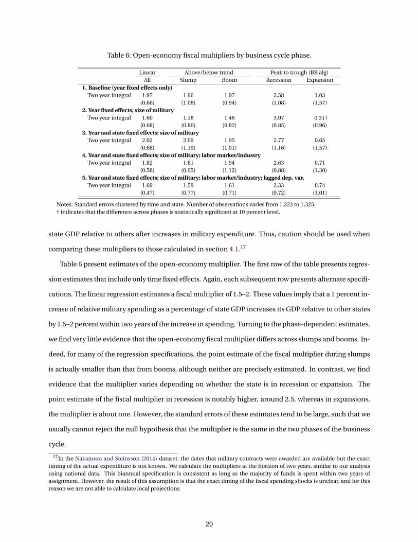
Table 6: Open-economy fiscal multipliers by business cycle phase.
Linear Above/below trend Peak to trough (BB alg)All Slump Boom Recession Expansion
1. Baseline (year fixed effects only)Two year integral 1.97 1.96 1.97 2.58 1.03
(0.66) (1.08) (0.94) (1.08) (1.57)2. Year fixed effects; size of military
Two year integral 1.60 1.18 1.46 3.07 -0.31†(0.68) (0.86) (0.82) (0.85) (0.96)
3. Year and state fixed effects; size of militaryTwo year integral 2.02 2.09 1.95 2.77 0.65
(0.68) (1.19) (1.01) (1.16) (1.57)4. Year and state fixed effects; size of military; labor market/industry
Two year integral 1.82 1.81 1.94 2.63 0.71(0.58) (0.95) (1.12) (0.88) (1.30)
5. Year and state fixed effects; size of military; labor market/industry; lagged dep. var.Two year integral 1.69 1.59 1.61 2.33 0.74
(0.47) (0.77) (0.71) (0.72) (1.01)
Notes: Standard errors clustered by time and state. Number of observations varies from 1,223 to 1,325.† indicates that the difference across phases is statistically significant at 10 percent level.
state GDP relative to others after increases in military expenditure. Thus, caution should be used when
comparing these multipliers to those calculated in section 4.1.17
Table 6 present estimates of the open-economy multiplier. The first row of the table presents regres-
sion estimates that include only time fixed effects. Again, each subsequent row presents alternate specifi-
cations. The linear regression estimates a fiscal multiplier of 1.5–2. These values imply that a 1 percent in-
crease of relative military spending as a percentage of state GDP increases its GDP relative to other states
by 1.5–2 percent within two years of the increase in spending. Turning to the phase-dependent estimates,
we find very little evidence that the open-economy fiscal multiplier differs across slumps and booms. In-
deed, for many of the regression specifications, the point estimate of the fiscal multiplier during slumps
is actually smaller than that from booms, although neither are precisely estimated. In contrast, we find
evidence that the multiplier varies depending on whether the state is in recession or expansion. The
point estimate of the fiscal multiplier in recession is notably higher, around 2.5, whereas in expansions,
the multiplier is about one. However, the standard errors of these estimates tend to be large, such that we
usually cannot reject the null hypothesis that the multiplier is the same in the two phases of the business
cycle.
17In the Nakamura and Steinsson (2014) dataset, the dates that military contracts were awarded are available but the exacttiming of the actual expenditure is not known. We calculate the multipliers at the horizon of two years, similar to our analysisusing national data. This biannual specification is consistent as long as the majority of funds is spent within two years ofassignment. However, the result of this assumption is that the exact timing of the fiscal spending shocks is unclear, and for thisreason we are not able to calculate local projections.
20
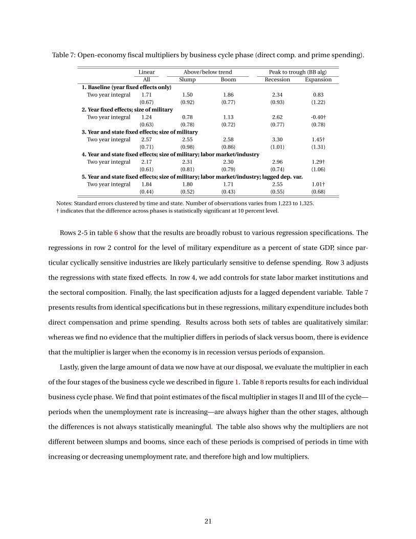
Table 7: Open-economy fiscal multipliers by business cycle phase (direct comp. and prime spending).
Linear Above/below trend Peak to trough (BB alg)All Slump Boom Recession Expansion
1. Baseline (year fixed effects only)Two year integral 1.71 1.50 1.86 2.34 0.83
(0.67) (0.92) (0.77) (0.93) (1.22)2. Year fixed effects; size of military
Two year integral 1.24 0.78 1.13 2.62 -0.40†(0.63) (0.78) (0.72) (0.77) (0.78)
3. Year and state fixed effects; size of militaryTwo year integral 2.57 2.55 2.58 3.30 1.45†
(0.71) (0.98) (0.86) (1.01) (1.31)4. Year and state fixed effects; size of military; labor market/industry
Two year integral 2.17 2.31 2.30 2.96 1.29†(0.61) (0.81) (0.79) (0.74) (1.06)
5. Year and state fixed effects; size of military; labor market/industry; lagged dep. var.Two year integral 1.84 1.80 1.71 2.55 1.01†
(0.44) (0.52) (0.43) (0.55) (0.68)
Notes: Standard errors clustered by time and state. Number of observations varies from 1,223 to 1,325.† indicates that the difference across phases is statistically significant at 10 percent level.
Rows 2-5 in table 6 show that the results are broadly robust to various regression specifications. The
regressions in row 2 control for the level of military expenditure as a percent of state GDP, since par-
ticular cyclically sensitive industries are likely particularly sensitive to defense spending. Row 3 adjusts
the regressions with state fixed effects. In row 4, we add controls for state labor market institutions and
the sectoral composition. Finally, the last specification adjusts for a lagged dependent variable. Table 7
presents results from identical specifications but in these regressions, military expenditure includes both
direct compensation and prime spending. Results across both sets of tables are qualitatively similar:
whereas we find no evidence that the multiplier differs in periods of slack versus boom, there is evidence
that the multiplier is larger when the economy is in recession versus periods of expansion.
Lastly, given the large amount of data we now have at our disposal, we evaluate the multiplier in each
of the four stages of the business cycle we described in figure 1. Table 8 reports results for each individual
business cycle phase. We find that point estimates of the fiscal multiplier in stages II and III of the cycle—
periods when the unemployment rate is increasing—are always higher than the other stages, although
the differences is not always statistically meaningful. The table also shows why the multipliers are not
different between slumps and booms, since each of these periods is comprised of periods in time with
increasing or decreasing unemployment rate, and therefore high and low multipliers.
21

Table 8: Estimated open economy fiscal multipliers by phase of business cycle.
Linear Stage I Stage IIAll Stage I Other stages Stage II Other stages
1. Baseline (year fixed effects only)Two year integral 1.97 0.88 2.37 2.93 1.58
(0.66) (1.41) (0.99) (1.24) (1.08)2. Year fixed effects; size of military
Two year integral 1.60 0.15 1.76 3.31 0.75†(0.68) (0.88) (0.87) (1.12) (0.74)
3. Year and state fixed effects; size of militaryTwo year integral 2.02 0.55 2.42 3.05 1.54
(0.68) (1.24) (1.10) (1.38) (1.16)4. Year and state fixed effects; size of military; labor market/industry
Two year integral 1.82 1.28 1.90 3.18 1.64(0.58) (1.23) (0.99) (1.20) (0.95)
5. Year and state fixed effects; size of military; labor market/industry; lagged dep. var.Two year integral 1.69 1.37 1.65 2.29 1.51
(0.47) (0.89) (0.75) (0.98) (0.71)
Linear Stage III Stage IVAll Stage III Other stages Stage IV Other stages
1. Baseline (year fixed effects only)Two year integral 1.97 2.22 1.85 1.46 2.04
(0.66) (1.28) (1.08) (2.12) (0.93)2. Year fixed effects; size of military
Two year integral 1.60 3.15 0.67† -0.36 1.84†(0.68) (0.82) (0.86) (1.28) (0.75)
3. Year and state fixed effects; size of militaryTwo year integral 2.02 2.48 1.79 1.34 2.13
(0.68) (1.38) (1.13) (1.94) (1.04)4. Year and state fixed effects; size of military; labor market/industry
Two year integral 1.82 2.43 1.33 1.23 1.97(0.58) (0.91) (1.24) (1.57) (0.95)
5. Year and state fixed effects; size of military; labor market/industry; lagged dep. var.Two year integral 1.69 2.26 1.22 0.65 1.81
(0.47) (0.73) (0.85) (1.42) (0.71)
Notes: Table reports estimates from the two-stage GMM estimator in equations 6 and 7. Phases correspond to those labeledin figure 1. Numbers in parentheses are standard errors, clustered by time and state. Number of observations varies from1,223 to 1,325.† indicates that the difference across phases is statistically significant at 10 percent level.
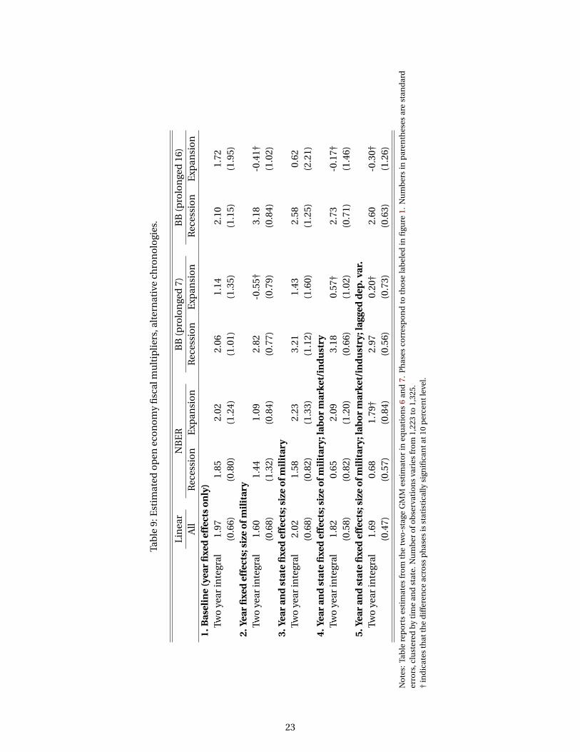
4.2.1 Robustness checks
We perform several robustness checks of our estimated open-economy fiscal multipliers. As before, we
check for the robustness using a different definition of recessions and/expansions.18 Results using these
alternative chronologies—the NBER dates and the two prolonged Bry-Boschan chronologies—are re-
ported in table 9.
18Because we do not believe the 6.5 percent threshold is sensible for all states, our baseline slump/boom chronology is basedon each state’s HP filtered unemployment rate. We do not present results for an alternative slump/boom chronology.
22
Tab
le9:
Est
imat
edo
pen
eco
no
my
fisc
alm
ult
ipli
ers,
alte
rnat
ive
chro
no
logi
es.
Lin
ear
NB
ER
BB
(pro
lon
ged
7)B
B(p
rolo
nge
d16
)A
llR
eces
sio
nE
xpan
sio
nR
eces
sio
nE
xpan
sio
nR
eces
sio
nE
xpan
sio
n1.
Bas
elin
e(y
ear
fixe
def
fect
so
nly
)Tw
oye
arin
tegr
al1.
971.
852.
022.
061.
142.
101.
72(0
.66)
(0.8
0)(1
.24)
(1.0
1)(1
.35)
(1.1
5)(1
.95)
2.Ye
arfi
xed
effe
cts;
size
ofm
ilit
ary
Two
year
inte
gral
1.60
1.44
1.09
2.82
-0.5
5†3.
18-0
.41†
(0.6
8)(1
.32)
(0.8
4)(0
.77)
(0.7
9)(0
.84)
(1.0
2)3.
Year
and
stat
efi
xed
effe
cts;
size
ofm
ilit
ary
Two
year
inte
gral
2.02
1.58
2.23
3.21
1.43
2.58
0.62
(0.6
8)(0
.82)
(1.3
3)(1
.12)
(1.6
0)(1
.25)
(2.2
1)4.
Year
and
stat
efi
xed
effe
cts;
size
ofm
ilit
ary;
lab
or
mar
ket/
ind
ust
ryTw
oye
arin
tegr
al1.
820.
652.
093.
180.
57†
2.73
-0.1
7†(0
.58)
(0.8
2)(1
.20)
(0.6
6)(1
.02)
(0.7
1)(1
.46)
5.Ye
aran
dst
ate
fixe
def
fect
s;si
zeo
fmil
itar
y;la
bo
rm
arke
t/in
du
stry
;lag
ged
dep
.var
.Tw
oye
arin
tegr
al1.
690.
681.
79†
2.97
0.20
†2.
60-0
.30†
(0.4
7)(0
.57)
(0.8
4)(0
.56)
(0.7
3)(0
.63)
(1.2
6)
No
tes:
Tab
lere
po
rts
esti
mat
esfr
om
the
two
-sta
geG
MM
esti
mat
or
ineq
uat
ion
s6
and
7.P
has
esco
rres
po
nd
toth
ose
lab
eled
infi
gure
1.N
um
ber
sin
par
enth
eses
are
stan
dar
der
rors
,clu
ster
edb
yti
me
and
stat
e.N
um
ber
ofo
bse
rvat
ion
sva
ries
fro
m1,
223
to1,
325.
†in
dic
ates
that
the
dif
fere
nce
acro
ssp
has
esis
stat
isti
cally
sign
ifica
nta
t10
per
cen
tlev
el.
23

The evidence for phase-dependence of the fiscal multiplier using these alternate specifications is
more mixed. For the NBER chronology, we find that the multiplier is actually smaller in recessions for
certain regression specifications. In contrast, alternative BB algorithms again show evidence that multi-
pliers differ across recessions and expansions. Indeed, the difference between recessions and expansions
is often more pronounced under these alternative chronologies and more often statistically significant at
standard levels.
5 Conclusion
This paper revisits the question of whether fiscal multipliers are larger in recessions than in expansions.
By separating the business cycle into four phases, we are able to reconcile conflicting results in previous
work. We view the bulk of the evidence presented here as supporting the idea that the fiscal spending
multiplier is larger in recessions than expansions. In contrast, there is scant evidence that the multiplier
varies when the unemployment rate is above or below its trend. We interpret these results as a synthesis
of the often conflicting results found in the literature.
Our results imply that policies that aim to reduce the volatility of economic activity and unemploy-
ment are most effective in recessions characterized by increasing unemployment. Even when unemploy-
ment is low and the output gap is positive, fiscal policy has the ability to cause a disproportionate increase
in output. When unemployment is falling, however, fiscal policy is less effective. Multipliers are below 1,
even when the level of unemployment remains high. Policymakers should therefore base decisions about
expansionary policies on the direction of change rather than on the level of the unemployment rate.
24

References
Auerbach, A. J. and Gorodnichenko, Y. (2012a). Fiscal Multipliers in Recession and Expansion. In Fiscal
Policy after the Financial Crisis, NBER Chapters, pages 63–98. National Bureau of Economic Research,
Inc.
Auerbach, A. J. and Gorodnichenko, Y. (2012b). Measuring the output responses to fiscal policy. American
Economic Journal: Economic Policy, 4(2):1–27.
Bachmann, R. and Sims, E. R. (2012). Confidence and the transmission of government spending shocks.
Journal of Monetary Economics, 59(3):235 – 249.
Baum, A., Poplawski-Ribeiro, M., and Weber, A. (2012). Fiscal Multipliers and the State of the Economy.
IMF Working Papers 12/286, International Monetary Fund.
Berge, T. J. and Pfajfar, D. (2019). Duration Dependence, Monetary Policy Asymmetries, and the Business
Cycle.
Blanchard, O. and Perotti, R. (2002). An empirical characterization of the dynamic effects of changes in
government spending and taxes on output. The Quarterly Journal of Economics, 117(4):1329–1368.
Blanchard, O. J. and Katz, L. F. (1992). Regional Evolutions. Brookings Papers on Economic Activity,
23(1):1–76.
Blanchard, O. j. and Leigh, D. (2013). Growth forecast errors and fiscal multipliers. American Economic
Review, 103(3):117–20.
Bry, G. and Boschan, C. (1972). Cyclical analysis of time series: selected procedures and computer pro-
grams. NBER.
Bureau of Labor Statistics (2017). Technical notes to establishment data published in employment and
earnings. Technical report, Bureau of Labor Statistics.
Candelon, B. and Lieb, L. (2013). Fiscal policy in good and bad times. Journal of Economic Dynamics and
Control, 37(12):2679 – 2694.
Canzoneri, M., Collard, F., Dellas, H., and Diba, B. (2016). Fiscal multipliers in recessions. The Economic
Journal, 126(590):75–108.
25

Carlino, G. and Defina, R. (1998). The Differential Regional Effects Of Monetary Policy. The Review of
Economics and Statistics, 80(4):572–587.
Christiano, L., Eichenbaum, M., and Rebelo, S. (2011). When is the government spending multiplier large?
Journal of Political Economy, 119(1):78–121.
Collins, B. (2014). Right to work laws: Legislative background and empirical research. Congressional
research service report, Congressional Research Service.
Driscoll, J. C. (2004). Does bank lending affect output? Evidence from the U.S. states. Journal of Monetary
Economics, 51(3):451–471.
Dupor, B. and Guerrero, R. (2017). Local and aggregate fiscal policy multipliers. Journal of Monetary
Economics, 92:16 – 30.
Fazzari, S., Morley, J., and Irina, P. (2015). State-dependent effects of fiscal policy. Studies in Nonlinear
Dynamics & Econometrics, 19(3):285–315.
Francis, N., Jackson, L. E., and Owyang, M. T. (2018). Countercyclical policy and the speed of recovery
after recessions. Journal of Money, Credit & Banking.
Gordon, R. J. and Krenn, R. (2010). The end of the great depression 1939-41: Policy contributions and
fiscal multipliers. Working Paper 16380, National Bureau of Economic Research.
Hamilton, J. D. and Owyang, M. T. (2012). The Propagation of Regional Recessions. The Review of Eco-
nomics and Statistics, 94(4):935–947.
Harding, D. and Pagan, A. (2002). Dissecting the cycle: a methodological investigation. Journal of Mone-
tary Economics, 49(2):365–381.
Jordà, O. (2005). Estimation and Inference of Impulse Responses by Local Projections. American Eco-
nomic Review, 95(1):161–182.
Michaillat, P. (2014). A Theory of Countercyclical Government Multiplier. American Economic Journal:
Macroeconomics, 6(1):190–217.
Montiel Olea, J. L. and Pflueger, C. (2013). A robust test for weak instruments. Journal of Business &
Economic Statistics, 31(3):358–369.
26
Nakamura, E. and Steinsson, J. (2014). Fiscal Stimulus in a Monetary Union: Evidence from US Regions.
American Economic Review, 104(3):753–92.
Owyang, M. T., Piger, J. M., and Wall, H. J. (2005). Business cycle phases in U.S. states. Review of Economics
and Statistics, 87(4):604–616.
Ramey, V. A. (2011a). Can Government Purchases Stimulate the Economy? Journal of Economic Literature,
49(3):673–85.
Ramey, V. A. (2011b). Identifying goverment spending shocks: It’s all about the timing. Quarterly Journal
of Economics, CXXVI(1).
Ramey, V. A. and Zubairy, S. (2018). Government Spending Multipliers in Good Times and in Bad: Evi-
dence from U.S. Historical Data. Journal of Political Economy, 126(2).
Santoro, E., Petrella, I., Pfajfar, D., and Gaffeo, E. (2014). Loss aversion and the asymmetric transmission
of monetary policy. Journal of Monetary Economics, 68:19 – 36.
Shoag, D. (2013). Using state pension shocks to estimate fiscal multipliers since the great recession. Amer-
ican Economic Review, 103(3):121–24.
Stock, J. H. and Watson, M. W. (2014). Estimating turning points using large data sets. Journal of Econo-
metrics, (178):368–381.
27

A Online appendix (not for publication)
A.1 Estimates from a threshold VAR
We also employ a threshold VAR approach, as in Auerbach and Gorodnichenko (2012b) and section 6 of
Ramey and Zubairy (2018). We write the threshold VAR in reduced-form:
Yt = It−1Ψ1(L)Yt−1 +(1− It−1
)Ψ0(L)Yt−1 +ut , (8)
where I indicates the phase of the economy, Ψ(L) is a lag polynomial of VAR coefficients, ut ∼ N (0,Ω),
andΩ= It−1Ω1 +(1− It−1
)Ω0.
Military news shocks are identified using a Choleski decomposition with the following ordering Y =[new st , g t , yt ]. Our measures of government spending, g t , and output, yt , are as in the main text.
Table A.1 presents the results. Each panel gives the estimated multiplier using a particular estimated
business cycle chronology. The top row gives our baseline results, using the 6.5 percent threshold and the
BB algorithm, respectively. The middle and bottom rows present results using the alternative chronolo-
gies.
Table A.1: Estimates of Multipliers across the Cycle
Linear Above/below trend Peak to trough (BB alg)All Slump Boom Recession Expansion
2 year integral 0.66 0.81 0.55 1.04 0.604 year integral 0.79 1.68 0.60 1.35 0.63
Linear NBER Business Cycle Prolonged Peak to Trough (BB alg)All Recession Expansion Recession Expansion
2 year integral 0.66 1.26 0.55 1.96 0.614 year integral 0.79 1.51 0.65 2.39 0.64
Linear Above/Below Trend(HP filter) Alt. Peak to Trough (BB alg)All Recession Expansion Recession Expansion
2 year integral 0.66 0.72 0.77 1.05 0.634 year integral 0.79 1.28 0.68 1.35 0.65
Notes: Table gives estimated fiscal multipliers from a threshold VAR. Top row gives results from our baseline slump/boomand recession/expansion chronologies. Middle and bottom rows give results from alternative chronologies. See text fordetails.† indicates that the difference across phases is statistically significant at 10 percent level.
28

A.2 Additional figures and tables
Figure A.1: Real per capita output and government expenditure.
1890 1900 1910 1920 1930 1940 1950 1960 1970 1980 1990 2000 2010
12
34
5
Log real per capita government spending
1890 1900 1910 1920 1930 1940 1950 1960 1970 1980 1990 2000 2010
12
3
Log real per capita GDP
Notes: Figure shows raw data from Ramey and Zubairy (2018). Vertical dashed lines denote start of various wars (Spanish-American, WWI, WWII, Korean, Vietnam, response to Soviet invasion of Afghanistan, and Sept 11, 2001).
Figure A.2: Military spending news, Blanchard-Perotti shock, and Treasury bill.
1890 1900 1910 1920 1930 1940 1950 1960 1970 1980 1990 2000 2010
−40
020
080
0 Military news % of GDP
1890 1900 1910 1920 1930 1940 1950 1960 1970 1980 1990 2000 2010
−0.
100.
000.
10
Blanchard−Perotti shock
1890 1900 1910 1920 1930 1940 1950 1960 1970 1980 1990 2000 2010
05
1015
20
Three month Treasury Bill %
Notes: Figure shows raw data from Ramey and Zubairy (2018). Gray shaded bars denote baseline BB-defined recessions.
29

Figure A.3: Alternative business cycle chronologies.
1890 1900 1910 1920 1930 1940 1950 1960 1970 1980 1990 2000 2010
010
20
%Unemployment rate and prolonged phases
1890 1900 1910 1920 1930 1940 1950 1960 1970 1980 1990 2000 2010
010
20
%Unemployment rate and alternative slumps
Unemployment rateHP filter trend
1890 1900 1910 1920 1930 1940 1950 1960 1970 1980 1990 2000 2010
010
20
%Unemployment rate and prolonged cycle
Notes: The blue line in each panel is the U.S. unemployment rate, and is the same across panels. Red dashed line in middlepanel shows the unemployment rate trend as defined by the HP filter. Each panel’s grey bars indicate the business cycle phaseas determined by: BB algorithm with prolonged phases; alternative trend unemployment rate; BB algorithm with prolongedcomplete cycle. See the text for details.
Table A.2: Summary statistics of U.S. downturns 1890–2015, alternative definitions.
BB recession: prolonged HP Slumps BB recession: alternativeN. phases 13 33 26Mean duration (qtrs) 16 7 7Median duration (qtrs) 13 7 6Min duration (qtrs) 7 1 3Max duration (qtrs) 31 15 13
Notes: Table shows summary statistics for three alternative business cycle downturns: the prolonged Bry-Boschan recessiondates, the alternative Bry-Boschan recession dates, and HP filter Slumps. Sample period 1890–2015, duration measured inquartes. See the text for details.
30

Table A.3: Summary statistics for state-level recessions and expansions.
Recessions ExpansionsState Count Median Std. dev. Min. Max Count Median Std. dev. Min. MaxAK 8 21 12 8 40 7 37 18 7 61AL 5 25 16 17 55 5 69 29 12 89AR 4 27 13 14 39 4 66 47 47 147AZ 6 21 7 11 30 6 54 34 10 101CA 4 39 6 33 46 4 71 23 39 94CO 8 19 13 10 43 8 25 19 10 62CT 6 37 19 11 57 6 41 13 18 58DC 8 24 14 11 48 8 24 21 6 65DE 7 24 10 11 42 7 28 25 7 70FL 4 41 11 22 46 4 68 20 49 96GA 9 11 10 8 36 9 23 23 6 70HI 6 26 13 10 44 6 42 37 7 101IA 5 39 17 12 54 5 46 36 17 107ID 6 29 5 22 37 6 44 33 6 92IL 7 20 15 13 55 7 34 21 6 71IN 5 25 8 21 40 5 70 46 7 126KS 7 20 14 11 55 7 43 26 10 75KY 6 20 21 12 66 6 37 38 14 107LA 9 29 15 8 49 9 16 19 8 63MA 4 33 9 26 47 4 67 24 52 108MD 6 26 12 12 43 6 45 16 34 70ME 5 29 7 22 40 5 69 41 8 115MI 5 27 12 19 47 5 74 40 10 105MN 5 26 14 19 55 5 74 35 11 93MO 5 22 20 11 58 5 70 42 10 105MS 6 20 14 11 47 6 37 37 19 115MT 6 19 14 14 46 6 42 24 19 84NC 7 23 10 11 36 6 47 25 11 83ND 7 18 5 12 26 7 54 27 12 79NE 6 27 20 16 65 6 36 21 19 74NH 4 31 16 19 52 4 71 25 55 111NJ 6 25 14 10 41 6 47 37 8 92NM 8 25 8 12 36 7 44 19 8 59NV 4 48 10 38 57 4 63 16 48 87NY 5 35 16 13 53 5 43 32 16 101OH 5 40 16 13 54 5 61 21 30 74OK 8 17 9 8 32 7 35 25 10 82OR 6 25 10 11 39 6 42 29 9 86PA 4 38 5 36 46 4 71 19 48 93RI 4 42 8 31 48 4 71 21 44 95SC 7 32 14 14 53 7 21 24 7 73SD 5 23 18 14 59 5 33 70 7 179TN 7 24 14 8 47 7 36 30 7 78TX 7 27 9 9 32 7 41 23 10 74UT 7 17 17 9 55 6 48 17 18 64VA 5 34 11 14 38 5 59 31 18 102VT 5 37 14 14 48 5 63 40 6 105WA 4 36 16 30 64 4 67 19 46 92WI 4 33 18 11 49 4 80 19 56 98WV 5 23 17 12 57 4 74 28 49 113WY 6 21 9 12 35 6 50 39 6 114
Notes: Table shows characteristics of completed state-level business cycle phases from the Bry-Boschan algorithm, January1976–December 2015. Median, standard deviation, minimum and maximum indicate phase duration in months. See textfor details.
31
Top Related