


![Brownian Motion[1]](https://static.fdocuments.us/doc/165x107/577d35e21a28ab3a6b91ad47/brownian-motion1.jpg)


Languages
Pages
Legal

Brownian Dynamics Simulation of Polymer
Beheaviors in Microfluidic Systems
By
Zhu Xueyu
Supervisor: Ole Hassager, Henrik Bruus
A THESIS SUMITTED IN PARTIAL FULFILLMENT OF THE
REQUIEMENTS FOR THE DEGREE OF
Master of Engineering
at
Danish Polymer Center
Technical University of Denmark
1st July 2005

To my parents, for your continuous encouragement and
love in my whole life.

Preface
After almost half a year, this master thesis is finished eventually. The two-year master
study will also be finished soon. Two years’ study in DTU makes me not only possess a
solid background in my major, but also get touch with a totally different culture from
China. I think I would be benefited from this experience in my whole life.
In those two years, many people helped me a lot. Thanks to my advisors, Ole Hassager
and Henrik Bruss for your support, patience, and guidance.
Thanks to my friends in Polymer Center, Yanwei Wang, Xiaoxue Yuan, Juan Jiang, Josè
Marin for your help and many discussions.
Thanks to Bernd Dammann at High Performance Computing Center at DTU for
providing the computing resources and advice on parallel computing
Thanks to Novozymes for offering the financial support to this master project.
Thanks to all members of Apple Kernel, communicating with you gives me lots of fresh
idea.
Finally, special thanks to Ole again. Thank you for giving me an opportunity to come to
this beautiful country and continuous encouragement to challenge myself in academia. I
would say that it is my honour and luck to be your student. I think if I can become a
professor someday, I would be a professor like you.
Life is a random process, you can’t expect what happens tomorrow. Hope everyone can
enjoy his life and achieve his dream.

CONTENTS
PREFACE
ABSTRACT 4
CHAPTER 1 INTRODUCTION 5
Reference 7
CHAPTER 2 THEORY 8
2.1 Bead-spring model and bead-rod model 8 2.1.1. Bead-rod model 9
2.1.2. Bead-spring model 9
2.2 Physical phenomena in the model 10
2.3 Equations for bead-spring model 11 2.3.1. Drag force 11
2.3.2. Spring force 11
2.3.3. Brownian force 15
2.3.4. Hydrodynamic interaction 17
17I. Hydrodynamic interaction in a free solution (Bulk HI model)
21II. Hydrodynamic interaction in a confined geometry (Full HI model)
2.3.5. Excluded Volume Effect 24
2.3.6. Physical confinement 25
Reference 26
CHAPTER 3 NUMERICAL SCHEME 27
3.1 Simulation scheme 27 3.1.1. Explicit Euler Scheme 27
3.1.2. Predictor-Corrector Method 29
3.2 Dimensionless parameter 30
3.3 Pseudo random number generator 30
Reference 32
CHAPTER 4 CHOICES OF PARAMETER 33
4.1 Parameters 33

2
4.2 Observable 34 4.2.1. Molecular stretch X of the chain 34
4.2.2. The longest relaxation time of molecular stretch 35
4.2.3. The radius of gyration Rg of the chain 36
4.2.4. Orientation and configuration thickness of the molecule in the shear flow 36
4.2.5. Diffusivity coefficient of the chain 37
4.2.6. steady state of center of mass distribution and width of center of mass distribution 37
Reference 38
CHAPTER 5 DNA IN EQUILIBRIUM 39
5.1 Free solution in equilibrium 39 5.1.1. Analytical result 39
5.1.2 Simulation result 41
5.2 Confined solution in equilibrium 42
Reference 48
CHAPTER 6 DNA IN HOMOGENOUS FLOW 49
6.1 Geometry and flow field 49
6.2 Simulation result 49
Reference 58
CHAPTER 7 DNA IN INHOMOGENEOUS FLOW 59
7.1 Geometry and flow field 59
7.2 Hydrodynamic Interaction model 60
7.3 Simulation result 61
7.4 Mechanism on migration behavior 69 7.4.1. General analytical approach 69
7.4.2. Migration in Free-draining model 73
7.4.3. Migration with Bulk Hydrodynamic interaction: 74
7.4.4. Migration with wall hydrodynamic interaction: 76
Reference 82
CHAPTER 8 CONCLUSION AND FUTURE WORK 83
8.1 Conclusion 83
8.2 Future Work 84

3
APPENDICES 85
A-1 Evaluation for Green’s function 85
A-2 Interpolation for Green’s function 87
A-3 Chebyshev polynomial approximation 89
Reference: 91
A-4 Construction of positive definite Hydrodynamic interaction tensor 91
Reference 92
Abstract 4
Abstract This master thesis is entitled ‘Brownian Dynamics Simulation of Polymer Behaviours
in Microfuidic Systems ’. In this project, Brownian dynamic simulation is used to
capture the most important features of dynamics of dilute polymer solution in the
confined geometry, especially for dilute DNA solution. Two kinds of flow pattern in
confined geometry are mainly examined:
Homogenous flow. A Brownian model of dilute DNA solution based on simple shear
flow is developed and gives qualitatively agreement with experimental data and
simulation results available now in free solution and confined geometries.
Inhomogeneous flow. Brownian models of dilute DNA solution based on pressure-
driven flow are developed. Three kinds of models with different levels to treat
hydrodynamic interaction are examined and compared: Free-draining model, Bulk
hydrodynamic interaction model and Full hydrodynamic interaction model. Only Full
hydrodynamic interaction gives correct predictions on the migration effect: DNA
chain will migrate toward the center of the microchannel under pressure-driven flow.
Theoretical analysis on migration behaviour is carried on by following Jendrejack et
al’s idea (2004). In addition, simple mechanism (reflection mechanism) on the
migration behaviour is proposed from a physical perspective.

Chapter 1 Introduction 5
Chapter 1 Introduction In the last two decades, people made lots of efforts on molecular level understanding
of the rheological properties of dilute solutions of flexible polymers, especially
isolated polymer deoxyribonucleic acid (DNA) molecules. In 1990s, Steven Chu and
his co-workers imaged the conformations of DNA molecules in well-defined flows
(Perkins et al,1995). Before the appearance of the accurate results, it is difficult to test
the predictions rigorously, though much effort has been devoted to predicting the
molecular dynamics of polymer in various flows. In recently years, with the increase
of experimental data, computer speed and developments of methods, simulations of
the conformations of real polymers by predicting ensembles of coarse-grained chains
become promising.
Solutions of polymer at extremely low concentrations (≈10-5c*.where c* is the
polymer overlap concentration) can be called dilute, in which interchain interactions
or entanglements are absent (Schroeder et al, 2005) and polymer chains interact
primarily with the slovent. From a theoretical point of view, the interest of dilute
polymer solutions comes primarily from their importance of understanding the
molecular response to the hydrodynamic forces free from introducing the
complication by entanglement. Understanding those classical problems of polymer
fluid dynamics has proven to be useful for substantial applications. In recent years, the
emerging biotechnology and nanotechnology is opening up opportunities in the area
of “DNA processing”, especially for microfludic devices or “lab-on-chip” technology,
where DNA molecules experienced pressure-driven or electrokineic flow fields,
leading to DNA transport and stretching. Besides various flow fields, the interaction
of DNA molecules with different surface patterns in such microfluidic device is
ubiquitous due to the large surface-to-volume ratios of such devices (Chopra et al,
2002).
In such devices, molecular migration in flowing dilute polymeric solutions is a well-
known phenomenon (During flow, the chain will migrate away from the confined
wall). In the typical MEMS device, the gap size is about 10 µm, for example, while λ-

Chapter 1 Introduction 6
phage DNA has a radius of gyration (RG) on the order of 1 µm and contour length of
21 µm .In such systems where the size of the chain is comparable to the channel size,
the confined effect becomes more and more important; rheology and chain dynamics
are greatly affected (Jendrejack et al 2004).
Due to this effect, it has been shown that near the confined wall, there exists a region
called depletion layer, where chain segments are depleted due to the presence of the
wall Therefore, chain concentration will vary from zero at wall to its bulk value over
the length scale of this depletion layer. This variation is coupled with variation in
other quantities such as the diffusivity of the chain and velocity profile. Traditionally,
the detector of microchips can only detect the concentration of the molecule within
the depletion layer. It can’t penetrate into the depletion layer to measure the value in
the bulk flow. Through simulations of the variation of the depletion layer, we can
understand the migration behaviour in confined geometries better.
The most powerful tool of dealing with this range of length and time scale in dilute
solutions during the flow is Brownian dynamics (BD). Compared to other numerical
schemes, BD methods have considerable advantages. By coarsing away the
uninteresting fast process, such as movements of solvent molecules, the time step in
the simulation can be taken the value comparable to that of fastest process of real
interest, which is the time required for the significant movement of macromolecules.
These methods are based on rescaling the bead drag coefficient and the spring
elasticity constant by using the suitable methods, in order to keep dynamic properties
of the coarse-grained chains constant when the bead number in the model is changed.
Similarly, the time step size can be adjusted within a wide range to optimise speed
and accuracy without changing the mechanism of the process (Larson et al, 2005).
Those methods have good agreements with the experiment results and are very useful
in elucidating the experimental findings, especially for single DNA molecule in well-
defined flows. Exciting results would be expected when we expand their use into
single molecule in confined geometries under equilibrium and flow conditions.
7
Reference T.T.Perkins, D.E.Smith, R.G.Larson, Steven Chu, Stretching of a Single Tethered Polymer in a
Uniform flow, Science, 268,1995
C.M.Schroeder, E.S.G.Shaqfeh, S.Chu, Effect of Hydrodynamic Interaction on DNA Dynamics in
Extensional Flow:Simulation and Single Molecule Experiment, Macromolecules,9242-9256,2004
M.Chopra, R.G.Larson, Brownian dynamics simulations of isolated polymer molecules in shear flow
near adsorbin and nonadsorbing surface, J.Rheol.46,831- 862,2002
R.M.Jendrejack, D.C.Schwartz, J.J.de Pablo, M.D.Graham, Shear-induced migration in flowing
polymer solutions: simulation of long-chain DNA in microchannels, J.Chem Phys,120,2513-2529,2004
R.G.Larson, The rheology of dilute solutions of flexible polymers: Progress and problems, J.Rheol.49
(1), 1-70 , 2005
Chapter 2 Theory 8
Chapter 2 Theory “An actual polymer molecule is an extremely complex mechanical systerm with an
enormous number of degrees of freedom. To study the detailed motions of this
complicated system and their relations to noneuquilibrium properties would be
prohibitively difficult. As a result, it has been customary for polymer scientists to
resort to mechanical beheavior of macromolecule.” (Ottinger, 1995). Those sentences
highlight polymer molecules are quite different and complicated compared to other
simple molecules, such as water and achcol. Therefore, how to describe this
micromechanical system and various interactions inside the system will be introduced
in this chapter.
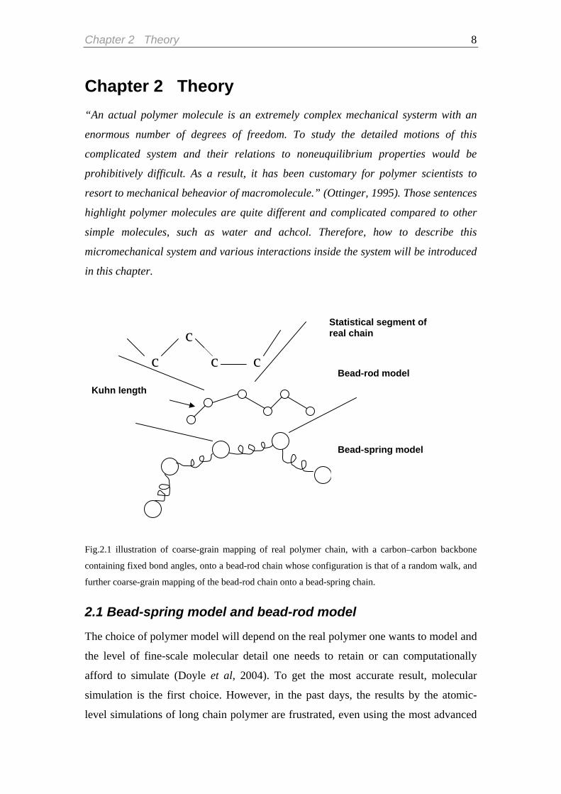
Fig.2.1 illustration of coarse-grain mapping of real polymer chain, with a carbon–carbon backbone
containing fixed bond angles, onto a bead-rod chain whose configuration is that of a random walk, and
further coarse-grain mapping of the bead-rod chain onto a bead-spring chain.
2.1 Bead-spring model and bead-rod model
The choice of polymer model will depend on the real polymer one wants to model and
the level of fine-scale molecular detail one needs to retain or can computationally
afford to simulate (Doyle et al, 2004). To get the most accurate result, molecular
simulation is the first choice. However, in the past days, the results by the atomic-
level simulations of long chain polymer are frustrated, even using the most advanced
c c
c c
Statistical segment of real chain
Bead-rod model
Kuhn length
Bead-spring model

Chapter 2 Theory 9
computer. Hence, it is needed to take a coarse-graining approximation in which we
only track the slow variables capturing the coarse-grain features and assume that in
the small scale, fast process remain at local equilibrium. Therefore, it is very
important to choose a proper level of coarse-graining in a given flow. The most
common coarse-grained models are the free jointed bead-rod and bead-spring models
shown in Figure 2.1
2.1.1. Bead-rod model In Kramer’s bead-rod model, a polymer chain is constructed by Nk beads connected
by Nk −1 rigid rods, which keep a constant length between each rod, corresponding to
Kuhn length bk (equal to the mean square end-to-end length of the bonds in a
statistical segment) shown in Figure 2.1.The beads serve to experience the drag force
given by the solvent molecules. As defined in this way, it can be seen that bead-rod
model is a discretized flexible chain with inextensible springs, whose flexibility can
be adjusted by changing the number of beads on a constant chain length. In other
words, the number of beads can be a parameter to control the internal freedom as well
as the discretization of the hydrodynamic drag force. But the chains do not experience
the excluded volume interaction between different chain segments (Hur et al, 2000).
Although it can give us an accurate description on polymers, the problem is that this
model is very computationally expensive due to the large number of dynamic
variables (bead positions) and rapid motion of the individual rods, which requires
smaller time steps. Therefore, we will use a model less demanding in computing
resources– Bead-spring model to capture the feature of the real polymer chains in our
project.
2.1.2. Bead-spring model A bead-spring chain is represented by N beads connected by Ns=N-1 entropic springs
shown in Figure 2.1. Each spring represents a large number of Kuhn steps Nk,s and
spring constant is dependent on the number of Kuhn length. If the molecular weight
increases, one can simply increase the number of Kuhn steps without wasting the
computing time on the increase of the number of the springs. From a physical aspect,
the springs do not represent the molecular interaction but entropic effects due to the
loss of more local degrees of freedom. The equilibrium length is zero between the
Chapter 2 Theory 10
successive beads. In addition, the model assumes that there is no excluded volume
interaction and hydrodynamic interaction between beads.
2.2 Physical phenomena in the model In these ranges of length scales (nm to µm) and time scales (µs to s), the following
effects are of primary importance for rheological properties (Larson, 2005):
(1) Viscous drag
(2) Entropic elasticity
(3) Brownian forces
(4) Hydrodynamics interaction
(5) Exclued-Volume (EV) interaction
(6) Entanglement
Those effects have been ordered based on their importance. Viscous drag is a kind of
frictional force exerted by surrounding solvent molecules, which is always important,
even under the weak flow strength. Entropic elasticity will become important when
the flow is strong enough to deform the configuration of polymer chains away from
their equilibrium states. Moreover, the Brownian motion, due to the collisions
between the polymer molecules and solvent molecules, will also influence the
distribution of the conformations. In addition to HI, it means that the subchain will
produce the disturbance to the flow field to influence the motion of other segments of
the chain. This effect will play an important role for polymers with longer chain. EV
interaction is the repulsive force which prevents two monomers to overlap, and will
make the chains tend to expand beyond the ideal random-walk conformations in
equilibrium. Fortunately, this interaction can be screened out in the good solvents at
their theta temperature. However, it could become important when the length scale
goes to the scale comparable to the radius of gyration of the chain. In addition to the
entanglement, since our target system is dilute solution of polymers, so the interchain
interaction can be neglected, which means we are focusing on the single molecule
dynamics.

Chapter 2 Theory 11
2.3 Equations for bead-spring model
Since the inertial force in the range of length scale of microdevices always can be
negligible, the force balance on each bead including drag force, spring force,
Brownian force leads to:
0drag s Bi i i+ + =F F F (2.1)
2.3.1. Drag force Hydrodynamic drag force is the Stokes drag acting on the beads. If we neglect the
hydrodynamic interaction and fluid inertia, it can be simplified as follows:
(2.2) ( (dragi i vζ= −F r& ))ir
Where ξ is the drag coefficient, r is the velocity of the ith bead and is the
undisturbed velocity field (namely the solvent velocity) at the position of bead i. For
simple shear flow, if the velocity at origin is zero, v(r
i ( )iv r
i)=κ · ri ,where κ is the transpose
of the velocity gradient tensor, κ=(∇ v)T. Substituting the Equation (2.2) into
Equation (2.1) yields:
(1 )s Bii i
ddt
κζ
= ⋅ + +r r F Fi (2.3)
This stochastic differential equation is the famous Langevin equation. The analytical
approach to this equation is beyond the scope of this project, a short introduction is
given in book (1995). 'Ottinger s&&
2.3.2. Spring force The effective spring force acting in the ith bead is given as
1 , 1sb i =F
si =F 1, 1sb sb
i i i N−− < <F F (2.4)
1,sbN i N−− =F
Where sbiF is the force that spring i acts on bead i.The spring force sb
iF is a function
of the extension Qi of spring i, where Qi= 1i+r - . Several force laws to describe the ir

Chapter 2 Theory 12
effective spring are commonly used .The simplest form is the linear force law-
Hookean law as follows:
(2.5) sbi H=F iQ
where H is the spring constant, which can be given as follows (Larson,2005):
2 22
,
32 ,2B s s
k s k
H k TN b
β β= = (2.6)
Figure 2.2 illustration of random coil stretched to its full length-contour length
However, a Hookean spring can be infinitely extended, which is unphysical. A more
realistic model should give an upper limitation of the extension-Ls= Nk,s bk, which is
the full extension of one segment of the chain represented by a single spring, ie. Ls=L/
Ns where L is the contour length of the chain as shown in Figure 2.2. For a freely
jointed chain, Kuhn and Gr n showed the spring force law by statistical mechanical
calculation as follows (Lasron, 2005):
u&&
1( iBi )
s S
k Tb L
−=QF L (2.7)
which is called inverse Langevin force law and the L is the Langevin function given
by coth 1/L θ θ= − (2.8)
where cothθ is the hyperbolic cotangent function . It can be seen that for the inverse
Langevin force law, the force increases linearly with the extension in the small
extension region; but grows rapidly for the large extension, especially the extension
goes to the maximum length of the spring..
However, Inverse Langevin force law is not often used. Several their approximation
forms are usually used in various analytical and numerical approaches. One of such
approximation is the Warner spring Law:
2Q1
sb ii
i
S
HF
L
=⎛ ⎞
− ⎜ ⎟⎝ ⎠
Q (2.9)
Random coilContour length L

Chapter 2 Theory 13
Q
Figure 2.3 illustration of FENE dumbbell model
The simplest Warner spring model is FENE(Finitely extensible nonlinear elastisc)
dumbbell, which incorporates non-linear effects into the Hookean dumbbell model
where two beads are connected by a linear spring as shown in Figure 2.3. The
maximum extension of the spring can be expressed as the dimensionless extensibility
parameter b as follows:
/ Bb HL k T= (2.10)
Where Ns=1, LS=L. So Nk,s in the FENE dumbbell model will be equal to the total
Kuhn steps Nk of the chain in bead-rod model. Combining Equation (2.6) and (2.10),
it leads to:
,( 1)k s kb N b= − (2.11)
A more accurate approximation, namely Cohen Padé approximation can be given as
follows (Larson,2005) :
2
2
3[
3 1
i
Ssb ii
i
S
QLHF
QL
⎛ ⎞− ⎜ ⎟⎝ ⎠=⎛ ⎞− ⎜ ⎟⎝ ⎠
Q ] (2.12)
which is much closer to the Inverse Langevin force law. Since DNA and many other biopolymers have helical structures along the backbones,
they are bendable but difficult to experience large torsional bond rotations.
Yamakawa in 1979 established the wormlike chain model for this kind of polymer.
By statistical mechanics calculations, this model leads to the approximate force law,
namely Marko-Siggia spring law as follows (Larson, 2005):
2 2
1 1 2 1 1[ 1 ] [ 14 4 3 4 4
sb i i iBi S
p S S S
Q Q Q Qk TF HLL L Lλ
− −⎛ ⎞ ⎛ ⎞
= − − + = − − +⎜ ⎟ ⎜ ⎟⎝ ⎠ ⎝ ⎠
]i
SL (2.13)
where Pλ is the persistence length and Kuhn length bk =2 Pλ .The spring constant is
the same with the coefficient before. Since we have introduced those spring force law,
the comparison of difference force law is presented in Figure 2.4.

Chapter 2 Theory 14
It is important to note that various force laws in the bead spring model is derived by
the equilibrium statistical properties, so it would raise a subtle problem when using
the bead spring model in flow or nonequilibrium situation. Therefore, it is implicitly
assumed that the springs are deformed slowly enough in such cases, so that its
configuration space can be fully sampled. In a sense, we assume that a local
equilibrium has been created in the phase space (Doyle et al, 2004).
Figure 2.4 Comparison of different spring force law vs normalized molecule extension. The normalized
extension is the distance between a bead and its successive bead divided by the maximum spring length.

Chapter 2 Theory 15
2.3.3. Brownian force
Figure 2.5 illustration of a set random number with zero mean value uniformly distributed in [-1,1] (A) and its
histogram(B)
B A
Although macromolecules have longer chain than small molecules, but they are small
enough that Brownian kicks from the solvent molecules will change the positions and
configurations rapidly. The characteristic time of this Brownian kicks is much smaller
than the relaxation time of the polymer chain but this Brownian influence from the
solvent is large enough to be treated as a kind of stochastic, random force (Schiek et
al ,1997). Thus, the Brownian force over a time scale dt can be given by
1/ 26( )B Bk Tt
dtζ⎛ ⎞= ⎜ ⎟
⎝ ⎠F (2.14)
where n is a random three dimensional vector ,each component of which is random
number uniformly distributed between [-1,1] as shown in Figure 2.5. The factors of
kBT and ζ come out due to the fluctuation-dissipation theorem, which bridges up
Brownian force with drag force (Larson, 2005). A general form of the fluctuation-
dissipation theorem in three dimensions is represented by
( )
( ) 0
( ) ( )
B
B B
t
t t A t tδ
=
′ ′= −
F
F F (2.15)
Where δ (t- ) is the delta function, when t goes to t′ very close to 0, δ (t- ).and A is
a constant needed to be determined. Let’s suppose a particle moves in a viscous
solvent and only influenced by the random force from the solvent, the equation of
motion can be expressed as following way:
t′ t′
( )Bd t
dtζ =
r F (2.16)

Chapter 2 Theory 16
so the mean square displacement at given time t can be got from:
21 1 2 22 0 0
1( ) (0) ( ) ( )t tB Bt F t dt F
ζ− = ⋅∫ ∫r r t dt (2.17)
Which can be simplified to :
21 2 1 22 0 0
1( ) (0) ( ) ( )t t B Bt dt dt F t
ζ− = ⋅∫ ∫r r F t (2.18)
with Equation (2.15)
21 1 2 2 12 20 0 0
1( ) (0) ( )t t tAt dt A t t dt Adδ 2
At tζ ζ ζ
− = − = =∫ ∫ ∫r r (2.19)
In addition, the mean square displacement of particle is also satisfied with the Einstein equation: 2( ) (0) 6t − =r r Dt (2.20)
Thus, it leads to the analytical form of A:
2 266 BB
k TA D k T6ζ ζ ζζ
= = = (2.21)
Therefore, the random force can be expressed as follows:
[ ] [1/ 2 1/ 2
( ) ( ) 6 ( )
6 ( ) 6 /
B BB
BB B
t t k T t t
k T t t k T dt
ζ
ζ ζ
′ ′= −
′= − =
F F δ
F δ ] (2.22)
In the simulation, we will keep the time step constant and n is a random three
dimensional vector ,each component of which is random number uniformly
distributed between [-1,1]. In this way, we can not only mediate the magnitude of the
random force, but also randomize the direction of the force. Therefore, the equation of
motion only with Brownian force can be expressed as the following way based on
Equation (2.16) and (2.22):
1/ 2 1/ 26 6i Bd k T
dt dt dtζ⎛ ⎞ ⎛ ⎞= ⋅ =⎜ ⎟ ⎜ ⎟
⎝ ⎠⎝ ⎠
r Dn ⋅n (2.23)
where D is actually a 3x3 symmetric tensor, therefore, it should be at least a semi-
definite tensor. We will discuss this issue in details in the next section.Substituting
Equation (2.14) into Equation (2.1), it leads to the simplest form of Langevin equation
for bead-spring model as follows:
1/ 2
61 si Bi i
d k Tdt dt
κζ ζ
⎛ ⎞= ⋅ + + ⎜ ⎟
⎝ ⎠
r r F in (2.24)
or
1/ 2
61( ) ( ) ( ) s Bi i i i
k Tdtt t t t dtκζ ζ
⎛ ⎞ ⎛+ ∆ = + ⋅ + +⎜ ⎟ ⎜
⎝ ⎠ ⎝r r r F i
⎞⎟⎠
n (2.25)

Chapter 2 Theory 17
This stochastic equation will govern the probability distribution of the configuration
and position of the segments of the chain in the confined geometry. One needs to
integrate this equation forward in time. The Brownian term will lead to many
independent trajectories. By averaging them together, we can get the ensemble-
averaged properties based on the time-evolution. Therefore, repetition of producing
the independent trajectories is a time-consuming but necessary part of the simulation.
After getting the time-averaged properties, it can be assumed as the steady state
properties of molecules according to ergodic hypothesis (Doyle et al,2004).
2.3.4. Hydrodynamic interaction
Figure 2.6 Movement of particle 1 generates the motion of solvent molecules, which eases the motion
of particle 2 in the same direction.
solvent 1
2
Motion of solvent molecules
Many practical applications in dilute polymer solutions are subject to hydrodynamic
interaction (HI), such as gel permeation chromatography and the flow of biological
fluids in the living systems. The important physical feature is that in a low Reynolds
number flow, the hydrodynamic interaction due to a point force or boundary falls
relatively slowly with the increasing distance. It becomes very important, especially if
the length scale of the system is comparable to the characteristic length scale of
polymers. In this section, three models with different levels to treat HI effects are
introduced: Free-draining model (without HI effect), Bulk HI model (bead-bead
interaction),Full HI model (Bulk HI+ wall hydrodynamic effect)
I. Hydrodynamic interaction in a free solution (Bulk HI model) The concept of hydrodynamic interaction is the motion of a segment will produce a
disturbance to the velocity field in the flow due to the point force at this point, which
will influence the motion of the entire chain accordingly shown in Figure 2.6. If the
force is weak enough, the disturbance created by this force at rdragjF j to the velocity
Chapter 2 Theory 18
field at position ri of bead i can be approximated by a linear function of the
hydrodynamic drag force as follows: dragj−F
(2.26) (drag s Bi ij j ij j′ = − ⋅ = ⋅ +v Ω F Ω F F )j
where is the hydrodynamic interaction tensor or mobility tensor, which is the
function of the displacement of r
ijΩ
i-rj between the bead i and j. If we incorporate this
effect into Largevin equation, the following stochastic equation can be get:
1/ 2
1 1 1
6N N Nij si
i ij jj j jj B
ddt k T dt
κ= = =
∂ ⎛ ⎞= ⋅ + ⋅ + ⋅ + ⋅⎜ ⎟∂ ⎝ ⎠∑ ∑ ∑
Dr r D F Br ij jn (2.27)
where Dij is the diffusion tensor and tensor Bij can be represented as follows according
to Eq (2.23):
1
N
ij il ljl=
= ⋅∑D B B (2.28)
If Equation (2.28) is statisfied, a Cholesky decompostion can made between Dij and Bij
as follows 1(Hsieh et al, 2005):
1/ 21
2
1
1/ 21
1 ,
0,
B D B
D B BB
BB
α
αα αα αγγ
β
αα αγ βγγ
αβββ
αβ
α β
α β
−
=
−
=
⎛ ⎞= −⎜ ⎟⎝ ⎠
⎛ ⎞−⎜ ⎟
⎝ ⎠=
= <
∑
∑> (2.29)
Here , ,α β γ are the row and column positions of the elements in the tensor D and B.
Here the diffusion tensors are supposed to be symmetric, positive-definite. However,
this may be not the case during the simulation. This problem has its physical origin:
on one hand, we assumed point particles or beads with zero radius during the
derivation of Oseen-Burgers tensor; on the other hand, when calculating the frication
coefficient for the given solvent, we implicitly assumed a bead radius a given by
Stokes law 6 aζ πη= . Hence, Oseen-Burgers tensor only can lead to realistic results
for the bead separation comparable to 2a (Ottinger et al, 1995)2.Therefore, an
alternative approach- Chebyshev polynomial approximation is introduced in the
appendix A-2.
1 Please refer Cholesky decomposition in appendix for details 2 Please refer this part Appendix: A-3
Chapter 2 Theory 19
For the diffusion tensor D, which is 3×3 block components of 3N×3N diffusion
tensor, there are several forms in use. Mathematically, a Green function represents the
influence of a bead being moved through the solution. The simplest one is the Oseen-
Burgers tensor , which assumes that the beads can be regarded as point sources
of drag in the solvent:
OBΩ
1(6ij B ij ij
s
k Ta
δπη
=D I Ω )+
Ω
(2.30)
(2.31) (1 ) OBij ij ijδ= −Ω
2
( )( )18ij
i j i jOB
S i j i jπη
⎡ ⎤− −⎢ ⎥= +⎢ ⎥− −⎣ ⎦
r r r rΩ I
r r r r (2.32)
Where I is a unit tensor, δij is the Kronecker delata and - is the separation vector
between the ith and jth beads. However, Oseen-Burgers tensor is not suitable for
Brownian dynamics simulation, because it will become nonpositive when - is
comparable to or less than the bead radius as we mentioned before. Here is the
observation point to see the velocity perturbation due to the point force at where
is the source point. Therefore, the perturbation to the flow field at any point is the
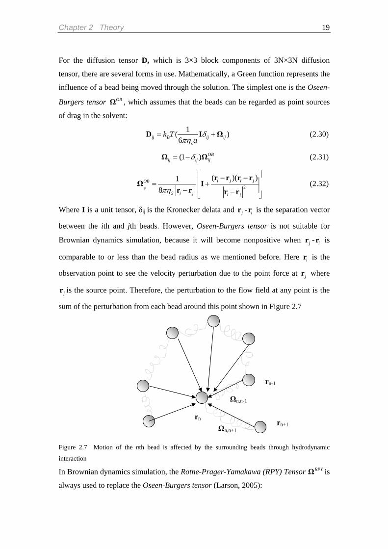
sum of the perturbation from each bead around this point shown in Figure 2.7
jr ir
jr ir
ir
jr
jr
rn-1
Ωn,n-1
rn rn+1Ωn,n+1
Figure 2.7 Motion of the nth bead is affected by the surrounding beads through hydrodynamic
interaction
In Brownian dynamics simulation, the Rotne-Prager-Yamakawa (RPY) Tensor RPYΩ is
always used to replace the Oseen-Burgers tensor (Larson, 2005):

Chapter 2 Theory 20
1 2 2
( )( )1 , 28ij
i j i jRPYi j
S i j i j
C C forπη
⎡ ⎤− −⎢ ⎥= + −⎢ ⎥− −⎣ ⎦
r r r rΩ I r
r r r ra≥r (2.33)
1 2 2
( )( )1 , 26ij
i j i jRPYi j
S i j
C C foraπη
⎡ ⎤− −⎢ ⎥′ ′= + −⎢ ⎥−⎣ ⎦
r r r rΩ I r
r ra<r (2.34)
2
1 2
2
2 2
213
21
j
j
aC
aC
= +−
= −−
r r
r r
(2.35)
1
2
91
323
32
j
j
Ca
Ca
−′ = −
−′ =
r r
r r (2.36)
Here the first expression indicates the beads are well separated and the second means
the beads have some overlaps with each other. However, it seems that the second case
doesn’t happen frequently in the simulation due to the excluded volume effect.
For Oseen tensor and RPY tensor, Ωij=0 for i=j, and 0ijj∂ ∂ ⋅ =r Ω for all i, j in the
free solution, things will be different in the confined geometry. Those modifications
will be discussed in the next section.
The strength of HI effects between beads can be evaluated by the following
parameters:
( )
1/ 2*
3 1/ 23
336 12s sB s s
HhRk T R
ζ ζη ππ π η
⎛ ⎞= = =⎜ ⎟
⎝ ⎠
ζ (2.37)
where is the elastic constant of the spring and 23 /B SH k T R= ,s k KR b N= S is the
root-mean-square end-to-end vector of a spring at equilibrium. Based on this
definition, Equation (2.33)-(2.34) can be rewritten as follows:
6
Bii
S
k Taπη
=D I (2.38)
Chapter 2 Theory 21
*
1 2 2
( )( )3 , 28ij
si j i jRPY B
i jS i j i j
h Rk T C C fora
π
πη
⎡ ⎤− −⎢ ⎥= +⎢ ⎥− −⎣ ⎦
r r r rD I
r r r ra− ≥r r (2.39)
*
1 2 2
( )( )3 , 26ij
si j i jRPY B
i jS i j
h Rk T C C fora a
π
πη
⎡ ⎤− −⎢ ⎥′ ′= +⎢ ⎥−⎣ ⎦
r r r rD I
r ra− <r r (2.40)
It can be seen that the HI effect will be different due to the different choices of bead
radius, which will make simulation result far from the experimental data. Therefore,
when the simulation is carried out, the hydrodynamic interaction parameter could be
another parameter to optimise.
II. Hydrodynamic interaction in a confined geometry (Full HI model) Traditionally, people treat the HI effect to the level of bead-bead(which is named
Bulk HI model in the above section), but the effect between the wall and bead comes
into play in the confined geometry, especially when we have lowered down to a
length scale comparable to the radius of gyration of the polymer. How to treat the
hydrodynamic interaction and into which level? It is a critical point for us to explain
dynamics of the biomolecules in the microchannel, because the Green function for
hydrodynamic interaction is highly dependent on the geometry of the channel. In
addition, the analytical solution only exists in few special cases, which are needed to
be highly symmetric geometry. Here we introduced the method proposed by
Jendrejack et al (2004) to evaluate the HI effect on a more accurate level, which is
called Full HI model.
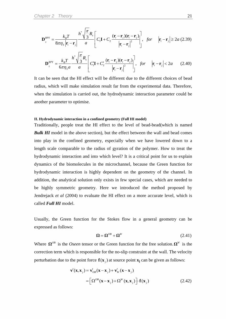
Usually, the Green function for the Stokes flow in a general geometry can be
expressed as follows:
OB W= +Ω Ω Ω (2.41)
Where is the Oseen tensor or the Green function for the free solution. is the
correction term which is responsible for the no-slip constraint at the wall. The velocity
perturbation due to the point force at source point x
OBΩ WΩ
( )jf x j can be given as follows:
( , ) ( ) ( )j OB j W′ ′ ′= − + −v x x v x x v x x j
j⎤⎦
(2.42) ( ) ( , ) ( )OB Wj j⎡= Ω − +Ω ⋅⎣ x x x x f x

Chapter 2 Theory 22
Since the Stokes equations are linear and homogeneous, the velocity produced by
different forces and boundaries at the different points in the liquids are additive.
Therefore, the velocity perturbation ( ),w i j′v x x can be get by the solving the classical
incompressible Navier- Stokes flow problem:
2 0,s Wp η ′−∇ + ∇ =v 0W′∇ ⋅ =v (2.43)
With the boundary condition: 0OB W′ ′+ =v v at the wall (2.44)
Thus, the boundary condition becomes W OB′ ′= −v v , which means ( , )wi j =Ω x x
. Because we always use the RPY tensor instead of the Oseen Tensor,
we should substitute Equation (2.33) into the boundary condition, then we would find
the explicit velocity for the boundary.
(OBi j− −Ω x x )
Using this boundary condition and point force f1 acting on the direction 1, this Stokes
flow problem can be solved by finite element method (Jendrejack et al, 2004). Here
we used the FEMLAB finite element software package(Comosol) to solve this
classical fluid dynamic problem. After we get the velocity perturbation for the wall,
the first column of the could be given as the following way: ( , )wi jΩ x x
11
211
31
1W
WW
Wf
⎛ ⎞Ω⎜ ⎟
′Ω =⎜ ⎟⎜ ⎟Ω⎝ ⎠
v (2.45)
Where 1,2,3 represents the three directions. The second and third column of the
can be got in the similar way by applying the point forces in the direction
of 2 and 3, respectively. Since we have the Green function for wall, the total
Green function can be expressed as following way:
( , )wi jΩ x x
( , )wi jΩ r r
(2.46) (1 ) ( ) ( , )OB Wij ij i j i jδ= − − +Ω Ω r r Ω r r
Compared to the flow of the free solution, is nonzero and ijΩ 0ijj∂ ∂ ⋅ ≠r Ω for i=j, which will lead to a nonzero drift term in Equation (2.27). The Green’s function is evaluated on the grids before the Brownian simulation, which
means we will make those grid data into a lookup table for a given geometry. During
the simulation, Green’s function and its divergence will be evaluated by the finite
interpolation (please refer the detail in Appendix A-2).

Chapter 2 Theory 23
From equation (2.32) and (2.33), it can be seen that the hydrodynamic interaction
between beads decays relatively fast as 1/r2 .For a particle close to the wall, it falls off
with the distance to the point force as 1/r (Jendrejack et al, 2004), which means even
the beads are far from the wall, the effect from the wall still exists beyond the range of
excluded volume interaction from we will introduced in section 2.3.6. It indicates that
hydrodynamic coupling to bounding surfaces could influence molecule’s motions to a
greater extent and over a longer range (Dufresne et al, 2000).
Appendix: Cholesky Decomposition Suppose we have a symmetric and positive definite matrix3 or semi-positive
definite matirx. It can be efficiently decomposed into lower and upper triangular
matrix as follows:
11 1 11 11 1
1 1
0
0
n n
m mn n nn
a a l l
a a l l
l
l
⎛ ⎞ ⎛ ⎞⎛⎜ ⎟ ⎜ ⎟⎜=⎜ ⎟ ⎜ ⎟⎜⎜ ⎟ ⎜ ⎟⎜⎝ ⎠ ⎝ ⎠⎝
K L L
M O M M O M M O M
L L L nn
⎞⎟⎟⎟⎠
the elements of the upper and lower triangular matrix can be get as follows:
( )
211 11 11 11
21 21 11 21 21 11 1 1 11
1/ 22 2 222 21 22 22 22 21
/ , , /n n
a l l aa l l l a l l a l
a l l l a l
= → =
= → = =
= + → = −
L
we can also give a general form of the solution:
(2.47) 1/ 21
2
1
i
ii ii ikk
l a l−
=
⎛= −⎜⎝ ⎠
∑ ⎞⎟
l⎟
(2.48) 1
1
/j
ij ij jk ik iik
l a l l−
=
⎛ ⎞= −⎜⎝ ⎠
∑
3 A symmetric matrix is positive definite if all the eigenvalues are positive.
Chapter 2 Theory 24
2.3.5. Excluded Volume Effect
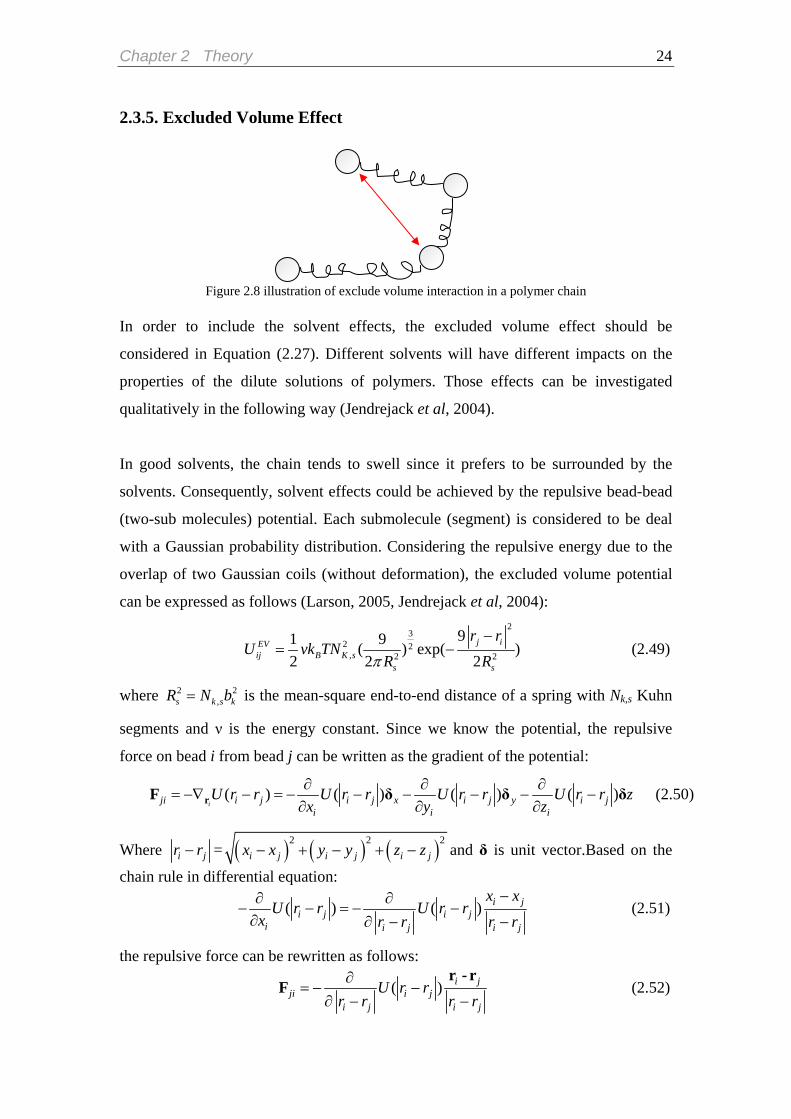
Figure 2.8 illustration of exclude volume interaction in a polymer chain
In order to include the solvent effects, the excluded volume effect should be
considered in Equation (2.27). Different solvents will have different impacts on the
properties of the dilute solutions of polymers. Those effects can be investigated
qualitatively in the following way (Jendrejack et al, 2004).
In good solvents, the chain tends to swell since it prefers to be surrounded by the
solvents. Consequently, solvent effects could be achieved by the repulsive bead-bead
(two-sub molecules) potential. Each submolecule (segment) is considered to be deal
with a Gaussian probability distribution. Considering the repulsive energy due to the
overlap of two Gaussian coils (without deformation), the excluded volume potential
can be expressed as follows (Larson, 2005, Jendrejack et al, 2004):
2
32 2
, 2
91 9( ) exp( )2 2 2
j iEVij B K s
s s
r rU vk TN
Rπ−
= 2R−
2
(2.49)
where 2,s k s kR N b= is the mean-square end-to-end distance of a spring with Nk,s Kuhn
segments and ν is the energy constant. Since we know the potential, the repulsive
force on bead i from bead j can be written as the gradient of the potential:
( ) ( ) ( ) ( )iji i j i j x i j y i j
i i iU r r U r r U r r U r r z
x y z∂ ∂ ∂
= −∇ − = − − − − − −∂ ∂ ∂rF δ δ δ (2.50)
Where i jr r− = ( ) ( ) ( )2 2i j i j i j
2x x y y z z− + − + − and δ is unit vector.Based on the
chain rule in differential equation:
( ) ( ) ii j i j
i i j i j
jx xU r r U r r
x r r r r−∂ ∂
− − = − −∂ ∂ − −
(2.51)
the repulsive force can be rewritten as follows:
( ) i jji i j
i j i j
U r rr r r r∂
= − −∂ − −
r - rF (2.52)
Chapter 2 Theory 25
Some other potential, such as Lennard-Jones, soft potential are also commonly used in
the Brownian simulation. However, it is not obvious how the parameters in those
models adjust with the molecule discretization Nk,s. That’s the reason why they
developed such kind of potential (Jendrejack, 2003).
In the theta solvents, polymer molecule can’t distinguish the polymer and solvent at
larger length scale, which means polymers can’t feel ‘itself’. The theta effects can be
simply realized by removing the potential. In a bad solvent, polymer tends to contract,
which means polymer prefer to get together, which can be achieved by adding an
attractive bead-bead potential.
2.3.6. Physical confinement
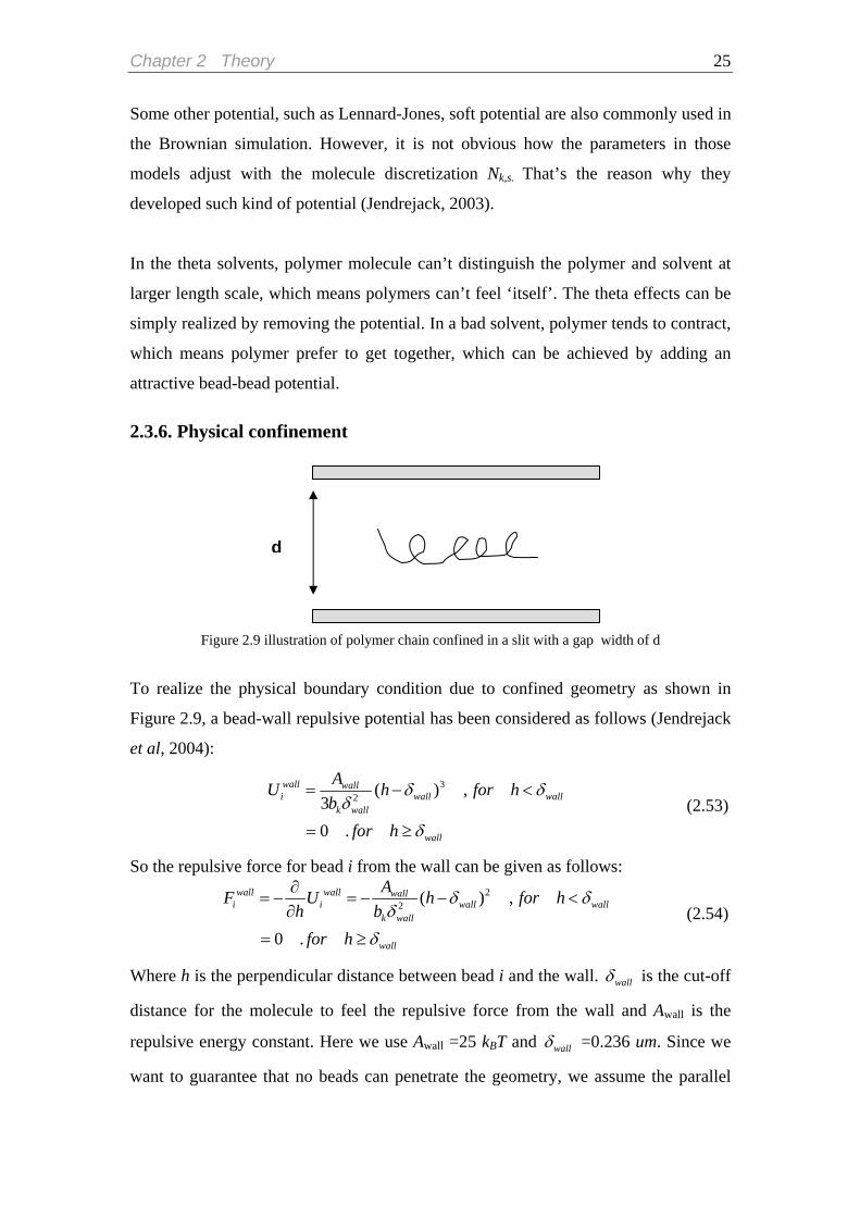
Figure 2.9 illustration of polymer chain confined in a slit with a gap width of d
d
To realize the physical boundary condition due to confined geometry as shown in
Figure 2.9, a bead-wall repulsive potential has been considered as follows (Jendrejack
et al, 2004):
3
2 ( ) ,30 .
wall walli wall wall
k wall
wall
AU h for hb
for h
δ δδ
δ
= − <
= ≥ (2.53)
So the repulsive force for bead i from the wall can be given as follows:
2
2 ( ) ,
0 .
wall wall walli i wall wall
k wall
wall
AF U h for hh b
for h
δ δδ
δ
∂= − = − − <
∂
= ≥ (2.54)
Where h is the perpendicular distance between bead i and the wall. wallδ is the cut-off
distance for the molecule to feel the repulsive force from the wall and Awall is the
repulsive energy constant. Here we use Awall =25 kBT and wallδ =0.236 um. Since we
want to guarantee that no beads can penetrate the geometry, we assume the parallel

Chapter 2 Theory 26
walls are perfect elastic. During the process, if bead is the outside the wall, the wall
can reflect the bead back into the same depth without affecting the bead displacement
in the direction parallel to the wall. From above statement, it can be seen that the
repulsive force from the wall is a short-range influence (the effective region is 0.236
um) compared with the long-range hydrodynamic interaction.
Reference Doyle, P.S. and Underhill, P.T., Brownian dynamics simulations of polymers and soft matter, In S. Yip,
editor, Handbook of Materials Modeling, volume I. Kluwer Academic Publishers, 2004.
J S.Hur,E S G.Shaqfeh,R G.Larson Brownian dynamics simulations of DNA molecules in shear flow,
J.Rheol.44,713-742,2000.
R.G.Larson, The rheology of dilute solutions of flexible polymers: Progress and problems, J.Rheol.49
(1), 1-70, 2005
Ottinger,H.C., Stochastic Process in Polymeric Liquids, Springer,Berlin,1995
C.C.Hsieh, L.Li,R. G.Larson, Modeling hydrodynamic interaction in Brownian dynamics: simulations
of extensional flows of dilute solutions of DNA and polystyrene’, J.Non-Newtonian Fluid
Mech.113,147-191,2003
R.M.Jendrejack, D.C.Schwartz, J.J.de Pablo, M.D.Graham, Shear-induced migration in flowing
polymer solutions: simulation of long-chain DNA in microchannels, J.Chem Phys,120,2513-2529,2004
R.M.Jendrejack, Multiscale Simulations of Dilute-Solution Macromolecular Dynamics in Macroscopic and Microscopic Geometries, Doctoral dissertation, 2003 COMSOL AB Sweden, FEMLAB 3.0,http://www.femlab.com
E.R. Dufresne, T.M. Squires, M.P.Brenner, Hydrodynamic Coupling of Two Brownian Spheres to a
Planar Surface, Phys. Rev. Lett. 85, 3317,2000
R.L. Schiek, E.S.G.Shaqfeh, Cross-stream line migration of slender Brownian fibres in plane
Poiseuille flow, J.Fluid Mech., 332, 1997

Chapter 3 Numerical Scheme 27
Chapter 3 Numerical Scheme Since the starting point the stochastic differential equation has been developed in
the last chapter, we must integrate the equation forward in time in order to get the
trajectories of the molecule. Two most common integration schemes for FENE
dumbbell and Bead-spring model are introduced in this chapter.
3.1 Simulation scheme4
3.1.1. Explicit Euler Scheme
Figure 3.1 illustration of the position vector ri, end-to-end vector R,center of mass rc, radius of gyration
RG in bead-spring model
The governing equation is given as Eq(2.25) as follows:
1/ 261( ) ( ) ( ) s B
i i i ik Tdtt t t t dt
ζ ζ⎛ ⎞ ⎛
+ = + ⋅ + +⎜ ⎟ ⎜⎝ ⎠ ⎝
r r κ r F i⎞⎟⎠
n
1
To integrate this equation, the simplest scheme is the explicit Euler scheme. By
marching the time, we can update the position of beads. In addition, the trajectories of
the connector vector Qi (t), center of mass rc(t) and the radius of gyration RG(t)
shown in Figure 3.1 can be given as follows:
1i i i+ += −Q r r (3.1)
1
1 N
ciN =
= i∑r r (3.2)
2
1
1 (N
G iiN =
= −∑R r )cr
Substituting Equation (2.4) into Equation (2.25) leads to:
(3.3)
4 To illustrate the scheme, Free draining model is taken as the example for simplicity
r0
r1
r2
rn-1
rn
end-to-end
Q1 RG
vector R rc
Qn
Chapter 3 Numerical Scheme 28
1/ 2
1 161 s Bk Tdt⎛ ⎞ ⎛ ⎞ ( ) ( ) , 1i it t dt i
ζ ζ+ ⋅ + + =⎜ ⎟ ⎜ ⎟⎝ ⎠ ⎝ ⎠
r κ r F n
1/ 2
161( ) ( ) ( ) ,1sb sb B
i i i i ik Tdtt t dt i
ζ ζ−
⎛ ⎞ ⎛ ⎞+ ⋅ + − + < <⎜ ⎟ ⎜ ⎟⎝ ⎠ ⎝ ⎠
r κ r F F n( )i t t+ =r N (3.4)
1/ 2
161( ) ( ) ,sb B
N N N ik Tdtt t dt i
ζ ζ−
⎛ ⎞ ⎛ ⎞+ ⋅ − + =⎜ ⎟ ⎜ ⎟⎝ ⎠ ⎝ ⎠
r κ r F n N
If we take FENE dumbbell model for example, equation (3.4) for two beads becomes
⎛ ⎞1/ 2
11 1 1 12
1
61 ( ) ( ) ( ) , 1Q1
B
s
H k Tdtt t t t dt i
L
ζ ζ
⎜ ⎟⎛ ⎞⎜ ⎟+ = + ⋅ + + =⎜ ⎟⎜ ⎟ ⎝ ⎠⎛ ⎞⎜ ⎟− ⎜ ⎟⎜ ⎟⎝ ⎠⎝ ⎠
Qr r κ r n (3.5)
1/ 2
12 2 2 22
1
61 ( ) ( ) ( ) ,Q1
B
s
H k Tdtt t t t dt i
L
ζ ζ
⎛ ⎞⎜ ⎟
⎛ ⎞⎜ ⎟+ = + ⋅ − + =⎜ ⎟⎜ ⎟ ⎝ ⎠⎛ ⎞⎜ ⎟− ⎜ ⎟⎜ ⎟⎝ ⎠⎝ ⎠
Qr r κ r n 1 (3.6)
Those equations can be decoupled into three components x,y,z, take Equation (3.5) in
simple shear flow for example:
1/ 21,
1, 1, 1, 1,2
1
61 ( ) ( ) ( )
1
x Bx x x
s
HQ k Tdtr t t r t r t dt nQL
γζ ζ
⎛ ⎞⎜ ⎟
⎛ ⎞⎜ ⎟+ = + + + ⎜ ⎟⎜ ⎟ ⎝ ⎠⎛ ⎞⎜ ⎟− ⎜ ⎟⎜ ⎟⎝ ⎠⎝ ⎠
& x
1/ 2
1,1, 1, 1,2
1
61 ( ) ( )
1
y By y
s
HQ k Tdtr t t r t dt nQL
ζ ζ⎛ ⎞
+ = + + ⎜ ⎟⎝ ⎠⎛ ⎞
− ⎜ ⎟⎝ ⎠
y (3.7)
1/ 2
1,1, 1, 1,2
1
61 ( ) ( )
1
z Bz z
s
HQ k Tdtr t t r t dt nQL
ζ ζ⎛ ⎞
+ = + + ⎜ ⎟⎝ ⎠⎛ ⎞
− ⎜ ⎟⎝ ⎠
z
By updating the time, we can update the bead position in three directions, and then
owever, we have to choose the small time step t =10-4-10−5s for explicit Euler
collect the molecular configurations by Equation (3.1)-(3.3).
H
method (we will discuss the choice of parameters later). If the time step is larger than
that, the maximum extension length would be larger than the contour length of the

Chapter 3 Numerical Scheme 29
chain, which is unphysical. Since the use of random variables in the simulation and a
finite number of trajectories in the ensemble, there will be intrinsic statistical noise to
the method. According to the theory of statistics, the magnitude of this error is
proportional to N-1/2T where NT is the number if they are independent trajectories.
(Doyle et al 2004)
3.1.2. Predictor-Corrector Method er scheme and its relatively high error,
up
Due to the weak convergence of the Eul
O&& ttinger (1995) developed a more efficient second-order algorithm developed by
dating the dumbbell trajectories of connector vector first. If we take differences
between Equation (2.25) with successive indices i for FENE dumbbell model, we can
get the equations as follows:
predictor:
1/ 2
11 1 1 12
1
62 ( ) ( ) ( ) (Q1
B
s
H k Tdtt t t t dt
L
ζ ζ
⎛ ⎞⎜ ⎟
⎛ ⎞⎜ ⎟+ = + ⋅ − + −⎜ ⎟⎜ ⎟ ⎝ ⎠⎛ ⎞⎜ ⎟− ⎜ ⎟⎜ ⎟⎝ ⎠⎝ ⎠
QQ Q κ Q n 2 )n (3.8)
Where 1 ( )t t+Q is the predictor , here we use the value from explicit Euler method
redictor. as the p
corrector:
1 11 1 1 1 2 2
1 1
1/ 2
1 2
( )2 ( ) ( ) 0.5 [ ( ) ( )] [ ]Q ( )1 1
6 ( )
s s
B
t tHt t t t t t dtt t
L L
k Tdt
ζ
ζ
⎛ ⎞⎜ ⎟
+⎜ ⎟+ = + ⋅ + + − +⎜ ⎟⎛ ⎞ ⎛ ⎞+⎜ ⎟− −⎜ ⎟ ⎜ ⎟⎜ ⎟⎝ ⎠ ⎝ ⎠⎝ ⎠
⎛ ⎞+ −⎜ ⎟⎝ ⎠
Q QQ Q κ Q QQ
n n
(3.9)
Equation (3.9) also can be decoupled into three directions in Cartesian coordinates. If
we take the combination of Equation (2.25) and successive index i, then time
evolution of the center of mass can be get: 1/ 2 2
1
6 1 ( ) ( ) ( ) ,2
Bc c c
i
k Tdtt t t t dtξ =
⎛ ⎞+ = + ⋅ + ⎜ ⎟
⎝ ⎠i∑r r κ r n (3.10)
Chapter 3 Numerical Scheme 30
Based on Equation(3.9) and Equation(3.10), we can get the trajectories of the internal
connectors Qi(t) and the center of mass position vector rc, because we know the
relationships between Qi(t), rc, and ri(t) as follows:
11
1 ( ) ( ) ( ) ( ) ( )2
N
c j cj
N jt t t tN=
−= − = −∑r r Q r Q j t
j t
(3.11)
(3.12) 1
1 11
( ) ( ) ( ) ( ) ( )i
i jj
t t t t−
=
= + = +∑r r Q r Q
Compared to explicit Euler method, predictor-corrector method don’t have good
performance on increasing speed on each step, but it saves computing time by
increasing the step size, since this method can prevent the molecular extension beyond
the maximal length efficiently.
3.2 Dimensionless parameter For FENE dumbbell model, we scale the length with /Bk T H and the time with Fτ ,
where Fτ is the characteristic time of FENE dumbbell and we assume it is the
relaxation time of molecular stretch (defined in chapter 4). In order to characterize the
flow strength, the Weissenberg number is defined as follows, which indicates the
chain relaxation time scale relative to the characteristic flow time scale:
FWi γτ= & (3.13)
where γ& is shear rate.In Bead-spring model, the characteristic time and length is the
relaxation time τ of molecular stretch (defined in chapter 4) and Kuhn length bk
respectively. Therefore, Weissenberg number for Bead-spring model can be defined
as follows:
Wi γτ= & (3.14)
3.3 Pseudo random number generator In our simulation, it is needed to generate a large number of random numbers, which
is the stochastic origin of the equation. At first, we used the build-in function
random_number ( ) in FORTRAN. When we tried to optimize the code to reduce
computational time, we found the build-in function almost uses most of the time,

Chapter 3 Numerical Scheme 31
which is very time-expensive. Therefore, it would be a good idea to code the random
number generator by ourselves.
System-supplied random number generators are always linear congruential
generators, which generate a sequence of integers I1,I2,I3,…,each between 0 and m-
1(a large number) by the recurrence relation as follows:
1j jI aI c+ = + (3.15)
then get the modulus based on m as follows: 1mod( , )jv I + m= (3.16)
then divided by m /U v m= (3.17)
Where a and c are positive integers called the multiplier and increment respectively. If
m, a, c are properly chosen and repeating this recurrence relation over a period, all
possible numbers U between 0 and 1 will occur at some point.
Here we will take random number generator proposed by Lewis, Goodman and Miller
in 1969, which has passed almost all the theoretical tests in the past years (Press et al
,1992). Here are their parameters for the random number generator:
(3.18) 5 217 16807 0 2 1 2147483647a c m= = = = − =
Implementing the algorithm (3.16)-(3.18), a sequence of random number uniformly
distributed in [0, 1] can be generated. To get a sequence of random number uniformly
distributed in [-1,1], the algorithm need to be modified as follows:
1 2 /U v m= − + × (3.19)
After tested, this random number generator reduces half of the total time compared
with that by build-in function in FORTRAN.

Chapter 3 Numerical Scheme 32
Reference
Doyle, P.S. and Underhill, P.T. Brownian dynamics simulations of polymers and soft matter, In S. Yip,
editor, Handbook of Materials Modeling, volume I. Kluwer Academic Publishers, 2004.
Ottinger,H.C., Stochastic Process in Polymeric Liquids, Springer,Berlin,1995
I.Ghosh,G H.Mckinley, R A.Brown,R C.Armstrong, Deficiencies of FENE dumbell models in
describing the rapid strenching of dilute polymer solutions,.J.Rheol.45,721-758, 2001.
W.H.Press, S.A. Teukolsky, William T. Vetterling, B. P. Flannery, NUMERICAL RECIPES IN
FORTRAN 77: THE ART OF SCIENTIFIC COMPUTING, Cambridge University Press, 1992

Chapter 4 Choices of parameter 33
Chapter 4 Choices of parameter Since the local physicochemical properties along polymer chains are not that
important, bead-rod model and bead spring model is enough to capture some critical
non-linear properties of polymer chains. Although the properties will be unphysical
as the chains approach full extension and local details become important, many cases
especially for DNA can be found that bead-rod and bead-spring model can give
agreement with the experimental data if reasonable parameters are chosen, such
bead numbers( Hur et al ,2000). In this chapter, parameters and observable will be
introduced
4.1 Parameters From aspects of implementation and parameter optimisation, FENE dumbbell model
and Bead- spring model are definitely the best candidates because the Bead-rod model
is very expensive on computing time, although it can lead more accurate results.
The earliest accurate predictions of polymer configuration under flow were carried out
successfully for long, fluorescently stained DNA molecules in dilute solutions. Chu
and his co-workers imaged the configuration of DNA molecules in the well-defined
flow in the mid 1990’s (Perkins et al, 1995), their experimental data should be the
most important reference data for us to compare with. According to their works, the
most commonly used DNA molecule was the biologically derived λ-phage DNA and
hence perfectly monodisperse double stranded DNA molecule, with a contour length
of 21-22 µm and 0.066 µm for the persistence length. Good results have been achieved
by the bead-rod model and bead-spring model (Hur et al, 2000). Since we know the
contour length and persistence length of DNA, the total number of persistence length
should be 21/0.066=318, which means the Kuhn steps should be 150-160, because
Kuhn length is twice the persistence length. Although λ-phage DNA is a long chain, it
has a relatively low extensibility and a larger radius of gyration, around RG=0.73 µm,
indicating the root-mean-square end-o-end distance of the chain <R2>0 ½= 6 GR =1.8
µm, which is also closed to <R2>0 ½=N1/2 bk=1.62, when the Kuhn steps N were 150
and the Kuhn length bk =21/150=0.066 µm(Larson, 2005). In conclusion, our
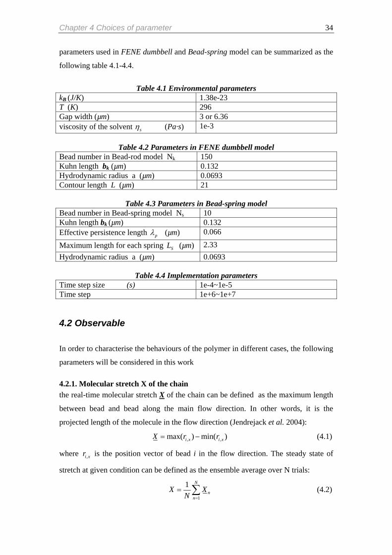
Chapter 4 Choices of parameter 34
parameters used in FENE dumbbell and Bead-spring model can be summarized as the
following table 4.1-4.4.
Table 4.1 Environmental parameters
kB (J/K) 1.38e-23 T (K) 296 Gap width (µm) 3 or 6.36 viscosity of the solvent sη (Pa·s) 1e-3
Table 4.2 Parameters in FENE dumbbell model
Bead number in Bead-rod model Nk 150 Kuhn length bk (µm) 0.132 Hydrodynamic radius a (µm) 0.0693 Contour length L (µm) 21
Table 4.3 Parameters in Bead-spring model Bead number in Bead-spring model Ns 10 Kuhn length bk (µm) 0.132 Effective persistence length pλ (µm) 0.066
Maximum length for each spring (µm) SL 2.33 Hydrodynamic radius a (µm) 0.0693
Table 4.4 Implementation parameters Time step size (s) 1e-4~1e-5 Time step 1e+6~1e+7
4.2 Observable
In order to characterise the behaviours of the polymer in different cases, the following
parameters will be considered in this work
4.2.1. Molecular stretch X of the chain the real-time molecular stretch X of the chain can be defined as the maximum length
between bead and bead along the main flow direction. In other words, it is the
projected length of the molecule in the flow direction (Jendrejack et al. 2004):
,max( ) min( )i x i x,X r= − r (4.1)
where is the position vector of bead i in the flow direction. The steady state of
stretch at given condition can be defined as the ensemble average over N trials:
,i xr
1
1 N
nn
X XN =
= ∑ (4.2)

Chapter 4 Choices of parameter 35
where n is the nth trial.
4.2.2. The longest relaxation time of molecular stretch
Figure 4.1 Relaxation curve of square of molecular stretch x2 of 21 um2 DNA by bead-spring model
The relaxation time of the molecular stretch is introduced to characterize the flow
strength. To obtain the longest relaxation time 1τ , we start the simulation from an initial
value of the stretch x/L =0.7 along the flow direction and run the simulation in absence
of flow and confined walls until the chains are completely relaxed. Averaging the
results over 40 repeat simulations, we can get a relaxation curve of square of molecular
stretch x2 as shown in Figure 4.1.The final 9 % of the curve can be fit into an
exponential curve as follows:
2
1
exp( )tx Aτ
B= − + (4.3)
where 1τ is the longest effective relaxation time, which is 0.11-0.13s for Bead-spring
(10 beads) model and 0.063 for FENE dumbbell model. This relaxation time is close
to the simulation result 0.095s by Jendrejack et al (2004). In addition, this relaxation
time indicates that the time step should not be larger than this value, therefore our
time step from 10-4-10-5 second sounds reasonable.
Chapter 4 Choices of parameter 36
4.2.3. The radius of gyration Rg of the chain The radius of gyration can be defined as follows:
2
1
1 bN
g iib
cR r rN =
= −∑ (4.4)
where rc is the center of mass of the chain as follows:
1
1 N
ciN =
= i∑r r (4.5)
where N is the number of beads and i is the index of the bead
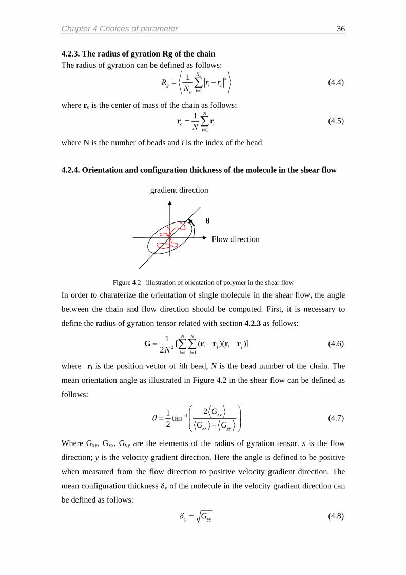
4.2.4. Orientation and configuration thickness of the molecule in the shear flow
Figure 4.2 illustration of orientation of polymer in the shear flow
In order to charaterize the orientation of single molecule in the shear flow, the angle
between the chain and flow direction should be computed. First, it is necessary to
define the radius of gyration tensor related with section 4.2.3 as follows:
21 1
1 [ ( )(2
N N
i j i ji jN = =
= −∑∑G r r r )]− r (4.6)
where ri is the position vector of ith bead, N is the bead number of the chain. The
mean orientation angle as illustrated in Figure 4.2 in the shear flow can be defined as
follows:
121 tan
2xy
xx yy
G
G Gθ −
⎛ ⎞⎜=⎜ −⎝ ⎠
⎟⎟
(4.7)
Where Gxy, Gxx, Gyy are the elements of the radius of gyration tensor. x is the flow
direction; y is the velocity gradient direction. Here the angle is defined to be positive
when measured from the flow direction to positive velocity gradient direction. The
mean configuration thickness δy of the molecule in the velocity gradient direction can
be defined as follows:
y yGδ = y (4.8)
Flow direction
gradient direction
θ

Chapter 4 Choices of parameter 37
4.2.5. Diffusivity coefficient of the chain In this case, polymer diffuses in the solution by Brownian kicks, the displacement of
center of mass in three directions can be given as the follows:
2 2 2 2x y z D= = = t (4.9)
then 2 6R Dt= (4.10)
Where D is the diffusion coefficient. Here is the plot of the <R2> vs t of 21 um DNA
by bead-spring model (10 beads) in the free solution without flow to check whether
the parameters are suitable.
10 100 1000
10
100
1000
<R(t)
2 > (u
m2 )
time (s)
D=0.28 um2/s
Figure 4.2 Mean-square displacement of center of mass vs, t for Bead-spring model (10)
As shown in Figure 4.2, the diffusion coefficient D of the chain is 0.286 µm2/s.
Compared with the input value 0.281 µm2/s we set in the simulation, Error= (0.286-
0.281)/0.281=0.18%, which indicates the validity of our method of obtaining the
coefficient from the simulations
4.2.6. steady state of center of mass distribution and width of center of mass distribution The steady state center of mass distribuation in the cross section of the channel can be
defined as follows:

Chapter 4 Choices of parameter 38
, ,( , ) ( ) ( )c c n NP y z y y z zδ δ= − − c n (4.11)
where yc,n and zc,n is the coordinates of center-of-mass in y and z direction at
observation n and N is the total number of trials for the simulation (Jendrejack et
al,2004).
In order to characterize to the depletion layer in the channel, the second moment of
the center-of-mass distribution in the cross section of the channel is introduced as
follows.
2 2 2( ) ( , )cw y z P y z dydz= +∫ (4.12)
The quantity w/weq gives a measure of the width of the center of mass distribution
relative to the equilibrium value (Jendrejack et al, 2004). If w/weq is increasing, it
indicates that the chain is migrating towards to the wall and vice verse.
Reference J.S.Hur, E.S.G.Shaqfeh, R.G.Larson, Brownian dynamics in simulations of single DNA molecules in
shear flow, J.Rheol.44, 713-742,2000
T.Perkins, D.E.Smith, R.G.Larson, S.Chu, Stretching of a single Tethered Polymer in a Uniform flow ,
Science, 268, 83-87,1995
R.G.Larson, The rheology of dilute solutions of flexible polymers: Progress and problems, J.Rheol.49,
1-70 , 2005
M.Chopra, R.G.Larson, Brownian dynamics simulations of isolated polymer molecules in shear flow
near adsorbin and nonadsorbing surface, J.Rheol.46,831- 862,2002
R.M.Jendrejack, D.C.Schwartz, J.J.de Pablo, M.D.Graham, Shear-induced migration in flowing polymer solutions: simulation of long-chain DNA in microchannels, J.Chem Phys,120,2513-2529,2004

Chapter 5 DNA in equilibriumTP PT 39
Chapter 5 DNA in equilibrium5
Before analyzing the sheared DNA in confined geometry, it is instructive to consider
the motion of single DNA molecule in equilibrium. With the variation of the length
scale of the geometry, the static properties of the chain are significant affected. This
can give us a simple picture about the dynamics of single DNA molecule in
equilibrium with confined boundaries.
5.1 Free solution in equilibrium
5.1.1. Analytical result In order to offer a comparison to the simulation, theoretical analysis is carried on first.
For simplicity, we take FENE dumbbell model to carry the theoretical analysis. Since
we have introduced the force law in the FENE dumbbell model as follows, we can get
the energy for each configuration Q, which is the end-to-end distance vector:
2
2max
1
HQ
Q
=−
QF (5.1)
2
2max2 20 0
max2max
1( ) ln(1 )21
Q Q
pHE d d HQ
Q QQ
= = = − −−
∫ ∫QQ F Q Q Q (5.2)
Where Qmax is the maximum molecular extension which means the contour length in
FENE dumbbell model and Ep is the potential energy for this configuration. Thus, the
configuration-space distribution function can be calculated based on the theory of
statistical physics as follows:
( , ) 1f d d =∫∫ Q P Q P (5.3)
( ) ( , )f dψ = ∫Q Q P P (5.4)
Where ( )ψ Q is the configuration-space distribution function and f(Q,P) is the phase-
space distribution function. To calculate this function, an important result from
5 Note: In this chapter, we didn’t consider hydrodynamic interaction if not specified
Chapter 5 DNA in equilibriumTP PT 40
classical statistical mechanics will be used: for a system at equilibrium, f(Q,P) is a
canonical distribution:
1( , ) exp( )f P H−= −Q Z B/k T
B
(5.5)
Where H is the Hamiltonian, the sum of the kinetic energy Ek and potential energy Ep
and Z is partition function, which can be given as follows:
max
0exp( H / ) exp( / ) exp( / )
Q
B k B pZ k T d d E k T d E k T d∞
∞
= − = − −∫ ∫ ∫ ∫+
-
Q P P Q (5.6)
By inserting Equation (5.2), it leads to:
2max
max2
220max
exp( / ) (1 ) B
HQQ k T
k BQZ E k T d d
Q
∞
∞
⎡ ⎤⎢ ⎥= − −⎢ ⎥⎣ ⎦
∫ ∫+
-
P Q (5.7)
By inserting Equation (5.5),Equation (5.4) can be rewritten as follows :
1
1
( ) exp( )
exp( / ) exp( / )p B k B
H T d
E k T E k T d
ψ −
+∞−
−∞
= −
= − −
∫
∫
Q Z P
Z P
B/k (5.8)
So the probability density of finding an end-to-end vector Q can be defined as
follows:
2 2max max
max2 2
2 2 22 20max max
( ) [1 ] (1 ) 4B B
HQ HQQk T k TQ Q Q dQ
Q Qψ π
⎡ ⎤⎢ ⎥= − −⎢ ⎥⎣ ⎦
∫Q (5.9)
This leads to the probability density of finding an end-to-end distance Q as follows:
2 2max max
max2 2
2 22 22 20max max
( ) 4 ( ) 4 [1 ] (1 ) 4B B
HQ HQQk T k TQ QP Q Q Q Q Q dQ
Q Qπ ψ π π
⎡ ⎤⎢ ⎥= = − −⎢ ⎥⎣ ⎦
∫ 2 (5.10)
Since we know the spring constant 2
3( 1)
B
K
k THN b
=−
, the constant in Eq (5.10) can be
rewritten as follows:
2max 3 ( 1
2 2 kB
HQ Nk T
)= − (5.11)
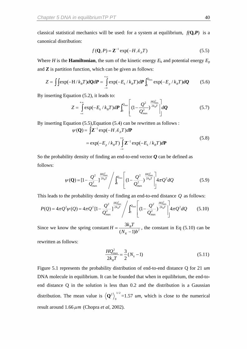
Figure 5.1 represents the probability distribution of end-to-end distance Q for 21 um
DNA molecule in equilibrium. It can be founded that when in equilibrium, the end-to-
end distance Q in the solution is less than 0.2 and the distribution is a Gaussian
distribution. The mean value is 1/ 22
0Q =1.57 um, which is close to the numerical
result around 1.66 mµ (Chopra et al, 2002).

Chapter 5 DNA in equilibriumTP PT 41
Figure 5.1 Probability distribution function of end-to-end distance for 21 um DNA molecule( Kuhn
step =150 ) by FENE dumbbell model, where the bin size is 0.001 and end-to-end distance normalized
by the maximum spring length Qmax
5.1.2 Simulation result In order to compare with the analytical results, DNA in free solution in equilibrium is
considered first. In this case, polymer molecule only experience the Brownian kicks
from surrounding solvent molecules, drag force which resists the movements, and
entropic spring forces which resist configurations changes of polymer molecules. For
this case, the molecular motion has been studied for 100s, and the length of time step
is chosen to 10-4-10-5 s. During this period, all the configuration data will be stored in
every 0.1 s around one relaxation time in order to collect the statistically significant
data for analysing the behaviour of the molecules with flow. In this way, we sampled
40-100 chains to get the ensemble properties of polymer, so the total number of
measure points is 40000-100000, which should be large enough to get good
approximation to real behaviour of polymers
FENE Dumbbell and Bead-spring model (10 beads) are implemented with their
corresponding force laws. By averaging those ensembles, statistical properties of
single chain in equilibrium can be shown in the following table.
Chapter 5 DNA in equilibriumTP PT 42
Table 5.1 Comparison of statistical properties by bead-spring and FENE model
Chorpra et al(2002) Bead-spring(10) FENE Equilibrium strech
1/ 22 /x L ( µm) 1.26(experimental) 1.13 0.74
End-to-end distance 1/ 22
0R ( µm) 1.66 1.43 1.48
Radius of gyration 1/ 22
GR ( µm) 0.68 0.64 0.74
1/ 220R /
1/ 22GR 2.44 2.23 2.00
As shown in Table 5.1, it can be seen that Bead-spring model have better agreements
with experimental value and simulation results in equilibrium in free solution from
Chorpra et al (2002) compared with FENE dumbbell model. However, it seems the
equilibrium stretch in the model doesn’t agree very well with the experimental value,
which indicates better parameters for bead-spring model can be found.
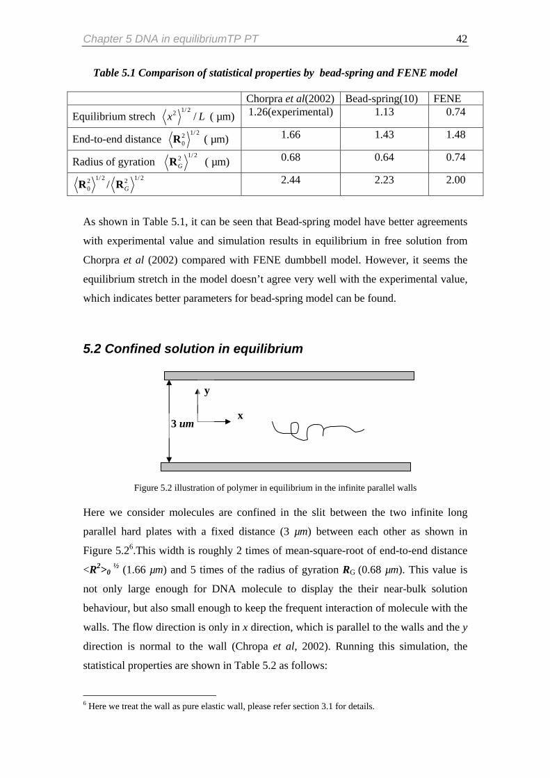
5.2 Confined solution in equilibrium
y
x3 um
Figure 5.2 illustration of polymer in equilibrium in the infinite parallel walls
Here we consider molecules are confined in the slit between the two infinite long
parallel hard plates with a fixed distance (3 µm) between each other as shown in
Figure 5.26.This width is roughly 2 times of mean-square-root of end-to-end distance
<R2>0 ½ (1.66 µm) and 5 times of the radius of gyration RG (0.68 µm). This value is
not only large enough for DNA molecule to display the their near-bulk solution
behaviour, but also small enough to keep the frequent interaction of molecule with the
walls. The flow direction is only in x direction, which is parallel to the walls and the y
direction is normal to the wall (Chropa et al, 2002). Running this simulation, the
statistical properties are shown in Table 5.2 as follows:
6 Here we treat the wall as pure elastic wall, please refer section 3.1 for details.
Chapter 5 DNA in equilibriumTP PT 43
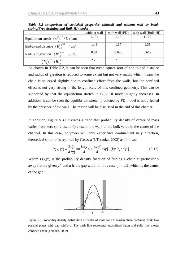
Table 5.2 comparison of statistical properties withwall and without wall by bead-spring(Free-draining and Bulk HI) model
without wall with wall (FD) with wall (Bulk HI)
Equilibrium strech 1/ 22 /x L ( µm) 1.121 1.12 1.129
End-to-end distance 1/ 22
0R ( µm) 1.43 1.37 1.35
Radius of gyration 1/ 22
GR ( µm) 0.64 0.626 0.619
1/ 220R /
1/ 22GR 2.23 2.19 2.18
As shown in Table 5.2, it can be seen that mean square root of end-to-end distance
and radius of gyration is reduced to some extent but not very much, which means the
chain is squeezed slightly due to confined effect from the walls, but the confined
effect is not very strong in the length scale of this confined geometry. This can be
supported by that the equilibrium stretch in Bulk HI model slightly increases. In
addition, it can be seen the equilibrium stretch predicted by FD model is not affected
by the presence of the wall. The reason will be discussed in the end of this chapter.
In addition, Figure 5.3 illustrates a trend that probability density of center of mass
varies from zero (or close to 0) close to the wall, to the bulk value in the center of the
channel. In this case, polymers will only experience confinement in y direction,
theoretical solution is reported by Casassa (I.Teraoka, 2002) as follows:
2
1
2 '( , ') sin sin exp[ ( / ) ]gk
k y k yP y y k R dd d d
π π π∞
=
= −∑ (5.12)
Where P(y,y’) is the probability density function of finding a chain at particular y
away from a given y’ and d is the gap width .In this case, y’ =d/2 ,which is the center
of the gap.
Figure 5.3 Probability density distribution of center of mass for a Gaussian chain confined inside two
parallel plates with gap width=d. The dash line represents unconfined chain and solid line means
confined chain (Teraoka, 2002)
Chapter 5 DNA in equilibriumTP PT 44
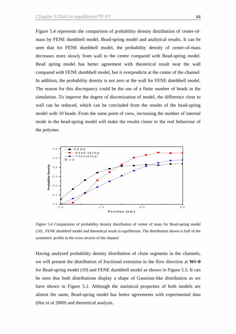
Figure 5.4 represents the comparison of probability density distribution of center-of-
mass by FENE dumbbell model, Bead-spring model and analytical results. It can be
seen that for FENE dumbbell model, the probability density of center-of-mass
decreases more slowly from wall to the centre compared with Bead-spring model.
Bead spring model has better agreement with theoretical result near the wall
compared with FENE dumbbell model, but it overpredicts at the center of the channel.
In addition, the probability density is not zero at the wall for FENE dumbbell model.
The reason for this discrepancy could be the use of a finite number of beads in the
simulation. To improve the degree of discretization of model, the difference close to
wall can be reduced, which can be concluded from the results of the bead-spring
model with 10 beads. From the same point of view, increasing the number of internal
mode in the bead-spring model will make the results closer to the real behaviour of
the polymer.
- 1 , 5 - 1 , 0 - 0 , 5 0 , 00 , 0
0 , 1
0 , 2
0 , 3
0 , 4
0 , 5
0 , 6
Prob
abili
ty D
ensi
ty
P o s i t io n ( u m )
F E N E B e a d - s p r in g T h e o r e t i c a l
W i = 0
Figure 5.4 Comparision of probability density distribution of center of mass for Bead-spring model
(10) , FENE dumbbell model and theoretical result in equilibrium. The distribution shown is half of the
symmetric profile in the cross section of the channel
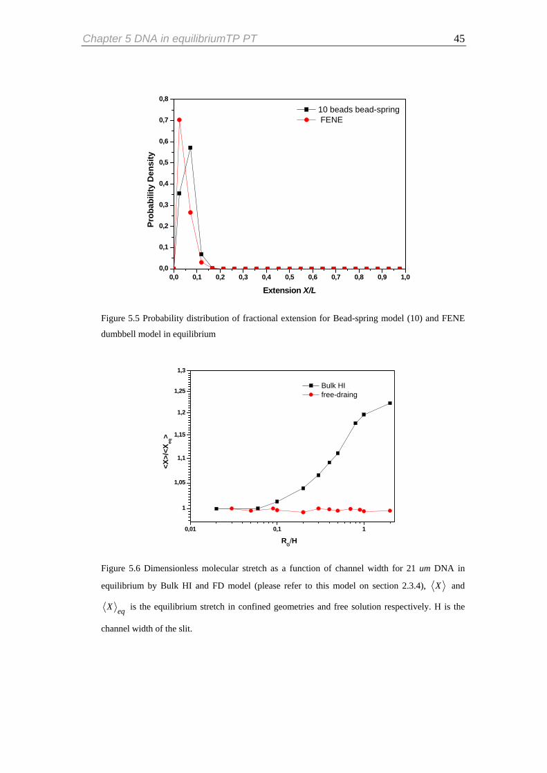
Having analysed probability density distribution of chain segments in the channels,
we will present the distribution of fractional extension in the flow direction at Wi=0
for Bead-spring model (10) and FENE dumbbell model as shown in Figure 5.5. It can
be seen that both distributions display a shape of Gaussian-like distribution as we
have shown in Figure 5.1. Although the statistical properties of both models are
almost the same, Bead-spring model has better agreements with experimental data
(Hur et al 2000) and theoretical analysis.
Chapter 5 DNA in equilibriumTP PT 45
0,0 0,1 0,2 0,3 0,4 0,5 0,6 0,7 0,8 0,9 1,00,0
0,1
0,2
0,3
0,4
0,5
0,6
0,7
0,8 10 beads bead-spring FENE
Prob
abili
ty D
ensi
ty
Extension X/L
Figure 5.5 Probability distribution of fractional extension for Bead-spring model (10) and FENE
dumbbell model in equilibrium
0,01 0,1 1
1
1,05
1,1
1,15
1,2
1,25
1,3
Bulk HI free-draing
<X>/
<Xeq
>
RG/H
Figure 5.6 Dimensionless molecular stretch as a function of channel width for 21 um DNA in
equilibrium by Bulk HI and FD model (please refer to this model on section 2.3.4), X and
eqX is the equilibrium stretch in confined geometries and free solution respectively. H is the
channel width of the slit.

Chapter 5 DNA in equilibriumTP PT 46
0,01 0,1 10,4
0,5
0,6
0,7
0,8
0,9
1
RG/H
D/D
free
Figure 5.7 Normalized diffusivity of the chain as a function of channel width for 21 um DNA in
equilibrium by Bulk HI model (please refer to this model on chapter 7), Dfree and D is the
diffusivity of the chain in free solution and confined geometry respectively. H is the channel width
of the slit. Figure 5.6 represents the equilibrium stretch of 21 um DNA molecule as a function of
the channel width in microchannels by free-draining model (without hydrodynamic
interaction and excluded volume interaction) and Bulk HI model7 (hydrodynamic
interaction). It can be seen that there is a transition region: the static confinement
effect appears at RG/H≈0.1, which means when H lowers down to around 10RG, the
chain will be strongly confined; Larger than this value, the confinement is not
pronounced. However, in the highly confined regime, for example when RG/H >2 is
not accurate, because the original bead-wall potential is not suitable for this model
anymore, since the bead-wall repulsive potential of the two walls in our model begins
to interfere with each other at this length scale. Compared to the chain in the channel
with a square cross section (Jendrejack et al, 2003), the stretch in the slit has a weaker
dependence on the channel width; there should be no plateau at the regime of smaller
channel width; the stretch should continue to increase as the decrease of the channel
width.
7 Please refer the concepts of Free-draining model and Bulk HI model in section 2.3.4 and section 7.2

Chapter 5 DNA in equilibriumTP PT 47
In addition, it can be seen that free-draining model can not predict the transition
regime of dimensionless molecular stretch from larger channel width to smaller
channel width and the stretch remains almost constant shown in Figure 5.6, it is quite
reasonable: Free-draining polymer chain in this parallel plates is equivalent to an ideal
chain in 3D random walk with confinement in y direction (wall-normal direction).The
stretch in other two unconfined directions x and z don’t change, since the random
walk in each direction is independent of each other.
In fact, Free-draining model with exclude volume interaction (but without
hydrodynamic interaction) also are examined. However, it gives the same prediction
with Free-draining model. At the first sight, this result is a little confusing. Because
according to theoretical prediction (de Gennes, 1979), the strong confinement will
also be expected at highly confined regime in a model with exclude volume
interaction. However, if you recall how we include this excluded volume interaction
in Equation (2.27) in chapter 2, it will be clear that we only consider the bonded
excluded volume interaction (the EV between a bead and its successive bead) and the
repulsive interactions between this bead and other surrounding beads are not explored,
since we switch off the bead-bead hydrodynamic interaction. This will lead to a
weaker EV effect even in extremely confined geometries.
It is related with Langevin equation Equation (2.27): it can be seen that all the non-
bonded interactions between bead and bead have to be incorporated through
hydrodynamic interaction. This also explains why we only see the confinement on
center of mass distribution, but almost no confined effect is predicted in molecular
stretch in the confined geometry for Free-draining model shown in table 5.2.
Besides the confinement on molecular stretch due to the confined geometry, the
diffusivity of the chain is also significantly affected by the confined boundary shown
in Figure 5.7. The simulations show that from around RG/H≈0.1, the diffusivity starts
to decrease significantly, which means highly confined effect will lead to a smaller
diffusion coefficient. This critical value for highly confined effect agrees with the
critical channel width in the molecular stretch. In addition, if we correlated with
simulation results in Figure 5.6 and 5.7, it can be noted that less stretched chains
move faster than highly stretched chains does. This is because the diffusivity of the
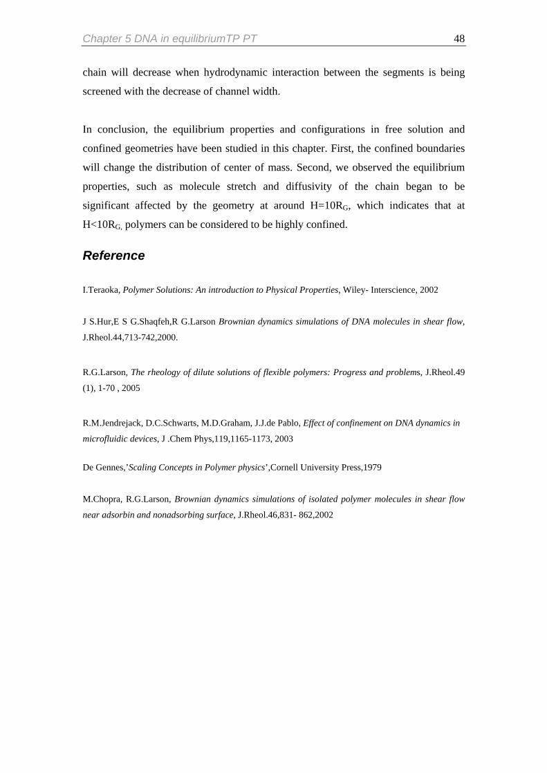
Chapter 5 DNA in equilibriumTP PT 48
chain will decrease when hydrodynamic interaction between the segments is being
screened with the decrease of channel width.
In conclusion, the equilibrium properties and configurations in free solution and
confined geometries have been studied in this chapter. First, the confined boundaries
will change the distribution of center of mass. Second, we observed the equilibrium
properties, such as molecule stretch and diffusivity of the chain began to be
significant affected by the geometry at around H=10RG, which indicates that at
H<10RG, polymers can be considered to be highly confined.
Reference I.Teraoka, Polymer Solutions: An introduction to Physical Properties, Wiley- Interscience, 2002
J S.Hur,E S G.Shaqfeh,R G.Larson Brownian dynamics simulations of DNA molecules in shear flow,
J.Rheol.44,713-742,2000.
R.G.Larson, The rheology of dilute solutions of flexible polymers: Progress and problems, J.Rheol.49
(1), 1-70 , 2005
R.M.Jendrejack, D.C.Schwarts, M.D.Graham, J.J.de Pablo, Effect of confinement on DNA dynamics in
microfluidic devices, J .Chem Phys,119,1165-1173, 2003
De Gennes,’Scaling Concepts in Polymer physics’,Cornell University Press,1979
M.Chopra, R.G.Larson, Brownian dynamics simulations of isolated polymer molecules in shear flow
near adsorbin and nonadsorbing surface, J.Rheol.46,831- 862,2002
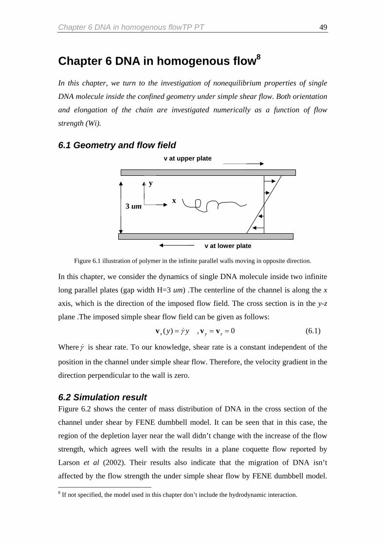
Chapter 6 DNA in homogenous flowTP PT 49
Chapter 6 DNA in homogenous flow8
In this chapter, we turn to the investigation of nonequilibrium properties of single
DNA molecule inside the confined geometry under simple shear flow. Both orientation
and elongation of the chain are investigated numerically as a function of flow
strength (Wi).
6.1 Geometry and flow field
Figure 6.1 illustration of polymer in the infinite parallel walls moving in opposite direction.
In this chapter, we consider the dynamics of single DNA molecule inside two infinite
long parallel plates (gap width H=3 um) .The centerline of the channel is along the x
axis, which is the direction of the imposed flow field. The cross section is in the y-z
plane .The imposed simple shear flow field can be given as follows:
( ) , 0x yy y zγ= = =v v& v (6.1)
Whereγ& is shear rate. To our knowledge, shear rate is a constant independent of the
position in the channel under simple shear flow. Therefore, the velocity gradient in the
direction perpendicular to the wall is zero.
6.2 Simulation result Figure 6.2 shows the center of mass distribution of DNA in the cross section of the
channel under shear by FENE dumbbell model. It can be seen that in this case, the
region of the depletion layer near the wall didn’t change with the increase of the flow
strength, which agrees well with the results in a plane coquette flow reported by
Larson et al (2002). Their results also indicate that the migration of DNA isn’t
affected by the flow strength the under simple shear flow by FENE dumbbell model. 8 If not specified, the model used in this chapter don’t include the hydrodynamic interaction.
y
x
v at upper plate
3 um
v at lower plate

Chapter 6 DNA in homogenous flowTP PT 50
The reason may be that the FENE dumbbell can not reproduce the complexity of the
configurational restrictions on the chain close to a confined boundary.
-1 ,5 -1 ,0 -0 ,5 0,00,0
0,1
0,2
0,3
0,4
0,5
0,6
0,7
Prob
abili
ty D
ensi
ty
P o sition (u m )
W i= 1 .3 W i= 6 .3 W i= 2 0 W i= 7 6
F E N E d u m b b e ll
Figure 6.2 Probability density distribution of center of mass for FENE dumbbell model with flow at
different Wi in the silt H=3 um
For Bead-spring model, it is similar with FENE dumbbell model. As shown in Figure
6.3, it can be seen the probability density distribution of the center-of -mass near the
wall didn’t change so much with the flow strength. However, Larson et al. (2002)
reported depletion layer near the wall should be decreased by the increase of the flow
strength. They hypothesized that the size of the chain will shrink in the shear gradient
direction at strong flow strength, which will allow the polymer to approach closer to
the wall. However, according to the results from the same group (Fang et al, 2005),
the opposite trends have been found. In addition, Pablo et al (1992) hold that the
thickness of depletion layer near the wall for Bead-rod model would decrease with the
increase of the flow strength from lower to intermediate flow strength, but increase
from intermediate flow strength to strong flow strength. They argued that at lower
shear rate, molecules would tend to align itself to the flow direction, thereby allowing
itself approach closer to the wall; at higher shear rate, molecule would rotate mole
rapidly, therefore it has more chances to interact with wall, which leads to the increase
of the thickness of the depletion layer of the wall. However, the region with
configuration restriction effect or steric effect from the wall is only around 1/3 to 1/2
of RG, so the presence of the wall only affects on the chain very close to the wall.
Therefore, with the increase of flow strength, the depletion region should not change

Chapter 6 DNA in homogenous flowTP PT 51
so much. Although weak migration behavior to the wall reported by Larson et al
(2002),it is still not consistent with the experimental results (Seo et al,1996).
-1 ,5 -1 ,0 -0 ,5 0 ,00 ,0
0 ,1
0 ,2
0 ,3
0 ,4
0 ,5
0 ,6
0 ,7
0 ,8
Prob
abili
ty D
ensi
ty
P o s it io n ( u m )
W e = 6 .3 W e = 7 6 W e = 1 2
B e a d - s p r in g
Figure 6.3 Probability density distribution of center of mass for 21um DNA by Bead-spring model with flow at different Wi in the silt H=3 um In order to test Larson’s idea, the mean orientation <θ> and the mean thickness δy of
DNA molecule in free solution and confined geometry at various flow strength are
examined in Figure 6.5. It can be seen that with the increase of the flow strength, the
mean orientation and the mean thickness δy will decrease, which indicates the chain
becomes slightly thinner in the velocity gradient direction and tends to align itself
closer to the flow direction. Those trends can be supported by the experimental results
at Wi <100 in free solution from Teixiara et al (2005) in Figure 6.4,
Figure 6.4 Probability distributions of (A) extension, (B) thickness, and (C) orientation. Both 22 um DNA (Wi =1.6 and 12) and 80 um DNA (Wi= 73) are shown. The bin sizes are 0.025, 0.05, and 1°, respectively (Teixiara et al ,2005)
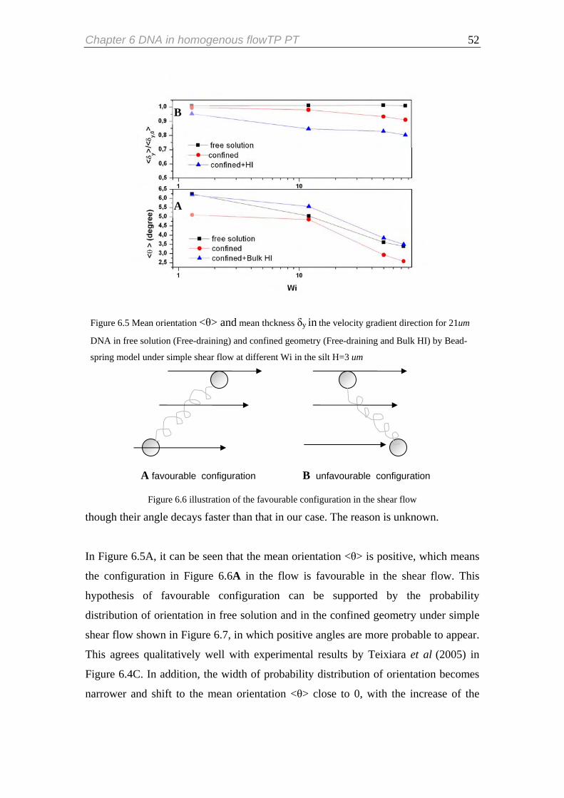
Chapter 6 DNA in homogenous flowTP PT 52
Figure 6.5 Mean orientation <θ> and mean thckness δy in the velocity gradient direction for 21um
DNA in free solution (Free-draining) and confined geometry (Free-draining and Bulk HI) by Bead-
spring model under simple shear flow at different Wi in the silt H=3 um
B
A
A favourable configuration B unfavourable configuration
Figure 6.6 illustration of the favourable configuration in the shear flow though their angle decays faster than that in our case. The reason is unknown.
In Figure 6.5A, it can be seen that the mean orientation <θ> is positive, which means
the configuration in Figure 6.6A in the flow is favourable in the shear flow. This
hypothesis of favourable configuration can be supported by the probability
distribution of orientation in free solution and in the confined geometry under simple
shear flow shown in Figure 6.7, in which positive angles are more probable to appear.
This agrees qualitatively well with experimental results by Teixiara et al (2005) in
Figure 6.4C. In addition, the width of probability distribution of orientation becomes
narrower and shift to the mean orientation <θ> close to 0, with the increase of the
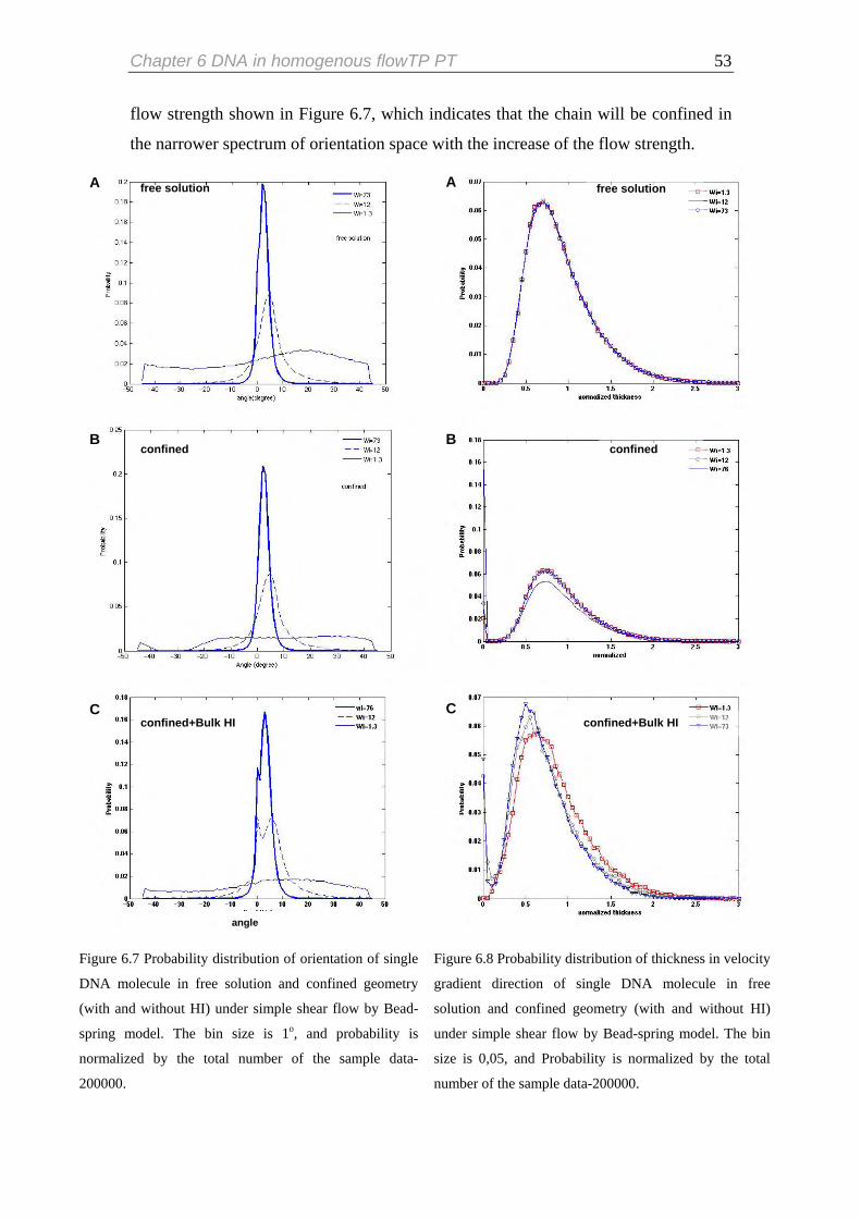
Chapter 6 DNA in homogenous flowTP PT 53
flow strength shown in Figure 6.7, which indicates that the chain will be confined in
the narrower spectrum of orientation space with the increase of the flow strength.
Figure 6.7 Probability distribution of orientation of single
DNA molecule in free solution and confined geometry
(with and without HI) under simple shear flow by Bead-
spring model. The bin size is 1o, and probability is
normalized by the total number of the sample data-
200000.
F
g
s
u
s
n
A free solution free solution
confined
confined+Bulk HI
angle
A
B
B confinedC
Cigure 6.8 Probability distribution of thickness in velocity
radient direction of single DNA molecule in free
olution and confined geometry (with and without HI)
nder simple shear flow by Bead-spring model. The bin
ize is 0,05, and Probability is normalized by the total
umber of the sample data-200000.
confined+Bulk HI

Chapter 6 DNA in homogenous flowTP PT 54
However, we didn’t find that the mean thickness δy of single molecule in gradient
direction change so much but almost remain constant as shown in Figure 6.5B for the
case free solution and confined geometry by Free-draining model, even the
probability distribution of the thickness almost remain unaffected by the flow strength
shown in Figure 6.8A,B. However, when hydrodynamic interaction (Bulk HI) comes
into the play, things become different. The mean thickness δy decay a lot with the
increase of flow strength compared with other two models shown in Figure 6.5B,
which can be supported by that the thickness distribution shifts to small thickness
direction with increase of the flow strength shown in Figure 6.8C. The result about δy
predicted by considering the hydrodynamic interaction is similar with the
experimental result in Figure 6.4B, which indicates hydrodynamic interaction can
strongly induce the decrease of the mean thickness δy
Furthermore, as shown in Figure 6.7-6.8, only the model with hydrodynamic
interaction (Bulk HI) gives correct predictions on all the dynamic properties compared
with the experimental results in Figure 6.4, though other two models (Free solution
and confined solution by Free draining model) gives partial correct predictions,
which hydrodynamic interaction plays an important role on the variation of the shape
of molecule in the solution under shear flow but less important on other properties,
such as the distribution of orientation.
0 5 10 15 200,0
0,1
0,2
0,3
0,4
0,5
0,6
0,7
Prob
abili
ty D
ensi
ty
molecular stretch X (um)
Wi=6.3Wi=1.3Wi=76
FENE
Figure 6.9 Probability distribution of fractional extension for 21um DNA by FENE dumbbell model
with flow at different Wi
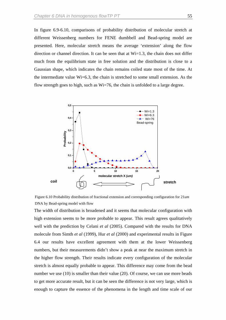
Chapter 6 DNA in homogenous flowTP PT 55
In figure 6.9-6.10, comparisons of probability distribution of molecular stretch at
different Weissenberg numbers for FENE dumbbell and Bead-spring model are
presented. Here, molecular stretch means the average ‘extension’ along the flow
direction or channel direction. It can be seen that at Wi=1.3, the chain does not differ
much from the equilibrium state in free solution and the distribution is close to a
Gaussian shape, which indicates the chain remains coiled state most of the time. At
the intermediate value Wi=6.3, the chain is stretched to some small extension. As the
flow strength goes to high, such as Wi=76, the chain is unfolded to a large degree.
0 5 10 15 200,0
0,1
0,2
0,3
0,4
0,5
Prob
abili
ty
molecular stretch X (um)
Wi=1.3 Wi=6.3 Wi=76
Bead-spring
Figure 6.10 Probability distribution of fractional extension and corresponding configuration for 21um
DNA by Bead-spring model with flow
stretch coil
The width of distribution is broadened and it seems that molecular configuration with
high extension seems to be more probable to appear. This result agrees qualitatively
well with the prediction by Celani et al (2005). Compared with the results for DNA
molecule from Simth et al (1999), Hur et al (2000) and experimental results in Figure
6.4 our results have excellent agreement with them at the lower Weissenberg
numbers, but their measurements didn’t show a peak at near the maximum stretch in
the higher flow strength. Their results indicate every configuration of the molecular
stretch is almost equally probable to appear. This difference may come from the bead
number we use (10) is smaller than their value (20). Of course, we can use more beads
to get more accurate result, but it can be seen the difference is not very large, which is
enough to capture the essence of the phenomena in the length and time scale of our

Chapter 6 DNA in homogenous flowTP PT 56
confined geometry shown in Figure 6.1. In addition, as the increase of flow strength,
the fractional molecular stretch asymptotes to around 0.5 shown in Figure 6.11 ,
which is similar with the value of 0.5 from Hur et al (2000). This is interesting: it
means the average molecular stretch will remain 0.5 even at very high shear rate.
Larson (2005) explained these phenomena according to the observation by Simth et al
(1999): The chain tends to align itself to the flow direction under flow strength.
However, Brownian force will kick the beads out of the shear plane with a positive or
negative angle shown in Figure 6.13. According to our knowledge on fluid dynamics,
a simple shear flow can be regarded as the superimposition of pure elongation flow
and pure rotation flow shown in Figure 6.12. Due to the coupling of those two flow
effects, the dynamics of polymer molecules in the shear flow will become
complicated. After being kicked out of the shear plane, there will be two possibilities
for a stretched chain: for the positive angle, drag force will stretch molecular further
and the vorticity will derive the molecular back to the shear plane; for negative angle,
drag force will help the chain relax and vorticity will carry it to the shear plane shown
in Figure 6.13. After coming back, the molecule will be kicked out of the shear plane
and then repeat the above process. During this process, DNA molecule will
experience stretching, tumbling, coiling state irregularly. Based on this mechanism,
although molecule has more chances to stretch, it also has a substantial probability to
tumble, so the average stretch approaches to 0.5 even at the higher shear rate (Larson,
2005)
0 20 40 60 80 100 1200.0
0.1
0.2
0.3
0.4
0.5
0.6
0.7
0.8
0.9
1.0
Frac
tiona
l str
etch
Wi
Bead-spring
Figure 6.11 average fractional extension of 21um DNA by Bead-spring model at different Wi

Chapter 6 DNA in homogenous flowTP PT 57
Figure 6.12 illustration of simple shear flow can be regarded as the superposition of the pure elongation
flow and pure rotation flow
rotation shear elongation
stretch tumble
positive angle negative angle
Figure 6.13 illustration of the tumbling dynamics of polymer in the simple shear flow In this chapter, dynamics of DNA molecule under simple shear flow in the confined
geometry is investigated. It can be seen that statistical properties of single DNA
molecule, such as probability density distribution of center of mass in physical space,
have been significantly affected. As the increase of flow strength, the chain will be
confined in a narrower orientation space and hydrodynamic interaction becomes
important when we consider the variation of the size of molecule in the velocity
gradient direction. This indicates that hydrodynamic interaction will play an import
role on some nonequilibrium properties, and we will discuss this effect in detail in
chapter 7.
So far, migration behavior of DNA molecule due to the variation of the flow strength
is not discovered in those models without including hydrodynamic interaction, which
doesn’t agree with experimental results (Ausserre et al, 1991, Seo et al, 1996) and
simulation results from others (Hur et al 2000, Pablo et al 1992). There are several
reasons for these discrepancy mentioned by Pablo et al (1992): first, we neglect the
hydrodynamic interaction between bead and bead. Second, hydrodynamic interaction
created by the confined geometry has been neglected for simplicity. Third, since
molecules have less probability to appear to the region near the wall, it should create

Chapter 6 DNA in homogenous flowTP PT 58
inhomogeneous flow, but we assume the flow field won’t be disturbed. Those
simplifications should be questioned; we will incorporate those effects into the next
chapter.
Reference
M.Chopra, R.G.Larson, Brownian dynamics simulations of isolated polymer molecules in shear flow
near adsorbin and nonadsorbing surface, J.Rheol.46,831- 862,2002
J.J.de Pablo, H.C.Ottiinger , Hydrodynamic Changes of the Depletion Layer of Dilute Polymer
Solutions Near a wall ,AlchE Journal,308,1992
Ausserre, D., J.Edwards, J.Lecourtier, H.Hervet, F.Rondelez, Hydrodynamic thickening of the
depletion layer in colloidal solutions, Europhys,Lett,14,33-38,1991
Y.H.Seo, O.O.Park, M.S.Chun, The behavior of the velocity enhancement in microcapillary flows of
flexible water-soluable polymers,J.Chem.Eng.Jpn,29,611,1996
R.E. Teixeira, H P. Babcock,E.S. G. Shaqfeh, S.Chu, Shear Thinning and Tumbling Dynamics of
Single Polymers in the Flow-Gradient Plane , Macromolecules 38, 581-592,2005
Simth,D.E, H.P.Babcock, S.Chu, Single polymer dynamics in steady shear flow, Science 283,1724-
1727,1999
J S.Hur,E S G.Shaqfeh,R G.Larson Brownian dynamics simulations of DNA molecules in shear flow,
J.Rheol.44,713-742,2000.
R.G.Larson, The rheology of dilute solutions of flexible polymers: Progress and problems, J.Rheol.49
(1), 1-70, 2005
L.F, H.Hu, R.G.Larson, DNA configurations and concentration in shearing flow near a glass surface in a microchannel, J. Rheol.49,127-138,2005
A. Celani, A.Puliafito, K.Turitsyn, Polymers in linear shear flow: a numerical study, Europhys. Lett.,
70 , 464-470, 2005

Chapter 7 DNA in inhomogeneous flow 59
Chapter 7 DNA in inhomogeneous flow
In the last chapter, Dynamics of single DNA molecule in the confined geometry under
the homogenous flow (simple shear flow) has been investigated. It can be seen that
DNA molecules display different behaviors in confined geometry compared to the
case in the free solution. But we didn’t find the migration effect near the wall as
people reported migration toward the wall (Pablo et al 1992, Larson et al. 2002) or
migration to the center of the channel (Seo et al 1996, Jendrejack et al, 2004). As
mentioned before, that’s because we did some assumptions for simplicity. In this
chapter, those neglected effects in our model will be taken into the play, especially the
influence of the wall to the hydrodynamic flow.
7.1 Geometry and flow field
Figure 7.1 illustration of single DNA molecule in a microchannel with a square cross section and
velocity profile under pressure-driven flow. x is the flow direction
In this chapter, we considered the dynamics of single DNA molecule in an infinite
long microchannel with a square cross section (gap width H=6.36 um) .The center line
of the channel is along the x axis, which is the direction of the imposed flow field.
Thus, the cross section is in the y-z plane .The imposed pressure-driven flow field can
be given by Jendrejack et al (2004) as follows:
2
( 1) / 23 3
1,3,5
4 cosh( / ) cos( / )( , ) ( ) ( 1) [1 ]cosh( / 2)
kx
k
H dp k z H k y Hy zdx k k
π πηπ π
∞−
=
= − − × −∑vK
(7.1)
x ( flow direction )
y
x
P(0)=P0+∆P P(L)=P0
y
z
H
L
L=63.6um
H=6.36um

Chapter 7 DNA in inhomogeneous flow 60
Where -dp/dx is the pressure difference along the flow direction, η is the viscosity of
the solution, H is the width of the channel. The strength of the flow is defined by an
effective shear rate, max2 /eff v Hγ =& , where max (( 0, 0))y z= = =v v is the velocity at
the center line of the channel.
7.2 Hydrodynamic Interaction model In this chapter, three models with different levels to treat hydrodynamic interaction
are compared9. The hydrodynamic interaction can be incorporated into Brownian
dynamics through hydrodynamic interaction tensor in the diffusion tensor
shown in Equation (2.27) and (2.30) as follows:
ijΩ ijD
1/ 2
1 1 1
6N N Nij si
i ij ij j jj B
ddt k T dt= = =
∂ ⎛ ⎞= ⋅ + ⋅ + + ⋅⎜ ⎟∂ ⎝ ⎠∑ ∑ ∑
Dr κ r D F Br ij in
1( )6ij B ij ij
s
k Ta
δπη
= +D I Ω
The simplest model to treat the hydrodynamic interaction is Free-Draining model,
which means the hydrodynamic interaction is neglected and a bead will not be
affected by the flow field due to the motion of its surrounding beads. Therefore, the
diffusion tensor can be expressed as follows:
ijΩ
6
FD Bij ij
k Taδ
πη=D I (7.2)
Here it can be seen that is a symmetric, isotropic and position-independent
tensor.
FDijD
A more accurate approximation to describe the hydrodynamic interaction is Bulk
Hydrodynamic Interaction model. Hydrodynamic interaction between bead and bead
in free solution is included into the diffusion tensor as follows:
1 (1 )6
Bulk RPYij B ij ij ijk T
aδ δ
πη⎡ ⎤
= + −⎢ ⎥⎣ ⎦
D I Ω (7.3)
Where is the Rotne-Prager-Yamakawa (RPY) Tensor mentioned in chapter 2.
It is a symmetric, but anisotropic and inter-configuration dependent tensor, which
leads to configuration-dependent and anisotropic diffusion tensor.
RPYijΩ
9 These three models we have metioned in Chapter 2
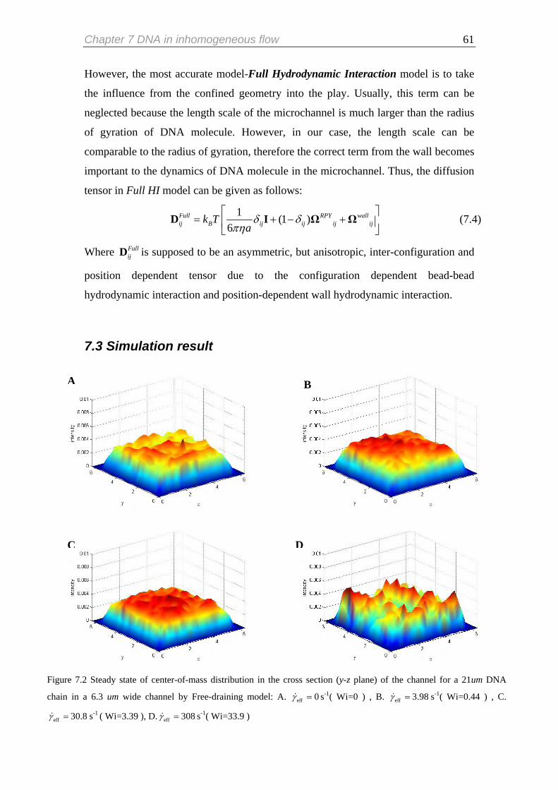
Chapter 7 DNA in inhomogeneous flow 61
However, the most accurate model-Full Hydrodynamic Interaction model is to take
the influence from the confined geometry into the play. Usually, this term can be
neglected because the length scale of the microchannel is much larger than the radius
of gyration of DNA molecule. However, in our case, the length scale can be
comparable to the radius of gyration, therefore the correct term from the wall becomes
important to the dynamics of DNA molecule in the microchannel. Thus, the diffusion
tensor in Full HI model can be given as follows:
1 (1 )6
Full RPY wallij B ij ij ij ijk T
aδ δ
πη⎡
= + − +⎢⎣ ⎦
D I Ω Ω ⎤⎥ (7.4)
Where is supposed to be an asymmetric, but anisotropic, inter-configuration and
position dependent tensor due to the configuration dependent bead-bead
hydrodynamic interaction and position-dependent wall hydrodynamic interaction.
FullijD
7.3 Simulation result
Figu
chai
effγ&
B
AC
re 7.2 Steady state of center-of-mass distribution in the cr
n in a 6.3 um wide channel by Free-draining model: A.
30.8= s-1 ( Wi=3.39 ), D. eff 308γ =& s-1( Wi=33.9 )
D
oss section (y-z plane) of the channel for a 21um DNA
eff 0γ =& s-1( Wi=0 ) , B. eff 3.98γ =& s-1( Wi=0.44 ) , C.

Chapter 7 DNA in inhomogeneous flow 62
The effect of the flow strength on the probability distribution of center-of-mass is
represented in Figure 7.2 for a 21 um DNA molecule by Free-draining model. At
equilibrium (Wi=0), the center-of-mass has a uniform distribution across the channel,
except a depletion layer near the wall (Blue area) due to steric hindrance from the
wall. As the increase of the flow strength, the depletion layer near the wall is
unaffected, which can be quantified by the width of the center-of-mass in the Figure
7.8.This is similar with the phenomena we observed in the simple shear flow in
chapter 6 (the reason will be discussed later). However, this is not consistent with the
experimental results by Fang et al (2004), they reported that the depletion layer will
be enlarged with the increase of the flow strength.
Figu
chan
effγ&
nosi
obse
B
Are 7.3 Steady state of stretch as a function of position of c
nel for a 21um DNA chain in a 6.3 um wide channel by
3.98= s-1( Wi=0.44 ) , C. eff 30.8γ =& s-1 ( Wi=3.39 ), D. effγ&
y due to the small observations near the wall(the error is prop
rvations.)
C
e
o
D
nter-of-mass in the cross section (y-z plane) of the
Free-draining model : A. eff 0γ =& s-1( Wi=0 ) , B.
308= s-1( Wi=3.39 ).The data around the edges are
rtional to N-1/2 where N is the number of independent

Chapter 7 DNA in inhomogeneous flow 63
Figure 7.3 represents the influence of flow strength on the probability distribution of
chain stretch in the cross section of the channel for a 21 um DNA molecule by Free-
draining model. These plots are plotted as the average stretch at given position in the
cross section in order to decouple it from the probability of finding a chain at this
position. It can be seen that the distribution is uniform at equilibrium (the blue area
means the small probability of finding a chain there), the chain in the depletion layer
is slightly more elongated than that in the center of the channel due to the steric
hinderance. It’s because only higher stretched chain parallel to wall can survive in the
region near the wall as illustrated in Figure 7.4. Because less restricted configuration
has a larger thickness in the direction perpendicular to the wall, so at the same
distance above the wall, the chain with this configuration can be pushed away from
the wall first. Therefore, it leads to a lower density of center-of-mass near the wall but
higher average strength there.
Figure 7.4 illustration of configurations of the chain near the lower wall. The red area is the region
where the chain can feel the repulsive force from the lower wall.
As the increase of the flow strength, the chain is highly elongated if we compared the
4 plots in the Figure 7.3. The probability distribution of the chain extension becomes
highly nonuniform compared with the equilibrium case. At higher Weissenberg
number, the chain near the wall are strongly aligned and elongated to the flow
direction against the randomizing influence of Brownian motion, but the chain near
the center is less elongated at the center line of the channel, and a minimum of the
averaged stretch is shown in Figure 7.3 B, C, D. This is due to the inhomogeneous
properties of the parabolic flow, the local velocity gradient near the wall is higher than
that near the center of the channel, which means the shear rate near the wall is higher
than that near the center.
In Figure 7.5 A, B, C, the effect of the flow strength on the probability distribution of
center-of-mass is represented for a 21 um DNA molecule by Bulk HI model.
more elongated less restricted F F=
exclued region
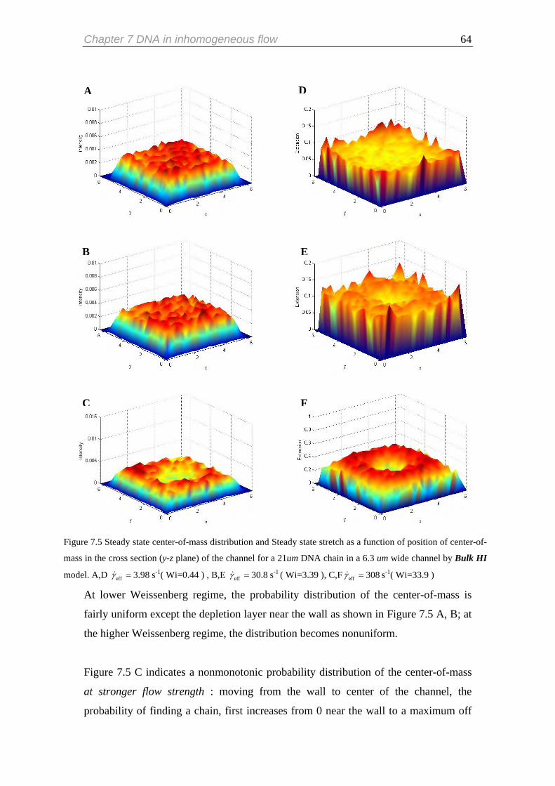
Chapter 7 DNA in inhomogeneous flow 64
Figu
mas
mod
A
B E
FC
re 7.5 Steady state center-of-mass distribution and Stead
s in the cross section (y-z plane) of the channel for a 21um
el. A,D eff 3.98γ =& s-1( Wi=0.44 ) , B,E eff 30.8γ =& s-1 ( W
At lower Weissenberg regime, the probabilit
fairly uniform except the depletion layer near t
the higher Weissenberg regime, the distribution
Figure 7.5 C indicates a nonmonotonic probab
at stronger flow strength : moving from th
probability of finding a chain, first increases f
D
y
y
state stretch as a function of position of center-of-
DNA chain in a 6.3 um wide channel by Bulk HI
i=3.39 ), C,F eff 308γ =& s-1( Wi=33.9 )
distribution of the center-of-mass is
he wall as shown in Figure 7.5 A, B; at
becomes nonuniform.
ility distribution of the center-of-mass
e wall to center of the channel, the
rom 0 near the wall to a maximum off

Chapter 7 DNA in inhomogeneous flow 65
the centerline (near the wall), then decrease to a local minimum at the centerline. The
maximum is the consequence of the competition between the steric hinderance from
the wall and the spatial variation of the bead-bead hydrodynamic interation produced
by the inhomogeneous flow. The steric effect will give the repulsive force to drive the
molecule (very close to the wall) away from the wall, but the spatial variation of the
diffusivity along the chain in the velocity gradient direction will make the chain
migrate out of regions of lower shear rate to regions of higher shear rate. Therefore, a
maximum appears near the wall, which can be illustrated as a simple picture in Figure
7.6. As known from Chapter 6, the chain has fewer configurations in gradient
direction and orientates almost parallel to the flow direction at strong shear rate; at
smaller shear rate, the chain has more configurations in gradient direction. Therefore,
the simple mechanism is: the chain near the center (lower shear rate) migrates
towards wall due to an implicitly position-dependent diffusivity (induced by the
configuration-dependent hydrodynamic interaction). When it enters into the excluded
region near the wall, the contribution to the drift toward wall from the diffusion
becomes less important; at the same time, the drift term toward the center contributed
by the repulsive wall becomes important. At a particular point near the wall, the
upward drift term will be equal or larger than the downward drift term. This is where
the maximum is.
Figure 7.6 illustration of the mechanism of migration behavior of the chain in the microchannel
predicted by Bulk HI model. The area below the dash line is the region where the chain can feel the
repulsive force from the lower wall. Here we only plot the lower wall for simplicity. x and y is flow
direction and its velocity gradient direction.
In addition, it can be seen in Figure 7.8 that as the increase of the flow strength, the
width of center-of-mass is slightly increased, which indicates the chain migrates
toward the wall and leads to a thinner depletion layer. It is because the flow strength
fewer configurations, almost parallel to the wall
more configurations, variation of the diffusivity along the chain
Vup
y x
Vdown
excluded region

Chapter 7 DNA in inhomogeneous flow 66
increases, the velocity gradient perpendicular to the wall is increased compared to the
smaller flow strength, which indicates the variation of diffusivity along the chain(near
the center) is larger at stronger flow strength. This stronger driving force under the
stronger flow strength makes the chain migrate towards the wall further compared
with the case in smaller flow strength.
Figure 7.5 D, E, F show the average stretch in the cross section is increased with the
increase of the flow strength and the distribution is still nonuniform as we observed in
the Free-draining model. At lower Weissenberg number, the average stretch
decreases monotonically from the maximum near the wall to the minimum in the
center. The reason is the same: higher local velocity gradient induced the higher
extension near the wall. The only difference is that the average stretch in the local
minimum is not as low as that predicted by Free-draining model if we compared with
Figure 7.3C and Figure 7.5 E. The reason is unknown. It may be because part of the
less stretched chains migrate toward wall and highly elongated chains will migrate
toward the center, so the probability of finding a less stretched chain becomes smaller
near the center, therefore the chain in the center of the channel is predicted with
higher average stretch in Bulk HI model compared with that predicted by Free-
draining model. In other words, because of the migration of less stretched chain, you
can find a less extended chain in the region near the wall with a relatively higher
probability, and more higher stretch molecules near the center, which means the
average stretch in the region near the center is higher and a relatively smaller stretch is
predicted near the wall compared with that in Figure 7.3
So far, it seems that we got a reasonable result for the migration behavior, but this is
not the case, which has an opposite trend on migration behavior. It is because we
didn’t treat the contribution to the flow field from the wall in an accurate way.
Although the steric effect has been considered, it is only restricted itself in a boundary
layer near the wall, which is a short-range interaction and will not influence the whole
velocity field. Therefore, it is necessary to include the wall hydrodynamic interaction,
which is Full HI model, to see any difference there.

Chapter 7 DNA in inhomogeneous flow 67
02
46
0
2
4
60
0.02
0.04
0.06
0.08
0.1
xy
inte
nsity
Figure 7.7 Steady state center-of-mass distribution and Steady state of stretch as a function of position of center-
of-mass in the cross section (y-z plane) of the channel for a 21um DNA chain in a 6.3 um wide channel by Full
HI model. A,D eff 3.98γ =& s-1( Wi=0.44 ) , B,E eff 30.8γ =& s-1 ( Wi=3.39 ), C,F eff 308γ =& s-1( Wi=33.9 )
DA
EB
FC
Figures 7.7 A, B, C illustrate the effect of flow strength on the probability distribution
of the center-of-mass distribution. It can be seen that as the increase of the flow
strength, a hydrodynamic-induced depletion layer (red area) is forming and depletion
effect is quite strong at stronger flow strength. This can be supported by Figure7.8:
the width of center-of-mass distribution in the cross section of the channel is
decreasing with the increase of the flow strength, which indicates the depletion layer

Chapter 7 DNA in inhomogeneous flow 68
is enlarging. Figure 7.7 C also indicates the distribution increases nonmonotonically
from the pronounced depletion area near the wall and peaks at the halfway between
the wall and the center, and then decreases to the local minimum in the center. This is
due to the Brownian drift away from the centerline and deterministic drift away from
the wall (due to the asymmetry of the bead mobility and wall hydrodynamic
interaction due to the presence of the wall). The details of the mechanism will be
discussed in the next section.
Figure 7.7 D,E,F show the average stretch in the cross section is increased with the
increase of the flow strength. At the lower Weissenberg number, the distribution is
fairly uniform, except the depletion layer near wall; higher strength appears there
which is similar with those we have observed in the previous two models. At stronger
flow strength, the maximum of average stretch seems to peak at halfway between the
center and wall. This maybe because the less stretched chain will migrate toward the
wall, while highly elongated chain near the wall drift away from the wall due to the
presence of the wall. Therefore, the competition of those two effects leads to
nonmontonical distribution of molecular stretch in the cross-section of the channel.
0 5 10 15 20 25 30 35
0,995
1,000
1,005
1,010
1,015
1,020
w/w
eq
Wi
FD Bulk HI Full HI
Figure 7.8 Width of the steady-state center-of-mass distribution w (relative to equilibrium weq) in the
microchannel as a function of flow strength for 21 um DNA by Free-draining model (black),Bulk HI
model (red),and Full HI model (blue).
Chapter 7 DNA in inhomogeneous flow 69
Figure 7.8 represents the width of the steady-state center-of-mass distribution
normalized by the equilibrium width as a function of flow strength. Results are shown
for Free-draining model, Bulk HI model, and Full HI model. It can be seen that the
width is unaffected with the variation of the flow strength in Free-draining model,
which means migration effect is not expected by this model. For Bulk HI model, the
width slightly increases with the flow strength, which indicates weak migration
toward the wall. In addition to Full HI model, the width decrease a lot compared with
other two models, therefore migration away from the wall is predicted and the
depletion layer increases with the flow strength. Those results indicate that molecular
migration away from the wall is induced by the coupling of bead-bead hydrodynamic
interaction and hydrodynamic effect from the confined geometry.The mechanism in
details will be discussed in the next section.
7.4 Mechanism on migration behavior
7.4.1. General analytical approach In the last section, the different migration behaviors under pressure-driven flow in the
confined geometry have been predicted by different hydrodynamic interaction model.
So far, only Full HI model gives a correct prediction to migration behavior. The
depletion layer is significant affected by the variation of the flow strength, which
indicates the chain migrates toward the center of the microchannel. Various
mechanisms have been explored in order to explain the migration behavior in
confined geometries. From Jendrejack et al’s work (2004), it is now well accepted
that configuration dependent hydrodynamic interaction coupled with inhomogenous
shear flow and confined boundaries are most likely responsible for the migration
across streamlines. In this section, Jendrejack’s idea is followed and simple modified
mechanism will be proposed.
To explain those phenomena, the theoretical analysis of elastic dumbbell model (two
beads connected by a spring) is carried through the generalized diffusion equation.
The probability distribution functionΨ for a single dumbbell is a function of positions
of two beads (r1, r2) and time (t) in physical space. So the continuity equation for
(rΨ 1, r2,t) can be given as follows (Bird et al, 1987):
1 21 2
( ) (t
)∂Ψ ∂ ∂= − ⋅ Ψ − ⋅ Ψ
∂ ∂ ∂r r
r r& & (7.5)
Chapter 7 DNA in inhomogeneous flow 70
where , is the velocity of beads at the r1r& 2r& 1, r2. Since the relationship between r1, r2 and center of mass rc and the connector vector q as follows: 1 22 (c )= +r r r (7.6)
2 1= −q r r (7.7)
112c= −r r q (7.8)
212c= +r r q (7.9)
So the following derivatives can be got:
1 2
1 2 1c c c
∂ ∂∂ ∂ ∂ ∂ ∂= + = +
∂ ∂ ∂ ∂ ∂ ∂ ∂q q
r rr r r r r r r2
(7.10)
1 2
1 2 2
1 (2
c c
∂ ∂∂ ∂ ∂ ∂ ∂= + = −
∂ ∂ ∂ ∂ ∂ ∂ ∂r r
r rq r q r q r r1
) (7.11)
Subsituting (7.6)-(7.11) into (7.5), Equation (7.5) can be rewritten as follows:
1 21 2
1
( ) ( )
1 1( ) ( )2 2
( ) ( )
c c
cc
t∂Ψ ∂ ∂
= − ⋅ Ψ − ⋅ Ψ∂ ∂ ∂
∂ ∂ ∂ ∂= − − ⋅ Ψ − + ⋅ Ψ
∂ ∂ ∂ ∂∂ ∂
= − ⋅ Ψ − ⋅ Ψ∂ ∂
r rr r
rr q r q
r qr q
& &
&
& &
2r& (7.12)
Where the average velocity of center of mass rc is given as follows (Bird et al 1977)
2 2
1 2, 1 , 1
2 ( ) lnsj
c ij iji j i jB jk T= =
∂= ⋅ + + ⋅ − ⋅ Ψ
∂∑ ∑F
r κ r r D Dr
& (7.13)
and average time evolution rate of connector vector q is : &
2 2
2 1 2 1 2 11 1
( ) ( ) ( ) lsj
j j j jj jB jk T= =
∂= ⋅ − + − ⋅ − − ⋅ Ψ
∂∑ ∑F
q κ r r D D D Dr
& n (7.14)
Now it can be seen that the probability distribution functionΨ can be rewritten as a
function of center of mass r( , , )c tΨ r q c and the connector vector q. But what we are
really interested in the relationship between Ψ and position center of mass rc. Therefore,
we integrate Equation (7.12) in order to decouple the influence of q and rc :
( , ) ( , , )c cC t t d= Ψ∫r r q q (7.15)
So the continuity equation for center of mass rc can be given as follows:
( , )c
cc
C tt
∂= −∇ ⋅
∂ rr j (7.16)

Chapter 7 DNA in inhomogeneous flow 71
where is the probability distribution of center of mass r( , )cC tr c and c c C=j r& is the
momentum-space-averaged center-of-mass, integrated over the internal degrees of
freedom of the chain, and the average is defined as follow:
A A d= Ψ∫ q (7.17)
Therefore c Cr& can be got by multiplying Equation (7.13) by Ψ and integrate by
connector vector q :
First, we rewrite the r as follows rc:
1 1 1ˆ( ln ln2 4 2
sc c
c)∂ ∂
= + ⋅ − Ψ − Ψ∂ ∂
r v Ω F D Dr q
& (7.18)
Where
1 2s s s= = −F F F (7.19)
1 21 (2cv )= ⋅ +κ r r (7.20)
(7.21) 11 22 21 12ˆ ( + )+( +=D D D D D )
11 22 21 12( ) (= − + −Ω Ω Ω Ω Ω ) (7.22)
Bk T=D Ω (7.23)
Thus c c C=j r& can be expressed as follows (Jendrejack et al,2004):
1 1 1 ˆ( ) (2 2 4
sc c
B cC C
k T⎡ ⎤ ∂ ∂
= + ⋅ − ⋅ − ⋅⎢ ⎥ ∂ ∂⎣ ⎦
Dj v F D Dq r
)C
11 221 1 1ˆ ˆ[2 ( ) ]2 4 4
sc
c cC C⎡ ⎤ ∂ ∂ ∂
= + ⋅ − ⋅ − ⋅ + + ⋅ − ⋅⎢ ⎥ ∂ ∂ ∂ ∂⎣ ⎦v Ω F D D D D D
q r r rcC∂
(7.24)
The steady state solution condition for Equation (7.16) is 0c c−∇ ⋅ =r j , but in our case,
the confined boundary condition is :
, 0c y =j at the wall (7.25)
, 0c z =j at the wall (7.26)
It leads to jc,x =0, therefore the steady state solution condition can be simplified as
follows:
0c =j (7.27)
Chapter 7 DNA in inhomogeneous flow 72
With the corresponding boundary conditions, the corresponding distribution of center
of mass C(rc) in the physical space is supposed to be solved by an analytical way.
However, this is just for dumbbell model; kinetic theory for advanced model such as
bead-spring model can be much more mathematically complicated.
In equation (7.22), C(rc) can be regarded as probability distribution function in
physical space of the confined geometry and the terms proportional to C(rc) can be
regarded as a ‘drift’ term to the probability distribution. The ‘drift’ or ‘migration’ also
can be understood in this way: the probability distribution in the confined geometry
will change with the variation of the flow strength.
First, we try to give a physical explanation to those terms. For pressure-driven flow in
the channel, the first term ( )c cCv r is the contribution from the flow field, but this
term is zero in the wall-normal directions, because the components of the flow field in
wall-normal directions are zero, which indicates the imposed flow field can not induce
the migration effect directly.
The second term ( )12
scC⋅Ω F r indicates that a dumbbell in tension or (compression)
near a solid boundary may experience a deterministic drift which is not necessary
along the streamline (Jendrejack et al 2004) due to the difference on bead mobility
and bead-bead interaction 11 22( −Ω Ω ) )21 12( −Ω Ω in the inhomogeneous flow.
The term behind the first two terms is the Brownian contribution to the drift. In fact,
this term is something between deterministic and stochastic in nature, since this term
is the coupling of the diffusivity of the dumbbell and Brownian portion. If the
diffusivity is position-dependent, at least implicitly position-dependent, this
contribution becomes non-completely Brownian. Further insight into this term, there
are four parts: the first term in average ∂⋅
∂D
q is the contribution due to the variation
on the difference of bead mobility ( - ) and bead-bead hydrodynamic
interaction ( - ); the second
11Ω 22Ω
21Ω 12Ω 11 22(c
∂⋅ +
∂Ω Ω
r) and third term ˆ
c
∂⋅
∂D
rindicates the

Chapter 7 DNA in inhomogeneous flow 73
contribution due to the spatial variation on the bead mobility and bead-bead
hydrodynamic interaction. The last term represents the typical Ficknian diffusion:
1 ˆ4 c
C∂⋅∂
Dr
,where 1 ˆ4
D is the Kirkwood diffusivity ,averaged over all the internal
coordinates (Jendrejack et al 2004).With this starting point, we will give a physical
explanation to the phenomena in chapter 6,7.
7.4.2. Migration in Free-draining model For the case of chain in homogenous flow in Chapter 6, Free-draining model is used
by neglecting bead-bead interaction and wall hydrodynamic interaction, which
indicates the diffusivity of the chain is constant and independent of the position in the
channel. Therefore, the following condition can be deduced:
11 22 12 21 , 0Bk Tζ
= = =D D I D D = (7.28)
Thus, Equation (7.24) can be simplified as follows:
1 ˆ4c c
cC ∂
= − ⋅∂
j v Dr
C (7.29)
Since probability distribution is only function of yc10 at steady state, the components
of jc in wall-normal direction for simple shear flow is given as follows:
11 22
1 ( ) (4
( )2
cy cyy c
Bc
c
C yy
k T C yyζ
∂= − + ⋅
∂
∂= −
∂
j D D )
(7.30)
where yc is the distance away from the centerline of the channel. It can be seen that
there is no deterministic drift, only Brownian contribution (Fickian diffusion with
confined boundaries), which predicts a uniform distribution and can not be influenced
by variations of the flow strength. Therefore, Free-draining model in the simple flow
can not predict migration behavior.
For the case of the chain in the inhomogeneous flow in chapter 7, Equation (7.30) is
still suitable for this case, because the diffusivity of the chain is still not configuration
10 In fact, probability distribution is also dependent on , but direction y and z is symmetric, so we can assume C is only dependent of y
czc for simplicity.

Chapter 7 DNA in inhomogeneous flow 74
or position-dependent. Therefore, deterministic migration still can not be predicted in
this case with the change of the flow strength. This analysis of both cases by Free
draining model is consistent with the numerical results in Figure 6.3 (chapter 6) and
Figure 7.2 respectively.
In general, the Free-draining model is basically a partially confined random walk. The
segments of the chain undergo random interactions with its bonded neighbors and
solvents. No deterministic migration will occur, even in inhomogeneous flow.
7.4.3. Migration with Bulk Hydrodynamic interaction:
Figure 7.9 illustration of example system in Figure
7.10. In this case, the position r1 of bead 1 is fixed
and bead 2 is moving away from bead 1 in x-
direction without changing the distance between
bead 1 and bead 2 in y direction
Figure 7.10 illustration of configuration dependence of
Oseen tensor in the case of Figure 7.9. a. xx component of
b. xy component c. yy componet,where a is the bead
radius
OBΩ
Now, if we build up our model more accurately, Bulk hydrodynamic interaction is
needed to taken into the play. In this model, bead-bead hydrodynamic interaction is
configuration dependent illustrated in Figure 7.9, which leads to the anisotropic
diffusivity. Figure 7.9 represents the one point force is fixed at r1 and another point
force is moving away from r1 in x direction (the flow field direction) without
changing the distance in y direction (wall-normal direction). In Figure 7.10, the
y
x
r1
r2 b
a
fixed
c
Chapter 7 DNA in inhomogeneous flow 75
corresponding evolution of Oseen tensor is presented11. It can be seen that when bead
2 is moving away from bead 1, all components of Oseen tensor will decrease with the
increase of q= 2 1−r r . The most interesting part is Figure 7.10 C: yy component will
fall off with the increase of the distance in x direction and decay slowly (until 5 times
of bead radius)! It indicates that wall-parallel orientated point forces will induce a
weaker bead-bead hydrodynamic interaction in the wall-normal direction. In other
words, highly stretched molecule in the direction of flow field will have smaller
diffusivity in velocity gradient direction (the wall-normal direction in our case)
compared to less stretched chains. In simple shear flow, this never happens. However,
in the pressure-driven flow, the shear rate is higher near the wall than that close to the
center, which will induce an implicitly position-dependent diffusivity. With this idea
in mind, theoretical analysis can be introduced.
In this case (pressure-driven flow, Bulk HI model), we use Oseen tensor for
simplicity:
11 22 12 21 12 , ( )OBB Bk T k T ζζ ζ
= = = = +D D I D D I Ω (7.31)
Thus, Equation (7.24) can be simplified as follows:
12 12( )2 2
OB OBB Bc c
c c
k T k TC C ζζ
∂ ∂= − ⋅ − + ⋅
∂ ∂j v Ω Ι Ω
r rC (7.32)
If we take the component of jc in wall-normal direction,
( ) ( )12 12( )2 2
OB OBB Bcy c cyy
c cyy
k T k TC y C yy y
ζζ
∂ ∂= − ⋅ − + ⋅
∂ ∂j Ω I Ω (7.33)
Because in the steady state, probability distribution function C(rc) is only dependent
on 12cy , so the component of j in wall-normal direction is given as follows c
( ) ( )12, 12,( )2 2
OB OBB Bcy yy c yy c
c c
k T k TC y C yy y
ζζ
∂ ∂= − ⋅ − + ⋅ =
∂ ∂j Ω I Ω 0 (7.34)
which leads to :
1
12, 12,ln ( ) (1 )OB OBc
yy yyc c
C yy y
ζ ζ−∂ ∂
= − +∂ ∂
Ω Ω (7.35)
11 RPY tensor also can be used,using Oseen tensor is only for simplicity. 12 In fact, probability distribution is also dependent on , but direction y and z is symmetric, so we can assume C is only dependent on y
czc for simplicity.

Chapter 7 DNA in inhomogeneous flow 76
As we have mentioned before, the diffusivity or Oseen tensor (bead-bead
hydrodynamic interaction) is implicitly position dependent, the yy component
12,OB
yyΩ 1(1 )yq q q−∝ + 2 (where q = q and is the connector vector) will decrease
monotonically to an asymptotic value from center to the wall under the pressure-
driven flow and remains positive shown in Figure 7.10. In fact, the decay is very
similar to Figure 7.10, but not the same. This is because the assumption of Figure 7.10
is the fixed separation distance in y direction, the real case is that the chain will be
squeezed in the velocity gradient direction when the chain approaches the wall
q
13.
Fortunately, the thickness in this direction didn’t change so much compared to the
increase of the stretch in x-direction as we know from Chapter 6. Therefore, the case
happened in Figure 7.10 C is dominant in the parabolic flow and the separation
between two beads in y direction can be assumed to be fixed for simplicity. As shown
in the Figure 7.10, the maximum of appears in the center (smallest stretch at
there), thus
12,OB
yyΩ
12, 0OByy
cy∂
=∂
Ω at the center, therefore the minimum of C(yc) is predicted at
the center and C(yc) will increase monotonically from the center to the wall, which
agrees well with the numerical results we get in Figure 7.6 C. As the increase of the
flow strength, decaies faster to the asymptotic value from center to the wall.
Therefore, the probability distribution will become broader in the wall-normal
direction with the increase of the flow strength, which means migration toward wall is
predicted by the Bulk HI model due to the anisotropic diffusivity of the chain (induced
by spatial variations on the configuration-dependent bead-bead hydrodynamic
interaction)
12,OB
yyΩ
7.4.4. Migration with wall hydrodynamic interaction: In the above analysis, the contribution to migration from wall hydrodynamic effects
has been neglected. For the pressure-driven flow in the microchannel, if the
contribution to hydrodynamic interaction from the wall is considered, we have:
11 11 ( wBk T ζζ
= +D I Ω )
(7.36)
13 We have proved that the thickness in the velocity gradient direction will decrease with the increase of the flow strength in chapter 6;in the parabolic flow, shear rate is higher rate near the wall than that near the center. Therefore, the thickness will decrease when the chain approach the wall.

Chapter 7 DNA in inhomogeneous flow 77
22 22 = ( wBk T ζζ
+D I Ω ) (7.37)
12 12 12( OB wBk T ζ ζζ
= + +D I Ω Ω ) (7.38)
21 21 21( OB wBk T ζ ζζ
= + +D I Ω Ω ) (7.39)
If we neglect the Brownian drift term in Eq (7.22), Eq(7.22) can be simplified as
follows:
11 22 21 121 1 ˆ2 ( ) ( )2 4
w w w w sc c
cC ∂⎡ ⎤= + − + − ⋅ − ⋅⎣ ⎦ ∂
j v Ω Ω Ω Ω F Dr
C (7.40)
Since C(rc) is only dependent on yc, the component of jc in the wall-perpendicular
direction and it’s deterministic portion(det) can be given by Eq(7.24):
11 22 21 121 1 ˆ( ) ( )2 4
w w w w scy yy
yy cC
yC∂
= − + − ⋅ − ⋅∂
j Ω Ω Ω Ω F D (7.41)
det ( ) ( )wcy c cy
y C= ⋅j Ω F y (7.42)
11 22 21 12( ) (w w w w w= − + −Ω Ω Ω Ω Ω ) (7.43)
It can be seen that wΩ is proportional to the difference in bead motility
and asymmetric portion of bead-bead interaction due to the presence of
the wall compared with
11 22( )w w−Ω Ω
21 12( w w−Ω Ω )
Ω=0 for the case of Bulk HI model in the last section. If we
can assume that deterministic term can balance with Fickian term at steady state, Eq
(7.41) can be rewritten as follows:
ln 112 ˆ4
w syy
c
yy
Cy
⋅∂=
∂
Ω F
D (7.44)
Although there is no analytical expression for in this confined geometry, it can be
seen that the distribution will depend on the coupling of the sign and magnitude of the
spring force, the difference in bead motility and asymmetric portion of bead-bead
interaction due to the presence of the wall, and the Kirkwood diffusivity. Since it is
too complicated to get the analytical expression, we will try to give a simple picture
what happens in the channel.
wΩ

Chapter 7 DNA in inhomogeneous flow 78
Figure 7.11 represents a characteristic configuration near the wall under parabolic
flow: a highly stretched elastic dumbbell orientated parallel to the wall14.In this case,
hydrodynamic flow in the local region due to the point forces at the bead 1 and bead
2, can be described by Oseen tensor. Here we neglect the repulsive force from the
wall, because the repulsive force is a short distance interaction, the chain can feel its
presence only when the chain is very close the wall. Therefore, the chain only
experiences the spring force in the wall-parallel direction. If the chain is in a free
solution, the hydrodynamic flow generated by point forces at two beads is symmetric,
so there is no preference for chain to move up or down; Things become different
when the wall appears: Due to the impenetrable wall, the velocity at wall the must be
zero. The wall must generate a reflection flow field in order to fulfill the no-slip
condition. This reflection flow field will counteract the part of the downward
hydrodynamic flow, which make the total hydrodynamic flow upward or away from
the wall.
Figure 7.11 a elastic dumbbell in tension, parallel to the lower wall with F1x= -F2x,, induces the
reflection flow field from the wall. Black line is the flow field induced by the point forces at bead 1 and
bead 2, the red line is the refection flow field due to the presence of the wall. Here we assume that
dumbbell is not very close to the wall in order to decouple the influence from the repulsive force from
the wall and here we assume that the dumbbell can not feel the presence of the upper wall.
To illustrate this, recall that we have evaluated the hydrodynamic influence from wall-
the correction term numerically in the chapter 2. Figure 7.12 represents the
hydrodynamic influence due to the presence of the wall, please note Figure 7.12 only
presents the reflection velocity contributed from the wall correction term, the
contribution from Oseen tensor is not included. This can be interpreted as the chain
(near the wall) in stretch orientated parallel to the wall will experience the drift
wΩ
14 The shear rate is higher near the wall under parabolic flow, so the chain tends to align with the flow direction, which we have known from chapter 6.
F1x F2x
y
x 1 2 (flow direction)
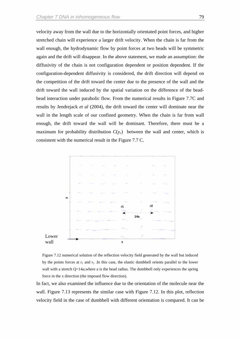
Chapter 7 DNA in inhomogeneous flow 79
velocity away from the wall due to the horizontally orientated point forces, and higher
stretched chain will experience a larger drift velocity. When the chain is far from the
wall enough, the hydrodynamic flow by point forces at two beads will be symmetric
again and the drift will disappear. In the above statement, we made an assumption: the
diffusivity of the chain is not configuration dependent or position dependent. If the
configuration-dependent diffusivity is considered, the drift direction will depend on
the competition of the drift toward the center due to the presence of the wall and the
drift toward the wall induced by the spatial variation on the difference of the bead-
bead interaction under parabolic flow. From the numerical results in Figure 7.7C and
results by Jendrejack et al (2004), the drift toward the center will dominate near the
wall in the length scale of our confined geometry. When the chain is far from wall
enough, the drift toward the wall will be dominant. Therefore, there must be a
maximum for probability distribution C(yc) between the wall and center, which is
consistent with the numerical result in the Figure 7.7 C.
x
y
r1
14a
r2
Figure 7.12 numerical solution of the reflection velocity field generated by the wall but induced
by the points forces at r1 and r2 .In this case, the elastic dumbbell orients parallel to the lower
wall with a stretch Q=14a,where a is the bead radius. The dumbbell only experiences the spring
force in the x direction (the imposed flow direction).
Lower wall
In fact, we also examined the influence due to the orientation of the molecule near the
wall. Figure 7.13 represents the similar case with Figure 7.12. In this plot, reflection
velocity field in the case of dumbbell with different orientation is compared. It can be

Chapter 7 DNA in inhomogeneous flow 80
seen that when molecule orientated smaller or larger than 45o, it will migrate toward
the wall, and hydrodynamic flow will drive the molecule to align with the flow
direction during the process. However, it can be seen in Figure 6.6 in the chapter 6,
molecule has more probability to orientate parallel to the wall. Therefore, the
configuration with smaller angle close to zero should be dominant in the real case,
which indicates the deterministic drift of molecule (near the wall) toward the center.
Figure 7.13 Comparsion of the reflection velocity field generated by the wall but induced by
the points forces at r1 and r2 .In this case, the elastic dumbbell oriented smaller and larger than
45o with the imposed flow direction with a stretch Q= 41 a,where a is the radius of the bead.
Lower wall
Lower wall
B
A

Chapter 7 DNA in inhomogeneous flow 81
In addition, as shown in Figure 7.7, as the increase of the flow strength, the reflection
velocity field will become stronger compared with that at the same position with the
smaller flow strength, since the higher stretched chain induces a stronger reflection
velocity field. Therefore, the depletion layer will be significantly increased as the
increase of the flow strength.
In fact, our explanation is a rather rough approach to migration behavior, especially
the analytical part: the molecule is regarded as the dumbbell model, which indicates
lots of contributions from internal configurations of molecule are not explored.
However, the simple mechanism is still consistent with the simulation results by
Jendrejack et al (2004): Full HI model will predict migration toward the center in the
confined geometry, which displays flow induced evolution of configuration of
polymer chain in an accurate fashion
Chapter 7 DNA in inhomogeneous flow 82
Reference J.J.de Pablo, H.C.Ottiinger , Hydrodynamic Changes of the Depletion Layer of Dilute Polymer
Solutions Near a wall ,AlchE Journal,308,1992
M.Chopra, R.G.Larson, Brownian dynamics simulations of isolated polymer molecules in shear flow
near adsorbin and nonadsorbing surface, J.Rheol.46, 831- 862,2002
R.M.Jendrejack, D.C.Schwartz, J.J.de Pablo, M.D.Graham, Shear-induced migration in flowing
polymer solutions: simulation of long-chain DNA in microchannels, J.Chem Phys,120,2513-2529,2004
Y.H.Seo, O.O.Park, M.S.Chun, The behavior of the velocity enhancement in microcapillary flows of
flexible water-soluable polymers,J.Chem.Eng.Jpn,29,611,1996
L.F, H.Hu, R.G.Larson, DNA configurations and concentration in shearing flow near a glass surface in
a microchannel, J. Rheol.49,127-138,2005
M.Chopra, R.G.Larson, Brownian dynamics simulations of isolated polymer molecules in shear flow
near adsorbing and non adsorbing surfaces , J. Rheol.46,831-862,2002
R.B.Bird, C.F.Curtiss, R.C.Armstrong, O.Hassager, Dynamics of Polymeric Liquids Wiley ,Vol.2,1987

Chapter 8 Conclusion and Future work 83
Chapter 8 Conclusion and Future work
8.1 Conclusion Simulations of dilute DNA solution in equilibrium in free solution and the confined
geometries are performed in Chapter 5. We observed that there is a transition region
for molecule stretch and diffusivity of the chain at H ≈10 RG, where H is the width of
the square channel and RG is the radius of gyration of polymer chain in free-solution.
It indicates that the chain can be considered strong confined when the characteristic
length scale of the confined geometry lowers down to certain value; otherwise, the
chain will behave as it does in the free solution
In Chapter 6, simulations of dilute solution in simple shear flow in confined
geometries are performed. Molecular orientation, molecule stretch and thickness in
velocity gradient direction are examined and the results by Bulk HI model give
qualitative agreements with the newest experimental data (Teixeira et al, 2005).
Tumble dynamics of polymers in the shear flow proposed by Steven Chu is proved
indirectly. In addition, migration behaviour is observed in this case, which is
consistent with the mechanism we motioned in the chapter 7.
In Chapter 7, migration towards the center of microchannel is correctly predicted by
Full HI model. Through the theoretical analysis of dumbbell model and simulation of
bead-spring model, the following conclusions can be made on the migration
beheavior:
a) There is deterministic hydrodynamic drift away from the walls. This is
because highly stretched chain near the wall will generate a hydrodynamic
flow field, which will induce a reflection flow field from the wall to break the
symmetry of hydrodynamic flow and push the chain away from the wall.
b) There is non-completely Brownian drift, which couples with the spatial
variation of configuration-dependent bead-bead hydrodynamic interaction,
away from the centerline
c) The center-of-mass distribution of the steady state will depend on the
competition of those two effects. In our geometry, the deterministic drift term
will be dominant near the wall and the Brownian drift will be dominant near

Chapter 8 Conclusion and Future work 84
the centreline of the channel. Therefore, a maximum is predicted at the
halfway between the wall and center and nonmonotonical distribution of
center-of-mass is predicted. In addition, the depletion layer is predicted to
increase with the increase of flow strength.
8.2 Future Work So far, we have presented simulation results in the microchannel with square cross
section under simple shear flow and pressure-driven flow. Since the dynamics of
polymers in confined geometry are extremely important for many natural and
industrial processes, the following work may be interesting:
a) Different geometries will induce different hydrodynamic flow field from the
boundaries, such as the channel with a triangle cross section has a fundamental
interest for the SEC (Size Exclusion Chromatography) technology. In addition,
the surface pattern in the channel would be interesting to explore for the
purpose of bimolecular sorting.
b) In our project, the surface of the channel has a weaker repulsive potential to
mimic the desorbing surface. In fact, adsorbing surface is subject to more
extensive interests in science and technology.
c) More complex flow patterns are also interesting to consider. For example, a
DNA molecule flowing into micro or nano-porous geometries is a contract
flow, such kind of problem has a fundamental biological interest, eg. How
virus gets though the membrane of cells.
d) Electromagnetic effect is also interesting to be examined. Deep understanding
on how this effect influences the dynamics of biomolecules in the confined
geometries will give lots of fresh ideas to the design of microfludic systems.
e) We are focusing on single molecule dynamics in this project for simplicity. In
fact, the solution is concentrated in most of cases, therefore multi-chain system
with different concentration effects will be interesting to be examined. With
interchain entanglement, the project will become more complex.
f) To accomplish the above ideas, the algorithm needs to be optimized and more
advanced computing resources and techniques are needed.
Appendices 85
Appendices
A-1 Evaluation for Green’s function To evaluate the Green’s function for the confined geometries, we need to set right
boundary condition (2.44).
To get , using Equation (2.42), we can get 'OBv
( ) ( )OB OB j j′ = − ⋅v Ω r r f r (1.1)
For simplicity, we write the explicit expression for Equation (1.1)
,1 111 12 13
,2 21 22 23 2
31 32 33 3,3
OB OB OBOB
OB OB OBOB
OB OB OBOB
v fv f
fv
′⎛ ⎞ ⎛ ⎞Ω Ω Ω ⎛ ⎞⎜ ⎟ ⎜ ⎜ ⎟′ = Ω Ω Ω ⋅⎜ ⎟ ⎜ ⎜ ⎟
⎜ ⎟⎜ ⎟ ⎜ ⎟Ω Ω Ω′ ⎝ ⎠⎝ ⎠⎝ ⎠
⎟⎟ (1.2)
Here we always use instead of .from Equation (2.33), we know: RPYΩ OBΩ
1 2 2
( )( )1( )8
j jRPYj
S j j
C Cπη
⎡ ⎤− −⎢ ⎥− = +⎢ ⎥− −⎣ ⎦
r r r rΩ r r I
r r r r (1.3)
Here rj is the point where the point force f(rj) generates a velocity perturbation
at r
'OBv
i ,so rj can be regarded as the source point and ri should be your observation point
or measurement point for velocity perturbation.
Here I is a unit tensor and (r- rj)(r-rj) is a dyadic product as follows:
2
2
2
( ) ( )( ) ( )(( )( ) ( )( ) ( ) ( )(
( )( ) ( )( ) ( )
j j j j
j j j j j j j
j j j j j
))
jx x x x y y x x zy y x x y y y y z zz z y y z z y y z z
⎛ ⎞− − − − −⎜ ⎟
− − = − − − − −⎜ ⎟⎜ ⎟− − − − −⎝ ⎠
r r r rz
(1.4)
Then we can write each component for the velocity perturbation 'OBv
,1 11 1 12 2 13 3
21 2
1 1 2 2
( ) ( )( ) ( )( )18
OB OB OBOB
j j j j
S j j
v f f f
3jx x f x x y y f x x z z fC f C
πη
′ = Ω ⋅ +Ω ⋅ +Ω ⋅
⎡ ⎤− + − − + − −⎢ ⎥= +⎢ ⎥− −⎣ ⎦
r r r r
(1.5)

Appendices 86
,2 21 1 22 2 23 3
21 2
1 2 2 2
( )( ) ( ) ( )( )18
OB OB OBOB
j j j j j
S j j
v f f f
3x x y y f y y f y y z z fC f C
πη
′ = Ω ⋅ +Ω ⋅ +Ω ⋅
⎡ ⎤− − + − + − −⎢ ⎥= +⎢ ⎥− −⎣ ⎦
r r r r
(1.6)
,3 31 1 32 2 33 3
21 2
1 3 2 2
( )( ) ( )( ) ( )18
OB OB OBOB
j j j j j
S j j
v f f f
3x x z z f z z y y f z z fC f C
πη
′ = Ω ⋅ +Ω ⋅ +Ω ⋅
⎡ ⎤− − + − − + −⎢ ⎥= +⎢ ⎥− −⎣ ⎦
r r r r
(1.7)
To use those equations, we take an assumption that the beads are well separated with
each other.
After setting the boundary condition, we can get velocity perturbation field, then we
can evaluate the Green’s function for the wall numerically based on the grid.
11
211
31
1W
WW
Wf
⎛ ⎞Ω⎜ ⎟
′Ω =⎜ ⎟⎜ ⎟Ω⎝ ⎠
v (1.8)
Where 1,2,3 is the three directions of the vector. The second and third column of the
can be get in the similar way by applying the point force in the direction 2,
3, respectively. Here is a trick: when we evaluate each column of the Green’s
function, we need to set the point forces in other direction to zero and the point force
in the corresponding direction to a unit point force. During the evaluation, the point
force in the corresponding direction can be arbitrary value, because this Stokes
equation is a linear equation, the magnitude of the force will be scaled up in the final
stage. In addition, from another point of view, the Green’s function here should only
depend on the geometry, and is independent of the direction and magnitude of the
point force. The magnitude of the point force will only influence the resulting velocity
perturbation field, but when we evaluate the Green’s function, this force will be
removed anyway.
( , )WjΩ x x
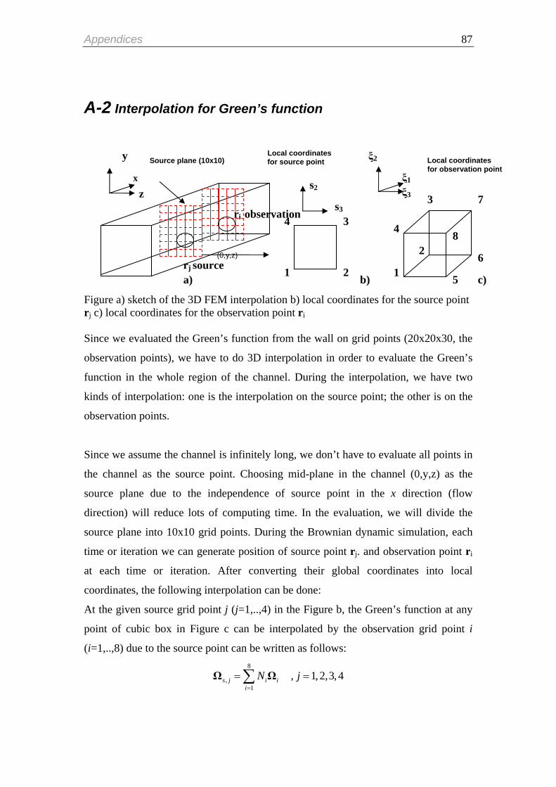
Appendices 87
A-2 Interpolation for Green’s function
y ξ2Local coordinates
Local coordinates Source plane (10x10) for source point for observation point
Figure a) sketch of the 3D FEM interpolation b) local coordinates for the source point rj c) local coordinates for the observation point ri Since we evaluated the Green’s function from the wall on grid points (20x20x30, the
observation points), we have to do 3D interpolation in order to evaluate the Green’s
function in the whole region of the channel. During the interpolation, we have two
kinds of interpolation: one is the interpolation on the source point; the other is on the
observation points.
Since we assume the channel is infinitely long, we don’t have to evaluate all points in
the channel as the source point. Choosing mid-plane in the channel (0,y,z) as the
source plane due to the independence of source point in the x direction (flow
direction) will reduce lots of computing time. In the evaluation, we will divide the
source plane into 10x10 grid points. During the Brownian dynamic simulation, each
time or iteration we can generate position of source point rj. and observation point ri
at each time or iteration. After converting their global coordinates into local
coordinates, the following interpolation can be done:
At the given source grid point j (j=1,..,4) in the Figure b, the Green’s function at any
point of cubic box in Figure c can be interpolated by the observation grid point i
(i=1,..,8) due to the source point can be written as follows: 8
,1
, 1, 2,3, 4s j i ii
N j=
= =∑Ω Ω
x ξ1
z ξ3
1
2
3
4
5
6
7
8
1 2
4
s2
s3ri observation 3
(0,y,z)
a) rj source
b) c)

Appendices 88
where Ni is the shape function for the observation point i, which can be defined as
follows:
1 1 2
2 1 2
3 1 2
4 1 2
5 1 2
6 1 2
7 1 2
8 1 2
1 (1 )(1 )(1 )81 (1 )(1 )(1 )81 (1 )(1 )(1 )81 (1 )(1 )(1 )81 (1 )(1 )(1 )81 (1 )(1 )(1 )81 (1 )(1 )(1 )81 (1 )(1 )(1 )8
N
N
N
N
N
N
N
N
3
3
3
3
3
3
3
3
ξ ξ ξ
ξ ξ ξ
ξ ξ ξ
ξ ξ ξ
ξ ξ ξ
ξ ξ ξ
ξ ξ ξ
ξ ξ ξ
= − − −
= + − −
= + + −
= − + −
= − − +
= + − +
= + + +
= − + +
Where ξ1, ξ2, ξ3 is the local coordinates for the observation points shown in the Figure
c. It can be seen that the interpolation for observation point is a 3D interpolation,
while the interpolation for the source point is actually 2D interpolation due to the
infinite long effect of the channel in the flow direction we mentioned above.
Since we get the Green’s function of any observation point ri in the cubic box in
Figure c due to the source point at grid point j, if the source point rj in Figure b is in
the square but not at the grid point, the Green’s function can be interpolated as
follows:
4
, ,1
( , )i j s j s jj
N=
= ∑Ω r r Ω
where Ns,j is the shape function for the source point rj ,which can be defined as
follows:
,1 3 2
,2 3 2
1 (1 )(1 )41 (1 )(1 )4
s
s
N s
N s
= − −
= + −
s
s
Appendices 89
,3 3 2
,4 3 2
1 (1 )(1 )41 (1 )(1 )4
s
s
N s
N s
= + −
= − +
s
s
Where s2,s3 is the local coordinates for the source points.
Finally, is the approximation of the Green’s function for observation point r( , )i jΩ r r i
due to the point force at rj. To increase the accuracy of evaluation of the Green’s
function, decreasing the mesh size of each gird or increasing the discretization of the
space is a choice, but the computing time will be significantly increased, since we
have to locate the positions of source point and observation point first each time
before starting the interpolation.
A-3 Chebyshev polynomial approximation
T= ⋅D B B
D should be the symmetric semi-definite matrix, whose decomposition B in the above
equation always can be efficiently solved by Cholesky decomposition. However,
sometimes it fails during the simulation, so we can’t make sure all eigenvalues of the
diffusion tensor generated during the simulation is larger or equal to zero.
In addition, the decomposition of the diffusion tensor D is computational expensive
and scales with N3, while the Chebyshev decomposition scales with N2.5(Kroger et
al,2000; Jendrejack et al 2000) .Therefore, we introduce a method named Chebyshev
polynomial approximation by Fixman (1986). B can be approximated by the
following expression (Press et al, 1992):
11
1( )2
L
k kk
c D−=
= ∑B T 1c−
l
(2.1)
where
1 12a b
l l
d d
+ −
= += −
0
1
1
T = IT D IT C C C
(2.2)

Appendices 90
with
max min
2ad
λ λ=
− (2.3)
max min
max minad λ λ
λ λ+
=−
(2.4)
Where maxλ and minλ is the maximum and minimum of D; ck is the Chebyschev
coefficient , which can be obtained by the following way (Jendrejack et al,2000):
1
1
cos[ ( 1/ 2) / ]L
Lj kj
k
c L a a k Lα π−+ −
=
= + −∑ (2.5)
Where
( ) / 2( ) / 2
2cos[ ( 1)( 1/ 2) / ]
a b
b aLkj
a d da d d
j k Lα π
+
−
= += −
= − −
Here L is approximation degree. For a fixed L, Equation (2.1) is a polynomial which
can approximate B in the interval [ maxλ , minλ ].This approximation may be not better
than other approximation from a point of view of accuracy, but it can be truncated to
lower degree of M<L in a graceful way. It is difficult to find the minimal value of L,
50 are typical value used in our case (Press et al, 1992).
Because is our interest, whose polynomial y can be approximated by the same approach:
d⋅B w
11
L
k Kk
d c −=
= ⋅ =∑y B w x (2.6)
0 d=x w (2.7)
1 1 d= ⋅x T w (2.8) 1 12l l 1l+ −= ⋅ −x T x x (2.9)
The Chebyshev expansion is only valid within the chosen eigenvalue range;
sometimes, a violation of the eigienvalue limits could happen. A method for error
evaluation is proposed by R.M.Jendrejack et al (2004). Using Equation (2.6) and
Equation (2.7) we can get
lim[ ]L
d d→∞
⋅ = ⋅ ⋅y y w D w (2.10)
Assuming the eigenvalues we are using are valid. A relative error Ef can be defined
as follows(Jendrejack,2004):

Appendices 91
f
d dE
d d⋅ − ⋅ ⋅
=⋅ ⋅
y y w D ww D w
(2.11)
Here, we give a initial guess of the eigenvalues of diffusion tensor D first ,then check
if the error is acceptable. If it is not, we can compute another set of eigenvalues until
the error requirement is satisfied.
In this way, we check the extent of violation of the fluctuation-disspation theorem is
small enough to get a desired accuracy.
Reference: M.Kroger, A.Alba-Perez, M.Laso,H.C.Ottinger, Variance reduced Brownian simulation of a bead-
spring chain under steady flow considering hydrodynamic interaction
effects,J.Chem.Phys.113,4767,2000
R. M. Jendrejack, M. D. Graham, and J. J. de Pablo, Hydrodynamic interactions in long chain
polymers: Application of the Chebyshev polynomial approximation in stochastic simulations, J. Chem.
Phys.113,2894, 2000
Jendrejack, R. M., Multiscale Simulations of Dilute-Solution Macromolecular Dynamics in
Macroscopic and Microscopic Geometries, Doctoral dissertation ,2003
W. Press, S. A. Teukolsky, W. T. Vetterling, and B. P. Flannery, Numerical Recipes in Fortran, 2nd
ed. Cambridge University Press, Cambridge,1992
M. Fixman, Construction of Langevin Forces in the Simulation of Hydrodynamic Interaction,
Macromolecules ,19, 1204,1986.
A-4 Construction of positive definite Hydrodynamic interaction tensor As we mentioned before, Oseen tensor in free solution will lead to unphysical
properties of diffusion tensor, e.g. negative translational diffusion coefficients .The
main origin is the treatment of segments as point sources of friction according to the

Appendices 92
Oseen tensor (Yamakawa,1970). Hence RPY tensor is introduced to guarantee the
diffusion tensor to be a positive-semidefinite for all the chain configurations.
Problem happens when we add the correction term from the geometry to
the Green’s function. During the simulation, the diffusion tensor D could become
non-positive at some points, at which the program will break down. In order to keep
the positive-semidefinite properties of diffusion tensor, we have to make some
modifications to the diffusion tensor D. In the following, we will explain this issue.
( , )WjΩ r r
First, we check the positive definiteness of (the hydrodynamic interaction tensor
for a point force at r
ijD
j) by determining the eigenvalues of 3×3 matrix. If is non-
positive, it needs to be modified. For computational efficiency, one can set ,
where c<1 until becomes positive-definite. Here c could be a constant, but if c can
be designed to be a function of relative distance between source point and observation
point, the error due to modification of the diffusion tensor can be reduced to some
extent (Jendrejack, et al, 2004).
ijD
ij iic=D D
ijD
Reference H. Yamakawa, Transport properties of Polymer Chains in Dilute Solution: Hydrodynamic Interaction,
J. Chem. Phys.53, 436, 1970
R.M.Jendrejack, D.C.Schwartz, J.J.de Pablo, M.D.Graham, Shear-induced migration in flowing
polymer solutions: simulation of long-chain DNA in microchannels, J.Chem Phys,120,2513-2529,2004
Top Related