


Languages
Pages
Legal


Linear Algebra
An Introduction to Linear Algebra for Pre-Calculus Students
by
Tamara Anthony Carter
Adjunct Professor of Mathematics, University of North Texas
Richard A. Tapia
Noah Harding Professor, Computational and Applied Mathematics
Director, Center for Excellence and Equity in Education
Anne Papakonstantinou
Director, Rice University School Mathematics Project
Rice University
May 1995

Copyright
Tamara Lynn Anthony
1995
Contents
Preface v
1 Introduction to Matrices 1
2 Addition of Matrices 11
3 Multiplication of Matrices 18
4 Equations 33
4.1 Coding . . . . . . . . . . . . . . . . . . . . . . . . . . . . . . . . 43
5 Determinants 54
5.1 Expansion by Minors . . . . . . . . . . . . . . . . . . . . . . . . 56
5.2 Using Gaussian Elimination . . . . . . . . . . . . . . . . . . . . . 58
5.3 Inverses and Solutions to Systems . . . . . . . . . . . . . . . . . 60
5.4 De�nition of the Determinant . . . . . . . . . . . . . . . . . . . . 62
6 Consistent and Inconsistent Systems 68
First Review 75
7 Markov Chains 80
8 Least Squares Approximation 95
8.1 Proof of Normal Equations . . . . . . . . . . . . . . . . . . . . . 107
iii
9 Eigenvalues and Eigenvectors 114
10 Numerical Challenges 132
10.1 Operation Counts . . . . . . . . . . . . . . . . . . . . . . . . . . 136
Second Review 140
11 Tests 143
11.1 Matrix Test 1A . . . . . . . . . . . . . . . . . . . . . . . . . . . . 143
11.2 Matrix Test 1B . . . . . . . . . . . . . . . . . . . . . . . . . . . . 145
11.3 Matrix Test 1C . . . . . . . . . . . . . . . . . . . . . . . . . . . . 147
11.4 Matrix Test 2A . . . . . . . . . . . . . . . . . . . . . . . . . . . . 150
11.5 Matrix Test 2B . . . . . . . . . . . . . . . . . . . . . . . . . . . . 152
12 Solutions 154
12.1 Solutions to Introduction - Problems from page 8 . . . . . . . . . 154
12.2 Solutions to Addition - Problems from page 15 . . . . . . . . . . 161
12.3 Solutions to Multiplication - Problems from page 30 . . . . . . . 170
12.4 Solutions to Systems of Equations - Problems from page 51 . . . 183
12.5 Solutions to Determinants - Problems from page 64 . . . . . . . . 188
12.6 Solutions to Consistent and Inconsistent - Problems from page 74 192
12.7 Solutions to First Review from page 75 . . . . . . . . . . . . . . 193
12.8 Solutions to Markov Chains - Problems from page 90 . . . . . . . 199
12.9 Solutions to Least Squares - Problems from page 110 . . . . . . . 202
12.10 Solutions to Eigenpairs - Problems from page 130 . . . . . . . . . 205
12.11 Solutions to Second Review from page 140 . . . . . . . . . . . . . 206
12.12 Solutions to Matrix Test 1A . . . . . . . . . . . . . . . . . . . . 208

iv
12.13 Solutions to Matrix Test 1B . . . . . . . . . . . . . . . . . . . . . 210
12.14 Solutions to Matrix Test 1C . . . . . . . . . . . . . . . . . . . . . 212
12.15 Solutions to Matrix Test 2A . . . . . . . . . . . . . . . . . . . . 214
12.16 Solutions to Matrix Test 2B . . . . . . . . . . . . . . . . . . . . . 215
Bibliography 217
Index 218

Preface
This book is an introduction to linear algebra for pre-calculus students. It is a stand-
alone unit in the sense that no prior knowledge of matrices is assumed. Students with
experience in general mathematics, up to and including Algebra I, should be able to
comprehend the material. However, most students have not had experience with the
topics in the latter chapters, so the pace of the course should allow for the students to
spend extra time with these chapters. We begin with chapters that explain the matrix
operations of addition, subtraction, scalar multiplication, and matrix multiplication.
These topics are covered in most pre-calculus texts that are currently in use. This
unit also allows the students to explore the notions of inverse, determinant, and
consistent and inconsistent systems; these topics are covered in some pre-calculus text
books. Our unit also provides the students with an introduction to Markov chains,
curve �tting, eigenpairs, and some of the numerical challenges that are encountered
when matrices are used to solve real-world problems. These latter topics are rarely
addressed in pre-calculus texts. The unit was created from elementary principles with
signi�cant input from Rice University faculty and students. Various current texts,
recommendations from the National Council of Teachers of Mathematics (NCTM),
and the Texas essential elements were examined in order to determine which topics
should and should not be included in this text.
The state of Texas signi�cantly in uences the content of pre-college text books,
because a book that is approved for adoption in Texas has a large potential market.
In order for a book to be adopted in Texas, all of the \essential elements" for that
course must be covered in the text. Essential element 4B for Algebra II states that
students should be able to \use augmented matrices by hand or by computer to

vi
solve two- or three-variable linear systems." Essential element 3I for Elementary
Analysis states that students should be able to \solve matrix equations and real-
world problems whose solutions involve matrix equations." According to essential
element 3H for Elementary Analysis, students should be able to \solve a system of
equations or inequalities using graphing techniques and apply [them] in real-world
situations" (Houston Independent School District Scope and Sequence Grades 9-12,
1992). (This text does not address essential element 3H because only two-dimensional
problems can be solved with graphing techniques and \real world problems" require
many more dimensions.) Since these are the only requirements concerning matrices
for Texas high-school mathematics books, many books meet these requirements but
do not really give the students an adequate understanding of linear algebra. It is true
that a college linear algebra text would contain ample detail, but few pre-calculus
students have the mathematical maturity necessary to read these texts.
Since most pre-calculus texts only touch on the subject of matrices, one might
question the need for a more in-depth study of linear algebra at the pre-calculus
level. The NCTM has recognized this need and stated that \matrices and their
applications" should receive \increased attention" in high school (Curriculum and
Evaluation Standards for School Mathematics, 1989, p. 126). It also could be argued
that linear algebra is as important as calculus to many engineers and other scientists.
The introduction of linear algebra at the pre-calculus level would give the students
a knowledge base on which to build when they study linear algebra in college. The
arrays that are studied in linear algebra are of vital importance to computer pro-
grammers and computer users. Linear algebra is also central to the computational
and mathematical sciences.
In The Psychology of Learning Mathematics, Richard Skemp states \: : :the learn-
ing of mathematics, especially in its early stages and for the average student, [is] very

vii
dependent on good teaching" (1987, p. 21). Unfortunately, many teachers have not
had much experience, and do not feel entirely comfortable, with linear algebra, so it
is di�cult for them to teach more than just the procedures of matrix manipulation.
Therefore, we have attempted to write this unit so that the students can directly
access the material. Since discussions add to, and strengthen, one's understanding
of a topic, thought-provoking questions and their answers are provided at the end of
each chapter to spark class discussions. To help the teacher, complete solution steps
have been provided in addition to the solutions where appropriate.
Skemp also states that \concepts of a higher order than those which people already
have cannot be communicated to them by a de�nition [alone], but only by arranging
for them to encounter a suitable collection of examples" (1987, p. 18). For this
reason, most new concepts in this unit are presented with an example that builds on
the intuition of the student. Then the formal de�nition is given, and other examples
follow to clarify the concept. This helps motivate the students because they can
immediately see a use for the concept. It also gives the concept a foundation in the
mind of the student. Although the notion of building concepts in this manner seems
logical, few text books utilize this approach.
Because many books teach procedures rather than concepts, the students do not
receive enough information to expand beyond the examples in the book. For example,
some books teach methods which apply only to the special case of 2 by 2 matrices
when they address the notions of inverse and determinant. However, this text presents
methods for �nding inverses and determinants of square matrices of any size. Since
the students learn the concepts and these general methods, their knowledge is not
restricted by the examples in the book.
Because computers are essential to modern society, computer programming as-
signments are included at the end of the �rst three chapters as a means to help the

viii
students solidify their knowledge of matrices. In some of the later chapters, students
are encouraged to use calculators to help them explore matrices so that they are not
tied to problems that can be reasonably computed by hand. The students are not
asked to use a particular computer language or a particular calculator, but the code
for working programs are provided for the teachers in BASIC and PASCAL.
When new topics are introduced in this unit, they are tied, as much as possible,
to previous topics. This is in an attempt to allow the students to appreciate linear
algebra as a whole rather than view each chapter as a separate entity. For example,
solutions to systems of equations are computed using Gaussian elimination, Gauss-
Jordan elimination, and Cramer's rule. The text demonstrates to the students that a
form of Gaussian elimination can be used, as an alternative to expansion by minors,
to compute determinants. We use these two methods of computing the determinant
to discuss e�ciency of algorithms so that the students know that �nding the correct
answer is not the only concern. The students are also told that the determinant of
a matrix is the same as the product of its eigenvalues. The relationship between
the steady state of a transition matrix and eigenpairs is also demonstrated to the
students. These ties and others provide the students with di�erent perspectives from
which to view problems.
Most texts do not mention Markov chains, even though they are well within
the grasp of pre-calculus students. The NCTM believes that \in grades 9-12, the
mathematics curriculum should include topics from discrete mathematics so that all
students can represent graphs, matrices, sequences, and recurrence relations" (1989,
p. 176). Hopefully, this chapter will catch the attention of the student because a
Markov chain is a real application of matrices rather than a contrived book example.
This chapter also o�ers the student a glance into the fascinating world of probability.

ix
Curve �tting is another interesting application of matrix equations, and it can be
used immediately in the life of a pre-calculus student. Most pre-calculus students
take a laboratory science in which they could use curve �tting to analyze their data.
This cross-discipline application also helps the students to view mathematics as a
useful tool rather than just a subject to take in school. The NCTM believes that \in
grades 9-12, the mathematics curriculum should include the continued study of data
analysis and statistics so that all students can use curve �tting to predict from data"
(1989, p. 167). Curve �tting is also a bridge between the �elds of mathematics and
statistics.
Eigenpairs are essentially never found in pre-calculus text books, but they have a
wide range of physical applications that could interest students. The computational
methods taught in this unit build naturally on previous topics in the text. Because
the computation of eigenpairs quickly increases in di�cultly as the size of the matrix
increases, only simple examples are given in this unit. However, students are intro-
duced to the concept of matrices and to many of their applications, so they will have
a foundation on which to build when they study eigenpairs in college.
The chapter entitled \Numerical Challenges" is important to the students' overall
knowledge even though the students are not asked to perform computations. This
chapter reminds students that the world is not solely comprised of pretty book ex-
amples. It also helps dispel the notion that mathematics is only about learning what
other people already know. It is good for students to know that many important chal-
lenges remain in mathematics and that bright young minds are needed to research
these topics.
This entire unit was written so that pre-calculus teachers and students will have a
text that clearly and accurately explains the introductory concepts of linear algebra.
It explores the topics that are currently addressed in pre-calculus courses, but em-

x
phasizes concepts rather than than just procedures. This unit also provides students
with many more real-world linear algebra topics to explore than are presented in cur-
rent texts. It is hoped that this unit will not only help students understand linear
algebra, but will also spark an interest in, and an appreciation for, the mathematical
sciences.
How can it be that mathematics, being after all a product of human
thought which is independent of experience, is so admirably appropriate
to the objects of reality? - Albert Einstein
It truly is beautiful that the abstract concepts of mathematics can be used to
model the world around us. This is astounding because the laws of mathematics were
not created with the universe, but have been de�ned by mankind over the centuries.
These laws model the world so well, that people often fail to distinguish between
the real situation and the mathematical model that is being used to study it. For
example, because matrices can be used to represent a system of equations which
model the real world, people often think that the solution to the system will also
be the solution to the real-world problem. However, the solution is only as good as
the model that was used to represent the problem. Since the world is so complex,
mathematical models cannot accurately model every detail of the universe. However,
they may come amazingly close and help illuminate many of the mysteries of the
universe.
1
Chapter 1
Introduction to Matrices
If you were asked for your weight in pounds, you would use a real number such as 140
to answer the question. If you were asked for your height in inches, you would answer
with another real number such as 66.5. If we asked these questions to everyone in the
class, we would want some way to know which weight goes with which height. One
way to organize this data is to use an ordered pair. We could represent your weight
and height with the ordered pair (140, 66.5). This is called an ordered pair because
we always list the information in the same order. In other words, we list weight
�rst and then height in every pair of numbers, so (140, 66.5) would be di�erent from
(66.5, 140). The elements are the individual pieces of information. Elements are
also referred to as entries or components. In this book, we will only use real numbers
as elements. The elements of this ordered pair are 140 and 66.5. We could also ask
you for your age in years and append that information so that we have the ordered
triple (140, 66.5, 18). We could ask you for n pieces of information, where n is any
counting number. If we arrange the n pieces of information in a speci�c order, we
call it an ordered n-tuple. In general, lists of ordered information are called vectors.
If we write them in rows, as we did above, we call them row vectors. If we write
them in columns, such as
264 140
66:5
375 and
2666664
140
66:5
18
3777775; we call them column vectors.
De�nition 1.1 A real n�vector is an ordered n-tuple of real numbers.
The real numbers are called the elements of the vector.

2
Since we are only working with real numbers in this book, we will drop the word
real when referring to vectors. When it is not important to specify how many elements
are in the vector, we drop the quali�er n:
Remark 1 Did you notice that we used parentheses on some vectors
and brackets on others? Actually, both are accepted notations, but we
will use brackets for consistency throughout the rest of the book.
Remark 2 Sometimes you will see the elements of a row vector sepa-
rated by commas. Commas are not necessary unless confusion can arise
without the use of commas.
If you were asked to add, subtract, or multiply real numbers, you would know
what to do. If we are going to use vectors to help us organize our information, we
also need rules for vectors so that when we add, subtract, or multiply vectors, we
get the same solutions as if we had not organized our data this way. Remember that
vectors are simply tools that we use to display information in an organized manner.
Therefore, we do not want our solutions to change just because we organized our
data into a vector. As we study this book, we will learn more about how to perform
mathematical operations with vectors.
Consider the following information:
The Cardinals win seven, lose six, and tie one. The Eagles win �ve, lose
eight, and tie one. The Falcons win two, lose twelve, and have no ties.
The Owls win nine, lose �ve, and have no ties.
We can represent this data using the four vectors
�7 6 1
�;
�5 8 1
�;�
2 12 0
�; and
�9 5 0
�: However, it would be nice if we could combine all
these vectors together into one set of data. If we consider each vector as one row of
an array, then we will have all our data in one arrangement.

3
De�nition 1.2 A real matrix is an arrangement of real numbers into
rows and columns.
The real numbers are called the elements of the matrix.
Since we are only working with real numbers in this book, we also will drop the
word real when referring to matrices. Notice that a vector is a special matrix that has
only one row or one column. When we organize our vectors into a matrix, it could
look like this: 26666666664
7 6 1
5 8 1
2 12 0
9 5 0
37777777775
Basically, we have all of our information organized into one arrangement called a
matrix.
We have all the appropriate numbers in our matrix, but if we want to know which
numbers correspond to which team, we have to look back at our paragraph. For this
reason, we often label our matrices (plural of matrix). Labels are not a formal part
of the matrix, but they are very useful. Our matrix could look like this after it has
been labeled:
C
E
F
O
W L T26666666664
7 6 1
5 8 1
2 12 0
9 5 0
37777777775
Just by looking at this matrix, we can tell that the Owls won the most games and
the Falcons lost the most. One of the advantages of matrices is that information is
easier to see and compare than when it is not organized into a matrix.
4
This matrix is referred to as a 4 by 3 matrix (often written 4�3) because there
are 4 rows and 3 columns. Therefore, the dimensions of this matrix are 4 by 3. The
dimensions of a matrix tell you the \size" of the matrix because they tell you the
number of rows and columns in the matrix. By convention, we list the number of
rows before the number of columns.
De�nition 1.3 The dimensions of a matrix are the number of rows
and columns (listed in that order) of the matrix.
Each element of the matrix is named according to its position. Typically, capital
letters represent matrices and small letters with subscripts represent elements in the
matrix. Since vectors can be considered to be matrices with only one row or one
column, they could be labled with capital letters also. However, vectors are usually
represented by small letters. If we name the above matrix A, the element 6 is in the
position a12 (read a one two) because it is in row 1 and column 2. Also by convention,
we list the row number of the element before the column number. An element in row
i and column j would be denoted by aij: This gives us a compact way to refer to
speci�c elements of a matrix.
Remark 3 Although some mathematicians make a distinction between
a 1 by 1 matrix, a 1-vector, and a real number, we will not make any
distinction between them and will treat them exactly the same.
5
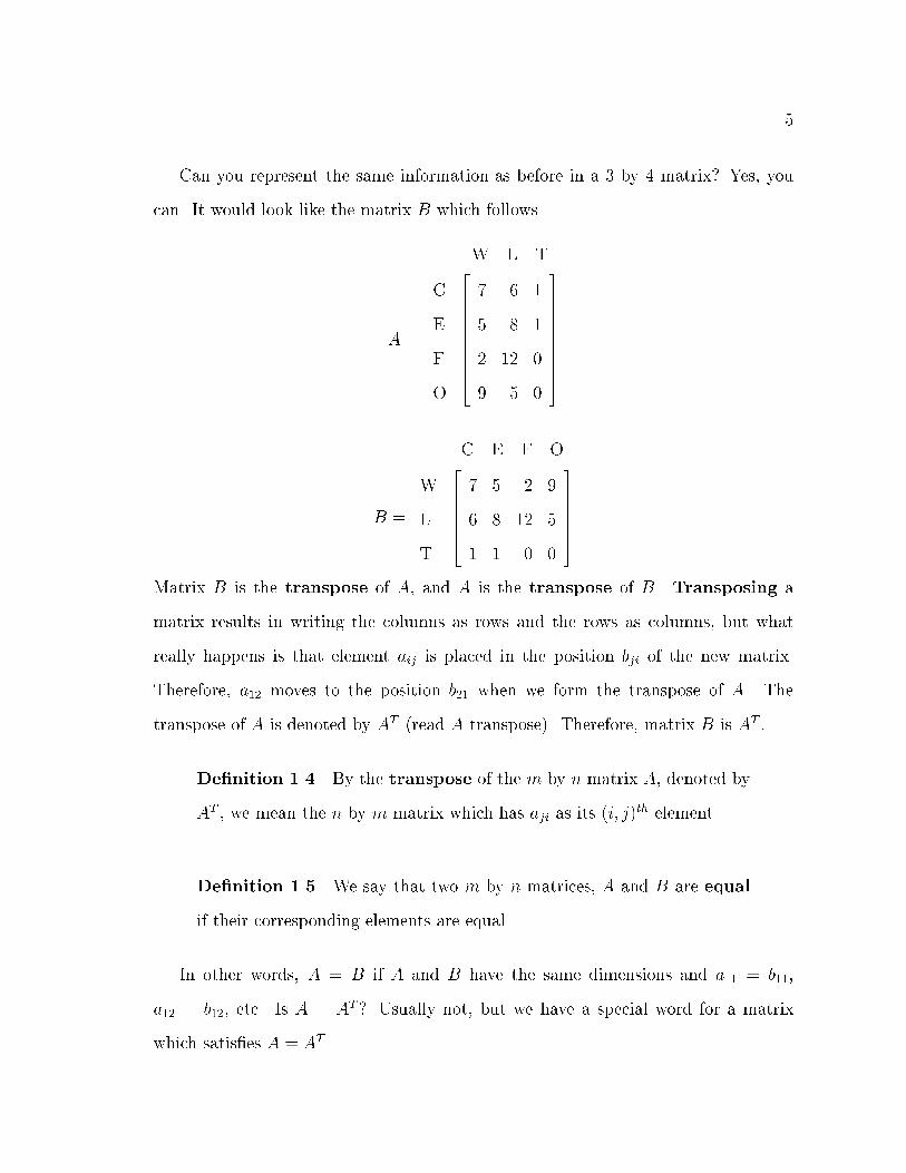
Can you represent the same information as before in a 3 by 4 matrix? Yes, you
can. It would look like the matrix B which follows.
A =
C
E
F
O
W L T26666666664
7 6 1
5 8 1
2 12 0
9 5 0
37777777775
B =
W
L
T
C E F O2666664
7 5 2 9
6 8 12 5
1 1 0 0
3777775
Matrix B is the transpose of A, and A is the transpose of B. Transposing a
matrix results in writing the columns as rows and the rows as columns, but what
really happens is that element aij is placed in the position bji of the new matrix.
Therefore, a12 moves to the position b21 when we form the transpose of A. The
transpose of A is denoted by AT (read A transpose). Therefore, matrix B is AT:
De�nition 1.4 By the transpose of the m by n matrix A, denoted by
AT , we mean the n by m matrix which has aji as its (i; j)
th element.
De�nition 1.5 We say that two m by n matrices, A and B are equal
if their corresponding elements are equal.
In other words, A = B if A and B have the same dimensions and a11 = b11;
a12 = b12; etc. Is A = AT ? Usually not, but we have a special word for a matrix
which satis�es A = AT .

6
De�nition 1.6 A matrix is said to be symmetric if A = AT:
Observe that the following matrix is symmetric:
S =
26666666664
9 2 5 1
2 7 0 8
5 0 4 6
1 8 6 3
37777777775:
Notice that aij = aji for all i and j; as is true for all symmetric matrices. Symmetric
matrices are easy to spot because if you draw a line down the main diagonal (from 9
to 3 in this matrix), then the two halves are mirror images of each other. Symmetric
matrices have many special qualities that will be used when you study matrices in
more detail. The matrix S, given above, has another special property; it is a square
matrix because S has the same number of rows as columns. Notice that S is a 4 by 4
square matrix. We said that the main diagonal for S runs from 9 to 3. For any square
matrix, themain diagonal runs from the upper left corner to the lower right corner.
De�nition 1.7 We say that an m by n matrix is square if m = n.
Questions
1. For a matrix A, what is the transpose of AT ?
2. Does a symmetric matrix have to be square?
3. Are all square matrices symmetric?
Answers
1. Let us choose a generic matrix. We need to be careful when choosing a generic
matrix. Vectors and square matrices often have special properties, so we will
7
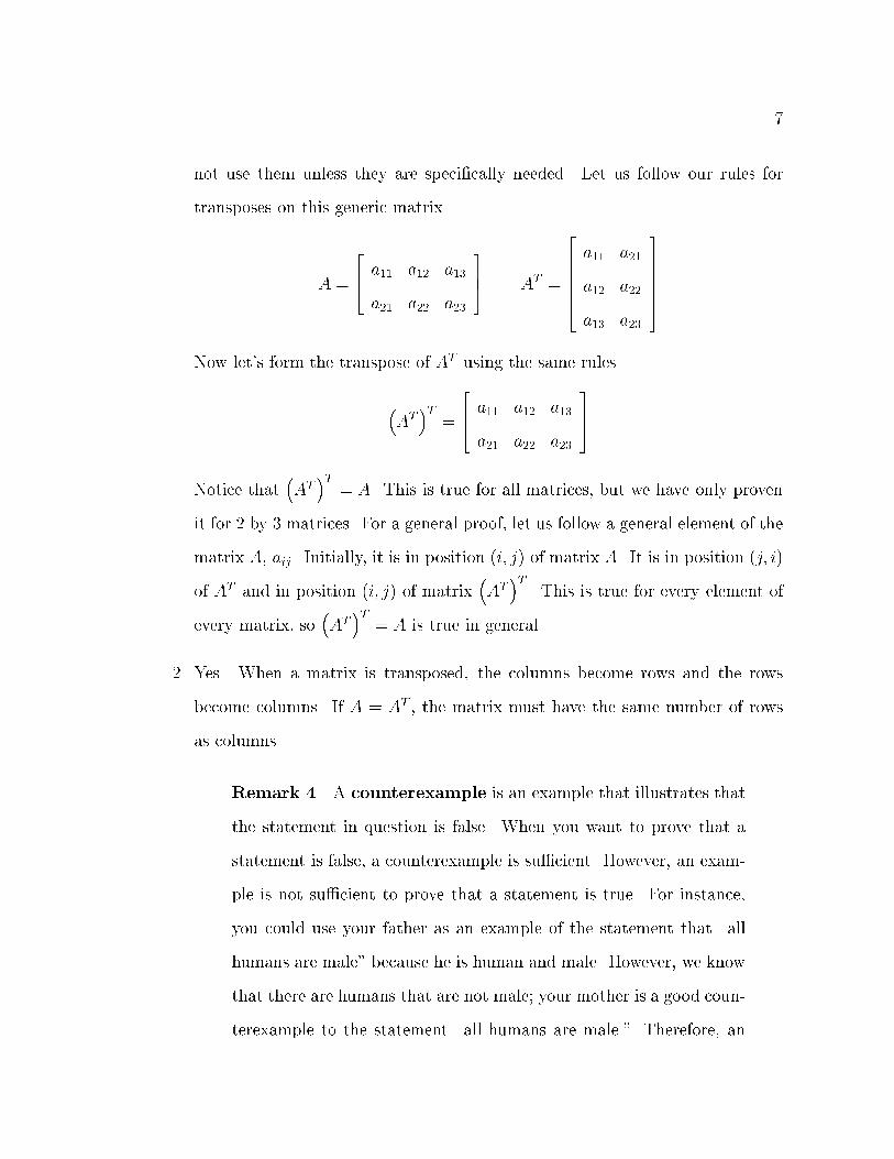
not use them unless they are speci�cally needed. Let us follow our rules for
transposes on this generic matrix.
A =
264 a11 a12 a13
a21 a22 a23
375 A
T =
2666664
a11 a21
a12 a22
a13 a23
3777775
Now let's form the transpose of AT using the same rules.
�AT�T
=
264 a11 a12 a13
a21 a22 a23
375
Notice that�AT�T
= A. This is true for all matrices, but we have only proven
it for 2 by 3 matrices. For a general proof, let us follow a general element of the
matrix A, aij. Initially, it is in position (i; j) of matrix A. It is in position (j; i)
of AT and in position (i; j) of matrix�AT�T. This is true for every element of
every matrix, so�AT�T
= A is true in general.
2. Yes. When a matrix is transposed, the columns become rows and the rows
become columns. If A = AT , the matrix must have the same number of rows
as columns.
Remark 4 A counterexample is an example that illustrates that
the statement in question is false. When you want to prove that a
statement is false, a counterexample is su�cient. However, an exam-
ple is not su�cient to prove that a statement is true. For instance,
you could use your father as an example of the statement that \all
humans are male" because he is human and male. However, we know
that there are humans that are not male; your mother is a good coun-
terexample to the statement \all humans are male." Therefore, an
8
example cannot be used to prove that a statement is true. You would
have to show that it is true for ALL cases. For our example, you
would have to establish in some way that EVERY human is male.
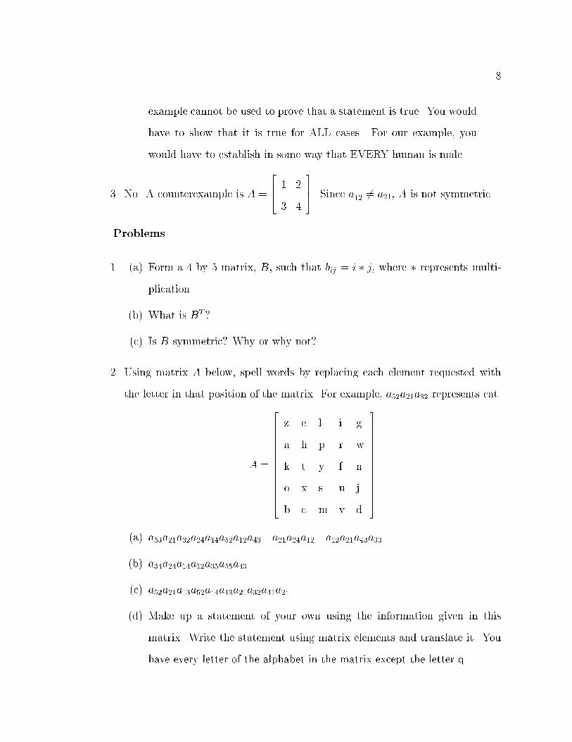
3. No. A counterexample is A =
264 1 2
3 4
375. Since a12 6= a21; A is not symmetric.
Problems
1. (a) Form a 4 by 5 matrix, B; such that bij = i � j; where � represents multi-
plication.
(b) What is BT ?
(c) Is B symmetric? Why or why not?
2. Using matrix A below, spell words by replacing each element requested with
the letter in that position of the matrix. For example, a52a21a32 represents cat.
A =
266666666666664
z e l i g
a h p r w
k t y f n
o x s u j
b c m v d
377777777777775
(a) a53a21a32a24a14a52a12a43 a21a24a12 a12a21a43a33
(b) a34a24a14a12a35a55a43
(c) a52a21a13a52a44a13a21a32a41a24
(d) Make up a statement of your own using the information given in this
matrix. Write the statement using matrix elements and translate it. You
have every letter of the alphabet in the matrix except the letter q.

9
3. (a) Put the following information into a 3 by 2 matrix and attach labels:
The Lions won 5 games and lost 8. The Tigers won 9 and lost 4. The
Bears won 7 and lost 6.
(b) Transpose the matrix from part (a) and attach labels.
4. (a) Each team played 15 games. They either won, lost, or tied each game. Put
the following information into a 3 by 4 matrix and attach labels:
The Snakes won 6 and lost 8. The Lizards won 8 and lost 7. The Frogs
won 9 and tied 2. The Toads lost 9 and tied 1.
(b) Transpose the matrix from part (a) and attach labels.
5. (a) Put the following information into a 5 by 3 matrix and attach labels:
Amit has a 3.48 GPA and scored 160 on his PSAT. His SAT score is
1580. Perry scored 121 on his PSAT and 1320 on the SAT. He has a 3.65
GPA. Don's GPA is 2.76, his SAT score is 840, and his PSAT score is 102.
Heather scored 1260 on her SAT and 99 on the PSAT. She maintains a
3.80 GPA. Shelly scored 980 on the SAT and 83 on the PSAT with a GPA
of 3.01.
(b) Transpose the matrix from part (a) and attach labels.
Computer Project
Write a computer program that will form a matrix from the numbers that the user
enters. Make sure you specify how the user is to enter the information. You need
to ask questions about the dimensions. Display the matrix and its transpose. Make
this and all future programs user-friendly. Some high-level programming languages
contain commands that will directly read, write, or manipulate a matrix for you.

10
Do not use any of these commands. However, you will need to use arrays. Include
comments in your code to tell your teacher (and yourself later) what you did.

11
Chapter 2
Addition of Matrices
If the Cardinals won 7 games in the �rst half of the regular season and won 8 in the
second half, how many games did they win during the regular season? You know that
the answer is 15 because 7+8 = 15. The Eagles lost 8 games in the �rst half and lost
6 in the second half of the season. How many games did the Eagles lose all season?
They lost 14 games. We know how to answer these questions using real numbers
because we have represented our data by real numbers, and addition, subtraction, and
multiplication are all de�ned and well-known operations for real numbers. However,
how would we add when our information is represented by matrices? Let the matrix
A represent the statistics from the �rst half of the season, and let the matrix B
represent the statistics from the second half of the season.
C
E
F
O
W L T26666666664
7 6 1
5 8 1
2 12 0
9 5 0
37777777775= A
C
E
F
O
W L T26666666664
8 6 1
9 6 0
5 9 1
11 4 0
37777777775= B
Look carefully at how you answered the questions above. Then look at where those
numbers appear in the matrices. How would you add A+B?
Take time to think before reading further!
De�nition 2.1 Matrices of the same dimensions are added by adding
corresponding elements.
12
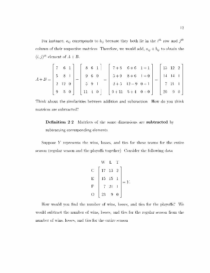
For instance, aij corresponds to bij because they both lie in the ith row and jth
column of their respective matrices. Therefore, we would add, aij + bij to obtain the
(i; j)th element of A+B:
A+B =
26666666664
7 6 1
5 8 1
2 12 0
9 5 0
37777777775+
26666666664
8 6 1
9 6 0
5 9 1
11 4 0
37777777775=
26666666664
7 + 8 6 + 6 1 + 1
5 + 9 8 + 6 1 + 0
2 + 5 12 + 9 0 + 1
9 + 11 5 + 4 0 + 0
37777777775=
26666666664
15 12 2
14 14 1
7 21 1
20 9 0
37777777775
Think about the similarities between addition and subtraction. How do you think
matrices are subtracted?
De�nition 2.2 Matrices of the same dimensions are subtracted by
subtracting corresponding elements.
Suppose Y represents the wins, losses, and ties for these teams for the entire
season (regular season and the playo�s together). Consider the following data
C
E
F
O
W L T26666666664
17 13 2
15 15 1
7 21 1
23 9 0
37777777775= Y:
How would you �nd the number of wins, losses, and ties for the playo�s? We
would subtract the number of wins, losses, and ties for the regular season from the
number of wins, losses, and ties for the entire season.

13
Y � (A+B) =
26666666664
17 13 2
15 15 1
7 21 1
23 9 0
37777777775�
26666666664
15 12 2
14 14 1
7 21 1
20 9 0
37777777775=
26666666664
17� 15 13� 12 2� 2
15� 14 15� 14 1� 1
7� 7 21� 21 1� 1
23� 20 9� 9 0� 0
37777777775
=
26666666664
2 1 0
1 1 0
0 0 0
3 0 0
37777777775
Remark 5 Remember, to add (or subtract) matrices, add (or subtract)
corresponding elements.
The addition property of zero for real numbers tells us that r+0 = 0+r = r. There
is also an addition property of zero for matrices which states that A+0 = 0+A = A
where 0 represents the zero matrix of the same dimensions as A.
De�nition 2.3 A zero matrix is a matrix which has the number 0 for
each of its elements.
Remark 6 We say \a" zero matrix instead of \the" zero matrix because
for di�erent pairs of dimensions, we have di�erent zero matrices. However,
for a given pair of dimensions, the zero matrix is unique because zero is
unique in the real number system. It is usual to merely say the zero matrix
and not refer to its dimensions when no confusion can arise.
Questions
1. So far, we have worked with speci�c examples. In general, does A+B = B+A?
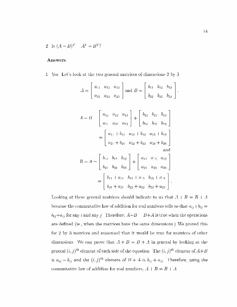
14
2. Is (A+B)T = AT +B
T ?
Answers
1. Yes. Let's look at the two general matrices of dimensions 2 by 3
A =
264 a11 a12 a13
a21 a22 a23
375 and B =
264 b11 b12 b13
b21 b22 b23
375 :
A +B =
264 a11 a12 a13
a21 a22 a23
375 +
264 b11 b12 b13
b21 b22 b23
375
=
264 a11 + b11 a12 + b12 a13 + b13
a21 + b21 a22 + b22 a23 + b23
375
and
B + A =
264 b11 b12 b13
b21 b22 b23
375+
264 a11 a12 a13
a21 a22 a23
375
=
264 b11 + a11 b12 + a12 b13 + a13
b21 + a21 b22 + a22 b23 + a23
375 :
Looking at these general matrices should indicate to us that A + B = B + A
because the commutative law of addition for real numbers tells us that aij+bij =
bij+aij for any i and any j. Therefore, A+B = B+A is true when the operations
are de�ned (ie., when the matrices have the same dimensions.) We proved this
for 2 by 3 matrices and reasonsed that it would be true for matrices of other
dimensions. We can prove that A + B = B + A in general by looking at the
general (i; j)th element of each side of the equation. The (i; j)th element of A+B
is aij + bij and the (i; j)th element of B + A is bij + aij. Therefore, using the
commutative law of addition for real numbers, A +B = B + A.
15
2. Yes, (A+B)T = AT +B
T: Let us look at a generic element from each side of the
equation. First, let's look at the left side of the equation. A generic element of
A+B would be aij+ bij: When this matrix is transposed, the generic element is
aji+ bji: Therefore, a generic element of the left side of the equation is aji+ bji,
which is exactly the same as a generic element of the right side of the equation.
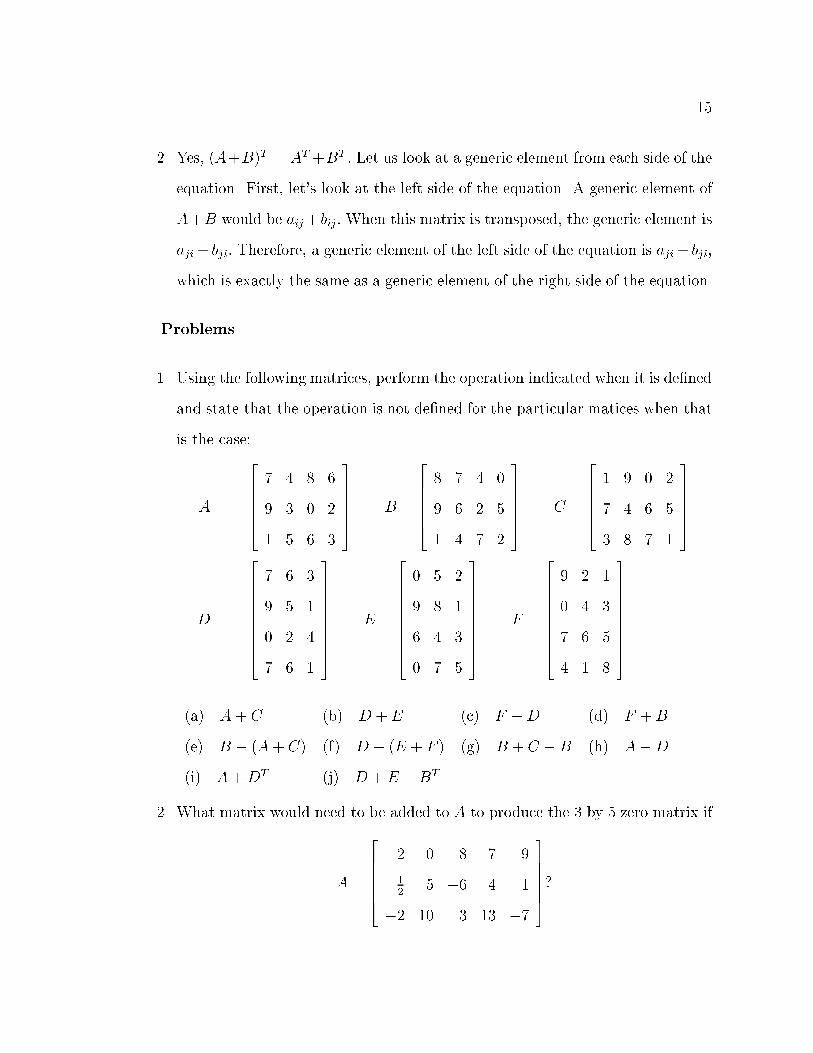
Problems
1. Using the following matrices, perform the operation indicated when it is de�ned
and state that the operation is not de�ned for the particular matices when that
is the case:
A =
2666664
7 4 8 6
9 3 0 2
1 5 6 3
3777775
B =
2666664
8 7 4 0
9 6 2 5
1 4 7 2
3777775
C =
2666664
1 9 0 2
7 4 6 5
3 8 7 1
3777775
D =
26666666664
7 6 3
9 5 1
0 2 4
7 6 1
37777777775
E =
26666666664
0 5 2
9 8 1
6 4 3
0 7 5
37777777775
F =
26666666664
9 2 1
0 4 3
7 6 5
4 1 8
37777777775
(a) A + C (b) D + E (c) F �D (d) F +B
(e) B � (A+ C) (f) D � (E + F ) (g) B + C � B (h) A�D
(i) A+DT (j) D + E �B
T
2. What matrix would need to be added to A to produce the 3 by 5 zero matrix if
A =
2666664
2 0 �8 7 �9
12
5 �6 4 1
�2 10 3 13 �7
3777775?

16
3. Matrix A represents the number of wins and losses for these teams in one year
and B represents the number of wins and losses for the next year.
Lions
Tigers
Bears
W L2666664
5 8
9 4
7 6
3777775= A
Lions
Tigers
Bears
W L2666664
7 5
6 6
4 8
3777775= B
(a) What are the teams' records for the two years combined?
(b) Write a sentence about what row 3 tells us.
(c) If the three season record for these teams is represented by C, how many
games did each team win and lose in the third year?
Lions
Tigers
Bears
W L2666664
20 19
22 17
16 23
3777775= C
4. Matrix A represents the points scored from three kinds of shots made by each
team during the �rst period of a basketball game, B represents the same in-
formation from the second period, C represents the same information from the
third period, and E represents the total number of points scored from each of
the three kinds of shots in the game by each team. The column for free throws
is labeled by FT, �eld goals by FG, and three-point shots by T.
(a) How many points of each kind were scored by each team in the fourth
period? (There are 4 periods in a basketball game).
Home
Visitor
FT FG T264 5 12 3
3 10 0
375 = A
Home
Visitor
FT FG T264 7 16 0
4 18 3
375 = B
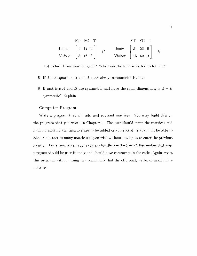
17
Home
Visitor
FT FG T264 3 12 3
3 16 3
375 = C
Home
Visitor
FT FG T264 21 58 6
15 60 9
375= E
(b) Which team won the game? What was the �nal score for each team?
5. If A is a square matrix, is A+ AT always symmetric? Explain.
6. If matrices A and B are symmetric and have the same dimensions, is A � B
symmetric? Explain.
Computer Program
Write a program that will add and subtract matrices. You may build this on
the program that you wrote in Chapter 1. The user should enter the matrices and
indicate whether the matrices are to be added or subtracted. You should be able to
add or subtract as many matrices as you wish without having to re-enter the previous
solution. For example, can your program handle A+B�C+D? Remember that your
program should be user-friendly and should have comments in the code. Again, write
this program without using any commands that directly read, write, or manipulate
matrices.

18
Chapter 3
Multiplication of Matrices
We have three recipes for breakfast foods. Each recipe feeds three people. The
ingredients are as follows:
Pancakes: 2 cups baking mix, 2 eggs, and 1 cup milk.
Biscuits: 214cups baking mix and 3
4cups milk.
Wa�es: 2 cups baking mix, 1 egg, 113cups milk, and 2 tablespoons vegetable oil.
Let's write this in the form of a labeled matrix so that it is easier to read.
P
B
W
Bm E M O2666664
2 2 1 0
214
0 34
0
2 1 113
2
3777775= R
If we want to feed 6 people instead of 3, what do we need to do? We double each
recipe. That means we need twice as much of each ingredient, so we multiply every
element of the matrix by the number 2.
2R = 2
2666664
2 2 1 0
214
0 34
0
2 1 113
2
3777775=
2666664
4 4 2 0
412
0 112
0
4 2 223
4
3777775
When we multiply a matrix by a real number, we call the real number a scalar and call
the operation scalar multiplication. Scalar multiplication consists of multiplying
each element of a matrix by a given scalar. We use the terms scalar and scalar
multiplication because, in abstract algebra, we often have the need to consider more
general scalars than real numbers. However, in this book, we restrict our attention
to scalars that are real numbers.
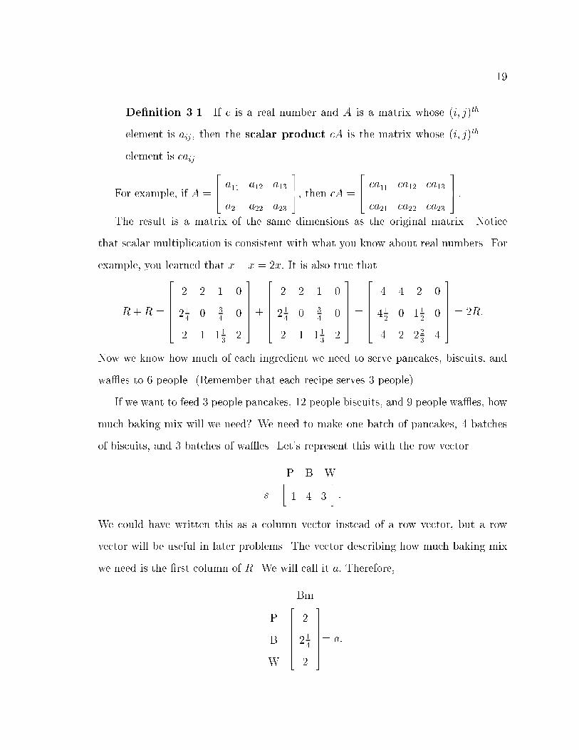
19
De�nition 3.1 If c is a real number and A is a matrix whose (i; j)th
element is aij, then the scalar product cA is the matrix whose (i; j)th
element is caij.
For example, if A =
264 a11 a12 a13
a21 a22 a23
375, then cA =
264 ca11 ca12 ca13
ca21 ca22 ca23
375 :
The result is a matrix of the same dimensions as the original matrix. Notice
that scalar multiplication is consistent with what you know about real numbers. For
example, you learned that x+ x = 2x: It is also true that
R +R =
2666664
2 2 1 0
214
0 34
0
2 1 113
2
3777775+
2666664
2 2 1 0
214
0 34
0
2 1 113
2
3777775=
2666664
4 4 2 0
412
0 112
0
4 2 223
4
3777775= 2R:
Now we know how much of each ingredient we need to serve pancakes, biscuits, and
wa�es to 6 people. (Remember that each recipe serves 3 people).
If we want to feed 3 people pancakes, 12 people biscuits, and 9 people wa�es, how
much baking mix will we need? We need to make one batch of pancakes, 4 batches
of biscuits, and 3 batches of wa�es. Let's represent this with the row vector
s =
P B W�1 4 3
�:
We could have written this as a column vector instead of a row vector, but a row
vector will be useful in later problems. The vector describing how much baking mix
we need is the �rst column of R. We will call it a: Therefore,
P
B
W
Bm2666664
2
214
2
3777775= a:

20
We need 1 � 2 + 4 � 214+ 2 � 3 = 17 cups of baking mix. The process by which we
found the number of cups of baking mix needed is called �nding the inner product
of two vectors.
De�nition 3.2 The inner product of n-vectors x and y, denoted by
hx; yi ; is x1y1+x2y2+ : : :+xnyn where n is the dimension of the vectors.
Notice that the de�nition of inner product requires the vectors to have the same
dimension. The inner product of two vectors is a scalar. Therefore, hs; ai = 17:
Remark 7 Some people refer to the inner product as the dot product
and denote it x � y:
What would we do if we wanted to know how much of each ingredient we need
for 1 batch of pancakes, 4 batches of biscuits, and 3 batches of wa�es? We would
take the inner product of s and a particular column of R to �nd out how much of
that particular ingredient we need. This procedure motivates our de�nition of matrix
multiplication which will be described in detail later in this chapter.
Now let's multiply our row vector, s, by our recipe matrix, R.
s =
P B W�1 4 3
� P
B
W
Bm E M O2666664
2 2 1 0
214
0 34
0
2 1 113
2
3777775= R
s �R =
�1 4 3
�2666664
2 2 1 0
214
0 34
0
2 1 113
2
3777775

21
hcolumn 1 of s;Ri = 1 � 2 + 4 � 214
+ 3 � 2 = 17
hcolumn 2 of s;Ri = 1 � 2 + 4 � 0 + 3 � 1 = 5
hcolumn 3 of s;Ri = 1 � 1 + 4 � 34
+ 3 � 113
= 8
hcolumn 4 of s;Ri = 1 � 0 + 4 � 0 + 3 � 2 = 6
s �R =
Bm E M O�17 5 8 6
�
We need 17 cups of baking mix, 5 eggs, 8 cups of milk, and 6 tablespoons of oil.
There are several interesting things to notice about matrix multiplication. We
multiplied a 1 by 3 matrix by a 3 by 4 matrix and got a 1 by 4 matrix. This pattern
will always hold when we multiply. The middle numbers must be the same (like the
threes were in this case), when we multiply matrices. The resulting matrix will always
have the dimensions of the outside numbers (1 by 4 in this case) when multiplication
is de�ned. The following picture expresses the requirements on the dimensions:
m n p q
agreemust
newdimensions
by by*
Even though the labels are not a formal part of the matrix, and are not always
attached to a matrix, this also happens with the labels. The labels of the inside
dimensions must agree if we want a meaningful product.
total by foods * foods by ingredients
agree
newlabels

22
The label, total by ingredients, is meaningful because foods was the label for the
inside dimensions of both matrices that we multiplied.
Let's also look closely at how we multiply the matrices because we will multiply
matrices with larger dimensions later. This is a hands on activity. Take your left
pointer �nger and place it at the beginning of the �rst row of the �rst matrix (the
only row we have in this case). Take your right pointer �nger and place it on the �rst
number of the �rst column of the second matrix. Multiply the two numbers to which
you are pointing. Each time you move, your left hand will go across the row, and your
right hand will go down the column. When you reach the end of the row and column,
add the numbers you have obtained from the multiplications. This number goes in
the �rst row and �rst column of your product matrix. This is the same as taking the
inner product of the �rst row of the �rst matrix and the �rst column of the second
matrix. Now you can move to the �rst row, second column doing the same thing.
This number will go in the �rst row, second column of your product matrix. In short,
position ij of your product matrix consists of the inner product of the ith row of your
�rst matrix and the jth column of the second matrix. This is a lot easier to do than it
is to describe! Your left hand will move across and your right hand will move down.
Do this for every row and column combination to get your product matrix. No, you
are not too old to do this. A lot of college students multiply matrices this way. After
you do this enough times, your hands will not let you do it incorrectly ever again.
This picture depicts the motions necessary to �nd a product:
Inner product of row i with column j equals position ij
23
De�nition 3.3 Consider the m by p matrix A and the p by n matrix
B. By the matrix product A times B, we mean the m by n matrix
whose (i; j)th element is the inner product of the ith row of A with the jth
column of B.
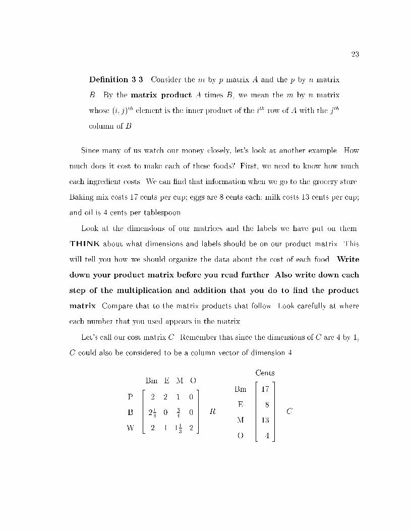
Since many of us watch our money closely, let's look at another example. How
much does it cost to make each of these foods? First, we need to know how much
each ingredient costs. We can �nd that information when we go to the grocery store.
Baking mix costs 17 cents per cup; eggs are 8 cents each; milk costs 13 cents per cup;
and oil is 4 cents per tablespoon.
Look at the dimensions of our matrices and the labels we have put on them.
THINK about what dimensions and labels should be on our product matrix. This
will tell you how we should organize the data about the cost of each food. Write
down your product matrix before you read further. Also write down each
step of the multiplication and addition that you do to �nd the product
matrix. Compare that to the matrix products that follow. Look carefully at where
each number that you used appears in the matrix.
Let's call our cost matrix C. Remember that since the dimensions of C are 4 by 1,
C could also be considered to be a column vector of dimension 4.
P
B
W
Bm E M O2666664
2 2 1 0
214
0 34
0
2 1 113
2
3777775= R
Bm
E
M
O
Cents26666666664
17
8
13
4
37777777775= C
24
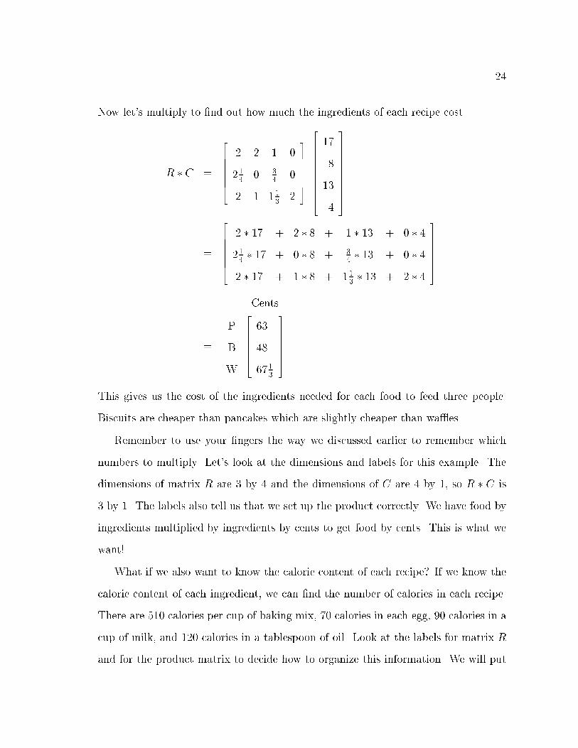
Now let's multiply to �nd out how much the ingredients of each recipe cost.
R � C =
2666664
2 2 1 0
214
0 34
0
2 1 113
2
3777775
26666666664
17
8
13
4
37777777775
=
2666664
2 � 17 + 2 � 8 + 1 � 13 + 0 � 4
214� 17 + 0 � 8 + 3
4� 13 + 0 � 4
2 � 17 + 1 � 8 + 113� 13 + 2 � 4
3777775
=
P
B
W
Cents2666664
63
48
6713
3777775
This gives us the cost of the ingredients needed for each food to feed three people.
Biscuits are cheaper than pancakes which are slightly cheaper than wa�es.
Remember to use your �ngers the way we discussed earlier to remember which
numbers to multiply. Let's look at the dimensions and labels for this example. The
dimensions of matrix R are 3 by 4 and the dimensions of C are 4 by 1, so R � C is
3 by 1. The labels also tell us that we set up the product correctly. We have food by
ingredients multiplied by ingredients by cents to get food by cents. This is what we
want!
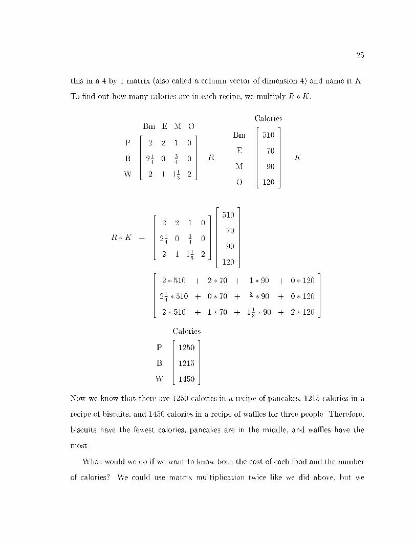
What if we also want to know the calorie content of each recipe? If we know the
calorie content of each ingredient, we can �nd the number of calories in each recipe.
There are 510 calories per cup of baking mix, 70 calories in each egg, 90 calories in a
cup of milk, and 120 calories in a tablespoon of oil. Look at the labels for matrix R
and for the product matrix to decide how to organize this information. We will put
25
this in a 4 by 1 matrix (also called a column vector of dimension 4) and name it K.
To �nd out how many calories are in each recipe, we multiply R �K:
P
B
W
Bm E M O2666664
2 2 1 0
214
0 34
0
2 1 113
2
3777775= R
Bm
E
M
O
Calories26666666664
510
70
90
120
37777777775= K
R �K =
2666664
2 2 1 0
214
0 34
0
2 1 113
2
3777775
26666666664
510
70
90
120
37777777775
=
2666664
2 � 510 + 2 � 70 + 1 � 90 + 0 � 120
214� 510 + 0 � 70 + 3
4� 90 + 0 � 120
2 � 510 + 1 � 70 + 113� 90 + 2 � 120
3777775
=
P
B
W
Calories2666664
1250
1215
1450
3777775
Now we know that there are 1250 calories in a recipe of pancakes, 1215 calories in a
recipe of biscuits, and 1450 calories in a recipe of wa�es for three people. Therefore,
biscuits have the fewest calories, pancakes are in the middle, and wa�es have the
most.
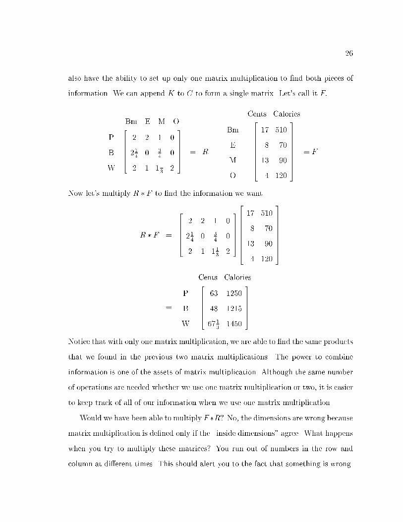
What would we do if we want to know both the cost of each food and the number
of calories? We could use matrix multiplication twice like we did above, but we
26
also have the ability to set up only one matrix multiplication to �nd both pieces of
information. We can append K to C to form a single matrix. Let's call it F:
P
B
W
Bm E M O2666664
2 2 1 0
214
0 34
0
2 1 113
2
3777775
= R
Bm
E
M
O
Cents Calories26666666664
17 510
8 70
13 90
4 120
37777777775
= F
Now let's multiply R � F to �nd the information we want.
R � F =
2666664
2 2 1 0
214
0 34
0
2 1 113
2
3777775
26666666664
17 510
8 70
13 90
4 120
37777777775
=
P
B
W
Cents Calories2666664
63 1250
48 1215
6713
1450
3777775
Notice that with only one matrix multiplication, we are able to �nd the same products
that we found in the previous two matrix multiplications. The power to combine
information is one of the assets of matrix multiplication. Although the same number
of operations are needed whether we use one matrix multiplication or two, it is easier
to keep track of all of our information when we use one matrix multiplication.
Would we have been able to multiply F �R? No, the dimensions are wrong because
matrix multiplication is de�ned only if the \inside dimensions" agree. What happens
when you try to multiply these matrices? You run out of numbers in the row and
column at di�erent times. This should alert you to the fact that something is wrong.
27
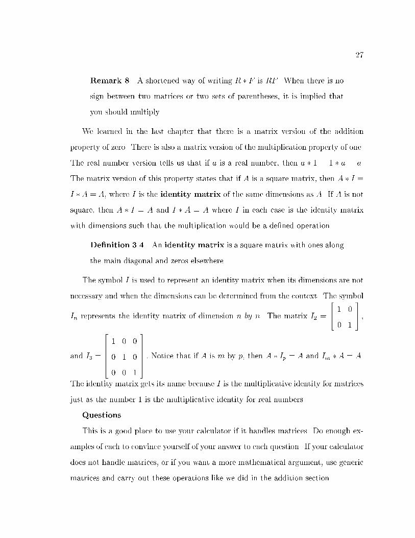
Remark 8 A shortened way of writing R � F is RF . When there is no
sign between two matrices or two sets of parentheses, it is implied that
you should multiply.
We learned in the last chapter that there is a matrix version of the addition
property of zero. There is also a matrix version of the multiplication property of one.
The real number version tells us that if a is a real number, then a � 1 = 1 � a = a.
The matrix version of this property states that if A is a square matrix, then A � I =
I �A = A, where I is the identity matrix of the same dimensions as A. If A is not
square, then A � I = A and I � A = A where I in each case is the identity matrix
with dimensions such that the multiplication would be a de�ned operation.
De�nition 3.4 An identity matrix is a square matrix with ones along
the main diagonal and zeros elsewhere.
The symbol I is used to represent an identity matrix when its dimensions are not
necessary and when the dimensions can be determined from the context. The symbol
In represents the identity matrix of dimension n by n. The matrix I2 =
264 1 0
0 1
375 ;
and I3 =
2666664
1 0 0
0 1 0
0 0 1
3777775: Notice that if A is m by p, then A � Ip = A and Im � A = A.
The identity matrix gets its name because I is the multiplicative identity for matrices
just as the number 1 is the multiplicative identity for real numbers.
Questions
This is a good place to use your calculator if it handles matrices. Do enough ex-
amples of each to convince yourself of your answer to each question. If your calculator
does not handle matrices, or if you want a more mathematical argument, use generic
matrices and carry out these operations like we did in the addition section.

28
Answer these questions on your own before you read beyond this para-
graph. Remember to consider the dimensions of the matrices.
1. Consider A =
264 a 0
0 a
375. Does AB = BA for all B for which matrix multiplica-
tion is de�ned?
2. In general, does AB = BA?
3. Does A(BC) = (AB)C?
4. Does A(B + C) = AB + AC?
5. Does (AB)T = BTAT ?
6. Does A� B = �(B � A)?
7. For real numbers, if ab = 0, we know that either a or b must be zero. Is it true
that AB = 0 implies that A or B is a zero matrix?
8. Are ATA and AA
T always symmetric?
Answers
1. Yes. Let's consider the generic 2 by 2 matrix B =
264 b11 b12
b21 b22
375. Let's look at
the left side of the equation; AB =
264 ab11 ab12
ab21 ab22
375. Now let's look at the right
side of the equation; BA =
264 b11a b12a
b21a b22a
375. Since a and each element of B are
scalars, the order of multiplication does not matter. Therefore, if A =
264 a 0
0 a
375,
then AB = BA for any B for which matrix multiplication is de�ned.
29
For the general case, A = aI, let's look at the left side of the equation. The
product AB = aIB = aB for any matrix B for which matrix multiplication is
de�ned. Therefore, a general element of this matrix is abij. Now, let's look at
the right side of the equation. We need to remember that a = aT because a is
a scalar. The product BA = BaI = Ba = (aTBT )T = (aBT )T . Each element
of the matrix aBT is abji, so the transpose of this matrix has elements abij.
Therefore, the two sides are equal.
2. No. Unlike multiplication with real numbers, AB 6= BA in general. There are
occasions when AB = BA, but these occasions are very rare. In fact, the only
time that AB = BA for every B is when A is a scalar multiple of the identity
matrix. It is very important to remember that AB is NOT, in general,
equal to BA.
3. If the dimensions are correct for multiplication, A(BC) = (AB)C. We call this
the associative property of matrices. An example with correct dimensions is
matrix A is 4 by 3, matrix B is 3 by 2, and matrix C is 2 by 5. This product
results in a 4 by 5 matrix. The associative property of matrices becomes quite
useful when you want to reduce the number of multiplications performed. Refer
to problem 5 for an example. The number of multiplications performed becomes
very important when you are dealing with large matrices.
4. Yes, A(B + C) = AB + AC. This means that the distributive property holds
for matrices.
5. Yes, (AB)T = BTAT: If matrix A is 4 by 3 and matrix B is 3 by 5, AB is 4 by 5,
so (AB)T is 5 by 4. Just by looking at dimensions, we can tell that (AB)T 6=
ATBT , because the dimensions of AT
BT tell us that this multiplication cannot
30
be performed. The dimensions of BTAT are correct for matrix multiplication
and give a resulting matrix that is 5 by 4. This is not a proof that (AB)T =
BTAT is true, but it is a good indication. Work several examples to convince
yourself that (AB)T = BTAT:
6. Yes, A � B = �(B � A) if the dimensions of A and B are the same so that
subtraction is de�ned. This is true because �(B�A) = �1(B�A) = �B+A =
A�B:
7. No. For example, if A =
264 1 2
3 6
375 and B =
264 �2 4
1 �2
375 ; then AB =
264 0 0
0 0
375 ;
but neither A nor B is a zero matrix. Remember that AB = 0 does NOT
imply that either A = 0 or B = 0:
8. Yes, ATA and AA
T are always symmetric. Remember that (AB)T = BTAT
and that a matrix is symmetric if it is equal to its transpose. Let's look at the
transpose of ATA; (AT
A)T = AT (AT )
T= A
TA. Therefore, AT
A is symmetric.
The same procedure proves that AAT is symmetric; (AAT )T = (AT )TAT =
AAT .
Problems
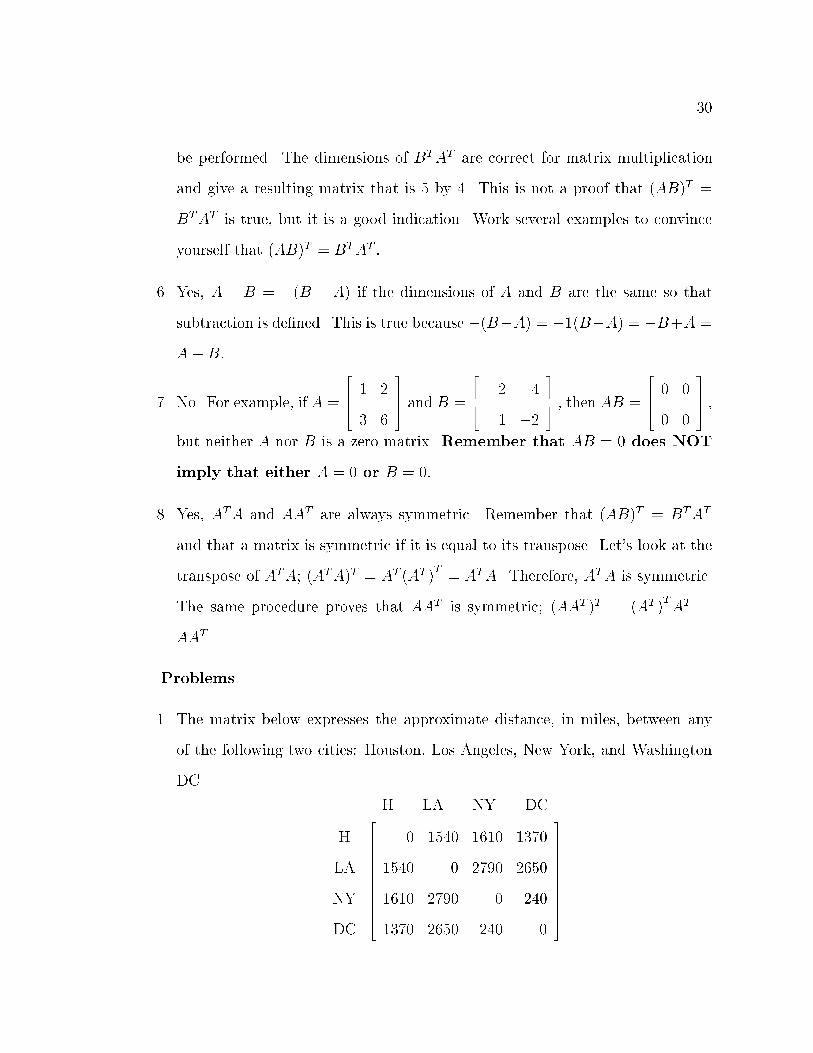
1. The matrix below expresses the approximate distance, in miles, between any
of the following two cities: Houston, Los Angeles, New York, and Washington
DC.
H
LA
NY
DC
H LA NY DC26666666664
0 1540 1610 1370
1540 0 2790 2650
1610 2790 0 240
1370 2650 240 0
37777777775

31
(a) What special kind of matrix is this (other than square and 4 by 4)?
(b) If we want to know the same information in kilometers, what should we
do? Remember, for our purposes here, one mile is equal to 1.6 kilometers.
(c) What is the resulting matrix when you perform the operation that you
suggested in part (b)?
2. Perform the operations requested below if they are possible using these matrices.
A =
2666664
5 9 2
1 7 6
3 4 8
3777775
B =
2666664
9 1 6
7 2 4
8 10 3
3777775
C =
�5 3 6
�D =
2666664
4
8
1
3777775
(a) 4C (b) AD (c) DA (d) BC (e) 3CB
(f) C(A +B) (g) AB (h) BA (i) CAD (j) DBC
(k) AD + (CB)T (l) DC (m) CD
3. The matrix G represents the average score for each student on tests, quizzes,
and homework. Tests are 50% of the grade, quizzes are 30% and homework is
20%.
Amy
Bill
Chou
David
Erica
T Q H266666666666664
78 80 75
76 90 95
72 70 85
60 70 80
84 80 90
377777777777775
= G
(a) Write the vector P expressing the percentages that would be used to �nd
the �nal grade for each student.
(b) Would GP or PG produce a matrix of the �nal grades?

32
(c) Using matrices, determine the �nal grade for each student. Please show
your work.
4. Does c (Ax) = A (cx) where c is a scalar, A is a 2 by 2 matrix, and x is a
dimension 2 column vector? Explain your answer.
5. Place the parentheses where needed to minimize the number of multiplications
performed to work this problem. How many simple multiplications did it take
to �nd T ?
T =
2666664
a
b
c
3777775�d e f
�2666664
g
h
k
3777775�l p q
�
6. Does A =
264 4 3
2 5
375 satisfy the equation 3A2
� 2A =
264 58 75
50 83
375? Explain why
A does or does not satisfy the equation. Note: For real numbers, a multiplied
by itself n times can be written as an. Similarly, the matrix A multiplied by
itself n times can be written as An. Therefore, A2 means AA:
Computer Program
Make changes and additions to your program from Chapter 2 so that it can also
multiply matrices. A warning message should be displayed if the matrices are not of
correct dimensions for the operation requested. Your program should be able to han-
dle (AB�C+D)E and other similar problems. Remember that your program should
be user-friendly and should have comments in the code. Again, write this program
without using any commands that directly read, write, or manipulate matrices.

33
Chapter 4
Equations
Solving equations is an important part of mathematics. If we are working with more
than one unknown at a time, we need to solve systems of equations. You may already
know how to solve a system of linear equations, but matrices provide a more compact
way to arrive at the solution. Matrices are also easier to manipulate on a computer
or calculator. Both of these facts will become more important when you work with
larger systems.
Let's look at a system of linear equations. The system
5x1 + 3x2 = 93
�4x1 � 2x2 = �66
can be written in matrix form as AX = B where
A =
264 5 3
�4 �2
375 ; X =
264 x1
x2
375 ; and B =
264 93
�66
375 :
However, you will usually see Ax = b rather than AX = B because most authors use
small letters to represent vectors. You can multiply this out to convince yourself that
AX = B does represent this system.
When you learned to solve systems of linear equations, you learned that
(a) you arrive at the same solution no matter which equation you write �rst;
(b) the solution doesn't change if you multiply an equation by a scalar other than
zero; and
(c) you can replace an equation with the sum of that equation and another equation
without changing the solution.
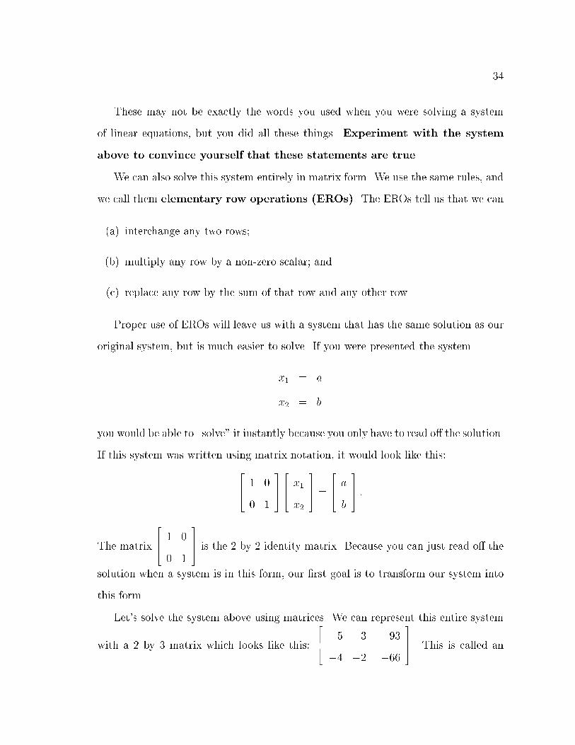
34
These may not be exactly the words you used when you were solving a system
of linear equations, but you did all these things. Experiment with the system
above to convince yourself that these statements are true.
We can also solve this system entirely in matrix form. We use the same rules, and
we call them elementary row operations (EROs). The EROs tell us that we can
(a) interchange any two rows;
(b) multiply any row by a non-zero scalar; and
(c) replace any row by the sum of that row and any other row.
Proper use of EROs will leave us with a system that has the same solution as our
original system, but is much easier to solve. If you were presented the system
x1 = a
x2 = b
you would be able to \solve" it instantly because you only have to read o� the solution.
If this system was written using matrix notation, it would look like this:
264 1 0
0 1
375264 x1
x2
375 =
264 a
b
375 :
The matrix
264 1 0
0 1
375 is the 2 by 2 identity matrix. Because you can just read o� the
solution when a system is in this form, our �rst goal is to transform our system into
this form.
Let's solve the system above using matrices. We can represent this entire system
with a 2 by 3 matrix which looks like this:
264 5 3
�4 �2
�������93
�66
375. This is called an
35
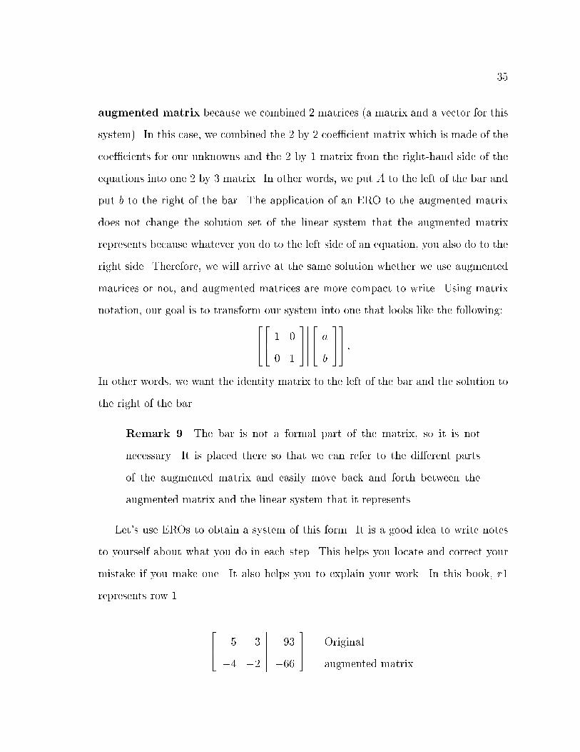
augmented matrix because we combined 2 matrices (a matrix and a vector for this
system). In this case, we combined the 2 by 2 coe�cient matrix which is made of the
coe�cients for our unknowns and the 2 by 1 matrix from the right-hand side of the
equations into one 2 by 3 matrix. In other words, we put A to the left of the bar and
put b to the right of the bar. The application of an ERO to the augmented matrix
does not change the solution set of the linear system that the augmented matrix
represents because whatever you do to the left side of an equation, you also do to the
right side. Therefore, we will arrive at the same solution whether we use augmented
matrices or not, and augmented matrices are more compact to write. Using matrix
notation, our goal is to transform our system into one that looks like the following:264264 1 0
0 1
375�������
264 a
b
375375 :
In other words, we want the identity matrix to the left of the bar and the solution to
the right of the bar.
Remark 9 The bar is not a formal part of the matrix, so it is not
necessary. It is placed there so that we can refer to the di�erent parts
of the augmented matrix and easily move back and forth between the
augmented matrix and the linear system that it represents.
Let's use EROs to obtain a system of this form. It is a good idea to write notes
to yourself about what you do in each step. This helps you locate and correct your
mistake if you make one. It also helps you to explain your work. In this book, r1
represents row 1.
264 5 3
�4 �2
�������93
�66
375 Original
augmented matrix

36
264 1 0:6
�4 �2
�������18:6
�66
375 r1� 5
264 1 0:6
0 0:4
�������18:6
8:4
375
4 � r1 + r2264 1 0:6
0 1
�������18:6
21
375
r2� 0:4264 1 0
0 1
�������6
21
375 �6 � r2 + r1
When we convert this from augmented matrix notation back to the algebraic notation
for a system of equations, it looks like this:
1x1 + 0x2 = 6
0x1 + 1x2 = 21
This tells us that x1 = 6 and x2 = 21. Substitute this solution into the sys-
tem to assure yourself that we are correct. If we systematically use elementary
row operations to obtain the identity matrix to the left of the bar, we call this the
Gauss-Jordan elimination method.
Now, let's solve the system
5x1 + 3x2 = 70
�4x1 � 2x2 = �56
using Gauss-Jordan elimination.
264 5 3
�4 �2
�������70
�56
375 Original
augmented matrix264 1 0:6
�4 �2
�������14
�56
375 r1� 5

37
264 1 0:6
0 0:4
�������14
0
375
4 � r1 + r2264 1 0:6
0 1
�������14
0
375
r2� 0:4264 1 0
0 1
�������14
0
375 �0:6 � r2 + r1
Look back at the two systems of equations that we solved. How are they similar? We
performed the same steps both times because the steps involved in solving a system
of equations depend only on the matrix that is to the left of the bar. If we want to
solve a system of equations with the same matrix A for di�erent b vectors that we
will be given at a later time, it would be nice if we did not have to do Gauss-Jordan
elimination every time.
Let's look at the scalar version of this equation, ax = b; to help us �nd a general
method for matrices. We know that x = a�1b if a 6= 0 because a�1 = 1=a where a�1
is called the multiplicative inverse or the reciprocal. There is something analogous to
this with matrices. It is also called the inverse. With scalars, a�1a = aa
�1 = 1.
De�nition 4.1 The matrix A�1 (called A inverse) is the inverse of a
square matrixA if A�1A = AA
�1 = I where I is the identity matrix.
Once we �nd A�1; Ax = b can be solved by matrix multiplication rather than
Gauss-Jordan elimination. We follow the algebraic steps below to �nd an expression
for x:
Ax = b
A�1Ax = A
�1b
Ix = A�1b

38
x = A�1b
This means that if we �nd A�1; we only need to multiply to solve systems with the
same matrix A for di�erent b vectors. Please remember that A�1b 6= bA
�1, so you
must multiply in the correct order.
Remark 10 If we have all the b vectors at the time when we wish to
solve the system, we can simply augment all the b vectors together on
the right side of the bar. Then the solution for each b vector will fall in
the column that originally contained that b vector. For example, if we
wished to solve Ax = b and Ax = c for the same A matrix, we could use
the augmented matrix
264 a1 a2
a3 a4
�������b1 c1
b2 c2
375 : When the matrix to the left
of the bar reaches the identity matrix by use of EROs, the solution to
Ax = b will be in the �rst column to the right of the bar, and the solution
to Ax = c will be in the second column to the right of the bar. Now you
may wonder why we would ever need an inverse. If we do not have all the
right-hand sides at the time when we solve the problem, we would �nd
A�1 and multiply as indicated earlier. This situation often occurs when
the solution to one system is the right-hand side of the next system.
Let's �nd A�1 for the same matrix that we have been using, A =
264 5 3
�4 �2
375.
We can do this by solving the equation AX = I for the n by n matrix X. Because
we know that AA�1 = I, we know that our solution, X; is the same as A�1:2
64 5 3
�4 �2
�������1 0
0 1
375 Original
augmented matrix264 1 0:6
�4 �2
�������0:2 0
0 1
375 r1� 5

39
264 1 0:6
0 0:4
�������0:2 0
0:8 1
375
4 � r1 + r2264 1 0:6
0 1
�������0:2 0
2 2:5
375
r2� 0:4264 1 0
0 1
��������1 �1:5
2 2:5
375 �0:6 � r2 + r1
Notice that we used the exact same steps again. We now know that A�1 =264 �1 �1:5
2 2:5
375 :
Remark 11 In computational mathematics, the inverse is very seldom
found because other methods exist that serve the same purpose and re-
quire fewer steps. However, the inverse will serve our needs at this level
and is important in the theory of matrices.
Using the Gauss-Jordan eliminationmethod, let's �nd A�1 where A =
2666664
0 2 4
4 2 3
1 3 6
3777775.
2666664
0 2 4
4 2 3
1 3 6
�����������
1 0 0
0 1 0
0 0 1
3777775
Original
augmented
matrix2666664
1 3 6
4 2 3
0 2 4
�����������
0 0 1
0 1 0
1 0 0
3777775
Switch r1 and r3 because we cannot
have a zero on the main diagonal, and
we would prefer 1 rather than 4.2666664
1 3 6
0 �10 �21
0 2 4
�����������
0 0 1
0 1 �4
1 0 0
3777775 �4 � r1 + r2
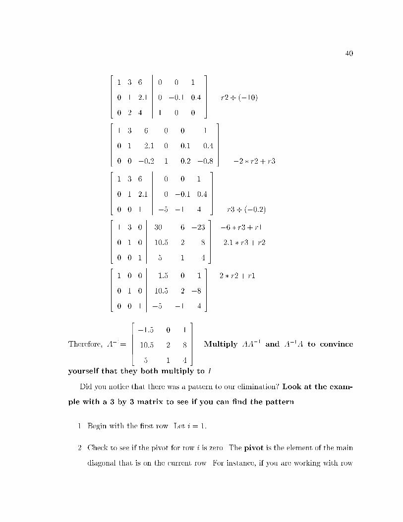
40
2666664
1 3 6
0 1 2:1
0 2 4
�����������
0 0 1
0 �0:1 0:4
1 0 0
3777775 r2� (�10)
2666664
1 3 6
0 1 2:1
0 0 �0:2
�����������
0 0 1
0 �0:1 0:4
1 0:2 �0:8
3777775
�2 � r2 + r32666664
1 3 6
0 1 2:1
0 0 1
�����������
0 0 1
0 �0:1 0:4
�5 �1 4
3777775
r3� (�0:2)2666664
1 3 0
0 1 0
0 0 1
�����������
30 6 �23
10:5 2 �8
�5 �1 4
3777775
�6 � r3 + r1
�2:1 � r3 + r2
2666664
1 0 0
0 1 0
0 0 1
�����������
�1:5 0 1
10:5 2 �8
�5 �1 4
3777775
�2 � r2 + r1
Therefore, A�1=
2666664
�1:5 0 1
10:5 2 �8
�5 �1 4
3777775. Multiply AA
�1and A
�1A to convince
yourself that they both multiply to I.
Did you notice that there was a pattern to our elimination? Look at the exam-
ple with a 3 by 3 matrix to see if you can �nd the pattern.
1. Begin with the �rst row. Let i = 1:
2. Check to see if the pivot for row i is zero. The pivot is the element of the main
diagonal that is on the current row. For instance, if you are working with row

41
i, then the pivot element is aii. If the pivot is zero, exchange that row with a
row below it that does not contain a zero in column i. If this is not possible,
then an inverse to that matrix does not exist.
3. Divide every element of row i by the pivot.
4. For every row below row i, replace that row with the sum of that row and a
multiple of row i so that each new element in column i below row i is zero.
5. Let i = i + 1: This means that you move to the next row and column. Repeat
steps 2 through 5 until you have zeros for every element below the main diagonal.
Now you have a matrix to the left of the bar that is called upper triangular
because all the non-zero numbers fall in the triangle above and including the
main diagonal.
6. Now we work to get zeros above the main diagonal. The index i should be equal
to the number of rows.
7. For every row above row i, replace that row with the sum of that row and a
multiple of row i so that each new element in column i above row i is zero. You
will notice that the zeros below the main diagonal are still zeros.
8. Let i = i � 1: This means that you move to the left one column and up a
row. Repeat steps 6-8 until you have zeros for every element above the main
diagonal. Since the zeros below the main diagonal did not change, you now have
a diagonal matrix to the left of the bar because all the non-zero elements lie
on the main diagonal. Since all the elements along the diagonal of this diagonal
matrix are the number one, this matrix is the identity matrix. Therefore, the
matrix to the right of the bar is our solution.
42
Remark 12 Notice that we obtain all the zeros below the main diagonal
before we work to get any zeros above the main diagonal. Other books
tell you to obtain all the zeros needed for a column above and below the
diagonal before you move to the next column. That method makes the
problem easier to code on a computer, but the method that we used often
requires fewer calculations.
WARNING: We know that a�1 is not de�ned when a = 0: It is also true that
A�1 is not always de�ned. Is it possible to �nd a unique solution to the system if the
matrix A does not have an inverse? No it is not. You will learn more about this in
Chapter 6.
We know that we can use the Gauss-Jordan elimination method to solve a system
of equations using matrices, but we don't really have to do all that work if we are
only trying to solve a system of linear equations. It is true that it is easy to solve a
system if the identity matrix is to the left of the bar because you can just read o�
the answer. However, it is also fairly easy if the matrix to the left of the bar is upper
triangular because you can read the last element of the solution and substitute it into
the previous equation to obtain another element. Repeated use of substitution will
yield the entire solution. Therefore there is a method called Gaussian elimination
that stops row operations after you have an upper triangular matrix to the left of the
bar. At that point, you use back-substitution to �nd the remaining values of the
solution. This is very similar to the way you learned to solve systems of equations
algebraically. Once you �nd a solution, you substitute it in everywhere to decrease
the size of your system. Let's go back to our original 2 by 2 matrix example in this
section. 264 5 3
�4 �2
�������93
�66
375 Original
augmented matrix

43
264 1 0:6
�4 �2
�������18:6
�66
375 r1� 5
264 1 0:6
0 0:4
�������18:6
8:4
375
4 � r1 + r2264 1 0:6
0 1
�������18:6
21
375
r2� 0:4
In Gaussian elimination, we can stop performing row operations now since we have an
upper triangular matrix to the left of the bar. When we translate from the augmented
matrix into a system of equations, we get
x1 + 0:6x2 = 18:6
x2 = 21:
We can read from the second equation that x2 = 21. We substitute 21 for x2 into
the �rst equation to get x1 + 0:6(21) = 18:6, so x1 = 6. This is the same solution as
before, and Gaussian elimination requires fewer operations than does Gauss-Jordan
elimination. Try this with the 3 by 3 matrix to see that you get the same
solution. You can see for a 3 by 3 or larger matrix that fewer steps are required.
In fact, Gaussian elimination requires approximately n3=3 steps and Gauss-Jordan
elimination requires approximately n3=2 steps. You can read more about this in the
last chapter of this book.
4.1 Coding
Did you ever make up codes so that you could pass secret notes to your friends? See
if you can �gure out this coded phrase: 69 108 130 159 -50 -86 -96 -124 . Don't
worry if you don't know it now; by the end of this chapter, you will be able to �gure
out the word. What sort of codes did you use? A very popular code is to give each

44
letter of the alphabet a number.
A=1 J=10 S=19
B=2 K=11 T=20
C=3 L=12 U=21
D=4 M=13 V=22
E=5 N=14 W=23
F=6 O=15 X=24
G=7 P=16 Y=25
H=8 Q=17 Z=26
I=9 R=18 space=27
Unfortunately, this code is so well-known, that your message would not be very se-
cretive. Some people choose to shift the code above so that A=10, B=11,: : :, R=1,: : :,
Z=9 or something similar. However, since each letter is represented by a particular
number and that number always stands for the same letter, this type of code is also
easily broken. We need a code that is more di�cult to break but is still easy to encode
and decode. Let's look at one way to do this.
In order to send a secret message, you and your friend need to pick a matrix
that has an inverse to be your secret coding matrix. For this example, let's use
A =
264 1 2
3 4
375. Therefore, A�1 =
264 �2 1
1:5 �0:5
375.
Now we need to pick a message to send. Let's send the word \Smiles". We will
derive our secret code by multiplying AB where B is our message. Since A has
two columns, B must have two rows (in order for matrix multiplications to work).
Therefore, B must be a 2 by 3 matrix
B =
264 S M I
L E S
375 :

45
Notice that we chose to write our message across the rows. We need to let our friend
know this when we choose the secret coding matrix because we could have just as
easily written our letters down the columms. Since we want this message to be coded,
we need to pick up numbers for each letter. We will stick with the standard A=1,
B=2, etc. Therefore,
B =
264 19 13 9
12 5 19
375 :
To code our message, we need to multiply AB. So
AB =
264 1 2
3 4
375264 19 13 19
12 5 19
375 =
264 43 23 47
105 59 103
375 :
Since we want to add one more layer of secrecy to our code, we will write out the
code in a line so that we don't give our \enemy" a clue that we used matrices to code
and that our coding matrix had 2 rows. Now we can broadcast 43 23 47 105 59 103 in
a public place if we want, and our message will be safe. When our friend receives our
messages 43 23 47 105 59 103, she will want to decode it. She knows that our coding
matrix was A =
264 1 2
3 4
375, and she knows our method of coding (writing across the
rows, AB = our code, and A=1, B=2, etc.) Since our coding matrix has two rows,
our code, C, must also have twor rows. Therefore, she can convert our message back
into the matrix
C =
264 43 23 47
105 59 103
375 :
To solve AB = C, she multiplies on the left by A�1 to get B = A�1C. Therefore,
B =
264 �2 1
1:5 �0:5
375264 43 23 47
105 59 103
375 =
264 19 13 9
12 5 19
375 :

46
She can convert this back into the matrix
264 S M I
L E S
375 to get SMILES. If we use
the same coding matrix to code the work SMIRK, we get
C =
264 1 2
3 4
375264 19 13 9
18 11 27
375 =
264 55 35 63
129 83 135
375 :
If we look at all three words we have coded with this same coding matrix, we see
SMILES 43 23 47 105 59 103
SMIRK 55 35 63 129 83 135
MILE 37 19 87 47
Notice that although these words share many letters, their codes are not similar
at all. Also notice that the number 47 represents the letter I in SMILES and the
letter E in MILE. These are some of the features that make this sort of code so
di�cult to break. Even if our \enemy" knew that we we were coding using matrices,
he would not know what size coding matrix we used or which numbers were in that
coding matrix. Since the numbers in the coding matrix can be any real numbers (even
negative numbers and fractions0, it would take a LONG time to guess the correct
matrix even with the help of a very fast computer.
The matrix
A =
2666664
0 2 4
4 2 3
1 3 6
3777775
was used to code the message 42 62 96 53 63 166 68 97 165. So to decode the
message, we need to �nd A�1. Since we computed it earlier in the chapter, we know
that
A�1 =
2666664
�1:5 0 1
10:5 2 �8
�5 �1 4
3777775:

47
Because we coded using a 3 by 3 matrix, we need to break our message into 3 rows.
Therefore, our message should be written as
B =
2666664
42 62 96
53 63 166
68 97 165
3777775:
When we multiply A�1, we get
2666664
�1:5 0 1
10:5 2 8
�5 �1 4
3777775
2666664
42 62 96
53 63 166
68 97 165
3777775=
2666664
5 4 21
3 1 20
9 15 4
3777775
which translates into the word \education." Now can you decode the message from
the beginning of this section? It was encoded using the same format as the other and
we used the coding matrix
A =
264 5 3
�4 �2
375 :
Coding is a fun way to use matrices and their inverses, but it also has impor-
tant practical applications when governments andother organizations try to transmit
private messages over public systems such as a radio or satellite.
Questions
1. There is a formula that can be used to �nd the inverse of a 2 by 2 matrix. Look
at A and A�1 for several 2 by 2 matrices or perform Gauss-Jordan elimination on
an augmented matrix formed from a general 2 by 2 matrix to �nd this formula.
2. Does a non-square matrix have an inverse?
3. An upper triangular matrix was described in the chapter. Describe and give an
example of a lower triangular matrix.

48
4. Is (A�1)T = (AT )�1?
Extension Questions
5. Is x = A�1L b always a solution to Ax = b? You will probably need to read the
answer to the second question before answering this one.
6. Is x = A�1L b the only solution to Ax = b when there is a solution?
Answers
1. If A =
264 a b
c d
375
264 a b
c d
�������1 0
0 1
375 Original
augmented matrix264 1 b
a
c d
�������1a
0
0 1
375 r1� a
264 1 b
a
0 ad�bc
a
�������1a
0
�c
a1
375
�c � r1 + r2264 1 b
a
0 1
�������1a
0
�cad�bc
aad�bc
375
r2� ad�bca2
64 1 0
0 1
�������d
ad�bc�b
ad�bc
�c
ad�bc
a
ad�bc
375
�ba� r2 + r1
This can also be written as A�1 = 1ad�bc
264 d �b
�c a
375 : This formula for the
inverse of a 2 by 2 matrix is a good one to memorize.
2. No. Only square matrices can have an inverse such that A�1A = AA
�1 = I.
However, there are one-sided inverses for some rectangular matrices, A, such

49
that A�1L A = I or AA�1
R = I. For example, if A =
264 1 2 1
2 5 1
375 and B =
2666664
2 �2
�1 1
1 0
3777775; then AB =
264 1 0
0 1
375 and BA =
2666664
�2 �6 0
1 3 0
1 2 1
3777775: This means
that B is a right inverse for A. It is a \right" inverse because A multiplied by
B on the right produces an identity matrix. It is \an" inverse rather than \the"
inverse because it is not unique. The matrix
C =
2666664
2 �5
�1 2
1 1
3777775
is also a right inverse of A: A left inverse can be represented by A�1L and a right
inverse can be represented by A�1R :
Remark 13 If someone asks if matrix A has an inverse, he or she
is referring to a matrix A�1 such that A�1A = AA
�1 = I. Therefore,
unless the matrix A is square, just AB = I or BA = I is not su�cient
proof that B is the inverse of A; it is only proof that B is at least a
one-sided inverse of A: However, if the matrix is square and BA = I
or AB = I, then B = A�1and A
�1A = AA
�1 = I. You can �nd a
proof of this in a college linear algebra text.
3. A lower triangular matrix has all the non-zero numbers on and below the main
diagonal. All the numbers above the main diagonal are zero. An example is
A =
2666664
5 0 0
2 3 0
1 0 6
3777775:
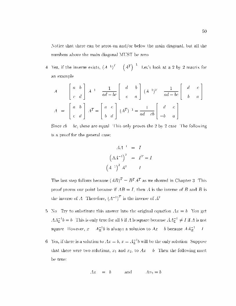
50
Notice that there can be zeros on and/or below the main diagonal, but all the
numbers above the main diagonal MUST be zero.
4. Yes, if the inverse exists, (A�1)T=�AT��1. Let's look at a 2 by 2 matrix for
an example.
A =
264 a b
c d
375 A
�1 =1
ad� bc
264 d �b
�c a
375 (A�1)T =
1
ad� bc
264 d �c
�b a
375
A =
264 a b
c d
375 A
T =
264 a c
b d
375 (AT )�1 =
1
ad� cb
264 d �c
�b a
375
Since cb = bc, these are equal. This only proves the 2 by 2 case. The following
is a proof for the general case:
AA�1 = I
�AA
�1�T
= IT = I
�A�1�T
AT = I
The last step follows because (AB)T= B
TAT as we showed in Chapter 3. This
proof proves our point because if AB = I, then A is the inverse of B and B is
the inverse of A. Therefore, (A�1)Tis the inverse of AT .
5. No. Try to substitute this answer into the original equation Ax = b. You get
AA�1L b = b. This is only true for all b if A is square because AA�1
L 6= I if A is not
square. However, x = A�1R b is always a solution to Ax = b because AA�1
R = I.
6. Yes, if there is a solution to Ax = b, x = A�1L b will be the only solution. Suppose
that there were two solutions, x1 and x2, to Ax = b. Then the following must
be true:
Ax1 = b and Ax2 = b

51
A�1L Ax1 = A
�1L b and A
�1L Ax2 = A
�1L b
x1 = A�1L b and x2 = A
�1L b
Therefore, x1 = x2. This follows directly from our original assumption, but
contradicts it. This means that our original assumption must be wrong. This
is an example of proof by contradiction.
Problems
1. If you know that Ax = b where A is a matrix and x and b are vectors, can you
say for sure that x = A�1b? Why or why not?
2. If A�1 exists, what is (AA�1)(A�1A)T ?
3. Use elementary row operations on augmented matrices to solve these systems
of equations for x. Use Gauss-Jordan elimination for (a) and (c). Use Gaussian
elimination and back-substitution for (b) and (d).
(a) 3x1 + 5x2 = 2 and 2x1 + 4x2 = 1
(b) 2x1 + 9x2 = �3 and x1 + 3x2 = 6
(c) Ax = b where A =
2666664
1 2 1
2 6 3
3 8 5
3777775and b =
2666664
2
3
4
3777775
(d) Ax = b where A =
2666664
2 3 1
1 3 3
3 3 1
3777775and b =
2666664
3
12
6
3777775
4. Find the inverses of these matrices:
(a) A =
264 5 3
5 4
375
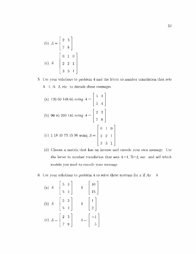
52
(b) A =
264 2 3
7 8
375
(c) A =
2666664
0 1 0
2 2 1
3 3 1
3777775
5. Use your solutions to problem 4 and the letter to number translation that sets
A=1, B=2, etc. to decode these messages.
(a) 126 60 148 65 using A =
264 5 3
5 4
375
(b) 90 45 260 145 using A =
264 2 3
7 8
375
(c) 1 18 40 73 53 96 using A =
2666664
0 1 0
2 2 1
3 3 1
3777775
(d) Choose a matrix that has an inverse and encode your own message. Use
the letter to number translation that sets A=1, B=2, etc. and tell which
matrix you used to encode your message.
6. Use your solutions to problem 4 to solve these systems for x if Ax = b.
(a) A =
264 5 3
5 4
375 b =
264 10
15
375
(b) A =
264 5 3
5 4
375 b =
264 1
2
375
(c) A =
264 2 3
7 8
375 b =
264 �1
5
375

53
(d) A =
264 2 3
7 8
375 b =
264 1
�2
375
(e) A =
2666664
0 1 0
2 2 1
3 3 1
3777775
b =
2666664
3
4
1
3777775
(f) A =
2666664
0 1 0
2 2 1
3 3 1
3777775
b =
2666664
�2
1
�3
3777775
(g) A =
2666664
0 1 0
2 2 1
3 3 1
3777775
b =
2666664
5
�2
3
3777775
7. What is (A�1)�1? Hint: Think about the de�nition of the inverse of a matrix.
8. (a) What is the inverse of the matrix
2666664
a 0 0
0 b 0
0 0 c
3777775if a; b; c 6= 0?
(b) Make a general statement about the inverse of a diagonal matrix.
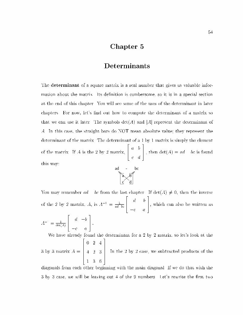
54
Chapter 5
Determinants
The determinant of a square matrix is a real number that gives us valuable infor-
mation about the matrix. Its de�nition is combersome, so it is in a special section
at the end of this chapter. You will see some of the uses of the determinant in later
chapters. For now, let's �nd out how to compute the determinant of a matrix so
that we can use it later. The symbols det(A) and jAj represent the determinant of
A. In this case, the straight bars do NOT mean absolute value; they represent the
determinant of the matrix. The determinant of a 1 by 1 matrix is simply the element
of the matrix. If A is the 2 by 2 matrix,
264 a b
c d
375 ; then det(A) = ad � bc is found
this way:
a b
c d
ad - bc
You may remember ad � bc from the last chapter. If det(A) 6= 0, then the inverse
of the 2 by 2 matrix, A, is A�1 = 1ad�bc
264 d �b
�c a
375, which can also be written as
A�1 = 1
det(A)
264 d �b
�c a
375 :
We have already found the determinant for a 2 by 2 matrix, so let's look at the
3 by 3 matrix A =
2666664
0 2 4
4 2 3
1 3 6
3777775. In the 2 by 2 case, we subtracted products of the
diagonals from each other beginning with the main diagonal. If we do that with the
3 by 3 case, we will be leaving out 4 of the 9 numbers. Let's rewrite the �rst two
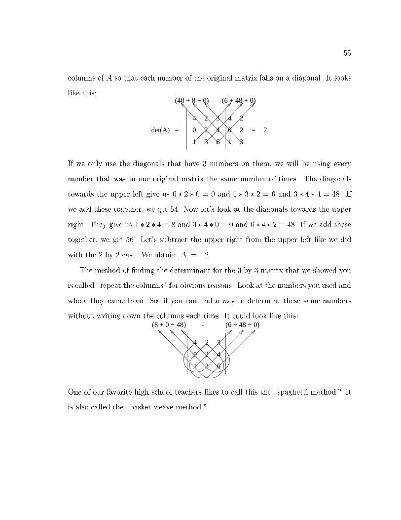
55
columns of A so that each number of the original matrix falls on a diagonal. It looks
like this:
4 2 3
0 2 4
1 3 6
4 2
0 2
1 3
= 2=det(A)
(48 + 8 + 0) - (6 + 48 + 0)
If we only use the diagonals that have 3 numbers on them, we will be using every
number that was in our original matrix the same number of times. The diagonals
towards the upper left give us 6 � 2 � 0 = 0 and 1 � 3 � 2 = 6 and 3 � 4 � 4 = 48. If
we add these together, we get 54. Now let's look at the diagonals towards the upper
right. They give us 1 � 2 � 4 = 8 and 3 � 4 � 0 = 0 and 6 � 4 � 2 = 48. If we add these
together, we get 56. Let's subtract the upper right from the upper left like we did
with the 2 by 2 case. We obtain jAj = �2.
The method of �nding the determinant for the 3 by 3 matrix that we showed you
is called \repeat the columns" for obvious reasons. Look at the numbers you used and
where they came from. See if you can �nd a way to determine these same numbers
without writing down the columns each time. It could look like this:
4 2 3
0 2 4
1 3 6
(8 + 0 + 48) - (6 + 48 + 0)
One of our favorite high school teachers likes to call this the \spaghetti method." It
is also called the \basket weave method."
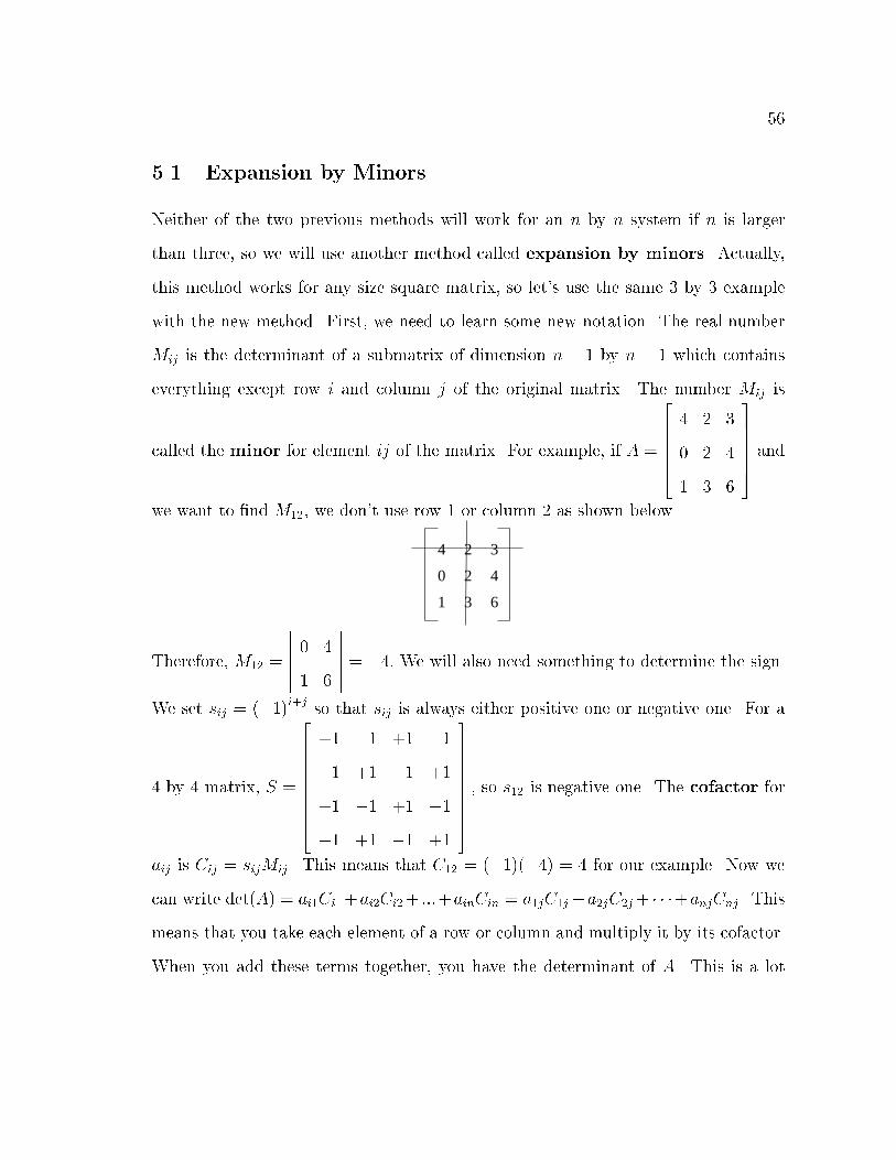
56
5.1 Expansion by Minors
Neither of the two previous methods will work for an n by n system if n is larger
than three, so we will use another method called expansion by minors. Actually,
this method works for any size square matrix, so let's use the same 3 by 3 example
with the new method. First, we need to learn some new notation. The real number
Mij is the determinant of a submatrix of dimension n � 1 by n � 1 which contains
everything except row i and column j of the original matrix. The number Mij is
called the minor for element ij of the matrix. For example, if A =
2666664
4 2 3
0 2 4
1 3 6
3777775and
we want to �nd M12; we don't use row 1 or column 2 as shown below.
4 2 3
0 2 4
1 3 6
Therefore, M12 =
�������0 4
1 6
�������= �4: We will also need something to determine the sign.
We set sij = (�1)i+j
so that sij is always either positive one or negative one. For a
4 by 4 matrix, S =
26666666664
+1 �1 +1 �1
�1 +1 �1 +1
+1 �1 +1 �1
�1 +1 �1 +1
37777777775; so s12 is negative one. The cofactor for
aij is Cij = sijMij. This means that C12 = (�1)(�4) = 4 for our example. Now we
can write det(A) = ai1Ci1+ai2Ci2+ :::+ainCin = a1jC1j+a2jC2j+ � � �+anjCnj. This
means that you take each element of a row or column and multiply it by its cofactor.
When you add these terms together, you have the determinant of A. This is a lot
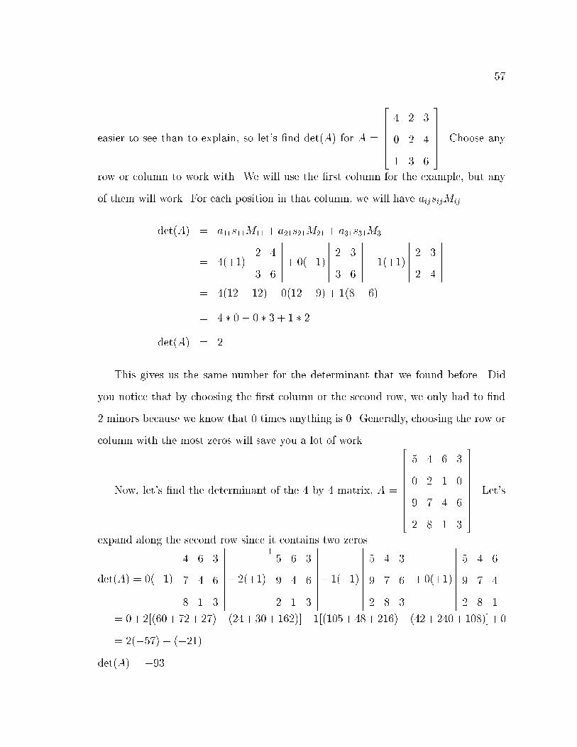
57
easier to see than to explain, so let's �nd det(A) for A =
2666664
4 2 3
0 2 4
1 3 6
3777775. Choose any
row or column to work with. We will use the �rst column for the example, but any
of them will work. For each position in that column, we will have aijsijMij.
det(A) = a11s11M11 + a21s21M21 + a31s31M31
= 4(+1)
�������2 4
3 6
�������+ 0(�1)
�������2 3
3 6
�������+ 1(+1)
�������2 3
2 4
�������= 4(12� 12)� 0(12� 9) + 1(8� 6)
= 4 � 0� 0 � 3 + 1 � 2
det(A) = 2
This gives us the same number for the determinant that we found before. Did
you notice that by choosing the �rst column or the second row, we only had to �nd
2 minors because we know that 0 times anything is 0. Generally, choosing the row or
column with the most zeros will save you a lot of work.
Now, let's �nd the determinant of the 4 by 4 matrix, A =
26666666664
5 4 6 3
0 2 1 0
9 7 4 6
2 8 1 3
37777777775. Let's
expand along the second row since it contains two zeros.
det(A) = 0(�1)
�����������
4 6 3
7 4 6
8 1 3
�����������+2(+1)
�����������
5 6 3
9 4 6
2 1 3
�����������+1(�1)
�����������
5 4 3
9 7 6
2 8 3
�����������+0(+1)
�����������
5 4 6
9 7 4
2 8 1
�����������= 0+2[(60+72+27)� (24+30+162)]�1[(105+48+216)� (42+240+108)]+0
= 2(�57)� (�21)
det(A) = �93

58
Expansion by minors will allow you to �nd the determinant of a square matrix of
any size. However, it requires a lot of operations when the matrix is large because
each submatix used to determine a minor must be expanded. In fact, �nding the
determinant using this method requires n! operations which is a very large number
when n is large because n! = n � (n� 1) � (n� 2) � : : : � 2 � 1.
5.2 Using Gaussian Elimination
The determinant can also be found using EROs in a manner similar to Gaussian
elimination. In order to use EROs to �nd the determinant of a matrix, you must
know a few facts about the determinant:
1. Interchanging two rows changes the sign of the determinant.
2. Multiplying a row by a scalar multiplies the determinant by that scalar.
3. Replacing any row by the sum of that row and any other row does NOT change
the determinant.
4. The determinant of a triangular matrix (upper or lower triangular) is the prod-
uct of the diagonal elements.
You can demonstrate these facts to yourself using a 2 by 2 matrix. Just as using
EROs does not change the solution to a system, EROs combined with these rules will
allow us to �nd the determinant of the original matrix. The use of EROs results in
a system that is equivalent to the original system, so if we apply these rules to the
determinant as we change the system, we will �nd the determinant to the original
coe�cient matrix. Let's use these rules to �nd the determinant of a 2 by 2 matrix. As
we work this problem, we will let Di represent the determinant of the current matrix
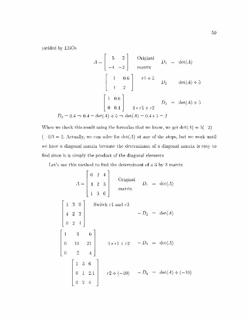
59
yielded by EROs
A =
264 5 3
�4 �2
375 Original
matrixD1 = det(A)
264 1 0:6
�4 �2
375 r1� 5
D2 = det(A)� 5
264 1 0:6
0 0:4
375
4 � r1 + r2D3 = det(A)� 5
D3 = 0:4) 0:4 = det(A) � 5) det(A) = 0:4 � 5 = 2
When we check this result using the formulas that we know, we get det(A) = 5(�2)�
(�4)3 = 2: Actually, we can solve for det(A) at any of the steps, but we work until
we have a diagonal matrix because the determinant of a diagonal matrix is easy to
�nd since it is simply the product of the diagonal elements.
Let's use this method to �nd the determinant of a 3 by 3 matrix.
A =
2666664
0 2 4
4 2 3
1 3 6
3777775
Original
matrixD1 = det(A)
2666664
1 3 6
4 2 3
0 2 4
3777775
Switch r1 and r3
�D2 = det(A)
2666664
1 3 6
0 �10 �21
0 2 4
3777775 �4 � r1 + r2 �D3 = det(A)
2666664
1 3 6
0 1 2:1
0 2 4
3777775 r2� (�10) �D4 = det(A)� (�10)

60
2666664
1 3 6
0 1 2:1
0 0 �0:2
3777775
�2 � r2 + r3
�D5 = det(A)� (�10)
D5 = �0:2
) �(�0:2) = det(A)� (�10)
) det(A) = (�10) � (0:2) = �2
We can verify this with either of the methods that we learned earlier to �nd the
determinant of a matrix.
Using only these small examples might lead you to think that it is slower to �nd
the determinant using elementary row operations. However, it actually requires fewer
steps for larger problems than does expansion by minors. Therefore, this method is
used more often to �nd the determinant in computational mathematics.
5.3 Inverses and Solutions to Systems
Determinants also provide another way to solve the system Ax = b. The method we
are going to describe is called Cramer's rule. We need one more bit of notation. We
will call the matrix A with the ith column replaced by the vector b, Bi. Let's use
the example that we worked with in Chapter 4. Matrix A =
264 5 3
�4 �2
375 and b =
264 93
�66
375. Matrix B1 =
264 93 3
�66 �2
375. Notice that the �rst column of A was replaced
by the vector b. Replace the second column of A with b to get B2 =
264 5 93
�4 �66
375.
We need to �nd the determinants of each of these matrices. We �nd that jAj = 2,
jB1j = 12, and jB2j = 42. The formula for Cramer's rule is xi =jBij
jAj. Therefore,
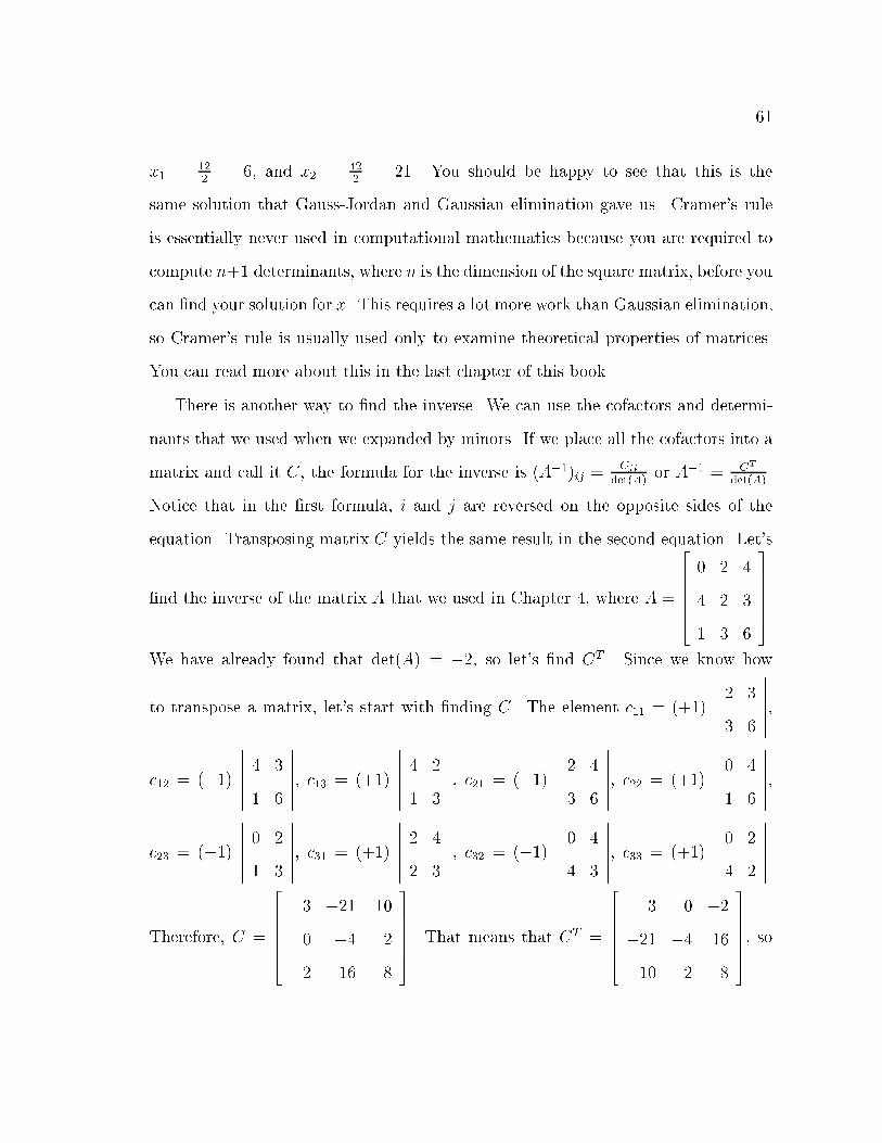
61
x1 = 122
= 6, and x2 = 422
= 21. You should be happy to see that this is the
same solution that Gauss-Jordan and Gaussian elimination gave us. Cramer's rule
is essentially never used in computational mathematics because you are required to
compute n+1 determinants, where n is the dimension of the square matrix, before you
can �nd your solution for x. This requires a lot more work than Gaussian elimination,
so Cramer's rule is usually used only to examine theoretical properties of matrices.
You can read more about this in the last chapter of this book.
There is another way to �nd the inverse. We can use the cofactors and determi-
nants that we used when we expanded by minors. If we place all the cofactors into a
matrix and call it C, the formula for the inverse is (A�1)ij =Cji
det(A)or A�1 = CT
det(A).
Notice that in the �rst formula, i and j are reversed on the opposite sides of the
equation. Transposing matrix C yields the same result in the second equation. Let's
�nd the inverse of the matrix A that we used in Chapter 4, where A =
2666664
0 2 4
4 2 3
1 3 6
3777775.
We have already found that det(A) = �2, so let's �nd CT . Since we know how
to transpose a matrix, let's start with �nding C. The element c11 = (+1)
�������2 3
3 6
�������,
c12 = (�1)
�������4 3
1 6
�������, c13 = (+1)
�������4 2
1 3
�������, c21 = (�1)
�������2 4
3 6
�������, c22 = (+1)
�������0 4
1 6
�������,
c23 = (�1)
�������0 2
1 3
�������, c31 = (+1)
�������2 4
2 3
�������, c32 = (�1)
�������0 4
4 3
�������, c33 = (+1)
�������0 2
4 2
�������.
Therefore, C =
2666664
3 �21 10
0 �4 2
�2 16 �8
3777775. That means that CT =
2666664
3 0 �2
�21 �4 16
10 2 �8
3777775, so
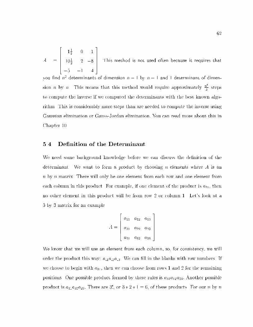
62
A�1 =
2666664
�112
0 1
1012
2 �8
�5 �1 4
3777775. This method is not used often because it requires that
you �nd n2 determinants of dimension n � 1 by n � 1 and 1 determinant of dimen-
sion n by n. This means that this method would require approximately n5
3steps
to compute the inverse if we computed the determinants with the best known algo-
rithm. This is considerably more steps than are needed to compute the inverse using
Gaussian elimination or Gauss-Jordan elimination: You can read more about this in
Chapter 10.
5.4 De�nition of the Determinant
We need some background knowledge before we can discuss the de�nition of the
determinant. We want to form a product by choosing n elements where A is an
n by n matrix. There will only be one element from each row and one element from
each column in this product. For example, if one element of the product is a21, then
no other element in this product will be from row 2 or column 1. Let's look at a
3 by 3 matrix for an example.
A =
2666664
a11 a12 a13
a21 a22 a23
a31 a32 a33
3777775
We know that we will use an element from each column, so, for consistency, we will
order the product this way: a 1a 2a 3. We can �ll in the blanks with row numbers. If
we choose to begin with a31; then we can choose from rows 1 and 2 for the remaining
positions. One possible product formed by these rules is a31a12a23: Another possible
product is a11a32a23: There are 3!, or 3 � 2 � 1 = 6; of these products. For our n by n

63
matrix, there are n! possible products. All 6 possible products for this 3 by 3 matrix
are: a11a22a33, a21a32a13, a31a12a23, a31a22a13, a21a12a33, and a11a32a23.
Now, we need to determine which sign (+ or �) should be attached to each prod-
uct. To do this, you need to order the product with the column numbers increasing as
we did above and look at the sequences of row numbers. For the product, a11a22a33;
we look at the row sequence (1,2,3). We are looking for inversions, or numbers that
are out of order. Since 1 comes before 2, 1 comes before 3, and 2 comes before 3 in
the sequence, there are no inversions in this sequence. In the sequence (2,3,1), which
comes from the product a21a32a13, there are two inversions because 2 is placed before
1 and 3 is placed before 1. There are also two inversions for the sequence from the
product a31a12a23: There are three inversions for (3,2,1) and one inversion each for
(2,1,3) and (1,3,2). If the number of inversions is even, then the sign attached to
the product is positive. If the number of inversions is odd, then the sign attached
to the product is negative. Notice that we did not say that the product was posi-
tive or negative. We simply are determining whether the product will be added or
subtracted.
De�nition 5.1 The determinant of a square matrix is the sum of all
the n! possible signed products formed from the matrix using each row
and each column only once for each product. The sign to be attached
to the product is the same as the one determined by the formula (�1)N
where N is the number of inversions as described above.
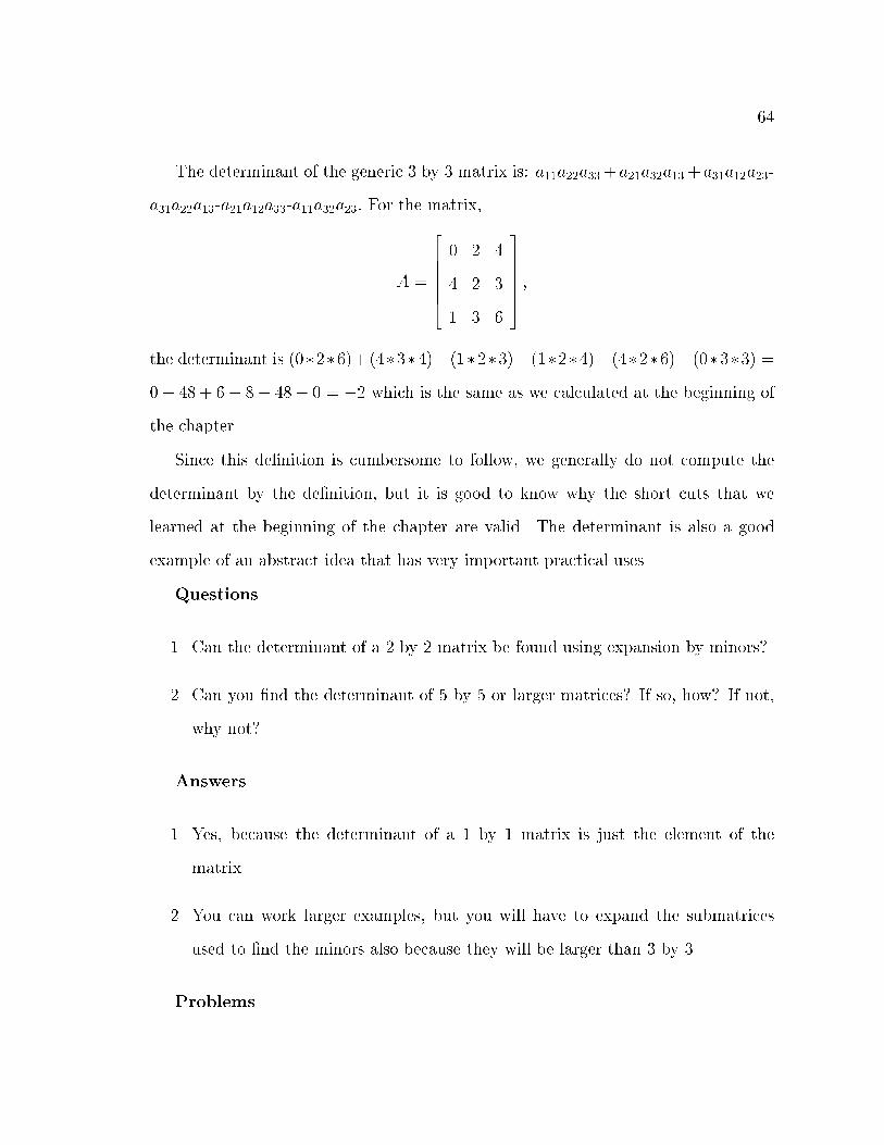
64
The determinant of the generic 3 by 3 matrix is: a11a22a33+a21a32a13+a31a12a23-
a31a22a13-a21a12a33-a11a32a23: For the matrix,
A =
2666664
0 2 4
4 2 3
1 3 6
3777775;
the determinant is (0�2�6)+(4�3�4)+(1�2�3)�(1�2�4)�(4�2�6)�(0�3�3) =
0 + 48 + 6� 8� 48� 0 = �2 which is the same as we calculated at the beginning of
the chapter.
Since this de�nition is cumbersome to follow, we generally do not compute the
determinant by the de�nition, but it is good to know why the short cuts that we
learned at the beginning of the chapter are valid. The determinant is also a good
example of an abstract idea that has very important practical uses.
Questions
1. Can the determinant of a 2 by 2 matrix be found using expansion by minors?
2. Can you �nd the determinant of 5 by 5 or larger matrices? If so, how? If not,
why not?
Answers
1. Yes, because the determinant of a 1 by 1 matrix is just the element of the
matrix.
2. You can work larger examples, but you will have to expand the submatrices
used to �nd the minors also because they will be larger than 3 by 3.
Problems

65
1. Find the determinants of these matrices. Show your work.
(a)
264 3 4
1 �2
375
(b)
264 5 �2
3 6
375
(c)
2666664
3 0 4
6 2 �1
5 �7 3
3777775
(d)
2666664
2 �3 1
7 0 5
�5 2 4
3777775
(e)
2666664
5 0 1
0 9 1
3 �5 0
3777775
(f)
26666666664
3 �2 7 6
�4 0 2 1
5 2 0 �2
2 0 �1 0
37777777775
(g)
26666666664
1 8 �3 2
9 3 0 1
�2 6 0 �4
2 �1 0 4
37777777775

66
(h)
26666666664
7 3 1 0
�2 �5 6 2
0 8 �3 1
2 0 0 �1
37777777775
(i)
266666666666664
1 0 2 0 4
6 0 9 3 7
3 0 5 0 1
5 2 7 9 8
6 0 4 0 3
377777777777775
2. Use Cramer's rule to solve these systems of equations:
(a)
2x1 + 3x2 � 5x3 = �11
�4x1 � x2 + 3x3 = 3
3x1 � 2x2 + x3 = 7
(b)
x1 � 5x2 + 7x3 = �10
9x2 + 2x3 = 7
x1 + 3x2 � x3 = 6
3. Find the inverse of matrix A using cofactors and determinants. Verify that you
found the inverse by checking that I is the product matrix of AA�1 or A�1A.
Remember, since A is square, you do not have to check both because if AA�1

67
or A�1A is the identity matrix, then so is the other.
A =
2666664
1 3 �1
4 �1 3
3 �2 1
3777775
4. Prove whether the following statements are true or false for 2 by 2 matrices.
Remember that a counterexample establishes that a statement is false.
(a) det(AB) = det(A) det(B)
(b) det(A�1) = 1det(A)
(c) det(A +B) = det(A) + det(B)
(d) det(AT ) = det(A)
Remark 14 In general, you may NOT assume that a statement is
true for all matrices just because it is true for 2 by 2 matrices, but for
the examples in this question, those that are true for 2 by 2 matrices
are true for all matrices if the dimensions allow the operations to be
performed.
5. Show that the determinant of an upper triangular matrix is the product of the
diagonal entries.
68
Chapter 6
Consistent and Inconsistent Systems
When you solve a system of linear equations, what does your solution set (all of your
solutions) describe geometrically? In each problem involving 2 by 2 matrices that we
solved, our solution set was the point of intersection of the two lines represented by
the equations in our system. In each problem with 3 by 3 matrices, the solution set
was the point of intersection of 3 planes. However, a system of linear equations does
not always have a point as the solution set.
If you solve the system
x1 + 2x2 = 4
2x1 + 4x2 = 8
algebraically, what do you get? You have an in�nite number of solutions along the
line x1 = 4 � 2x2 because any solution to the �rst equation, also solves the second
equation. Therefore, you can choose any value for one of the variables, and you will
be able to �nd a value for the other variable so that both equations are satis�ed. This
is called a consistent system because there is a solution. It is further categorized as
an underdetermined system because there is not enough information to determine
a unique solution.
De�nition 6.1 A system is consistent if there is at least one solution.
De�nition 6.2 A system is underdetermined when there are an in�-
nite number of solutions.
For a linear system, if there are two or more solutions, then there are an in�nite
number of solutions. These solutions all lie on the same line. Geometrically, this
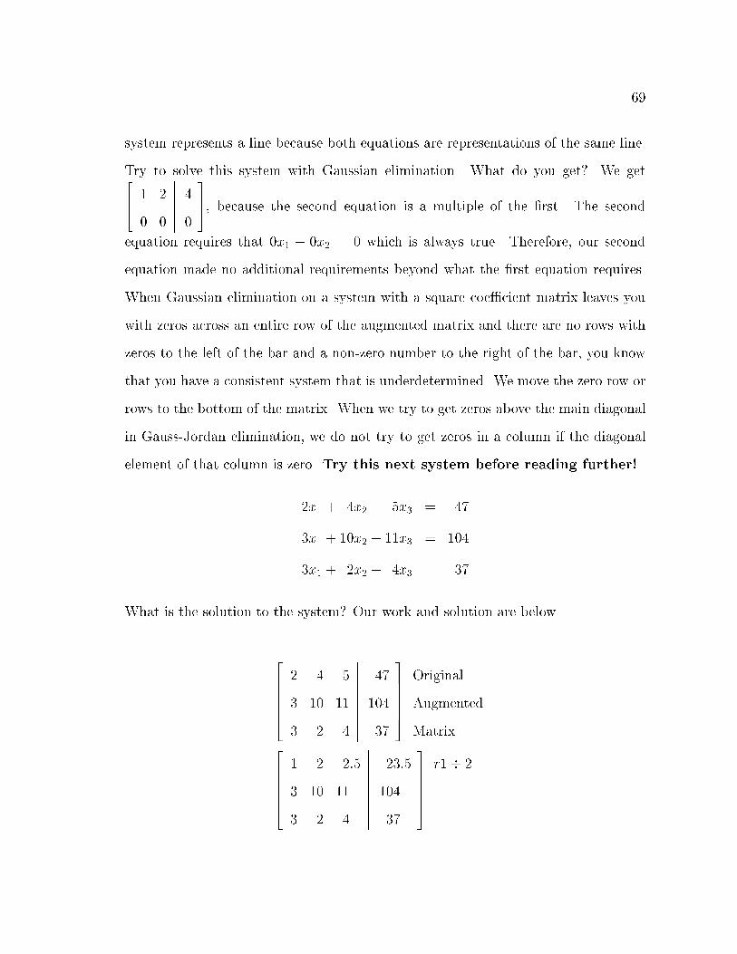
69
system represents a line because both equations are representations of the same line.
Try to solve this system with Gaussian elimination. What do you get? We get264 1 2
0 0
�������4
0
375, because the second equation is a multiple of the �rst. The second
equation requires that 0x1 + 0x2 = 0 which is always true. Therefore, our second
equation made no additional requirements beyond what the �rst equation requires.
When Gaussian elimination on a system with a square coe�cient matrix leaves you
with zeros across an entire row of the augmented matrix and there are no rows with
zeros to the left of the bar and a non-zero number to the right of the bar, you know
that you have a consistent system that is underdetermined. We move the zero row or
rows to the bottom of the matrix. When we try to get zeros above the main diagonal
in Gauss-Jordan elimination, we do not try to get zeros in a column if the diagonal
element of that column is zero. Try this next system before reading further!
2x1 + 4x2 + 5x3 = 47
3x1 + 10x2 + 11x3 = 104
3x1 + 2x2 + 4x3 = 37
What is the solution to the system? Our work and solution are below.
2666664
2 4 5
3 10 11
3 2 4
�����������
47
104
37
3777775
Original
Augmented
Matrix2666664
1 2 2:5
3 10 11
3 2 4
�����������
23:5
104
37
3777775
r1� 2

70
2666664
1 2 2:5
0 4 3:5
0 �4 �3:5
�����������
23:5
33:5
�33:5
3777775 �3 � r1 + r2
�3 � r1 + r32666664
1 2 2:5
0 1 :875
0 �4 �3:5
�����������
23:5
8:375
�33:5
3777775 r2� 4
2666664
1 2 2:5
0 1 :875
0 0 0
�����������
23:5
8:375
0
3777775
4 � r2 + r32666664
1 0 0:75
0 1 0:875
0 0 0
�����������
6:75
8:375
0
3777775
�2 � r2 + r1
This tells us that x1 = 6:75 � :75x3 and x2 = 8:375 � :875x3. That means that
we can choose whatever number we want for one element of x and get corresponding
valid solutions for the other two. For instance, if we choose x3 to be 1, then x1 = 6
and x2 = 7:5. Instead, we may choose x1 = 6:75 then x2 = 8:375 and x3 = 0. There
are an in�nite number of solutions that we can �nd in this manner. Notice that this
system is also consistent and underdetermined.
What do you get if you try to solve
x1 + 2x2 = 4
2x1 + 4x2 = 9
algebraically? The result is a requirement that you know cannot be satis�ed. We
get 0 = 1 (you may arrive at a di�erent contradictory requirement). This system is
called inconsistent.
De�nition 6.3 A system is inconsistent if it has no solutions.
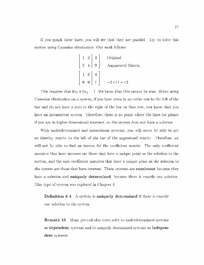
71
If you graph these lines, you will see that they are parallel. Try to solve this
system using Gaussian elimination. Our work follows:
264 1 2
2 4
�������4
9
375 Original
Augmented Matrix264 1 2
0 0
�������4
1
375
�2 � r1 + r2
This requires that 0x1+0x2 = 1. We know that this cannot be true. When using
Gaussian elimination on a system, if you have zeros in an entire row to the left of the
bar and do not have a zero to the right of the bar on that row, you know that you
have an inconsistent system. Therefore, there is no point where the lines (or planes
if you are in higher dimensions) intersect, so the system does not have a solution.
With underdetermined and inconsistent systems, you will never be able to get
an identity matrix to the left of the bar of the augmented matrix. Therefore, we
will not be able to �nd an inverse for the coe�cient matrix. The only coe�cient
matrices that have inverses are those that have a unique point as the solution to the
system, and the only coe�cient matrices that have a unique point as the solution to
the system are those that have inverses. These systems are consistent because they
have a solution and uniquely determined because there is exactly one solution.
This type of system was explored in Chapter 4.
De�nition 6.4 A system is uniquely determined if there is exactly
one solution to the system.
Remark 15 Many pre-calculus texts refer to underdetermined systems
as dependent systems and to uniquely determined systems as indepen-
dent systems.
72
For the examples above, �nd the determinant of A in each case. Can you draw
a conclusion from this data that relates the determinant of A to whether or not the
system has a unique solution? If not, solve some additional systems and try again to
draw a conclusion.
Using determinants, we can check to see if a system is uniquely determined. If
the determinant of the coe�cient matrix is not equal to zero, the system is uniquely
determined. Thinking of the systems that involve 2 by 2 matrices, can you tell why
systems with determinants equal to zero are not uniquely determined? Remember
that the formula for the inverse of a 2 by 2 matrix is 1det(A)
264 d �b
�c a
375 : Does 1
det(A)
have a meaning if det(A) = 0? No, it does not. This is another illustration of the
fact that the square matrix represented by A in Ax = b for an inconsistent or under-
determined systems does not have an inverse. You will see that this holds true for
all the problems that you do. If det(A) 6= 0; the system is uniquely determined
and A is invertible. If det(A) = 0, the system is either underdetermined
or inconsistent; therefore, A is not invertible. In practice, the determinant is
not used to test systems in this manner because other methods require fewer steps.
However, these relationships are very important to the theory of matrices.
Remark 16 In this section, occasionally, we refer to systems that have
square coe�cient matrices. This is only for simplicity. All of these clas-
si�cations also apply to matrices with non-square coe�cient matrices.
However, we cannot take the determinant of a non-square matrix. Also,
we cannot rely entirely upon the appearance of the last row of the system
after Gaussian elimination eventhough that information is still valuable.
Here is a visual breakdown of the information that you have been given. This
breakdown assumes a square coe�cient matrix.
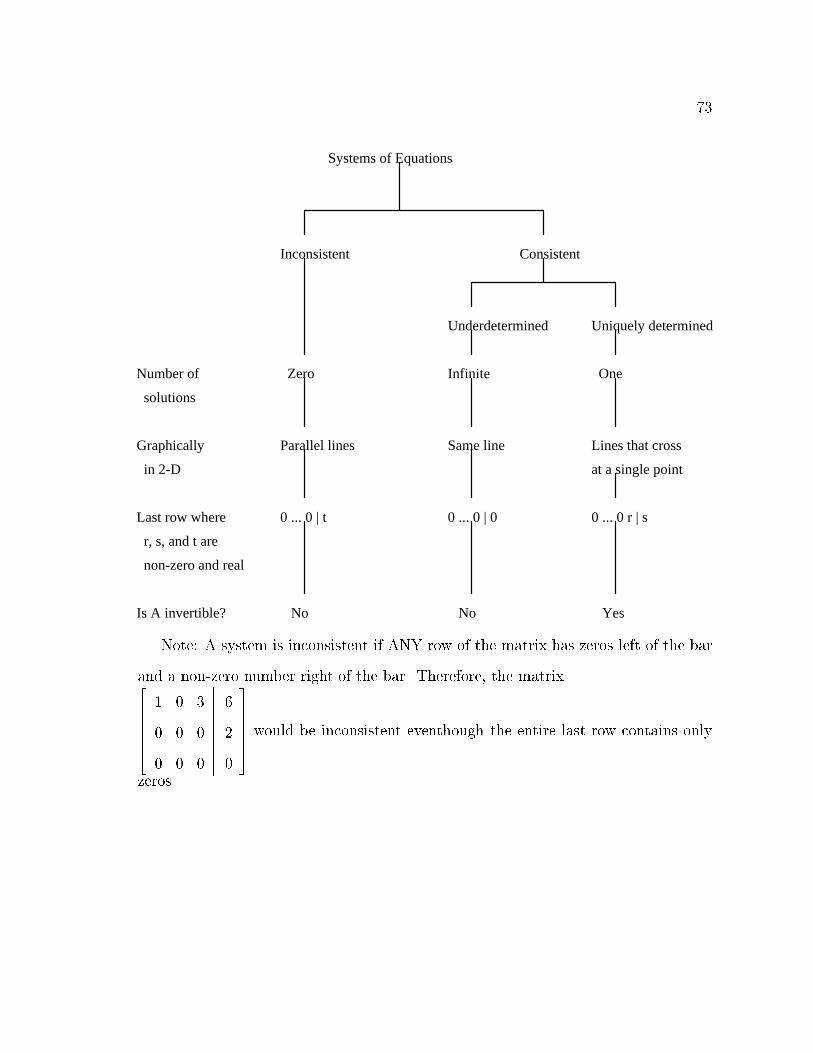
73
Systems of Equations
Inconsistent
Infinite One Zero
Consistent
Number of
solutions
No No Yes
non-zero and real
r, s, and t are
Last row where 0 ... 0 | t 0 ... 0 | 0 0 ... 0 r | s
in 2-D
Graphically Parallel lines Same line
at a single point
Lines that cross
Is A invertible?
Underdetermined Uniquely determined
Note: A system is inconsistent if ANY row of the matrix has zeros left of the bar
and a non-zero number right of the bar. Therefore, the matrix2666664
1 0 3
0 0 0
0 0 0
�����������
6
2
0
3777775would be inconsistent eventhough the entire last row contains only
zeros.

74
Problems
1. Classify these systems as either consistent or inconsistent. If the system is
consistent, further categorize it as underdetermined or uniquely determined.
Explain why the system �ts into that category. Also, explain what this means
graphically for each system.
(a) 2x1 + 3x2 = 9 and 3x1 + 412x2 = 13
(b) 3x1 + 4x2 = 7 and 9x1 + 12x2 = 21
(c) 2x1 + 3x2 = 8 and 3x1 + 4x2 = 11
(d) Ax = b where A =
2666664
1 3 4
2 1 6
1 �7 0
3777775and b =
2666664
5
6
�3
3777775
(e) Ax = b where A =
2666664
2 3 4
5 2 �1
0 �11 18
3777775and b =
2666664
5
7
11
3777775
(f) Ax = b where A =
2666664
4 2 6
1 12
112
6 3 9
3777775and b =
2666664
�2
�12
�3
3777775
(g) Ax = b where A =
2666664
2 3 4
1 2 3
3 412
6
3777775and b =
2666664
9
6
13
3777775
2. Which of the matrices in problem 1 are invertible?

75
First Review
1. What are the dimensions of matrix A?
A =
264 3 2 5
7 1 0
375
2. Construct a generic 3 by 4 matrix, B, using the correct subscripted notation.
(Hint: The element in the upper left corner is b11:)
3. (a) Put the following information into a 2 by 3 matrix and label it.
Keith scored 94 on his test and had a 99 homework average. Juan received
75 on his test and averaged 80 on homework. Yolanda's homework average
was 90, but she scored 70 on the test.
(b) Transpose the matrix in problem 3a and attach labels.
4. Consider the matrices
A =
2666664
4 3 9
0 �1 5
10 2 �8
3777775and B =
2666664
9 �2 6
8 0 1
�3 12 7
3777775:
(a) What is A+B?
(b) What is AT +B?
5. If matrix B is symmetric does A +B = A+BT ? Why or why not?
6. To raise money, our high school band decided to sell candy. They sold candy
with nuts (N) and plain chocolate (P). Hoping to inspire people to sell candy,
the band director held a contest among the grade levels to see which grade

76
would sell the most candy. The contest lasted for 3 weeks. Here are the results
from the �rst two weeks. The numbers represent packages sold:
Fresh:
Soph:
Jr:
Sr:
N P26666666664
400 350
300 350
350 300
200 250
37777777775=W1
Fresh:
Soph:
Jr:
Sr:
N P26666666664
300 300
200 250
300 200
250 200
37777777775=W2
(a) How much of each kind of candy had each grade level sold by the end of
the second week?
(b) Which grade level was leading the contest?
(c) By the end of the third week, the totals were:
Fresh:
Soph:
Jr:
Sr:
N P26666666664
1000 850
700 750
900 700
600 600
37777777775= T
How much of each kind of candy did each grade level sell during the third
week?
(d) How many packages of plain chocolate were sold during the three-week
period by the band?
(e) If the band makes 30 cents pro�t from each package of candy with nuts
and makes 20 cents pro�t from each package of plain chocolate, how much
pro�t did each grade level make? Answer this question using matrices.
(f) How much total pro�t did the band make from this venture? Please write
your answer in dollars.
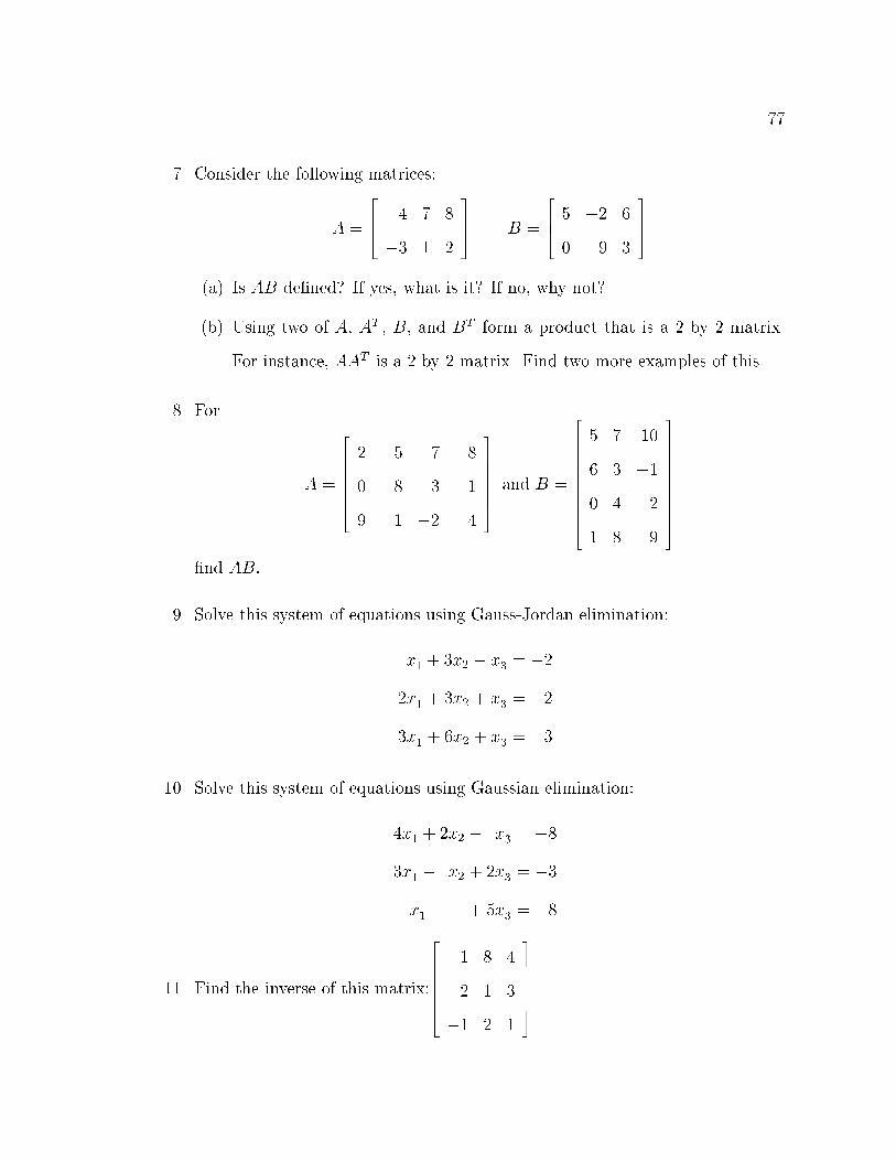
77
7. Consider the following matrices:
A =
264 4 7 8
�3 1 2
375 B =
264 5 �2 6
0 9 3
375
(a) Is AB de�ned? If yes, what is it? If no, why not?
(b) Using two of A; AT; B; and B
T form a product that is a 2 by 2 matrix.
For instance, AAT is a 2 by 2 matrix. Find two more examples of this.
8. For
A =
2666664
2 5 7 8
0 �8 3 �1
9 1 �2 4
3777775and B =
26666666664
5 7 10
6 3 �1
0 4 2
1 8 9
37777777775
�nd AB:
9. Solve this system of equations using Gauss-Jordan elimination:
x1 + 3x2 � x3 = �2
2x1 + 3x2 + x3 = 2
3x1 + 6x2 + x3 = 3
10. Solve this system of equations using Gaussian elimination:
4x1 + 2x2 � x3 = �8
3x1 � x2 + 2x3 = �3
x1 + 5x3 = 8
11. Find the inverse of this matrix:
2666664
1 8 4
2 1 3
�1 2 1
3777775

78
12. Does the inverse of a matrix always exist? Explain.
13. Find the determinant of these matrices. Show your work when possible.
(a)
264 4 6
�1 �2
375
(b)
2666664
4 8 2
�1 0 3
9 6 1
3777775
(c)
26666666664
7 9 2 �6
�5 4 0 4
2 1 1 6
3 7 0 2
37777777775
(d)
266666666666664
6 6 0 0 1
�9 �8 0 4 7
5 6 2 5 9
0 3 0 0 0
1 10 0 0 1
377777777777775
14. Identify the following as consistent or inconsistent. If the system is consistent,
further categorize it as underdetermined or uniquely determined. Explain.
(a) Ax = b where A =
2666664
2 1 3
7 6 11
3 4 5
3777775and b =
2666664
4
10
2
3777775
(b)
2x1 + 3x2 + x3 = 10
4x1 + 2x2 = 10
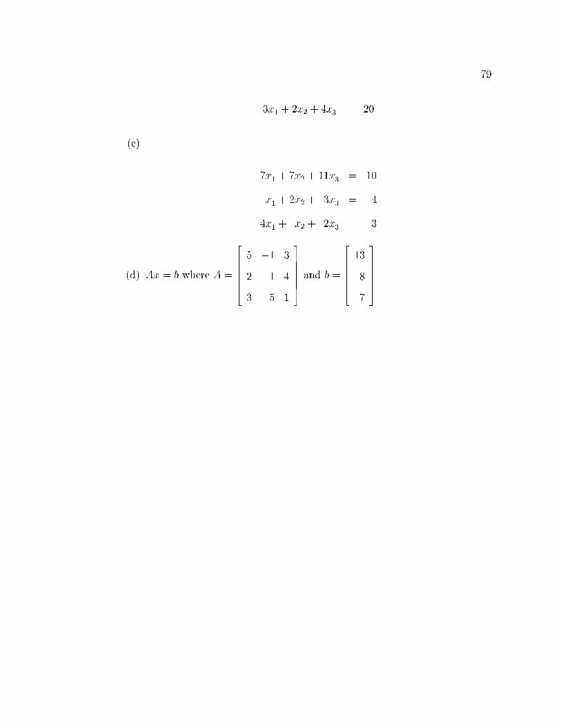
79
3x1 + 2x2 + 4x3 = 20
(c)
7x1 + 7x2 + 11x3 = 10
x1 + 2x2 + 3x3 = 4
4x1 + x2 + 2x3 = 3
(d) Ax = b where A =
2666664
5 �1 3
2 1 4
3 5 1
3777775and b =
2666664
13
8
7
3777775
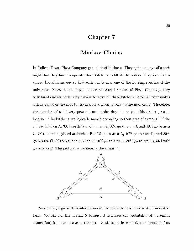
80
Chapter 7
Markov Chains
In College Town, Pizza Company gets a lot of business. They get so many calls each
night that they have to operate three kitchens to �ll all the orders. They decided to
spread the kitchens out so that each one is near one of the housing sections of the
university. Since the same people own all three branches of Pizza Company, they
only hired one set of delivery drivers to serve all three kitchens. After a driver makes
a delivery, he or she goes to the nearest kitchen to pick up the next order. Therefore,
the location of a delivery person's next order depends only on his or her present
location. The kitchens are logically named according to their area of campus. Of the
calls to kitchen A, 30% are delivered in area A, 30% go to area B, and 40% go to area
C. Of the orders placed at kitchen B, 40% go to area A, 40% go to area B, and 20%
go to area C. Of the calls to kitchen C, 50% go to area A, 30% go to area B, and 20%
go to area C. The picture below depicts the situation.
A C
B
.3
.4
.2
.2
.3
.3
.4
.4
.5
As you might guess, this information will be easier to read if we write it in matrix
form. We will call this matrix S because it expresses the probability of movement
(transition) from one state to the next. A state is the condition or location of an

81
object in the system at a particular time. Therefore, our diagram is called a state
diagram. Matrices of this type are called transition matrices. Our labeled transition
matrix looks like this:
A
B
C
A B C2666664
:3 :3 :4
:4 :4 :2
:5 :3 :2
3777775= S
For each element, Sij, i represents the starting location, and j represents the
ending location for that move. This means that the row is the beginning location,
and the column is the ending location after one move. We will want to learn things
about what will happen in the future to Pizza Company, and this situation has the
attributes necessary for what is called a Markov chain. Therefore, we will model the
problem as a Markov chain in order to obtain information about the future.
A problem can be considered a (homogeneous) Markov chain if it has the fol-
lowing properties:
(a) For each time period, every object (person) in the system is in exactly one of
the de�ned states. At the end of each time period, each object either moves to
a new state or stays in that same state for another period.
(b) The objects move from one state to the next according to the transition proba-
bilities which depend only on the current state (they do not take any previous
history into account). The total probability of movement from a state (move-
ment from a state to the same state does count as movement) must equal one.
(c) The transition probabilities do not change over time (the probability of going
from state A to state B today is the same as it will be at any time in the future).

82
Remark 17 Requirement (c) is not a requirement of Markov chains in
general. It is a requirement for a special kind of Markov chain called
a homogeneous Markov chain. We will be studying only homogeneous
Markov chains in this book, so we will use the term Markov chain to refer
to a homogeneous Markov chain.
The transition matrix used to model the Markov chain will have the following
properties:
(a) Each element of the transition matrix is a probability; therefore, each is a
number between 0 and 1, inclusive.
(b) The elements of each row of the transition matrix sum to 1. This is due to
property (b) of a Markov Chain.
(c) The transition matrix must be square because it has a row and a column for
each state.
We will assume that it takes each delivery person the same amount of time to
make one delivery. Therefore, after one delivery, of the cars that began in A, 30%
will again be in A, 30% will be in B, and 40% will be in C. Since we only have
three locations, and each delivery person must be somewhere after each delivery, the
probability that a car is in one of those three locations must be one. This is why
each row sums to 1. Because we are dealing with probabilities, each entry must be
between 0 and 1, inclusive. The most important fact that lets us model this situation
as a Markov chain is that the next location for delivery depends only on the current
location, not previous history. It is also true that our matrix of probabilities does not
change during the time we are observing.
83
Remark 18 Some assumptions are not completely accurate, but if we
did not make assumptions to generalize the problem, we would not have
the ability to approximate a solution to the problem. We just need to
make sure that our assumptions are reasonable. The assumption that
each delivery takes the same amount of time is reasonable if you consider
that the average delivery times should be nearly equal.
Now that you know the background, we can begin the fun part. Do you know
what the probability matrix would look like that describes where a car would be after
exactly 2 deliveries? What about 3, 4, or 5 deliveries? Can you predict the probability
matrix for the cars after a night of deliveries?
Well, lets start with a simpler question. If you begin at kitchen C, what is the
probability that you will be in area B after 2 deliveries? Think about how you can
get to B. We can go from C to C, then from C to B. We can go from C to B, then
from B to B. We can go from C to A, then from A to B. We will let P(CB) represent
the probability of going from C to B in one delivery. Let's write this probability in
our shorthand notation. Do you remember how probabilities work? If two (or more)
independent events must both (all) happen, we multiply their probabilities together.
If there are two (or more) distinct events that would both (all) work, we add the
probabilities of those events together.
Remark 19 Notice that we said we can multiply probabilities together
if the events are independent. We know that our events are independent
of one another because someone in area A is equally likely to order a
pizza whether or not someone in area B or C ordered a pizza. If our
events were not independent, we would not be able to simply multiply the
probabilities.
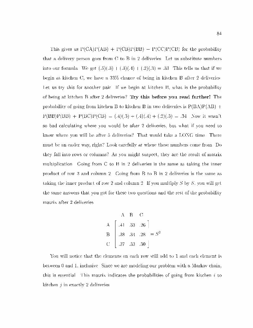
84
This gives us P(CA)P(AB) + P(CB)P(BB) + P(CC)P(CB) for the probability
that a delivery person goes from C to B in 2 deliveries. Let us substitute numbers
into our formula. We get (:5)(:3) + (:3)(:4) + (:2)(:3) = :33. This tells us that if we
begin at kitchen C, we have a 33% chance of being in kitchen B after 2 deliveries.
Let us try this for another pair. If we begin at kitchen B, what is the probability
of being at kitchen B after 2 deliveries? Try this before you read further! The
probability of going from kitchen B to kitchen B in two deliveries is P(BA)P(AB) +
P(BB)P(BB) + P(BC)P(CB) = (:4)(:3) + (:4)(:4) + (:2)(:3) = :34. Now it wasn't
so bad calculating where you would be after 2 deliveries, but what if you need to
know where you will be after 5 deliveries? That would take a LONG time. There
must be an easier way, right? Look carefully at where these numbers come from. Do
they fall into rows or columns? As you might suspect, they are the result of matrix
multiplication. Going from C to B in 2 deliveries is the same as taking the inner
product of row 3 and column 2. Going from B to B in 2 deliveries is the same as
taking the inner product of row 2 and column 2. If you multiply S by S, you will get
the same answers that you got for these two questions and the rest of the probability
matrix after 2 deliveries.
A
B
C
A B C2666664
:41 :33 :26
:38 :34 :28
:37 :33 :30
3777775= S
2
You will notice that the elements on each row still add to 1 and each element is
between 0 and 1, inclusive. Since we are modeling our problem with a Markov chain,
this is essential. This matrix indicates the probabilities of going from kitchen i to
kitchen j in exactly 2 deliveries.

85
Now that we have this matrix, it should be easier to �nd where we will be after
3 deliveries. We will let p(AB) represent the probability of going from A to B in
2 deliveries. Let's �nd the probability of going from C to B in 3 deliveries. The
probability is p(CA)P(AB) + p(CB)P(BB) + p(CC)P(CB) = (:37)(:3) + (:33)(:4) +
(:3)(:3) = :333. Where do these numbers come from? This probability is the inner
product of row three of S2 and column two of S. Therefore, if we multiply S2 by S,
we will get the probability matrix for 3 deliveries.
S2S = SSS = S
3 =
2666664
:385 :333 :282
:390 :334 :276
:393 :333 :274
3777775
By now, you probably know how we �nd the matrix of probabilities for 4, 5 or
more deliveries. Notice that the elements on each row still add to 1. Therefore, it
is important that you do not round your answers. Keep as many decimal places as
possible to retain accuracy.
S4 =
2666664
:3897 :3333 :2770
:3886 :3334 :2780
:3881 :3333 :2786
3777775
S5 =
2666664
:38873 :33333 :27794
:38894 :33334 :27772
:38905 :33333 :27762
3777775
S6 =
2666664
:388921 :333333 :277746
:388878 :333334 :277788
:388857 :333333 :277810
3777775

86
S7 =
2666664
:3888825 :3333333 :2777842
:3888910 :3333334 :2777756
:3888953 :3333333 :2777714
3777775
What do you notice about these matrices as we take into account more and more
deliveries? The numbers in each column seems to be converging to a particular
number. Think about what this tells us about our long term probabilities.
This tells us that after a large number of deliveries, it no longer matters which kitchen
we were in when we started. At the end of the evening, we have a 38:8% chance of
being at kitchen A, 33:3% chance of being at kitchen B, and 27:7% chance of being
in kitchen C. This convergence will happen with most of the transition matrices that
we consider.
Remark 20 If all the entries of the transition matrix are between 0
and 1 EXCLUSIVELY, then convergence is guaranteed to take place.
Convergence may take place when 0 and 1 are in the transition matrix,
but convergence is no longer guaranteed. For an example, look at the ma-
trix A =
264 0 1
1 0
375 : Think about the situation that this matrix represents
in order to understand why Ak oscillates as k grows.
Sometimes, you will be given a vector of initial distributions to describe how many
or what part of the objects are in each state in the beginning. Using this vector, you
can �nd out how many or what part of the objects are in each state at any later
time. If the initial distribution vector is a vector of decimals, it tells what part of the
total number of objects are in each state in the beginning. It contains only numbers
between 0 and 1, inclusive, and the elements in the row sum to one. Alternatively, the
vector of initial distributions could contain the actual number of objects or people in
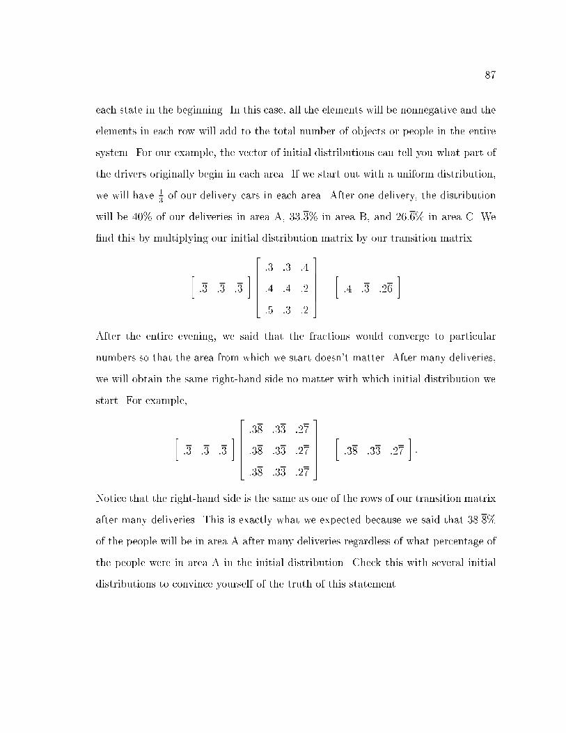
87
each state in the beginning. In this case, all the elements will be nonnegative and the
elements in each row will add to the total number of objects or people in the entire
system. For our example, the vector of initial distributions can tell you what part of
the drivers originally begin in each area. If we start out with a uniform distribution,
we will have 13of our delivery cars in each area. After one delivery, the distribution
will be 40% of our deliveries in area A, 33:3% in area B, and 26:6% in area C. We
�nd this by multiplying our initial distribution matrix by our transition matrix.
�:3 :3 :3
�2666664
:3 :3 :4
:4 :4 :2
:5 :3 :2
3777775=
�:4 :3 :26
�
After the entire evening, we said that the fractions would converge to particular
numbers so that the area from which we start doesn't matter. After many deliveries,
we will obtain the same right-hand side no matter with which initial distribution we
start. For example,
�:3 :3 :3
�2666664
:38 :33 :27
:38 :33 :27
:38 :33 :27
3777775=
�:38 :33 :27
�:
Notice that the right-hand side is the same as one of the rows of our transition matrix
after many deliveries. This is exactly what we expected because we said that 38.8%
of the people will be in area A after many deliveries regardless of what percentage of
the people were in area A in the initial distribution. Check this with several initial
distributions to convince yourself of the truth of this statement.
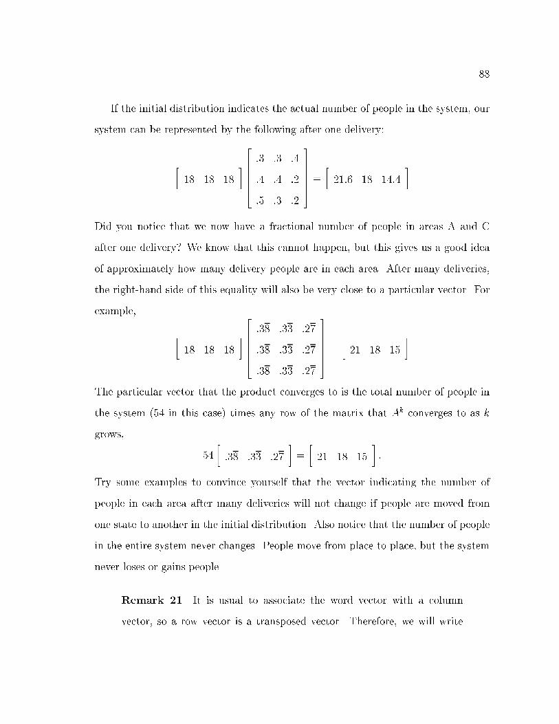
88
If the initial distribution indicates the actual number of people in the system, our
system can be represented by the following after one delivery:
�18 18 18
�2666664
:3 :3 :4
:4 :4 :2
:5 :3 :2
3777775=
�21:6 18 14:4
�
Did you notice that we now have a fractional number of people in areas A and C
after one delivery? We know that this cannot happen, but this gives us a good idea
of approximately how many delivery people are in each area. After many deliveries,
the right-hand side of this equality will also be very close to a particular vector. For
example,
�18 18 18
�2666664
:38 :33 :27
:38 :33 :27
:38 :33 :27
3777775=
�21 18 15
�
The particular vector that the product converges to is the total number of people in
the system (54 in this case) times any row of the matrix that Ak converges to as k
grows,
54
�:38 :33 :27
�=
�21 18 15
�:
Try some examples to convince yourself that the vector indicating the number of
people in each area after many deliveries will not change if people are moved from
one state to another in the initial distribution. Also notice that the number of people
in the entire system never changes. People move from place to place, but the system
never loses or gains people.
Remark 21 It is usual to associate the word vector with a column
vector, so a row vector is a transposed vector. Therefore, we will write

89
�18 18 18
�2666664
:3 :3 :4
:4 :4 :2
:5 :3 :2
3777775=
�21:6 18 14:4
�as xTA = b
T and
�18 18 18
�2666664
:38 :33 :27
:38 :33 :27
:38 :33 :27
3777775=
�21 18 15
�as xTAk = b
T where k
is a large whole number.
Remark 22 Some authors set up transition matrices so that j represents
the starting location and i represents the ending location. In these cases,
the columns add to one. For this case, the entire equation is transposed,
so instead of xTAk = bT where x is the column vector of initial distribution
and b is the column vector of distributions after k steps, the equation is
(Ak)Tx = b:
Questions
1. Using the data from our example, if Pizza Company has the money to enlarge
one of their kitchens, which kitchen should they enlarge?
2. If they have to close a kitchen, which one should they close?
Answers
1. Since almost 39% of their business comes from area A, Pizza Company should
enlarge kitchen A.
2. Since the least amount of their business comes from area C, that should be the
�rst to close.

90
Problems
1. Set up a matrix, similar to the matrices we used in this chapter, that corresponds
to this state diagram:
A C
B
.4
.2.7
.3
.1
.2 .3
.8
2. (a) Draw a picture corresponding to this transition matrix:
A
B
C
D
A B C D26666666664
:25 :15 :2 :4
0 :5 :5 0
0 0 1 0
:3 :4 :1 :2
37777777775
(b) Look closely at C in your picture. What do you notice that is strange
about the way information ows near C? What e�ect do you think this
might have on the long-range distribution of matter in this system?
3. Which of the following are transition matrices? Explain.
(a)
2666664
:4 :3 :3
:2 :4 :4
:6 :1 :3
3777775
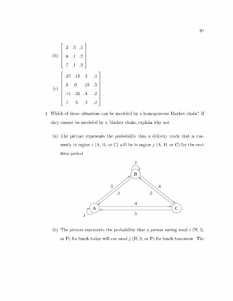
91
(b)
2666664
:2 :3 :5
:6 :1 :2
:7 :1 :3
3777775
(c)
26666666664
:25 :15 :3 :4
:5 0 :15 :3
:15 :35 :4 :2
:1 :5 :2 :2
37777777775
4. Which of these situations can be modeled by a homogeneous Markov chain? If
they cannot be modeled by a Markov chain, explain why not.
(a) The picture represents the probability that a delivery truck that is cur-
rently in region i (A, B, or C) will be in region j (A, B, or C) for the next
time period.
A C
B
.1
.1
.2 .5
.5 .6
.4
.5
(b) The picture represents the probability that a person eating meal i (H, S,
or P) for lunch today will eat meal j (H, S, or P) for lunch tomorrow. The

92
letter H stands for hamburger, S stands for salad, and P stands for pizza.
H
S
P
.2 .3
.2
.5 .6
.4.2
.3
.3
5. Look at the questions in problem 4. Write a sample transition matrix for the
problem or problems that can be modeled using a Markov chain.
6.
Assume S is the transition matrix
A
B
C
A B C2666664
:2 :3 :5
:4 :4 :2
:4 :6 0
3777775= S
(a) What is the probability of going from state A to state B in one step?
(b) What is the probability of going from state B to state C in exactly two
steps?
(c) What is the probability of going from state C to state A in exactly three
steps?
(d) Give the transition matrix, S2; for two steps (S2 would give the probabili-
ties of going from state i to state j in exactly 2 steps).
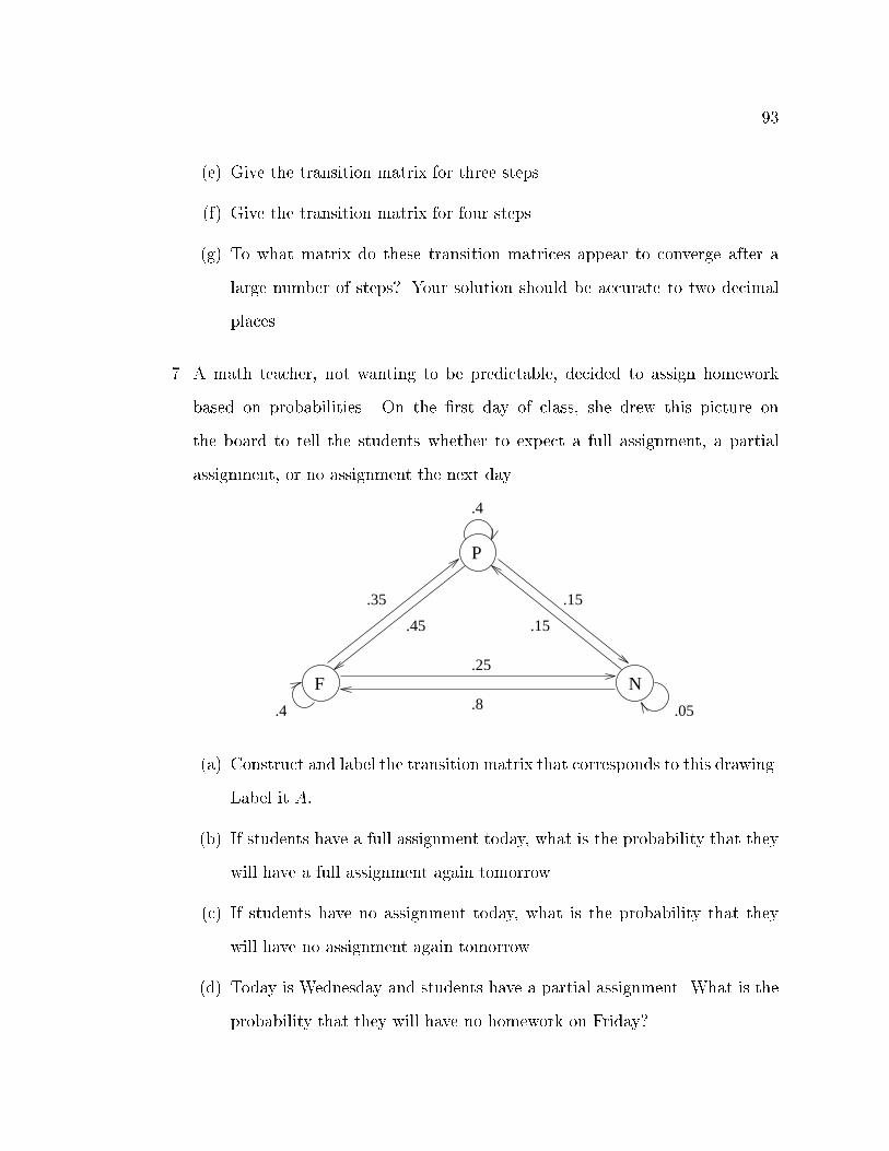
93
(e) Give the transition matrix for three steps.
(f) Give the transition matrix for four steps.
(g) To what matrix do these transition matrices appear to converge after a
large number of steps? Your solution should be accurate to two decimal
places.
7. A math teacher, not wanting to be predictable, decided to assign homework
based on probabilities. On the �rst day of class, she drew this picture on
the board to tell the students whether to expect a full assignment, a partial
assignment, or no assignment the next day.
F
P
N
.4 .05
.4
.25
.8
.15
.15.45
.35
(a) Construct and label the transition matrix that corresponds to this drawing.
Label it A:
(b) If students have a full assignment today, what is the probability that they
will have a full assignment again tomorrow.
(c) If students have no assignment today, what is the probability that they
will have no assignment again tomorrow.
(d) Today is Wednesday and students have a partial assignment. What is the
probability that they will have no homework on Friday?

94
(e) Matrix A is the transition matrix for one day. Find the transition matrix
for two days (for example, if today is Monday, what are the chances of
getting each kind of assignment on Wednesday?).
(f) Find the transition matrix for three days.
(g) If you have no homework this Friday, what is the is the probability that you
will have no homework next Friday (since we are only considering school
days, there are only 5 days in a week)? Give your answer accurate to two
decimal places.
(h) Find, to two decimal places, the matrix to which matrix A would appear
to converge after many days.
(i) Explain the meaning of your solution to problem 7h.

95
Chapter 8
Least Squares Approximation
Suppose you are in a science class and you receive these instructions:
Find the temperature of the water (in degrees Celsius) at the times
1, 2, 3, 4, and 5 seconds after you have applied heat to the container.
Conduct your experiment carefully. Graph each data point with time
on the x-axis and temperature on the y-axis. Your data should follow a
straight line. Find the equation of this line.
The data from the experiment looks like this when charted and graphed:
x y
1 2
2 3
3 7
4 8
5 9
1 2 3 4 5
1
2
3
4
5
6
7
8
9
*
*
*
*
*
x
y
Notice that our data points don't fall exactly on a straight line as they were
supposed to, so how are we going to �nd the slope and intercept of the line?
This is a common problem with experimental sciences because the data points
that we measure seldom fall on a straight line. Therefore, scientists try to �nd an
approximation. In this case, they would try to �nd the line that best �ts the data
in some sense. The �rst problem is to de�ne \best �t." It is convenient to de�ne an
error as a distance from the actual value of y for x (the value that was measured in
the experiment) to the predicted value of y for x. Therefore, it seems reasonable that
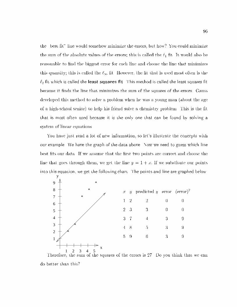
96
the \best �t" line would somehow minimize the errors, but how? You could minimize
the sum of the absolute values of the errors; this is called the `1 �t. It would also be
reasonable to �nd the biggest error for each line and choose the line that minimizes
this quantity; this is called the `1 �t. However, the �t that is used most often is the
`2 �t which is called the least squares �t. This method is called the least squares �t
because it �nds the line that minimizes the sum of the squares of the errors. Gauss
developed this method to solve a problem when he was a young man (about the age
of a high-school senior) to help his friend solve a chemistry problem. This is the �t
that is most often used because it is the only one that can be found by solving a
system of linear equations.
You have just read a lot of new information, so let's illustrate the concepts with
our example. We have the graph of the data above. Now we need to guess which line
best �ts our data. If we assume that the �rst two points are correct and choose the
line that goes through them, we get the line y = 1 + x: If we substitute our points
into this equation, we get the following chart. The points and line are graphed below.
1 2 3 4 5
1
2
3
4
5
6
7
8
9
*
*
*
*
*
x
y
x y predicted y error (error)2
1 2 2 0 0
2 3 3 0 0
3 7 4 3 9
4 8 5 3 9
5 9 6 3 9
Therefore, the sum of the squares of the errors is 27. Do you think that we can
do better than this?

97
If we choose the line that goes through the points when x = 3 and 4, we get the
line y = 4 + x: Will we get a better �t? Let's look at it.
1 2 3 4 5
1
2
3
4
5
6
7
8
9
*
*
*
*
*
x
y
x y predicted y error (error)2
1 2 5 �3 9
2 3 6 �3 9
3 7 7 0 0
4 8 8 0 0
5 9 9 0 0
The sum of the squares of the error is 18. That is a better �t, but can we do even
better?
Let's try the line that is half way between these two lines. The equation would
be y = 2:5 + x: It looks like this:
1 2 3 4 5
1
2
3
4
5
6
7
8
9
*
*
*
*
*
x
y
x y predicted y error (error)2
1 2 3:5 �1:5 2:25
2 3 4:5 �1:5 2:25
3 7 5:5 1:5 2:25
4 8 6:5 1:5 2:25
5 9 7:5 1:5 2:25
The sum of the squares of the error is 11.25 with this line, so this is the best line
yet. Can we do better? It doesn't seem very scienti�c or e�cient to keep guessing at

98
which line would give the best �t. Surely there is a methodical way to determine the
best �t line. Let's think about what we want.
A line in slope-intercept form looks like c0 + c1x = y where c0 is the y-intercept
and c1 is the slope. We want to �nd c0 and c1 such that c0 + c1xi = yi is true for all
our data points:
c0 + 1c1 = 2
c0 + 2c1 = 3
c0 + 3c1 = 7
c0 + 4c1 = 8
c0 + 5c1 = 9
We know that there may not exist c0 and c1 that �t all these equations, so we try to
�nd the best �t. We can write these equations in the form Xc = y (these are just
new letters for our familiar equation Ax = b) where
X =
266666666666664
1 1
1 2
1 3
1 4
1 5
377777777777775
; c =
264 c0
c1
375 ; and y =
266666666666664
2
3
7
8
9
377777777777775
:
In general, we cannot solve this system because the system is usually inconsistent
because it is overdetermined. In other words, we have more equations than unknowns
(the unknowns are the two variables, c0 and c1; for which we are trying to solve). There
is a system of equations called the normal equations that can be used to �nd least
squares solution to systems with more equations than unknowns.
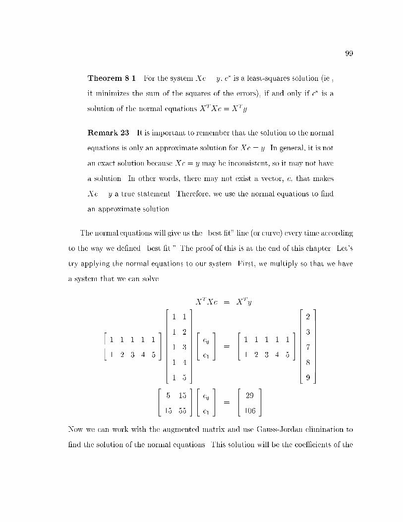
99
Theorem 8.1 For the system Xc = y, c� is a least-squares solution (ie.,
it minimizes the sum of the squares of the errors), if and only if c� is a
solution of the normal equations XTXc = X
Ty.
Remark 23 It is important to remember that the solution to the normal
equations is only an approximate solution for Xc = y. In general, it is not
an exact solution because Xc = y may be inconsistent, so it may not have
a solution. In other words, there may not exist a vector, c, that makes
Xc = y a true statement. Therefore, we use the normal equations to �nd
an approximate solution.
The normal equations will give us the \best �t" line (or curve) every time according
to the way we de�ned \best �t." The proof of this is at the end of this chapter. Let's
try applying the normal equations to our system. First, we multiply so that we have
a system that we can solve.
XTXc = X
Ty
264 1 1 1 1 1
1 2 3 4 5
375
266666666666664
1 1
1 2
1 3
1 4
1 5
377777777777775
264 c0
c1
375 =
264 1 1 1 1 1
1 2 3 4 5
375
266666666666664
2
3
7
8
9
377777777777775
264 5 15
15 55
375264 c0
c1
375 =
264 29
106
375
Now we can work with the augmented matrix and use Gauss-Jordan elimination to
�nd the solution of the normal equations. This solution will be the coe�cients of the

100
line which give the best �t in the least squares sense.
264 5 15
15 55
�������29
106
375 Augmented
System=)
264 1 3
15 55
�������5:8
106
375 r1� 5
264 1 3
0 10
�������5:8
19
375�15 � r1 + r2
=)
264 1 3
0 1
�������5:8
1:9
375r2� 10
264 1 0
0 1
�������0:1
1:9
375 �3 � r2 + r1
=)
264 c0
c1
375 =
264 0:1
1:9
375
When we graph and chart the line y = 0:1 + 1:9x, we get:
1 2 3 4 5
1
2
3
4
5
6
7
8
9
*
*
*
*
x
y
*
x y predicted y error (error)2
1 2 2:0 0 0
2 3 3:9 �:9 :81
3 7 5:8 1:2 1:44
4 8 7:7 :3 :09
5 9 9:6 �:6 :36
The sum of the squares of the error is 2.7. This is a great improvement over our
guesses and we know that we cannot do any better. In general, if we have n data
points, we solve XTXc = X
Ty with X =
266666666666664
1 x1
1 x2
......
1 xn�1
1 xn
377777777777775
, c =
264 c0
c1
375 and y =
266666666666664
y1
y2
...
yn�1
yn
377777777777775
:
The ellipse marks (written as...; � � � ; or
. . .) tell you to continue in the same pattern.

101
What if we are told that our data is not supposed to �t a straight line, but instead
falls in the shape of a parabola? Consider the following data from another experiment:
x y
-1 3
0 1
1 -1
2 1
3 31 2 3 4-1-2
-1
-2
1
2
3
4
*
*
*
**
We can �nd the curve that best �ts our data in a similar manner. The general
equation for a parabola is c0 + c1x+ c2x2 = y: Therefore, we want to �nd the values
of the coe�cients, c1; c2, and c3; so that the curve we �nd best �ts these equations:
c0 � 1c1 + 1c2 = 3
c0 + 0c1 + 0c2 = 1
c0 + 1c1 + 1c2 = �1
c0 + 2c1 + 4c2 = 1
c0 + 3c1 + 6c2 = 3

102
Let us use the normal equations with X =
266666666666664
1 �1 1
1 0 0
1 1 1
1 2 4
1 3 9
377777777777775
; c =
2666664
c0
c1
c2
3777775; and y =
266666666666664
3
1
�1
1
3
377777777777775
:
XTXc = X
Ty
2666664
1 1 1 1 1
�1 0 1 2 3
1 0 1 4 9
3777775
266666666666664
1 �1 1
1 0 0
1 1 1
1 2 4
1 3 9
377777777777775
2666664
c0
c1
c2
3777775
=
2666664
1 1 1 1 1
�1 0 1 2 3
1 0 1 4 9
3777775
266666666666664
3
1
�1
1
3
377777777777775
2666664
5 5 15
5 15 35
15 35 99
3777775
2666664
c0
c1
c2
3777775
=
2666664
7
7
33
3777775
Now we can augment the matrix and solve using Gaussian elimination.
2666664
5 5 15
5 15 35
15 35 99
�����������
7
7
33
3777775
Augmented
Matrix=)
2666664
1 1 3
5 15 35
15 35 99
�����������
125
7
33
3777775
r1� 5

103
2666664
1 1 3
0 10 20
0 20 54
�����������
125
0
12
3777775 �5 � r1 + r2
�15 � r1 + r3
=)
2666664
1 1 3
0 1 2
0 20 54
�����������
125
0
12
3777775 r2� 10
2666664
1 1 3
0 1 2
0 0 14
�����������
125
0
12
3777775�20 � r2 + r3
=)
2666664
1 1 3
0 1 2
0 0 1
�����������
125
0
67
3777775r3� 14
Back-substitution yields the coe�cients
c2 =67
c1 + 2�67
�= 0) c1 = �15
7
c0 +��15
7
�+ 3
�67
�= 12
5) c0 =
19352
666664
c0
c1
c2
3777775=
2666664
1935
�157
67
3777775
These coe�cients indicate that the curve we want is y = 1935� 15
7x+ 6
7x2: Let's graph
this curve and �ll in our chart:
1 2 3 4-1-2
-1
-2
1
2
3
4
*
*
*
**

104
x y expected y error (error)2
�1 3 3 435
�435
161225
0 1 1935
1635
2561225
1 �1 �1135
�2435
5761225
2 1 1935
1635
2561225
3 3 3 435
�435
161225
We �nd that the sum of the squared errors is 3235: Using our de�nition of least squares
\best �t," you will not be able to �nd a parabola that �ts the data better than this
one. In general, to �nd the parabola that best �ts the data, you use the normal
equations XTXc = X
Ty with
X =
266666666666664
1 x1 x21
1 x2 x22
......
...
1 xn�1 x2n�1
1 xn x2n
377777777777775
; c =
2666664
c0
c1
c2
3777775; and y =
266666666666664
y1
y2
...
yn�1
yn
377777777777775
:
Notice that the normal equations used to �nd the best �t line and the best �t
parabola have the same form. Do you think that we could expand this to higher degree
polynomials? Yes, we can. In general, we use the normal equations XTXc = X
Ty
with
X =
266666666666664
1 x1 x21 � � � x
m1
1 x2 x22 � � � x
m2
......
.... . .
...
1 xn�1 x2n�1 � � � x
mn�1
1 xn x2n � � � x
mn
377777777777775
; c =
266666666666664
c0
c1
...
cm�1
cm
377777777777775
; and y =
266666666666664
y1
y2
...
yn�1
yn
377777777777775
;
where m represents the degree of the polynomial curve that you wish to �t and n
represents the number of data points. The least squares \best �t" curve for these

105
equations is c0 + c1x + c2x2 + : : :+ cm�1x
m�1 + cmxm: Remember that the degree is
the highest power of the variable in your equation. A line is a �rst degree polynomial
and a parabola is a second degree polynomial.
If we can �nd the best �t curve for any degree polynomial, why don't we always
use a higher degree polynomial and �t the data better? After all, if we have n data
points and �t them to a polynomial of degree n � 1, we will have a perfect �t every
time because our systems would not be inconsistent. However, our goal is not just
to �nd a curve that �ts the data closely. Usually, we want the curve to predict what
would happen between our data points. If we choose a curve that exactly �ts all our
data points, we are incorporating the error in our measurements into our model unless
the model �ts the data exactly (which occurs only rarely.) Unfortunately, there is no
set rule for deciding what degree polynomial should be used to �t the data. However,
�rst and second degree polynomials provide the simplest models and should �t most
of your data until you start modeling more complicated systems.
If you notice, we said that we usually �t a curve so that we can predict what would
happen between our data points. Predicting an outcome between data points is called
interpolation. Why didn't we say anything about predicting the behavior beyond
our data points? Predicting an outcome beyond the data is called extrapolation.
It is usually dangerous to extrapolate much beyond the data because we have no
indication that the data will continue to follow the same curve since our curve was
only �t to the data. For example, we measured the height of a teenage boy every
year for a few years and charted his growth. The growth appeared linear, so we �t a
line to the data and got y = 32 + 2:25x. We have graphed the data with age on the
x-axis and height on the y-axis.

106
Age Height in inches
13 61:5
14 64:5
15 66:0
16 68:5
60
61
62
63
64
65
66
67
68
69
70
13 14 15 16 17
*
*
*
*
If we extrapolate back several years, this young man was over two and a half feet
tall when he was born. According to this model, he will never stop growing, so he
will be 8 feet 4 inches tall by the time he is 30 and almost 14 feet tall by the time he
is 60. Do you think that this is an accurate prediction?
If the temperature at the airport on the 4th of July was in the 90's for two years
in a row, would it be reasonable to predict that the temperature in January between
those years was also in the 90's? No, it would not. We have two problems with
this model. One problem is that we only have 2 data points. You can always �nd a
line that �ts the two points, but there is no reason to believe that the relationship
between the day of the year and the temperature is a linear relationship. Also, we
didn't take into account other factors that could a�ect our model such as the pattern
of the seasons. These are problems that can arise when you model a situation. When
we start modeling situations and using least squares to make predictions, we are
entering the world of statistics. That means that we must think about what the data
represents rather than just apply the normal equations. There are many interesting
applications of statistics that you can explore in another course. However, using
matrices, you already know one way to �nd a \best �t" curve for your data.

107
8.1 Proof of Normal Equations
We are interested in the fact that a solution to the normal equations is a least squares
solution. We will prove this fact, but will not prove the theorem in the other direction.
In this proof, y represents the solution of the normal equations (solution of ATAy =
ATb) and x is any n-vector.
The length of the vector x is de�ned to be kxk =qhx; xi =
qx21 + x
22 + : : :+ x
2n;
so the squared length of the vector is kxk2= hx; xi = x
Tx = x
21 + x
22 + � � � + x
2n:
The square of the length of the vector Ax� b, kAx� bk2, is the sum of the squares
of the errors since each element of Ax � b for data �tting represents the error at a
point. We want to prove that the sum of the squares of the error for y is less than
or equal to the sum of the squares of the error for x. In other words, we want to
prove that kAy � bk2� kAx� bk
2Notice that the steps of the proof are numbered.
Explanations for each step follow the proof.
To begin with; we have
0 � kAx� Ayk2
(1)
= (Ax� Ay)T(Ax� Ay) (2)
= (xTAT� y
TAT )(Ax� Ay) (3)
= xTATAx� x
TATAy � y
TATAx + y
TATAy: (4)
so
xTATAy + y
TATAx � x
TATAx+ y
TATAy (5)
equivalently;
2xTATAy � x
TATAx + y
TATAy (6)
Now; by adding and subtracting like terms; we obtain

108
2xTATAy � 2yTAT
Ay � 2xTATb + 2yTAT
b
� xTATAx+ y
TATAy � 2yTAT
Ay � 2xTATb + 2yTAT
b + bTb� b
Tb (7)
which we can rewrite as
2((xT � yT )(AT
Ay)� (xT � yT )(AT
b))
� (xTATAx� 2xTAT
b+ bTb)� (yTAT
A� 2yTATb + b
Tb) (8)
or
2(xT � yT )(AT
Ay � ATb) � (Ax� b)
T(Ax� b)� (Ay � b)
T(Ay � b): (9)
It follows that
0 � (Ax� b)T(Ax� b)� (Ay � b)
T(Ay � b): (10)
Hence
(Ay � b)T(Ay � b) � (Ax� b)
T(Ax� b) (11)
and
kAy � bk2� kAx� bk
2: (12)
1. This is the sum of numbers that have been squared. Squared numbers can not
be negative, so the sum of them can not be negative either.
2. kxk2= x
Tx
3. (M �N)T= M
T�N
T and (RS)T= S
TRT
4. Multiply binomials but remember that the order of multiplication matters.
FOIL is one method to multiply binomials.
5. Rearrange the terms
6. All the terms are 1 by 1 matrices, which we consider to be the same as real num-
bers. Transposing a real number does not change it. (xTATAy)
T= y
TATAx
109
7. We subtracted 2yTATAy and 2xTAT
b from both sides and added 2yTATb to
both sides of the inequality. Since we added and subtracted the same terms
from both sides of the inequality, we did not change the inequality. We also
added zero to the right-hand side of the inequality in the form of bT b � bTb.
We did all this so that we can factor to get what we want. This is similar to
completing the square.
8. Factor out the two from every term of the left-hand side. Then factor out
(xT � yT ) from the �rst two and last two terms of the left-hand side. On the
right-hand side, rearrange the terms.
9. On the left-hand side, factor out (xT �yT ). On the right-hand side, factor both
trinomials.
10. The left-hand side reduces to zero because ATAy = A
Tb.
11. Rearrange the inequality
12. xTx = kxk2
Question
So far, we have used the normal equations only to �t data to polynomials. Are
the normal equations restricted to polynomials?
Answer
No, the normal equations are not restricted to polynomials. They can be used
for any function of one variable. For example, we could �nd the curve that best �ts
the function y = c0 +c1xfor certain data points: We would solve XT
Xc = XTy with
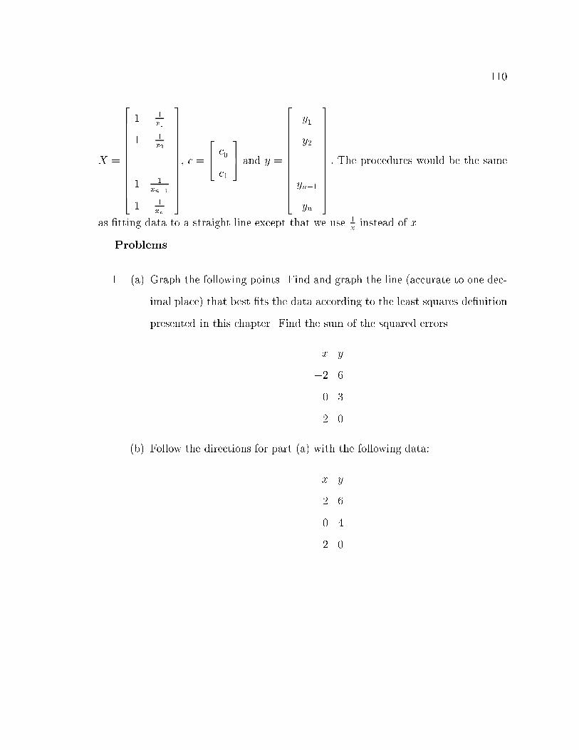
110
X =
266666666666664
1 1x1
1 1x2
......
1 1xn�1
1 1xn
377777777777775
, c =
264 c0
c1
375 and y =
266666666666664
y1
y2
...
yn�1
yn
377777777777775
: The procedures would be the same
as �tting data to a straight line except that we use 1xinstead of x.
Problems
1. (a) Graph the following points. Find and graph the line (accurate to one dec-
imal place) that best �ts the data according to the least squares de�nition
presented in this chapter. Find the sum of the squared errors.
x y
�2 6
0 3
2 0
(b) Follow the directions for part (a) with the following data:
x y
�2 6
0 4
2 0

111
(c) Follow the directions for part (a) with the following data:
x y
�2 6
�1 5
0 4
1 1
2 0
2. Find the line that best �ts this data:
x y
�2 8
0 6
1 5
2 3
3. Find the line that best �ts this data:
x y
1 3
3 10
4 11
6 19
8 24
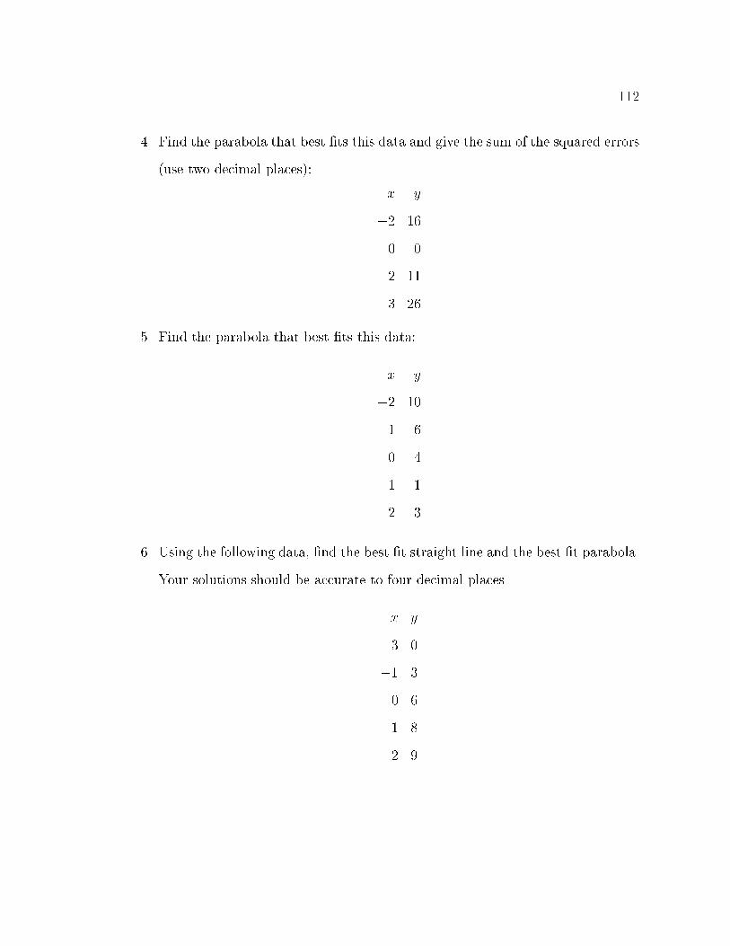
112
4. Find the parabola that best �ts this data and give the sum of the squared errors
(use two decimal places):
x y
�2 16
0 0
2 11
3 26
5. Find the parabola that best �ts this data:
x y
�2 10
�1 6
0 4
1 1
2 3
6. Using the following data, �nd the best �t straight line and the best �t parabola.
Your solutions should be accurate to four decimal places.
x y
�3 0
�1 3
0 6
1 8
2 9

113
7. Find the matrix X and the vector y that would be used in the normal equations
to �nd the best �t cubic (third degree) polynomial to the following data:
x y
�2 44
�1 11
0 3
1 1
3 �91
8. On a sunny day, measure the height of 5 objects and record those as x values.
Measure the shadows of your objects and record those as y values. It is best if
you take the measurements all at the same time and not around noon. Label
your data and graph it. Find the best �t line through the data.

114
Chapter 9
Eigenvalues and Eigenvectors
Have you ever heard the words eigenvalue and eigenvector? They are derived from the
German word \eigen" which means \proper" or \characteristic." An eigenvalue of a
square matrix is a scalar that is usually represented by the Greek letter � (pronounced
lambda). As you might suspect, an eigenvector is a vector. Moreover, we require that
an eigenvector be a non-zero vector, in other words, an eigenvector can not be the
zero vector. We will denote an eigenvector by the small letter x. All eigenvalues and
eigenvectors satisfy the equation Ax = �x for a given square matrix, A:
Remark 24 Remember that, in general, the word scalar is not restricted
to real numbers. We are only using real numbers as scalars in this book,
but eigenvalues are often complex numbers.
De�nition 9.1 Consider the square matrix A. We say that � is an
eigenvalue of A if there exists a non-zero vector x such that Ax = �x. In
this case, x is called an eigenvector (corresponding to �), and the pair
(�; x) is called an eigenpair for A.
Let's look at an example of an eigenvalue and eigenvector. If you were asked if x =264 1
�2
375 is an eigenvector corresponding to the eigenvalue � = 0 for A =
264 6 3
�2 �1
375,
you could �nd out by substituting x, �; and A into the equation Ax = �x:
Ax = �x264 6 3
�2 �1
375264 1
�2
375 = 0
264 1
�2
375
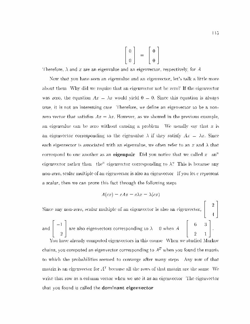
115
264 0
0
375 =
264 0
0
375
Therefore, � and x are an eigenvalue and an eigenvector, respectively, for A.
Now that you have seen an eigenvalue and an eigenvector, let's talk a little more
about them. Why did we require that an eigenvector not be zero? If the eigenvector
was zero, the equation Ax = �x would yield 0 = 0: Since this equation is always
true, it is not an interesting case. Therefore, we de�ne an eigenvector to be a non-
zero vector that satis�es Ax = �x: However, as we showed in the previous example,
an eigenvalue can be zero without causing a problem. We usually say that x is
an eigenvector corresponding to the eigenvalue � if they satisfy Ax = �x: Since
each eigenvector is associated with an eigenvalue, we often refer to an x and � that
correspond to one another as an eigenpair. Did you notice that we called x \an"
eigenvector rather than \the" eigenvector corresponding to �? This is because any
non-zero, scalar multiple of an eigenvector is also an eigenvector. If you let c represent
a scalar, then we can prove this fact through the following steps.
A(cx) = cAx = c�x = �(cx)
Since any non-zero, scalar multiple of an eigenvector is also an eigenvector,
264 2
�4
375
and
264 �1
2
375 are also eigenvectors corresponding to � = 0 when A =
264 6 3
�2 �1
375 :
You have already computed eigenvectors in this course. When we studied Markov
chains, you computed an eigenvector corresponding to AT when you found the matrix
to which the probabilities seemed to converge after many steps. Any row of that
matrix is an eigenvector for AT because all the rows of that matrix are the same. We
write that row as a column vector when we use it as an eigenvector. The eigenvector
that you found is called the dominant eigenvector
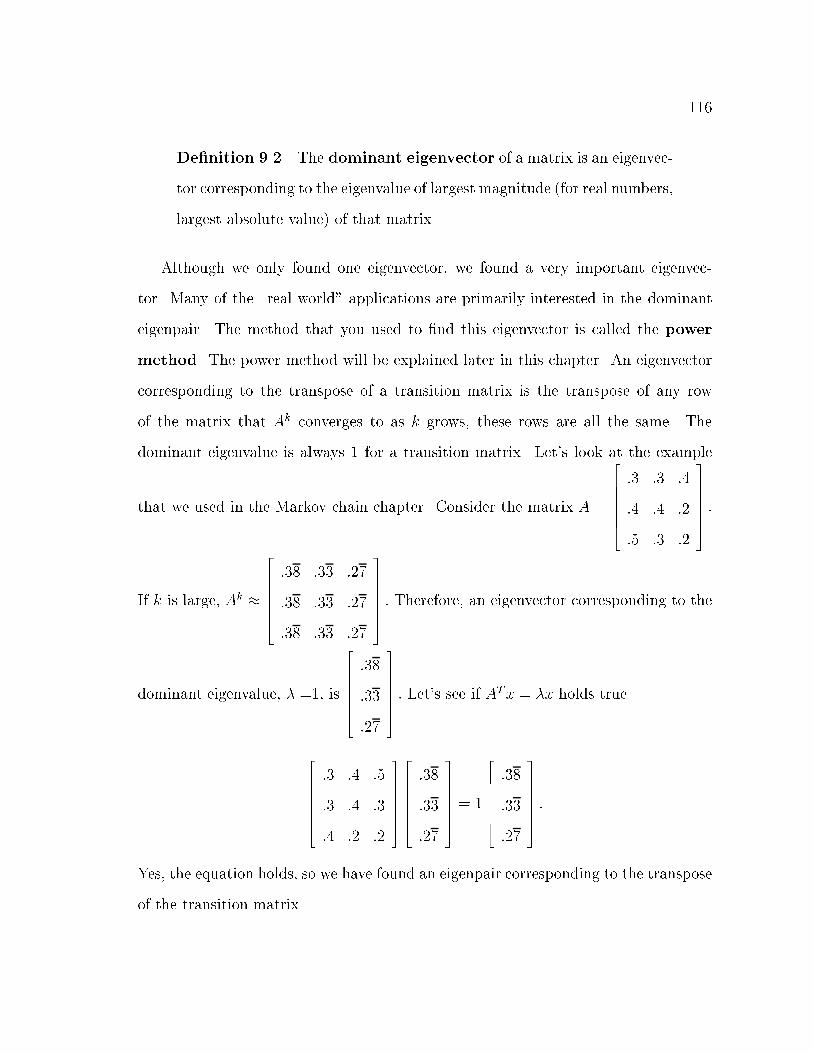
116
De�nition 9.2 The dominant eigenvector of a matrix is an eigenvec-
tor corresponding to the eigenvalue of largest magnitude (for real numbers,
largest absolute value) of that matrix.
Although we only found one eigenvector, we found a very important eigenvec-
tor. Many of the \real world" applications are primarily interested in the dominant
eigenpair. The method that you used to �nd this eigenvector is called the power
method. The power method will be explained later in this chapter. An eigenvector
corresponding to the transpose of a transition matrix is the transpose of any row
of the matrix that Ak converges to as k grows, these rows are all the same. The
dominant eigenvalue is always 1 for a transition matrix. Let's look at the example
that we used in the Markov chain chapter. Consider the matrix A =
2666664
:3 :3 :4
:4 :4 :2
:5 :3 :2
3777775:
If k is large, Ak�
2666664
:38 :33 :27
:38 :33 :27
:38 :33 :27
3777775: Therefore, an eigenvector corresponding to the
dominant eigenvalue, � =1, is
2666664
:38
:33
:27
3777775: Let's see if AT
x = �x holds true.
2666664
:3 :4 :5
:3 :4 :3
:4 :2 :2
3777775
2666664
:38
:33
:27
3777775= 1
2666664
:38
:33
:27
3777775:
Yes, the equation holds, so we have found an eigenpair corresponding to the transpose
of the transition matrix.
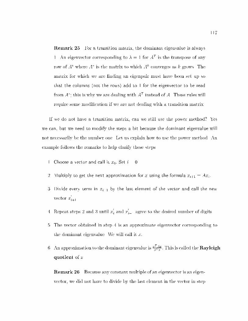
117
Remark 25 For a transition matrix, the dominant eigenvalue is always
1. An eigenvector corresponding to � = 1 for AT is the transpose of any
row of A� where A� is the matrix to which Ak converges as k grows. The
matrix for which we are �nding an eigenpair must have been set up so
that the columns (not the rows) add to 1 for the eigenvector to be read
from A�; this is why we are dealing with AT instead of A. These rules will
require some modi�cation if we are not dealing with a transition matrix.
If we do not have a transition matrix, can we still use the power method? Yes
we can, but we need to modify the steps a bit because the dominant eigenvalue will
not necessarily be the number one. Let us explain how to use the power method. An
example follows the remarks to help clarify these steps.
1. Choose a vector and call it x0: Set i = 0.
2. Multiply to get the next approximation for x using the formula xi+1 = Axi:
3. Divide every term in xi+1 by the last element of the vector and call the new
vector x0
i+1.
4. Repeat steps 2 and 3 until x0
i and x
0
i+1 agree to the desired number of digits.
5. The vector obtained in step 4 is an approximate eigenvector corresponding to
the dominant eigenvalue. We will call it x:
6. An approximation to the dominant eigenvalue is xTAxxTx
: This is called theRayleigh
quotient of x.
Remark 26 Because any constant multiple of an eigenvector is an eigen-
vector, we did not have to divide by the last element in the vector in step
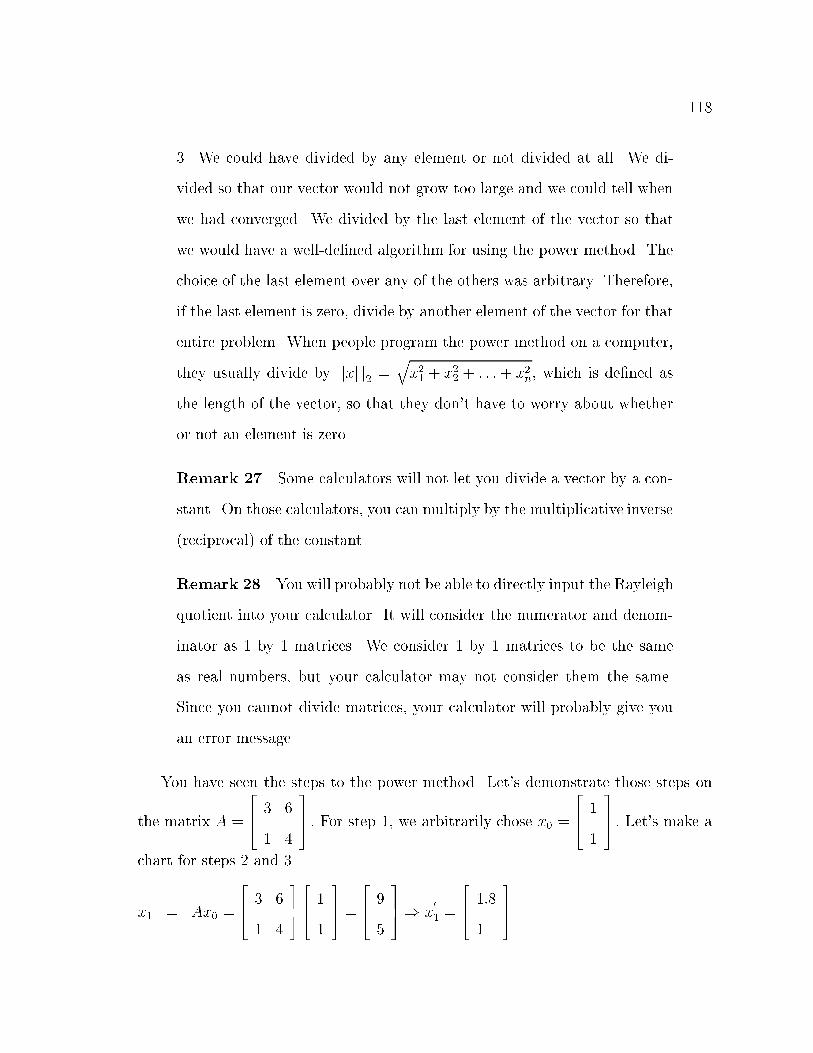
118
3. We could have divided by any element or not divided at all. We di-
vided so that our vector would not grow too large and we could tell when
we had converged. We divided by the last element of the vector so that
we would have a well-de�ned algorithm for using the power method. The
choice of the last element over any of the others was arbitrary. Therefore,
if the last element is zero, divide by another element of the vector for that
entire problem. When people program the power method on a computer,
they usually divide by jjxj j2 =qx21 + x
22 + : : :+ x
2n; which is de�ned as
the length of the vector, so that they don't have to worry about whether
or not an element is zero.
Remark 27 Some calculators will not let you divide a vector by a con-
stant. On those calculators, you can multiply by the multiplicative inverse
(reciprocal) of the constant.
Remark 28 You will probably not be able to directly input the Rayleigh
quotient into your calculator. It will consider the numerator and denom-
inator as 1 by 1 matrices. We consider 1 by 1 matrices to be the same
as real numbers, but your calculator may not consider them the same.
Since you cannot divide matrices, your calculator will probably give you
an error message.
You have seen the steps to the power method. Let's demonstrate those steps on
the matrix A =
264 3 6
1 4
375 : For step 1, we arbitrarily chose x0 =
264 1
1
375 : Let's make a
chart for steps 2 and 3.
x1 = Ax0 =
264 3 6
1 4
375264 1
1
375 =
264 9
5
375) x
0
1 =
264 1:8
1
375

119
x2 = Ax1 =
264 3 6
1 4
375264 1:8
1
375 =
264 11:4
5:8
375) x
0
2 =
264 1:965517241
1
375
x3 = Ax2 =
264 3 6
1 4
375264 1:965517241
1
375 =
264 11:89655172
5:96551724
375) x
0
3 =
264 1:994219653
1
375
x4 = Ax3 =
264 3 6
1 4
375264 1:994219653
1
375 =
264 11:98265896
5:99421965
375) x
0
4 =
264 1:99903568
1
375
Therefore, it looks like an eigenvector is x =
264 2
1
375 : The corresponding eigenvalue is:
xTAx
xTx
=
�2 1
� 264 3 6
1 4
375264 2
1
375
�2 1
� 264 2
1
375
=
�30
��5
� ) � = 6
Let's try to �nd the dominant eigenpair of another matrix. Consider the matrix
A =
264 2 6
2 �2
375 : Again, we will choose x0 =
264 1
1
375 ; but we could have chosen any
vector of dimension 2. Let's look at the chart for steps 2 and 3.
x1 =
264 2 6
2 �2
375264 1
1
375 =
264 8
0
375) x
0
1 =
264 1
0
375
We divided by 8 to get x0
1:We are allowed to do this because, as Remark 26 states, we
can divide by any element in the vector as long as we are consistent with our choice
throughout the problem.
x2 =
264 2 6
2 �2
375264 1
0
375 =
264 2
2
375) x
0
2 =
264 1
1
375
Notice that x
0
2 = x0. This means that our vectors will just continue in a cycle
and never converge. The power method only works if there is one eigenvalue whose

120
absolute value is strictly larger than the absolute value of the other eigenvalues. Even
when the power method works, convergence might be slow.
The power method found one very important eigenpair, but what should we do
if we want to �nd all the eigenpairs? We know that Ax = �x for all eigenpairs. We
can transform this equation into a form that will help us. When we learned about
the identity matrix, we learned that Ix = x for any x: Therefore, Ax = �Ix: We can
use algebra steps from here.
Ax = �Ix
Ax� �Ix = 0
(A� �I)x = 0
We know that x = 0 would solve this equation, but we de�ned an eigenvector to be
non-zero, so if there is an eigenvector solution to the equation (A � �I)x = 0; then
there must be more than one solution to the equation. We learned in Chapter 6 that
the system has a unique solution if det(A � �I) 6= 0: Therefore, we know that if
there is a non-zero solution to (A � �I)x = 0; then det(A � �I) = 0: The equation
det(A � �I) = 0 even has a name. It is called the characteristic equation. We
can solve the characteristic equation to �nd all the eigenvalues of certain matrices.
There will be as many eigenvalues as there are rows in the matrix (or columns since
the matrix must be square), but some of the eigenvalues might be identical to each
other.
Let's �nd both of the eigenvalues of the matrix A =
264 3 6
1 4
375 :
A� �I =
264 3� � 6
1 4� �
375
det(A� �I) = (3� �)(4� �)� 6

121
= �2� 7�+ 6
= (�� 6)(�� 1)
Therefore, � = 6 or � = 1: We now know our eigenvalues. Remember that all eigen-
values are paired with an eigenvector. Therefore, we can substitute our eigenvalues,
one at a time, into the formula (A � �I)x = 0 and solve to �nd a corresponding
eigenvector.
Let's �nd an eigenvector corresponding to � = 6:
(A� �I)x = 00B@264 3 6
1 4
375�
264 6 0
0 6
3751CAx =
264 0
0
375
264 �3 6
1 �2
375 x =
264 0
0
375
264 �3 6
1 �2
�������0
0
375 Augmented
Matrix264 1 �2
1 �2
�������0
0
375 r1� (�3)
264 1 �2
0 0
�������0
0
375�1 � r1 + r2
Notice that this system is underdetermined. Therefore, there are an in�nite number
of solutions. So, any vector that solves the equation x1 � 2x2 = 0 is an eigenvector
corresponding to � = 6 when A =
264 3 6
1 4
375 : To have a consistent method for �nding
an eigenvector, let's choose the solution in which x2 = 1. We can use back-substitution
to �nd that x1 � 2(1) = 0 which implies that x1 = 2. This tells us that
264 2
1
375 is an

122
eigenvector corresponding to � = 6 when A =
264 3 6
1 4
375 : This is the same solution
that we found when we used the power method to �nd the dominant eigenpair.
Let's �nd an eigenvector corresponding to � = 1:
(A� �I)x = 00B@264 3 6
1 4
375�
264 1 0
0 1
3751CAx =
264 0
0
375
264 2 6
1 3
375 x =
264 0
0
375
264 2 6
1 3
�������0
0
375 Augmented
Matrix264 1 3
1 3
�������0
0
375 r1� 2
264 1 3
0 0
�������0
0
375�1 � r1 + r2
Notice that this system is underdetermined. This will always be true when we are
�nding an eigenvector using this method. So, any vector that solves the equation
x1 + 3x2 = 0 is an eigenvector corresponding to the eigenvalue � = 1 when A =264 3 6
1 4
375 : Again, let's choose the eigenvector in which the last element of x is 1.
Therefore, x2 = 1 and x1 + 3(1) = 0; so x1 = �3: This tells us that
264 �3
1
375 is an
eigenvector corresponding to � = 1 when A =
264 3 6
1 4
375 : Using the characteristic

123
equation and Gaussian elimination, we are able to �nd all the eigenvalues to the
matrix and corresponding eigenvectors.
Let's �nd the eigenpairs for the matrix A =
264 2 6
2 �2
375 for which the power
method fails.
A� �I =
264 2� � 6
2 �2� �
375
det(A� �I) = (2� �)(�2� �)� 12
= �2� 16
= (�� 4)(�+ 4)
Therefore, � = 4 or � = �4: The power method does not work because j4j = j�4j :
In other words, there is not a unique dominant eigenvalue.
Let's �nd an eigenvector corresponding to � = 4:
(A� �I)x = 00B@264 2 6
2 �2
375�
264 4 0
0 4
3751CAx =
264 0
0
375
264 �2 6
2 �6
375 x =
264 0
0
375
264 �2 6
2 �6
�������0
0
375 Augmented
Matrix264 1 �3
2 �6
�������0
0
375 r1� (�2)
264 1 �3
0 0
�������0
0
375�2 � r1 + r2
124
Since the system is underdetermined, we have an in�nite number of solutions. Let's
choose the solution in which x2 = 1. We can use back-substitution to �nd that
x1 � 3(1) = 0 which implies that x1 = 3. This tells us that
264 3
1
375 is an eigenvector
corresponding to � = 4 when A =
264 2 6
2 �2
375 :
Let's �nd an eigenvector corresponding to � = �4:
(A� �I)x = 00B@264 2 6
2 �2
375�
264 �4 0
0 �4
3751CA x =
264 0
0
375
264 6 6
2 2
375 x =
264 0
0
375
264 6 6
2 2
�������0
0
375 Augmented
Matrix264 1 1
2 2
�������0
0
375 r1� 6
264 1 1
0 0
�������0
0
375�2 � r1 + r2
Again, let's choose the eigenvector in which the last element of x is 1. Therefore,
x2 = 1 and x1 + 1(1) = 0; so x1 = �1: This tells us that
264 �1
1
375 is an eigenvector
corresponding to � = �4 when A =
264 2 6
2 �2
375 : Using the characteristic equation
and Gaussian elimination, we are able to �nd both of the eigenvalues to the matrix
and corresponding eigenvectors.

125
We can �nd eigenpairs for larger systems using this method, but the characteristic
equation gets impossible to solve directly when the system gets too large. We could
use approximations that get close to solving the characteristic equation, but there are
better ways to �nd eigenpairs that you will study in the future. However, these two
methods give you an idea of how to �nd eigenpairs.
Another matrix for which the power method will not work is the matrix A =264 5 0
0 5
375 ; because the eigenvalues are both the real number 5. The method that we
showed you earlier will yield the eigenvector
264 0
1
375 to correspond to the eigenvalue
� = 5. Other methods will reveal, and you can check, that
264 1
0
375 is also an eigenvector
of A corresponding to � = 5. Notice that these two eigenvectors are not multiples of
one another. If the same eigenvalue is repeated p times for a particular matrix, then
there can be as many as p di�erent eigenvectors that are not multiples of each other
that correspond to that eigenvalue.
We said that eigenvalues are often complex numbers. However, if the matrix A
is symmetric, then the eigenvalues will always be real numbers. As you can see from
the problems that we worked, eigenvalues can also be real when the matrix is not
symmetric, but keep in mind that they are not guaranteed to be real.
Did you know that the determinant of a matrix is related to the eigenvalues of the
matrix? The product of the eigenvalues of a square matrix is equal to the determinant
of that matrix. Let's look at the two matrices that we have been working with. For
A =
264 3 6
1 4
375 ;
Product of eigenvalues = det(A)
126
6 � 1 = 12� 6
6 = 6
For A =
264 2 6
2 �2
375 ;
Product of eigenvalues = det(A)
4 � (�4) = �4� 12
�16 = �16
You can use this as a check to see that you have the correct eigenvalues and deter-
minant for the matrix A:
Now that we know how to �nd eigenpairs, we might want to know what uses
they have. The interesting uses come from larger systems, so we will just discuss
them rather than solve them. Have you ever seen the video of the collapse of the
Tacoma Narrows Bridge? The Tacoma Bridge was built in 1940. From the begin-
ning, the bridge would form small waves like the surface of a body of water. This
accidental behavior of the bridge brought many people who wanted to drive over this
moving bridge. Most people thought that the bridge was safe despite the movement.
However, about four months later, the oscillations (waves) became bigger. At one
point, one edge of the road was 28 feet higher than the other edge. Finally, this
bridge crashed into the water below. One explanation for the crash is that the oscil-
lations of the bridge were caused by the frequency of the wind being too close to the
natural frequency of the bridge. The natural frequency of the bridge is the eigenvalue
of smallest magnitude of a system that models the bridge. This is why eigenvalues
are very important to engineers when they analyze structures. (Di�erential Equations
and Their Applications, 1983, pp. 171-173).

127
Remark 29 The eigenvalue of smallest magnitude of a matrix is the
same as the inverse (reciprocal) of the dominant eigenvalue of the inverse
of the matrix. Since most applications of eigenvalues need the eigenvalue
of smallest magnitude, the inverse matrix is often solved for its dominant
eigenvalue. This is why the dominant eigenvalue is so important.
Also, a bridge in Manchester, England collapsed in 1831 because of con icts
between frequencies. However, this time, the natural frequency of the bridge was
matched by the frequency caused by soldiers marching in step. Large oscillations
occurred and the bridge collapsed. This is why soldiers break cadence when crossing
a bridge.
Frequencies are also used in electrical systems. When you tune your radio, you are
changing the resonant frequency until it matches the frequency at which your station
is broadcasting. Engineers used eigenvalues when they designed your radio.
Frequencies are also vital in music performance. When instruments are tuned,
their frequencies are matched. It is the frequency that determines what we hear as
music. Although musicians do not study eigenvalues in order to play their instruments
better, the study of eigenvalues can explain why certain sounds are pleasant to the
ear while others sound \ at" or \sharp." When two people sing in harmony, the
frequency of one voice is a constant multiple of the other. That is what makes the
sounds pleasant. Eigenvalues can be used to explain many aspects of music from the
initial design of the instrument to tuning and harmony during a performance. Even
the concert halls are analyzed so that every seat in the theater receives a high quality
sound.
Car designers analyze eigenvalues in order to damp out the noise so that the
occupants have a quiet ride. Eigenvalue analysis is also used in the design of car
stereo systems so that the sounds are directed correctly for the listening pleasure of
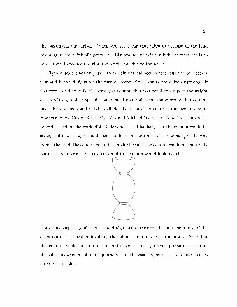
128
the passengers and driver. When you see a car that vibrates because of the loud
booming music, think of eigenvalues. Eigenvalue analysis can indicate what needs to
be changed to reduce the vibration of the car due to the music.
Eigenvalues are not only used to explain natural occurrences, but also to discover
new and better designs for the future. Some of the results are quite surprising. If
you were asked to build the strongest column that you could to support the weight
of a roof using only a speci�ed amount of material, what shape would that column
take? Most of us would build a cylinder like most other columns that we have seen.
However, Steve Cox of Rice University and Michael Overton of New York University
proved, based on the work of J. Keller and I. Tadjbakhsh, that the column would be
stronger if it was largest at the top, middle, and bottom. At the points 14of the way
from either end, the column could be smaller because the column would not naturally
buckle there anyway. A cross-section of this column would look like this:
Does that surprise you? This new design was discovered through the study of the
eigenvalues of the system involving the column and the weight from above. Note that
this column would not be the strongest design if any signi�cant pressure came from
the side, but when a column supports a roof, the vast majority of the pressure comes
directly from above.

129
Eigenvalues can also be used to test for cracks or deformities in a solid. Can
you imagine if every inch of every beam used in construction had to be tested?
The problem is not as time consuming when eigenvalues are used. When a beam
is struck, its natural frequencies (eigenvalues) can be heard. If the beam \rings,"
then it is not awed. A dull sound will result from a awed beam because the aw
causes the eigenvalues to change. Sensitive machines can be used to \see" and \hear"
eigenvalues more precisely.
Oil companies frequently use eigenvalue analysis to explore land for oil. Oil, dirt,
and other substances all give rise to linear systems which have di�erent eigenvalues,
so eigenvalue analysis can give a good indication of where oil reserves are located.
Oil companies place probes around a site to pick up the waves that result from a
huge truck used to vibrate the ground. The waves are changed as they pass through
the di�erent substances in the ground. The analysis of these waves directs the oil
companies to possible drilling sites.
There are many more uses for eigenvalues, but we only wanted to give you a
sampling of their uses. When you study science or engineering in college, you will
become quite familiar with eigenvalues and their uses. There are also numerical
di�culties that can arise when data from real-world problems are used. Some of
these di�culties are discussed in Chapter 10.

130
Problems
1. Use the power method to �nd the dominant eigenpair for the transpose of the
matrix A =
2666664
:2 :3 :5
:4 :4 :2
:4 :6 0
3777775which was used in problem 6 of Chapter 7. Give
your solution accurate to two decimal places.
2. Use the power method to �nd the dominant eigenpair for the transpose of the
matrix A =
2666664
:4 :35 :25
:45 :4 :15
:8 :15 :05
3777775which was used in problem 7 of Chapter 7. Give
your solution accurate to two decimal places.
3. Use the power method to �nd the dominant eigenpair for A =
264 1 0
4 8
375 :
4. Use the power method to �nd the dominant eigenpair for A =
264 3 2:5
1 1:5
375 :
5. Use the characteristic equation to �nd all the eigenvalues of A =
264 3 5
1 �1
375
and a corresponding eigenvector for each.
6. Use the characteristic equation to �nd all the eigenvalues of A =
264 5 0
2 �2
375
and a corresponding eigenvector for each.
7. Use the characteristic equation to �nd all the eigenvalues of A =
264 3 7
2 �2
375
and a corresponding eigenvector for each.
131
8. If
26666666664
�3
2
�1
1
37777777775is an eigenvector corresponding to � = 5; �nd 3 more eigenvectors
that correspond to � = 5:

132
Chapter 10
Numerical Challenges
Since you have successfully worked so many problems with matrices, you may be
wondering why people still need to study them. The methods for dealing with ma-
trices that you have learned work nicely for most small matrices, but di�culties are
encountered when the matrices are larger. Can you imagine solving by hand a system
of equations in which A was of dimension 10 by 10? That would take a dreadfully
long time. However, a computer can solve this system quickly. Does that mean that
a computer can solve all systems? What if the system involved a matrix with dimen-
sions of 100,000 by 100,000? The computer could have di�culty with this system.
You might be thinking that this is a ridiculous size for a system of equations, but
systems this size and larger are needed in most industrial applications. For example,
the major airlines need systems of this size to schedule ights and crews. Also, large
systems are needed when an oil or water reservoir is simulated to learn about how to
best pump the liquid or perform an environmental cleanup.
One problem is that the system might be too large for the computer's memory
to hold all the information at one time. This means that new algorithms must be
found that require less of the problem to be stored in memory at one time. These
new algorithms still need to arrive at the correct solution in a reasonable amount of
time.
The amount of work (the number of individual additions, subtractions, multipli-
cations, or divisions) needed to solve a system also depends on the size of the system
(among other properties such as the percentage of zeros in the matrix and where the
non-zero numbers are in the matrix). Even if the computer can solve this system,

133
will it be able to do it in a reasonable amount of time? In many ways, Gaussian
elimination is our method of choice for solving linear systems. Yet, even Gaussian
elimination may take days, months, or even years to solve very large linear systems
on the world's fastest computers. Researchers are working to �nd algorithms that will
solve systems with less work. They are also working in the �eld of parallel computing
in which the problem is broken down into parts. Parts that do not depend on one
another can be sent to separate processing units so that those parts of the problem
can be processed at the same time. Computers are already extremely fast, so the
room that is left for improvement lies mostly in improving algorithms. There are also
many problems that still cannot be solved. These are reasons why researchers are
needed in the mathematical sciences.
Roundo� error is probably the biggest detriment to e�ective computation because
it can a�ect small problems as well as large ones. If you try to turn the fraction 13
into a decimal, you can carry out the approximation as far as you want. However, a
computer has only a set number of digits that it can store for each number. Therefore,
the fraction 13has to be rounded at some point. For a single number, this rounding
is not too signi�cant, but it becomes important when operations are performed with
rounded numbers. Most computers store numbers in a manner similar to scienti�c
notation called normal notation. In normal notation, a number is written as m� 10a
where 0:1 � jmj < 1. (In scienti�c notation, 1 � jmj < 10). In this equation, m
stands for mantissa and a stands for abscissa. The number 1234 is represented as
0.1234� 104. (Since most computers work in the binary system rather than the dec-
imal system, this is not entirely accurate, but it will su�ce to demonstrate roundo�
error). The mantissa of this example is 0.1234. The abscissa is 4. For demonstration
purposes, let us pretend that our computer stores 4-digit mantissas and 2-digit ab-
134
scissas (the sign of the number is not included in the 4 digits of the mantissa on our
�ctional computer).
Let's add 10 + :00001: The exact arithmetic solution is 10:00001: Our computer
stores this as 0:1000� 102+0:1000� 10�4: When added, this yields 0:1000001� 102:
However, our computer will only store a 4 digit mantissa, so this rounds to 0:1000�102
which is the �rst addend of our problem. This means that our solution does not re ect
that we added 0:1000� 10�4 at all. Our solution is only o� by 0:1000� 10�4 which
may not be much, but suppose that we want to add the number 0:1000 � 10�4 ten
thousand times to the number 10 rather than just once. The exact solution is 11, but
our computer still gives the solution as 10 because each time that we add 0:1000�10�4
to our solution, it doesn't make a di�erence. The source of this problem is that the
two numbers that we are adding are of such di�erent magnitudes. We can correct
this problem by summing 0:1000� 10�4 ten thousand times before we add the result
to 10. This will yield a much closer solution. Roundo� problems can be minimized
by paying attention to details like the order of magnitude of the numbers, but they
cannot be eliminated.
Subtractive cancellation is another big problem when dealing with computers.
When you subtract two numbers that are very close to each other, an error is in-
troduced. Suppose we want to perform this operation on our �ctional computer:
0:5555� 0:5554: Of course, the accurate solution is 0.0001, but that is not necessarily
what the computer obtains. The computer represents this as 0:5555� 100� 0:5554�
100. The subtraction yields 0:0001 � 100, but the computer stores this number in
normal form, so it should be stored as 0:1 � 10�3: However, the computer �lls all 4
digits of the mantissa. Since there is no accurate information for the other 3 digits
of the mantissa, some computers �ll the slots with random digits rather than zeros.
Therefore, the solution is stored as 0:1ddd� 10�3, where the d's are random digits.
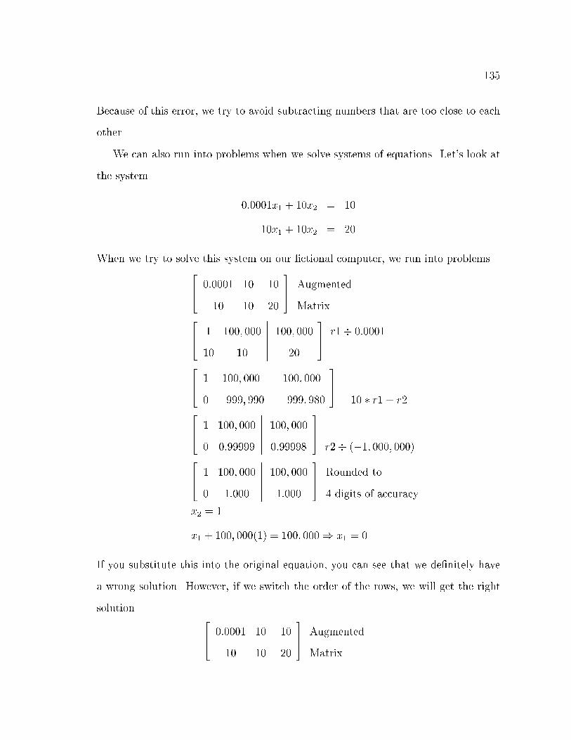
135
Because of this error, we try to avoid subtracting numbers that are too close to each
other.
We can also run into problems when we solve systems of equations. Let's look at
the system
0:0001x1 + 10x2 = 10
10x1 + 10x2 = 20
When we try to solve this system on our �ctional computer, we run into problems.264 0:0001 10
10 10
�������10
20
375 Augmented
Matrix264 1 100; 000
10 10
�������100; 000
20
375 r1� 0:0001
264 1 100; 000
0 �999; 990
�������100; 000
�999; 980
375�10 � r1 + r2
264 1 100; 000
0 0:99999
�������100; 000
0:99998
375r2� (�1; 000; 000)
264 1 100; 000
0 1:000
�������100; 000
1:000
375 Rounded to
4 digits of accuracy
x2 = 1
x1 + 100; 000(1) = 100; 000) x1 = 0
If you substitute this into the original equation, you can see that we de�nitely have
a wrong solution. However, if we switch the order of the rows, we will get the right
solution. 264 0:0001 10
10 10
�������10
20
375 Augmented
Matrix
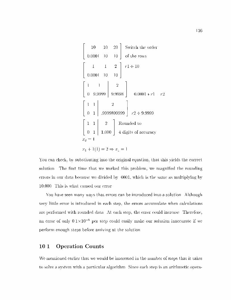
136
264 10 10
0:0001 10
�������20
10
375 Switch the order
of the rows264 1 1
0:0001 10
�������2
10
375 r1� 10
264 1 1
0 9:9999
�������2
9:9998
375�0:0001 � r1 + r2
264 1 1
0 1
�������2
:9999899999
375r2� 9:9999
264 1 1
0 1
�������2
1:000
375 Rounded to
4 digits of accuracy
x2 = 1
x1 + 1(1) = 2) x1 = 1
You can check, by substituting into the original equation, that this yields the correct
solution. The �rst time that we worked this problem, we magni�ed the rounding
errors in our data because we divided by .0001, which is the same as multiplying by
10,000. This is what caused our error.
You have seen many ways that errors can be introduced into a solution. Although
very little error is introduced in each step, the errors accumulate when calculations
are performed with rounded data. At each step, the error could increase. Therefore,
an error of only 0.1�10�6 per step could easily make our solution inaccurate if we
perform enough steps before arriving at the solution.
10.1 Operation Counts
We mentioned earlier that we would be interested in the number of steps that it takes
to solve a system with a particular algorithm. Since each step is an arithmetic opera-

137
tion, when we count the steps, we are counting the operations. Addition/subtraction
steps are a lot quicker to compute than multiplication/division steps. Also, there are
usually approximately the same number of addition/subtraction steps as multiplica-
tion/division steps in an algorithm. Therefore, since operation counts are only an
approximation, we will only consider the multiplication/division steps.
We told you that Gaussian elimination requires fewer steps than Gauss-Jordan
elimination, so we would like to show you how big of a di�erence that can make.
Gaussian elimination requires approximately n3
3+n2
�n
3multiplication/division steps.
Gauss-Jordan requires approximately n3
2+n2
2multiplication/division steps (Elementary
Linear Algebra, 1974, p. 38-39). Let's compute the approximate number of multi-
plcation steps needed for several values of n.
n Gauss Gauss� Jordan
2 6 6
3 17 18
4 36 40
5 65 75
6 106 126
10 430 550
100 343; 300 505; 000
1000 334; 333; 000 500; 500; 000
large n n3
3n3
2
The last line indicates an approximation for large n because the terms that have
powers less than 3 are small compared to the third order term. For small systems,
the two methods do not di�er much, but the di�erence is drastic for large systems.
We could also look at the e�ciency of Cramer's rule, but it depends on how we
compute the determinant. We must compute n+ 1 determinants, but the method of

138
computation makes a di�erence. The computation of the determinant for an n by n
matrix using expansion by minors requires n! multiplications/divisions because there
are n minors required for the �rst expansion and each submatrix needed to determine
the minor must also be expanded in the same manner until the submatrices are 3 by 3
or smaller. If we use expansion by minors to compute the determinant, then Cramer's
rule requires approximately (n + 1)! multiplications/divisions. If we compute the de-
terminant using Gaussian elimination, then Cramer's rule requires approximately n4
3
multiplications/divisions because Gaussian elimination for each determinant requires
approximately n3
3multiplications/divisions and n+ 1 determinants are needed. This
is why we said that Cramer's rule is a theoretical tool, not a computational tool.
Let's look at the number of multiplications/divisions required for several values of n
for each method.
n Expansion by Minors Using Gaussian Elimination
2 2 6
3 6 27
4 24 86
5 120 208
6 720 432
10 518; 400 3334
50 3 � 1064 2; 083; 333
Factorials grow so quickly, that our calculators will not even store enough digits to
compute the number of operations needed to use expansion by minors in Cramer's
rule for n = 100:We certainly don't want to use an algorithm that requires that many
operations when we have better options.
Although this chapter presents many problems that can occur when solving sys-
tems or using computers, it was not intended to discourage you. The methods that

139
you learned in the previous chapters will work for most matrices that are not too
large. However, you do need to be aware of some of the pitfalls of calculations so
that you can avoid them. These problems are part of the reason for the national need
for researchers in the �eld of computational mathematics. Hopefully, your eyes have
been opened to an exciting possible career.

140
Second Review
1. A school district has 3 high schools. At the end of each year, teachers can be
moved from one school to another. The picture below depicts the probability
that a teacher will move from one school to another this year.
A C
B
.6 .7
.6
.3 .2.2 .1
.1
.2
(a) Construct and label the transition matrix that corresponds to this picture.
Name the matrix A:
(b) If a teacher works in school A this year, what is the probability that he or
she will work in school C next year?
(c) If a teacher works in school C this year, what is the probability that he or
she will work in school B in the year after next (i.e., 2 years from now)?
(d) Matrix A is the transition matrix for one year. Find the transition matrix
for two years.
(e) Find the transition matrix for three years.
(f) Find, to two decimal places, the matrix to which A appears to converge
after many years.
(g) Explain the meaning of your solution to problem 1f.

141
2. (a) Using the following data and the normal equation, �nd the \best �t"
straight line, accurate to one decimal place, to the points.
x y
1 3
2 5
4 10
5 13
7 14
(b) Using the following data and the normal equation, �nd the \best �t"
straight line, accurate to one decimal place, to the points.
x y
�1 �4
1 1
2 4
3 7
4 11
3. (a) Using the following data and the normal equation, �nd the \best �t"
parabola, accurate to one decimal place, to the points.
x y
�3 8
�1 �3
0 �1
2 13
4 40
142
(b) Using the following data and the normal equation, �nd the \best �t"
parabola, accurate to one decimal place, to the points.
x y
�2 18
�1 6
0 0
2 10
4 40
4. (a) Use the power method to �nd the dominant eigenpair of the matrix A from
problem 1.
(b) Use the power method to �nd the dominant eigenpair of the matrix264 5 �6
�2 1
375 :
(c) Use the characteristic equation to �nd both of the eigenpairs of the matrix264 2 �4
1 �3
375 :

143
Matrix Test 1A
1. On average, Heather spends 3 hours on homework, 4 hours watching TV, and
8 hours sleeping each day. Reena watches 1 hour of TV, sleeps 6 hours, and
spends 5 hours doing homework. Edwin works on homework for an hour and
sleeps for 9 hours. Mark sleeps 7 hours a day, watches 3 hours of TV, and
spends 2 hours on homework.
(a) Put the information into a 4 by 3 matrix and label it.
(b) Transpose the matrix from problem 1a and attach labels.
(c) If Edwin spends 5 hours a day with his computer and no one else works on
a computer daily, convert the matrix from problem 1a into a 4 by 4 matrix
and attach labels.
2. What is the sum
264 4 �1
7 2
375 +
264 �6 5
�3 �1
375?
3. What is the product
264 3 �7
4 9
375264 5 �6
4 2
375?
4. Find the inverse of the matrix
264 4 6
1 2
375
5. Give the two major steps needed to �nd the inverse of this matrix
2666664
3 4 1
1 2 1
�2 2 3
3777775
OR actually �nd the inverse. (Only answer one of the questions. Both questions
are worth the same number of points, so it doesn't matter which you answer).

144
6. Construct a symmetric matrix and explain why it is symmetric.
7. Solve this system using Gaussian elimination or Gauss-Jordan elimination and
tell which method you used.
2x1 + x2 + 3x3 = 11
4x1 � x2 + 2x3 = 5
3x2 + 2x3 = 13
8. Find the determinant of the matrix
26666666664
7 2 5 3
1 0 2 0
8 0 �2 4
�3 0 4 1
37777777775:
9. Label each of these systems as consistent or inconsistent. If the system is
consistent, further categorize it as underdetermined or uniquely determined.
Explain why each system is categorized as it is.
(a) Ax = b where A =
264 2 1
3 �2
375 and b =
264 10
1
375
(b) 3x1 + 4:5x2 = 6
2x1 + 3x2 = 4

145
Matrix Test 1B
1. On average, Gail spends 3 hours a day at her job, 2 hours studying, an hour
watching TV, and 8 hours sleeping. Kerry spends 2 hours watching TV, 3 hours
studying, 2 hours working, and 7 hours sleeping. Brad spends 5 hours a day
working, 4 hours studying, and 6 hours sleeping.
(a) Put the information into a 3 by 4 matrix and label it.
(b) Transpose the matrix from problem 1a and attach labels.
(c) Adam works 12 hours a day and sleeps 7 hours. Convert the matrix from
problem 1a into a 4 by 4 matrix and attach labels.
2. What is the sum
264 2 5
6 �1
375 +
264 2 4
3 4
375?
3. What is the product
264 2 �5
3 8
375264 7 �4
0 5
375?
4. Find the inverse of the matrix
264 5 4
�2 �1
375 :
5. Give the two major steps needed to �nd the inverse of this matrix
2666664
1 2 1
3 �1 2
1 3 1
3777775
OR actually �nd the inverse. (Only answer one of the questions. Both questions
are worth the same number of points, so it doesn't matter which you answer).
6. Construct a symmetric matrix and explain why it is symmetric.
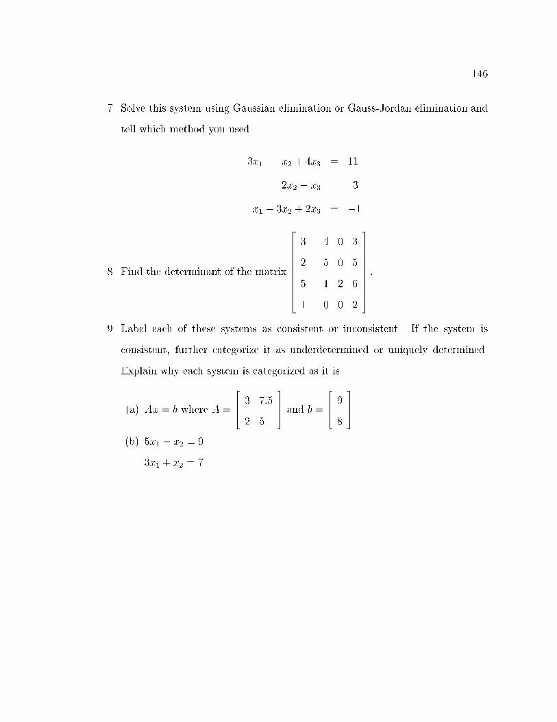
146
7. Solve this system using Gaussian elimination or Gauss-Jordan elimination and
tell which method you used.
3x1 � x2 + 4x3 = 11
2x2 � x3 = 3
x1 � 3x2 + 2x3 = �1
8. Find the determinant of the matrix
26666666664
3 �4 0 3
2 5 0 5
5 1 2 6
1 0 0 2
37777777775:
9. Label each of these systems as consistent or inconsistent. If the system is
consistent, further categorize it as underdetermined or uniquely determined.
Explain why each system is categorized as it is.
(a) Ax = b where A =
264 3 7:5
2 5
375 and b =
264 9
8
375
(b) 5x1 � x2 = 9
3x1 + x2 = 7

147
Matrix Test 1C
1. Complete the following using matrices. When you create a matrix, label it. If a
matrix does not clearly answer the question, please write a sentence to explain
your answer.
Shelly and Clint make dog houses. They call their company Canine Cabins.
Shelly builds the walls. Clint builds the roof and oor. Then Clint attaches
the roof and oor to the walls and Shelly paints it. Canine Cabins come in two
sizes. The walls of a small house require 25 square feet of wood and 1 hour of
labor. The roof and oor require 15 square feet of wood and an hour of labor.
The walls of a large house require 70 square feet of wood and an hour of labor.
The roof and oor of a large house use 30 square feet of wood and an hour of
labor.
(a) Compile this information into two 2 by 3 matrices (remember that we have
not used paint yet, but we will). You will have one matrix for walls and
one for roof and oor.
(b) Using the matrices, determine how much wood, paint, and labor are used
for each house before they are assembled if we build one large and one
small house.
(c) A completed small houses requires 40 square feet of wood, 1 pint of paint,
and 3.5 hours of labor. A large house requires 100 square feet of wood, 1.5
pints of paint, and 4 hours labor. Form the 2 by 3 matrix that represents
the total units of each material required to complete each size of house.
148
(d) Determine how much wood, paint, and time are required to attach the roof
and oor to the walls and paint the house for each size.
(e) If wood costs $0.50 per square foot, paint costs $6 per pint, and Shelly and
Clint earn $8 per hour, how much does each size house cost to produce?
(f) This month, Canine Cabins had orders for 30 small houses and 20 large
houses. How much of each material do they need to �ll the orders?
(g) How much money will they need to buy the material to �ll the orders?
2. If A is a 3 by 4 matrix, B is 2 by 4, and C is 2 by 3, list all the ways using (A
or AT ), (B or BT ), and (C or CT ) that you can multiply these three matrices
together. Each matrix or its transpose must be used exactly once in each
multiplication.
3. Given
A =
2666664
1 2 1
3 �1 2
3 1 2
3777775and b =
2666664
2
11
9
3777775
(a) Find the determinate of A.
(b) Solve the system Ax = b using Gaussian elimination or Gauss-Jordan
elimination. Specify which you are using.
(c) Find the inverse of A.
(d) How would you prove that your solution to problem 3c is actually the
inverse of A?
4. Create a matrix for which an inverse does not exist and explain why an inverse
does not exist.

149
5. Create a system for each of the following descriptions and explain why the
system �ts the description.
(a) Consistent and underdetermined
(b) Consistent and uniquely determined
(c) Inconsistent

150
Matrix Test 2A
1. An amateur meteorologist predicts the weather based solely on today's weather.
The picture below depicts the probability that the weather will either be sunny,
cloudy, or rainy based on the weather today.
S
C
R
.5 .3
.2
.3 .5.3 .4
.2
.3
(a) Construct and label the transition matrix that corresponds to this picture.
Name the matrix A:
(b) If the weather is rainy today, what is the probability that it will be cloudy
tomorrow?
(c) If it is sunny today, what is the probability that it will be cloudy the day
after tomorrow (ie., 2 days from now)?
(d) Matrix A is the transition matrix for one day. Find the transition matrix
for two days.
(e) Find the transition matrix for three days.
(f) Find, to three decimal places, the matrix to which A appears to converges
after many days.
(g) Explain the meaning of your solution to problem 1f.
151
2. Using the following data and the normal equation, �nd the \best �t" straight
line, accurate to one decimal place, to the points.
x y
�2 4
0 1
1 0
2 3
3. Using the following data and the normal equation, �nd the \best �t" parabola,
accurate to one decimal place, to the points.
x y
�2 �4
0 5
1 0
2 �12
4. (a) Use the power method to �nd the dominant eigenpair of the matrix A from
problem 1.
(b) Use the power method to �nd the dominant eigenpair of the matrix264 �6 2
�3 1
375 :
(c) Use the characteristic equation to �nd both of the eigenpairs of the matrix264 �2 �9
�2 1
375 :
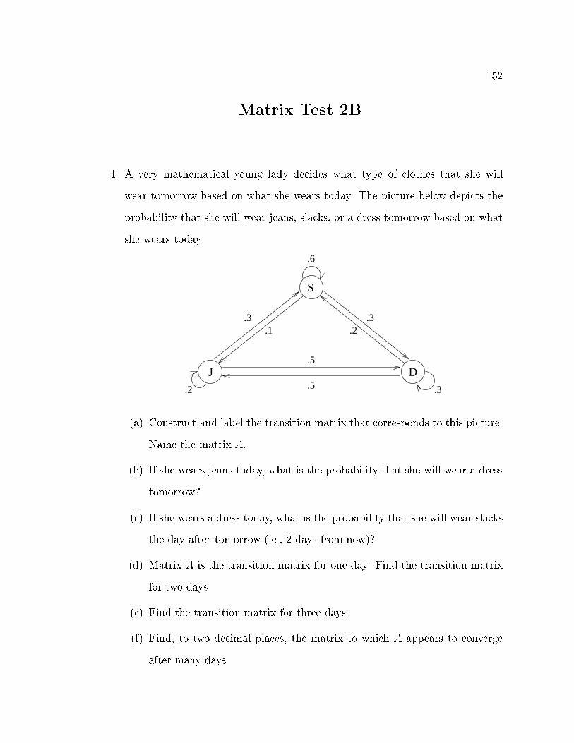
152
Matrix Test 2B
1. A very mathematical young lady decides what type of clothes that she will
wear tomorrow based on what she wears today. The picture below depicts the
probability that she will wear jeans, slacks, or a dress tomorrow based on what
she wears today.
S
DJ
.2
.6
.3
.5
.5
.3.2
.3.1
(a) Construct and label the transition matrix that corresponds to this picture.
Name the matrix A:
(b) If she wears jeans today, what is the probability that she will wear a dress
tomorrow?
(c) If she wears a dress today, what is the probability that she will wear slacks
the day after tomorrow (ie., 2 days from now)?
(d) Matrix A is the transition matrix for one day. Find the transition matrix
for two days.
(e) Find the transition matrix for three days.
(f) Find, to two decimal places, the matrix to which A appears to converge
after many days.

153
(g) Explain the meaning of your solution to problem 1f.
2. Using the following data and the normal equation, �nd the \best �t" straight
line, accurate to one decimal place, to the points.
x y
�1 �8
1 1
2 7
4 19
3. Using the following data and the normal equation, �nd the \best �t" parabola,
accurate to one decimal place, to the points.
x y
�2 10
1 2
2 4
3 7
4. (a) Use the power method to �nd the dominant eigenpair of the matrix A from
problem 1.
(b) Use the power method to �nd the dominant eigenpair of the matrix264 �8 3
�6 3
375 :
(c) Use the characteristic equation to �nd both of the eigenpairs of the matrix264 2 6
1 3
375 :
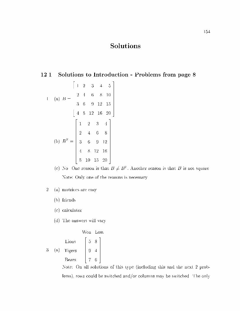
154
Solutions
12.1 Solutions to Introduction - Problems from page 8
1. (a) B =
26666666664
1 2 3 4 5
2 4 6 8 10
3 6 9 12 15
4 8 12 16 20
37777777775
(b) BT =
266666666666664
1 2 3 4
2 4 6 8
3 6 9 12
4 8 12 16
5 10 15 20
377777777777775
(c) No. One reason is that B 6= BT: Another reason is that B is not square.
Note: Only one of the reasons is necessary.
2. (a) matrices are easy
(b) friends
(c) calculator
(d) The answers will vary.
3. (a)
Lions
Tigers
Bears
Won Lost2666664
5 8
9 4
7 6
3777775
Note: On all solutions of this type (including this and the next 2 prob-
lems), rows could be switched and/or columns may be switched. The only

155
requirement is that each of these numbers lines up with both of its labels.
Therefore,
Lions
Bears
Tigers
Lost Won2666664
8 5
6 7
4 9
3777775
is also an appropriate solution.
(b)Won
Lost
L T B264 5 9 7
8 4 6
375
Note: Make sure that this matrix corresponds to the solution that the
student gave on part (a) if the columns or rows were not as we ordered
them in part (a).
4. (a)
Won
Lost
Tied
S L F T2666664
6 8 9 5
8 7 4 9
1 0 2 1
3777775
(b)
Snakes
Lizards
Frogs
Toads
W L T26666666664
6 8 1
8 7 0
9 4 2
5 9 1
37777777775
Please refer to the notes on the previous problem.
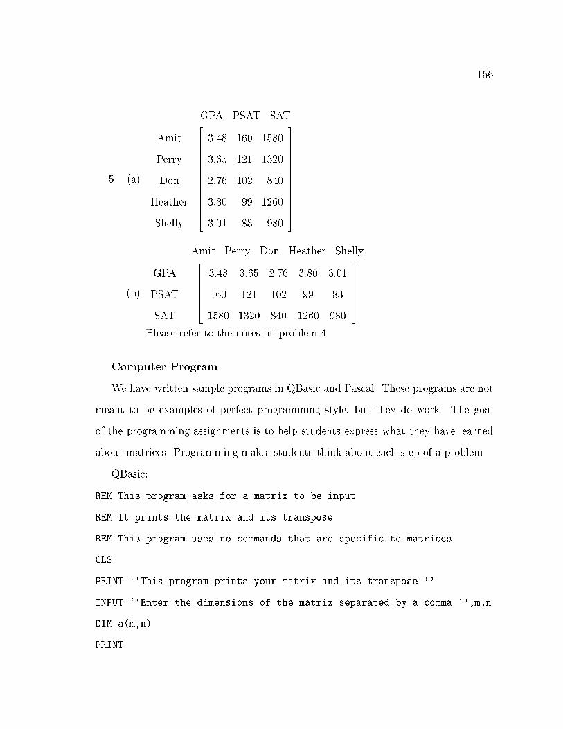
156
5. (a)
Amit
Perry
Don
Heather
Shelly
GPA PSAT SAT266666666666664
3:48 160 1580
3:65 121 1320
2:76 102 840
3:80 99 1260
3:01 83 980
377777777777775
(b)
GPA
PSAT
SAT
Amit Perry Don Heather Shelly2666664
3:48 3:65 2:76 3:80 3:01
160 121 102 99 83
1580 1320 840 1260 980
3777775
Please refer to the notes on problem 4.
Computer Program
We have written sample programs in QBasic and Pascal. These programs are not
meant to be examples of perfect programming style, but they do work. The goal
of the programming assignments is to help students express what they have learned
about matrices. Programming makes students think about each step of a problem.
QBasic:
REM This program asks for a matrix to be input.
REM It prints the matrix and its transpose.
REM This program uses no commands that are specific to matrices.
CLS
PRINT ``This program prints your matrix and its transpose.''
INPUT ``Enter the dimensions of the matrix separated by a comma.'',m,n
DIM a(m,n)

157
PRINT ``Please press enter after each element of the matrix. ''
PRINT ``Enter all the elements of one row before the next row. ''
REM This loop reads the matrix
FOR i=1 to m
FOR j=1 to n
INPUT a(i,j)
NEXT j
NEXT i
REM This loop prints the matrix
PRINT ``This is the matrix that you entered: ''
FOR i=1 to m
FOR j=1 to n
PRINT a(i,j),
NEXT j
NEXT i
REM This loop prints the transpose of the matrix
PRINT ``This is the transpose of your matrix: ''
FOR j=1 to n
FOR i=1 to m
PRINT a(i,j),

158
NEXT i
NEXT j
END
Pascal:
Program intro(input, output);
{This program asks for a matrix to be input.
It prints the matrix and its transpose.
This program uses no commands that are specific to matrices.}
uses crt; {Necessary for some Pascal compilers}
type
matrix=array[1..10,1..10] of real;
var
m,n: integer; {dimensions of the matrices}
a: matrix; {matrix}
procedure readmatrix(var a:matrix; m,n:integer);
var
i,j: integer; {counters}
begin {read}

159
for i:=1 to m do
begin {do}
for j:=1 to n do
read(a[i,j]);
readln;
end; {do}
end; {read}
procedure writematrix(a:matrix; m,n:integer);
var
i,j: integer; {counters}
begin {write}
for i:=1 to m do
begin {each line}
writeln;
for j:=1 to n do
write(a[i,j]:6:2);
end; {each line}
writeln;
end; {write}
procedure writetranspose(a:matrix; m,n:integer);
var
i,j: integer; {counters}

160
begin {write}
for j:=1 to n do
begin {each line}
writeln;
for i:=1 to m do
write(a[i,j]:6:2);
end; {each line}
writeln;
end; {write}
begin{main program}
clrscr;
writeln('Enter the dimensions of the matrix ');
writeln('separated by a space. Then hit return.');
read(m,n);
writeln('Enter your matrix.');
writeln('Enter each element followed by a return.');
writeln('Enter the first row before you go to the next row.');
readmatrix(a,m,n);
writeln('The matrix that you entered is :');
writematrix(a,m,n);
writeln('The transpose of your matrix is :');
writetranspose(a,m,n);
writeln('Press return to leave the program');
readln;
end. {main program}

161
12.2 Solutions to Addition - Problems from page 15
1. (a) A+ C =
2666664
8 13 8 8
16 7 6 7
4 13 13 4
3777775
(b) D + E =
26666666664
7 11 5
18 13 2
6 6 7
7 13 6
37777777775
(c) F �D =
26666666664
2 �4 �2
�9 �1 2
7 4 1
�3 �5 7
37777777775
(d) F +B =not possible since the dimensions do not match.
(e) B � (A+ C) =
2666664
0 �6 �4 �8
�7 �1 �4 �2
�3 �9 �6 �2
3777775
(f) D � (E + F ) =
26666666664
�2 �1 0
0 �7 �3
�13 �8 �4
3 �2 �12
37777777775
(g) B + C � B =
2666664
1 9 0 2
7 4 6 5
3 8 7 1
3777775
(h) A�D =not possible since the dimensions do not match.
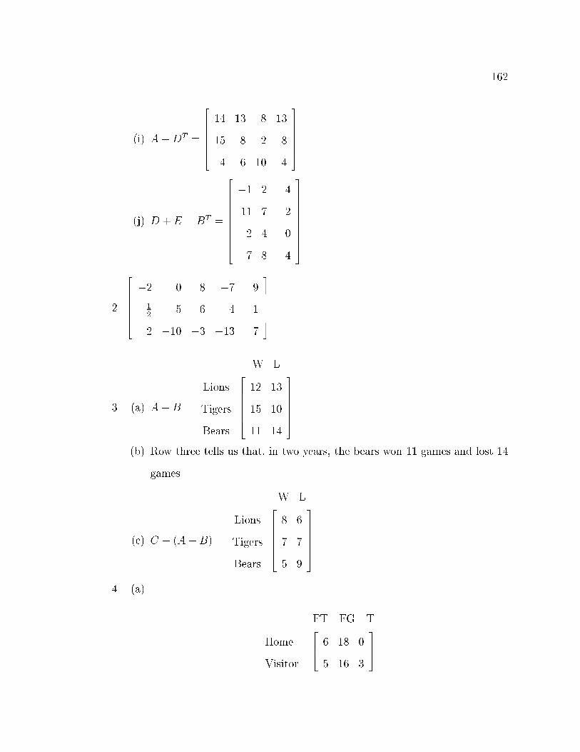
162
(i) A+DT =
2666664
14 13 8 13
15 8 2 8
4 6 10 4
3777775
(j) D + E � BT =
26666666664
�1 2 4
11 7 �2
2 4 0
7 8 4
37777777775
2.
2666664
�2 0 8 �7 9
�12
�5 6 �4 �1
2 �10 �3 �13 7
3777775
3. (a) A+B =
Lions
Tigers
Bears
W L2666664
12 13
15 10
11 14
3777775
(b) Row three tells us that, in two years, the bears won 11 games and lost 14
games.
(c) C � (A+B) =
Lions
Tigers
Bears
W L2666664
8 6
7 7
5 9
3777775
4. (a)
Home
Visitor
FT FG T264 6 18 0
5 16 3
375

163
(b) Home won 85 to 84.
5. Yes. This can be proven using the facts learned in the Questions and Answers
in Chapters 1 and 2. The matrix (A + AT )
T= A
T +(AT )T= A
T +A = A+AT .
6. Yes. The matrices A and B must both be square because they are symmetric.
Therefore, if they have the same dimensions, then A� B must also be square.
A generic element of A � B is aij � bij. Since A and B are symmetric, this
element is the same as aji � bji which is also a generic element for (A�B)T
because (A�B)T= A
T�B
T . Therefore, A� B is symmetric.
Computer Program
QBasic:
REM This program adds and subtracts matrices
REM It uses no commands that are specific to matrices
CLS
PRINT ``This program will add or subtract matrices. ''
INPUT ``Enter the dimensions of the matrices separated by a comma.'',m,n
DIM a(m,n)
DIM b(m,n)
REM This loop reads the first matrix
PRINT ``Please press enter after each element of the matrix. ''
PRINT ``Enter all the elements of one row before the next row. ''
FOR i=1 to m
FOR j=1 to n
INPUT a(i,j)
NEXT j

164
NEXT i
100 REM This allows the user to choose what to do next
INPUT ``Do you wish to 1) add 2) subtract or 3) end '',s
IF s=3 then goto 500
200 PRINT ``Enter the next matrix. ''
FOR i=1 to m
FOR j=1 to n
INPUT b(i,j)
NEXT j
NEXT i
If s=1 then GOSUB 1000 ELSE IF s=2 THEN GOSUB 2000 ELSE IF s=3
THEN GOTO 500 ELSE GOTO 100
REM The previous line should be part of the line above it
PRINT ``The resulting matrix is: ''
FOR i=1 to m
FOR j=1 to n
PRINT a(i,j),
NEXT j
NEXT i
GOTO 100
500 PRINT ``Your final solution is: ''
FOR i=1 to m

165
FOR j=1 to n
PRINT a(i,j),
NEXT j
NEXT i
END
1000 REM This adds matrices
FOR i=1 to m
FOR i=1 to n
a(i,j)=a(i,j)+b(i,j)
NEXT j
NEXT i
RETURN
2000 REM This subtracts matrices
FOR i=1 to m
FOR i=1 to n
a(i,j)=a(i,j)-b(i,j)
NEXT j
NEXT i
RETURN
Pascal:
Program add(input, output);

166
{This program adds and subtracts matrices.}
uses crt; {Necessary for some Pascal compilers}
type
matrix=array[1..10,1..10] of real;
var
choice : integer; {for choosing operation}
m,n: integer; {dimensions of the matrices}
a,b: matrix; {matrix}
procedure readmatrix(var a:matrix; m,n:integer);
var
i,j: integer; {counters}
begin {read}
for i:=1 to m do
begin {do}
for j:=1 to n do
read(a[i,j]);
readln;
end {do}
end; {read}
procedure writematrix(a:matrix; m,n:integer);

167
var
i,j: integer; {counters}
begin {write}
for i:=1 to m do
begin {each line}
writeln;
for j:=1 to n do
write(a[i,j]:6:2);
end; {each line}
writeln;
end; {write}
procedure addmatrix(var a:matrix; b: matrix);
var
i,j: integer; {counters}
begin {addmatrix}
for i:=1 to m do
for j:=1 to n do
a[i,j]:=a[i,j]+b[i,j];
end;{addmatrix}
procedure submatrix(var a:matrix; b: matrix);
var
i,j: integer; {counters}

168
begin {submatrix}
for i:=1 to m do
for j:=1 to n do
a[i,j]:=a[i,j]-b[i,j];
end;{submatrix}
procedure menu{(var choice:char)};
begin {menu}
writeln;
writeln('Do you wish to :');
writeln(' 1. Add');
writeln(' 2. Subtract');
writeln(' 3. End the program');
readln(choice);
end;{menu}
procedure operation(var a : matrix);
begin {operation}
writeln('Enter your second matrix.');
writeln('Enter the elements of each row separated');
writeln('by a space. Hit return at the end of each row.');
readmatrix(b,m,n);
if choice = 1 then
addmatrix(a,b)
else if choice = 2 then

169
submatrix(a,b)
else if choice = 3 then
choice := 3
else if ((choice <> 1) and (choice <> 2) and (choice <> 3)) then
begin {else if}
writeln('That was not a choice.');
choice := 4;
end;{else if}
end;{operation}
begin{main program}
clrscr;
choice := 0;
writeln('Enter the dimensions of the matrix ');
writeln('separated by a space. Then hit return.');
read(m,n);
writeln('Enter your matrix.');
writeln('Enter each element followed by a return.');
writeln('Enter the first row before you go to the next row.');
readmatrix(a,m,n);
menu;
while choice <> 3 do
begin {while}
operation(a);
writeln('The resulting matrix is :');
writematrix(a,m,n);

170
menu
end; {while}
writeln('The final resulting matrix is :');
writematrix(a,m,n);
writeln('Press return to leave the program');
readln;
end. {main program}
12.3 Solutions to Multiplication - Problems from page 30
1. (a) Symmetric
(b) Multiply the matrix by the scalar 1.6
(c)
26666666664
0 2464 2576 2192
2464 0 4464 4240
2576 4464 0 384
2192 4240 384 0
37777777775
2. (a) 4C =
�20 12 24
�
(b) AD =
2666664
94
66
52
3777775
(c) DA - The dimensions are wrong (3 by 1 multiplied by 3 by 3). The inside
dimensions do not agree.
(d) BC - The dimensions are wrong (3 by 3 multiplied by 1 by 3). The inside
dimensions do not agree.
(e) 3CB =
�342 213 180
�
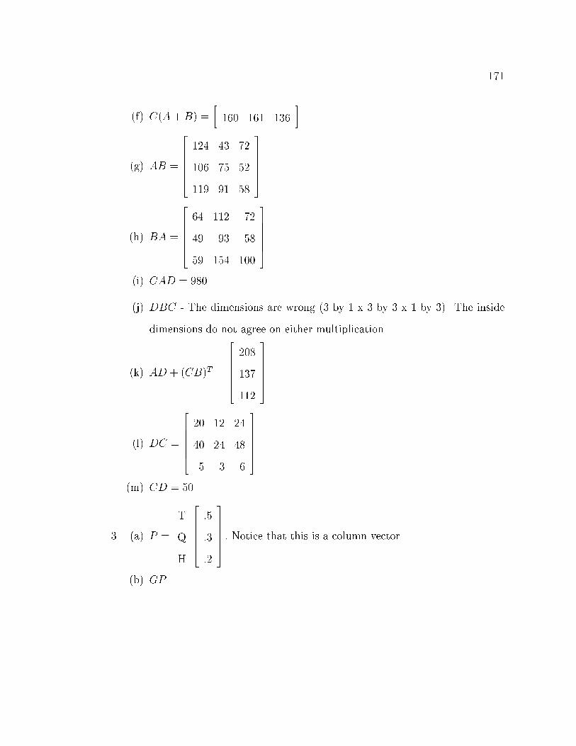
171
(f) C(A+B) =
�160 161 136
�
(g) AB =
2666664
124 43 72
106 75 52
119 91 58
3777775
(h) BA =
2666664
64 112 72
49 93 58
59 154 100
3777775
(i) CAD = 980
(j) DBC - The dimensions are wrong (3 by 1 x 3 by 3 x 1 by 3). The inside
dimensions do not agree on either multiplication.
(k) AD + (CB)T =
2666664
208
137
112
3777775
(l) DC =
2666664
20 12 24
40 24 48
5 3 6
3777775
(m) CD = 50
3. (a) P =
T
Q
H
2666664
:5
:3
:2
3777775: Notice that this is a column vector.
(b) GP

172
(c) GP =
266666666666664
78
84
74
67
84
377777777777775
4. Yes. The matrix A =
264 a11 a12
a21 a22
375 ; the vector x =
264 x1
x2
375 ; and the scalar
c = c:
Because the order of multiplication does not matter for real numbers,
c (Ax)?= A (cx)
c
0B@264 a11 a12
a21 a22
375264 x1
x2
3751CA ?
=
264 a11 a12
a21 a22
3750B@c
264 x1
x2
3751CA
c
0B@264 a11x1 + a12x2
a21x1 + a22x2
3751CA ?
=
264 a11 a12
a21 a22
3750B@264 cx1
cx2
3751CA
264 ca11x1 + ca12x2
ca21x1 + ca22x2
375 ?
=
264 a11cx1 + a12cx2
a21cx1 + a22cx2
375
264 ca11x1 + ca12x2
ca21x1 + ca22x2
375 ?
=
264 ca11x1 + ca12x2
ca21x1 + ca22x2
375
Make sure that you tell the students that c(Ax) = A(cx) for all matrices
that have the correct dimensions for Ax to be multiplied.
5.
2666664
a
b
c
3777775
0BBBBB@�d e f
�2666664
g
h
k
3777775
1CCCCCA�l p q
� This grouping requires only 15 simple
multiplications to �nd T:
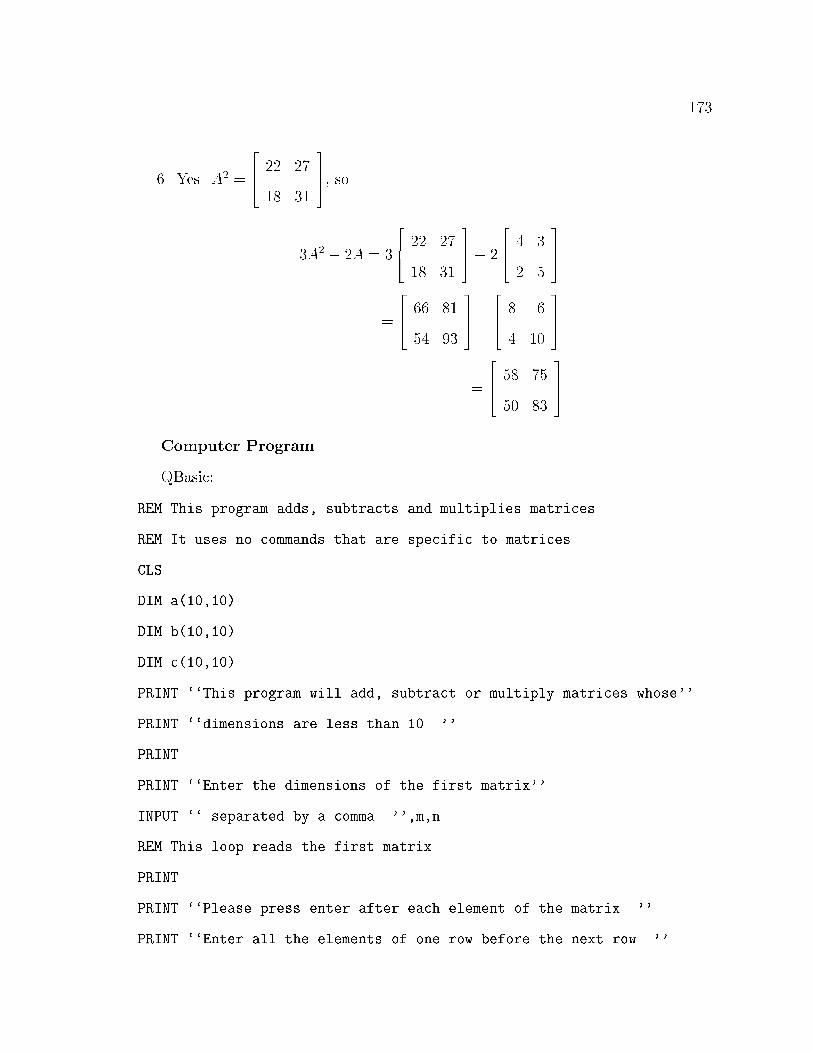
173
6. Yes. A2 =
264 22 27
18 31
375, so
3A2� 2A = 3
264 22 27
18 31
375� 2
264 4 3
2 5
375
=
264 66 81
54 93
375�
264 8 6
4 10
375
=
264 58 75
50 83
375
Computer Program
QBasic:
REM This program adds, subtracts and multiplies matrices
REM It uses no commands that are specific to matrices
CLS
DIM a(10,10)
DIM b(10,10)
DIM c(10,10)
PRINT ``This program will add, subtract or multiply matrices whose''
PRINT ``dimensions are less than 10. ''
PRINT ``Enter the dimensions of the first matrix''
INPUT `` separated by a comma. '',m,n
REM This loop reads the first matrix
PRINT ``Please press enter after each element of the matrix. ''
PRINT ``Enter all the elements of one row before the next row. ''

174
FOR i=1 to m
FOR j=1 to n
INPUT a(i,j)
NEXT j
NEXT i
100 REM This allows the user to choose what to do next.
INPUT ``Do you wish to 1)add 2) subtract 3) multiply or 4) end '',s
IF s=4 THEN GOTO 500
200 PRINT
INPUT ``Enter the dimensions of the next matrix. '',m2,n2
REM The next statements check to make sure the dimensions are correct
REM for the operation
IF (((s=1 or s=2) AND (m<<>m2 OR n<>n2) OR (s=3 AND n<>n2)) THEN
PRINT ``The matrix dimensions are not correct''
GOTO 200
END IF
PRINT ``Enter the next matrix. ''
FOR i=1 to m2
FOR j=1 to n2
INPUT b(i,j)
NEXT j
NEXT i
IF s=1 THEN GOSUB 1000 ELSE IF S=2 THEN GOSUB 2000 ELSE IF S=3

175
THEN GOSUB 3000 ELSE IF S=4 THEN GOTO ELSE GOTO 100
REM The previous line should be part of the one above it
PRINT ``The resulting matrix is: ''
FOR i=1 to m
FOR j=1 to n
PRINT a(i,j),
NEXT j
NEXT i
GOTO 100
500 PRINT
PRINT ``Your final solution is: ''
FOR i=1 to m
FOR j=1 to n
PRINT a(i,j),
NEXT j
NEXT i
END
1000 REM This adds matrices
FOR i=1 to m
FOR j=1 to n
a(i,j)=a(i,j) + b(i,j)
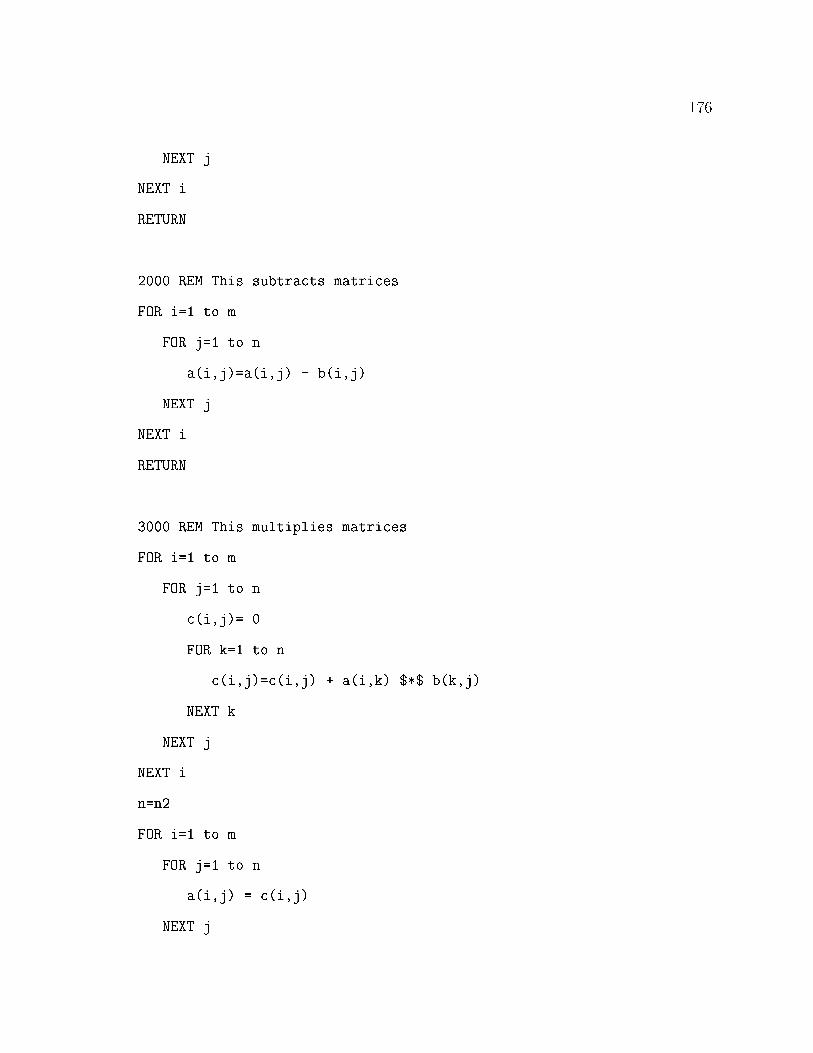
176
NEXT j
NEXT i
RETURN
2000 REM This subtracts matrices
FOR i=1 to m
FOR j=1 to n
a(i,j)=a(i,j) - b(i,j)
NEXT j
NEXT i
RETURN
3000 REM This multiplies matrices
FOR i=1 to m
FOR j=1 to n
c(i,j)= 0
FOR k=1 to n
c(i,j)=c(i,j) + a(i,k) $*$ b(k,j)
NEXT k
NEXT j
NEXT i
n=n2
FOR i=1 to m
FOR j=1 to n
a(i,j) = c(i,j)
NEXT j

177
NEXT i
RETURN
Pascal:
Program mult(input, output);
{This program adds, subtracts, and multiplies matrices.}
uses crt; {Necessary for some Pascal compilers}
type
matrix=array[1..10,1..10] of real;
var
choice : integer; {for choosing operation}
m,n,m2,n2 : integer; {dimensions of the matrices}
a,b,c : matrix; {matrix}
procedure readmatrix(var a:matrix; m,n:integer);
var
i,j: integer; {counters}
begin {read}
for i:=1 to m do
begin {do}
for j:=1 to n do

178
read(a[i,j]);
readln;
end {do}
end; {read}
procedure writematrix(a:matrix; m,n:integer);
var
i,j: integer; {counters}
begin {write}
for i:=1 to m do
begin {each line}
writeln;
for j:=1 to n do
write(a[i,j]:6:2);
end; {each line}
writeln;
end; {write}
procedure addmatrix(var a:matrix; b: matrix);
var
i,j: integer; {counters}
begin {addmatrix}
for i:=1 to m do
for j:=1 to n do

179
a[i,j]:=a[i,j]+b[i,j];
end;{addmatrix}
procedure submatrix(var a:matrix; b: matrix);
var
i,j: integer; {counters}
begin {submatrix}
for i:=1 to m do
for j:=1 to n do
a[i,j]:=a[i,j]-b[i,j];
end;{submatrix}
procedure multmatrix(var a:matrix; b:matrix; m:integer;
var n:integer; m2,n2:integer);
{The above row should be attached to the first row}
var
i,j,k: integer; {counters}
c: matrix; {temporary matrix}
begin {multmatrix}
for i:=1 to m do
for j:=1 to n2 do
begin {inner product}
c[i,j]:=0;
for k:=1 to n do
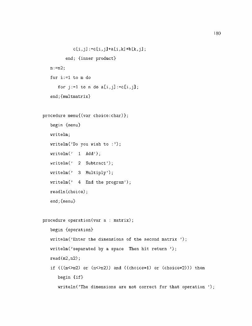
180
c[i,j]:=c[i,j]+a[i,k]*b[k,j];
end; {inner product}
n:=n2;
for i:=1 to m do
for j:=1 to n do a[i,j]:=c[i,j];
end;{multmatrix}
procedure menu{(var choice:char)};
begin {menu}
writeln;
writeln('Do you wish to :');
writeln(' 1. Add');
writeln(' 2. Subtract');
writeln(' 3. Multiply');
writeln(' 4. End the program');
readln(choice);
end;{menu}
procedure operation(var a : matrix);
begin {operation}
writeln('Enter the dimensions of the second matrix ');
writeln('separated by a space. Then hit return.');
read(m2,n2);
if (((m<>m2) or (n<>n2)) and ((choice=1) or (choice=2))) then
begin {if}
writeln('The dimensions are not correct for that operation.');

181
choice := 5;
end {if m}
else if ((choice = 3) and (m2 <> n)) then
begin {else if choice}
writeln('The dimensions are not correct for multiplication.');
choice := 5;
end{elseif choice}
else if ((choice<>1) and (choice<>2) and (choice<>3)
and (choice<>4)) then {this line should be attached
to the previous line}
begin {else if}
writeln('That was not a choice');
choice := 5;
end;{else if}
if (choice<>5) then
begin {if}
writeln('Enter your matrix.);
writeln('Enter the elements of each row separated');
writeln('by a space. Hit return at the end of each row.');
readmatrix(b,m2,n2);
end; {if}
if choice = 1 then
addmatrix(a,b)
else if choice = 2 then
submatrix(a,b)
else if choice = 3 then

182
multmatrix(a,b,m,n,m2,n2);
end;{operation}
begin{main program}
clrscr;
choice := 0;
writeln('Enter the dimensions of the first matrix ');
writeln('separated by a space. Then hit return.');
read(m,n);
writeln('Enter your matrix.);
writeln('Enter each element followed by a return.');
writeln('Enter the first row before you go to the next row.');
readmatrix(a,m,n);
menu;
while choice <> 4 do
begin {while}
operation(a);
writeln('The resulting matrix is :');
writematrix(a,m,n);
menu
end; {while}
writeln('The final resulting matrix is :');
writematrix(a,m,n);
writeln('Press return to leave the program');
readln;
end. {main program}
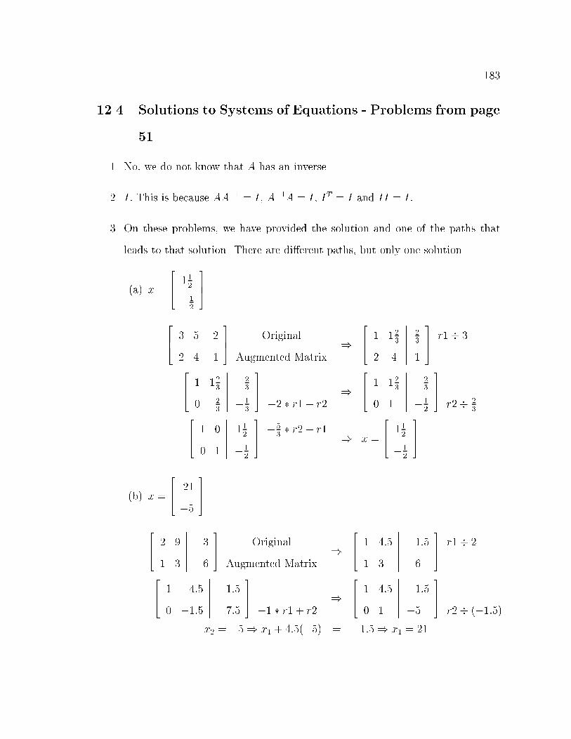
183
12.4 Solutions to Systems of Equations - Problems from page
51
1. No, we do not know that A has an inverse.
2. I: This is because AA�1 = I, A�1A = I; I
T = I and II = I:
3. On these problems, we have provided the solution and one of the paths that
leads to that solution. There are di�erent paths, but only one solution.
(a) x =
264 11
2
�12
375
264 3 5
2 4
�������2
1
375 Original
Augmented Matrix)
264 1 12
3
2 4
�������23
1
375 r1� 3
264 1 12
3
0 23
�������23
�13
375�2 � r1 + r2
)
264 1 12
3
0 1
�������23
�12
375r2� 2
3264 1 0
0 1
�������112
�12
375 �
53� r2 + r1
) x =
264 11
2
�12
375
(b) x =
264 21
�5
375
264 2 9
1 3
��������3
6
375 Original
Augmented Matrix)
264 1 4:5
1 3
��������1:5
6
375 r1� 2
264 1 4:5
0 �1:5
��������1:5
7:5
375�1 � r1 + r2
)
264 1 4:5
0 1
��������1:5
�5
375r2� (�1:5)
x2 = �5) x1 + 4:5(�5) = �1:5) x1 = 21

184
(c) x =
2666664
3
0
�1
3777775
2666664
1 2 1
2 6 3
3 8 5
�����������
2
3
4
3777775
Original
Augmented
Matrix
)
2666664
1 2 1
0 2 1
0 2 2
�����������
2
�1
�2
3777775 �2r1 + r2
�3r1 + r32666664
1 2 1
0 1 :5
0 2 2
�����������
2
�:5
�2
3777775 r2� 2 )
2666664
1 2 1
0 1 :5
0 0 1
�����������
2
�:5
�1
3777775�2 � r2 + r3
2666664
1 2 0
0 1 0
0 0 1
�����������
3
0
�1
3777775
�1 � r3 + r1
�:5 � r3 + r2 )
2666664
1 0 0
0 1 0
0 0 1
�����������
3
0
�1
3777775
�2 � r2 + r1
(d) x =
2666664
3
�3
6
3777775
2666664
2 3 1
1 3 3
3 3 1
�����������
3
12
6
3777775
Original
Augmented
Matrix2666664
1 1:5 0:5
1 3 3
3 3 1
�����������
1:5
12
6
3777775
r1� 2
2666664
1 1:5 0:5
0 1:5 2:5
0 �1:5 �0:5
�����������
1:5
10:5
1:5
3777775 �1 � r1 + r2
�3 � r1 + r3

185
2666664
1 1:5 0:5
0 1 123
0 �1:5 �0:5
�����������
1:5
7
1:5
3777775 r2� 1:5
2666664
1 1:5 0:5
0 1 123
0 0 2
�����������
1:5
7
12
3777775
1:5 � r2 + r32666664
1 1:5 0:5
0 1 123
0 0 1
�����������
1:5
7
6
3777775r3� 2
x3 = 6
x2 + 12
3(6) = 7) �3
x1 + 1:5(�3) + 0:5(6) = 1:5) 3
4. (a)
264
45
�35
�1 1
375 Use the formula that we found for 2 by 2 matrices.
(b)
264 �13
535
125
�25
375 Use the formula that we found for 2 by 2 matrices.
(c)
2666664
�1 �1 1
1 0 0
0 3 �2
3777775
2666664
0 1 0
2 2 1
3 3 1
�����������
1 0 0
0 1 0
0 0 1
3777775
Original
Augmented
Matrix
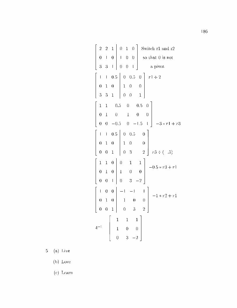
186
2666664
2 2 1
0 1 0
3 3 1
�����������
0 1 0
1 0 0
0 0 1
3777775
Switch r1 and r2
so that 0 is not
a pivot2666664
1 1 0:5
0 1 0
3 3 1
�����������
0 0:5 0
1 0 0
0 0 1
3777775
r1� 2
2666664
1 1 0:5
0 1 0
0 0 �0:5
�����������
0 0:5 0
1 0 0
0 �1:5 1
3777775�3 � r1 + r3
2666664
1 1 0:5
0 1 0
0 0 1
�����������
0 0:5 0
1 0 0
0 3 �2
3777775r3� (�:5)
2666664
1 1 0
0 1 0
0 0 1
�����������
0 �1 1
1 0 0
0 3 �2
3777775�0:5 � r3 + r1
2666664
1 0 0
0 1 0
0 0 1
�����������
�1 �1 1
1 0 0
0 3 �2
3777775�1 � r2 + r1
A�1 =
2666664
�1 �1 1
1 0 0
0 3 �2
3777775
5. (a) Live
(b) Love
(c) Learn
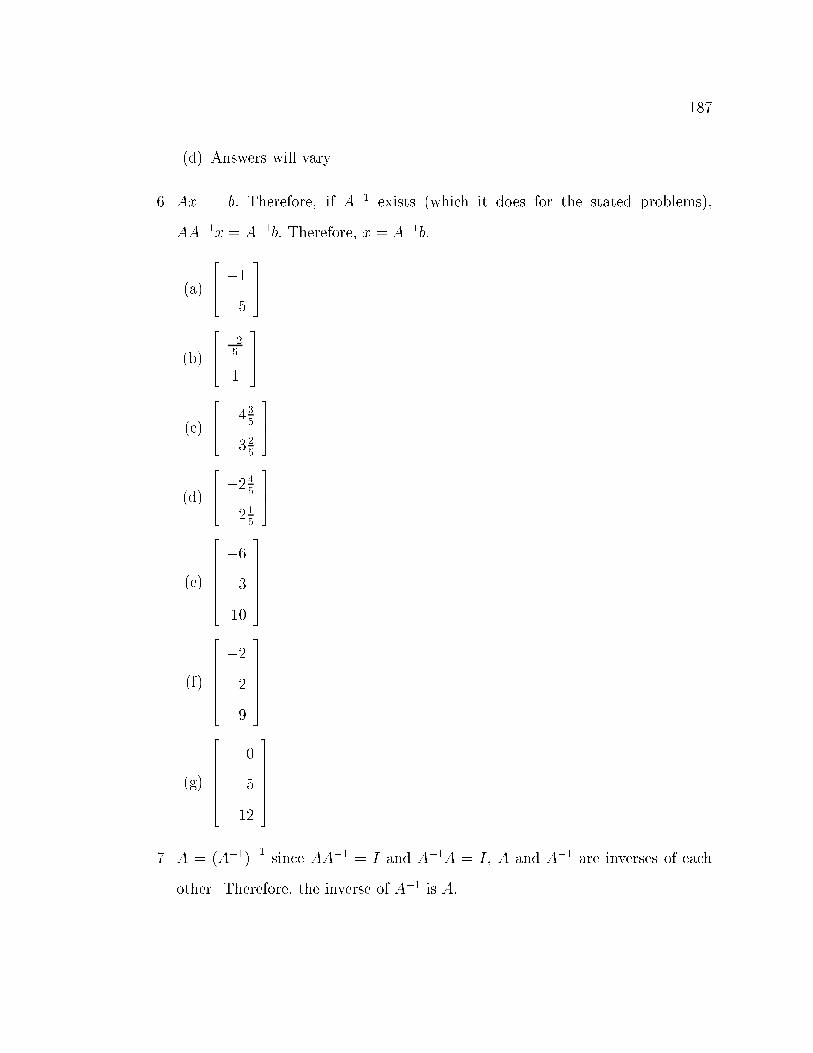
187
(d) Answers will vary
6. Ax = b: Therefore, if A�1 exists (which it does for the stated problems),
AA�1x = A
�1b: Therefore, x = A
�1b:
(a)
264 �1
5
375
(b)
264
�25
1
375
(c)
264 43
5
�325
375
(d)
264 �24
5
215
375
(e)
2666664
�6
3
10
3777775
(f)
2666664
�2
�2
9
3777775
(g)
2666664
0
5
�12
3777775
7. A = (A�1)�1
since AA�1 = I and A�1A = I, A and A
�1 are inverses of each
other. Therefore, the inverse of A�1 is A:

188
8. (a)
2666664
1a
0 0
0 1b
0
0 0 1c
3777775
(b) If A is a diagonal matrix consisting of the elements aii; then A�1 is a
diagonal matrix consisting of the elements 1aii:
12.5 Solutions to Determinants - Problems from page 64
1. (a) �10 � 6� 4 = �10
(b) 36 30� (�6) = 36
(c) �211 (18 + 0� 168)� (40 + 0 + 21) = �211
(d) 153 (0 + 75 + 14)� (0� 84 + 20) = 153
(e) �2 (0 + 0 + 0)� (27 + 0� 25) = �2
(f) �44 (�1)(�2)
�����������
�4 2 1
5 0 �2
2 �1 0
�����������+(�1)(2)
�����������
3 7 6
�4 2 1
2 �1 0
�����������is one method.
(g) �510 (+1)(�3)
�����������
9 3 1
�2 6 �4
2 �1 4
�����������
(h) 151 (�1)(2)
�����������
3 1 0
�5 6 2
8 �3 1
�����������+ (+1)(�1)
�����������
7 3 1
�2 �5 6
0 8 �3
�����������
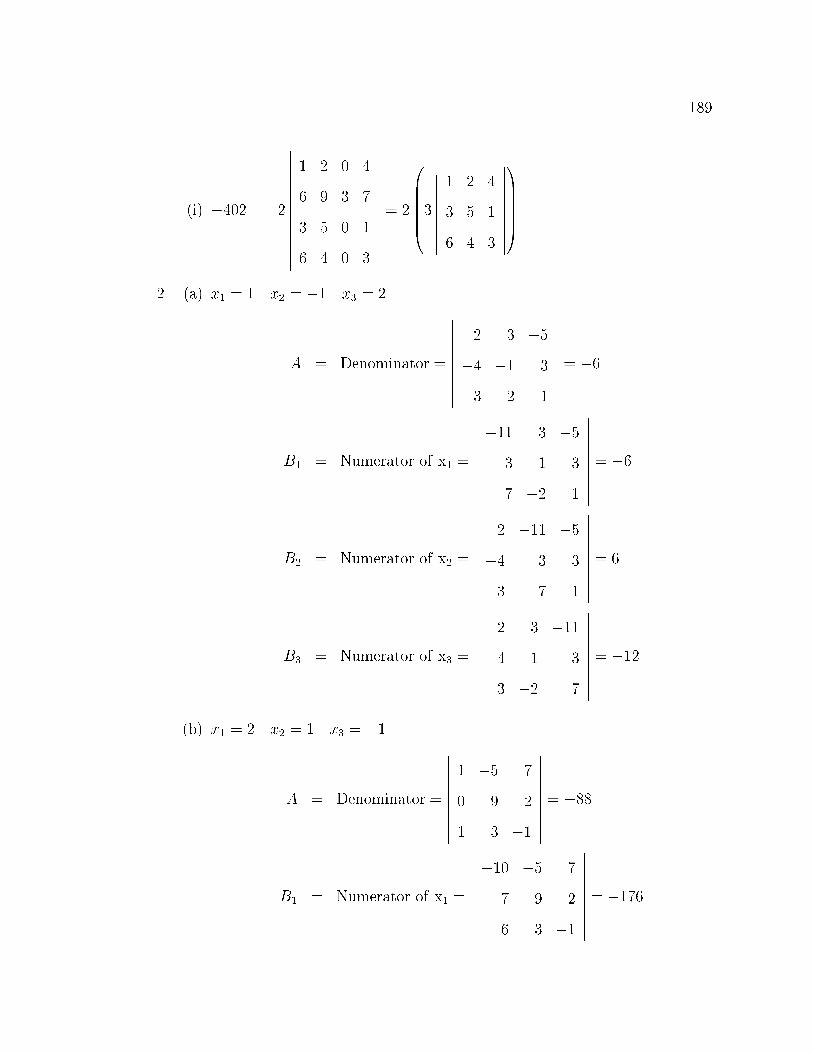
189
(i) �402 2
���������������
1 2 0 4
6 9 3 7
3 5 0 1
6 4 0 3
���������������
= 2
0BBBBB@3
�����������
1 2 4
3 5 1
6 4 3
�����������
1CCCCCA
2. (a) x1 = 1 x2 = �1 x3 = 2
A = Denominator =
�����������
2 3 �5
�4 �1 3
3 �2 1
�����������= �6
B1 = Numerator of x1 =
�����������
�11 3 �5
3 �1 3
7 �2 1
�����������= �6
B2 = Numerator of x2 =
�����������
2 �11 �5
�4 3 3
3 7 1
�����������= 6
B3 = Numerator of x3 =
�����������
2 3 �11
�4 �1 3
3 �2 7
�����������= �12
(b) x1 = 2 x2 = 1 x3 = �1
A = Denominator =
�����������
1 �5 7
0 9 2
1 3 �1
�����������= �88
B1 = Numerator of x1 =
�����������
�10 �5 7
7 9 2
6 3 �1
�����������= �176
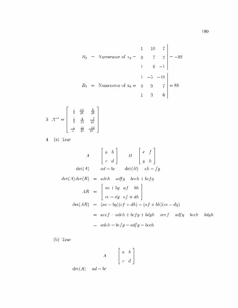
190
B2 = Numerator of x2 =
�����������
1 �10 7
0 7 2
1 6 �1
�����������= �88
B3 = Numerator of x3 =
�����������
1 �5 �10
0 9 7
1 3 6
�����������= 88
3. A�1 =
2666664
15
�125
825
15
425
�725
�15
1125
�1325
3777775
4. (a) True
A =
264 a b
c d
375 B =
264 e f
g h
375
det(A) = ad� bc det(B) = eh� fg
det(A) det(B) = adeh� adfg � bceh + bcfg
AB =
264 ae + bg af + bh
ce + dg cf + dh
375
det(AB) = (ae + bg)(cf + dh)� (af + bh)(ce + dg)
= acef + adeh+ bcfg + bdgh� acef � adfg � bceh� bdgh
= adeh + bcfg � adfg � bceh
(b) True
A =
264 a b
c d
375
det(A) = ad� bc
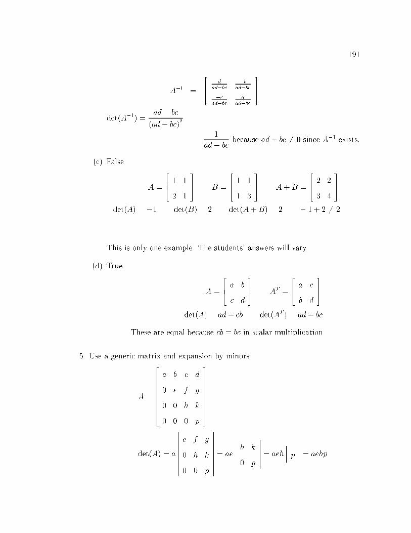
191
A�1 =
264
d
ad�bc
�b
ad�bc
�c
ad�bc
a
ad�bc
375
det(A�1) =ad� bc
(ad� bc)2
=1
ad� bc
because ad� bc 6= 0 since A�1 exists:
(c) False
A =
264 1 1
2 1
375 B =
264 1 1
1 3
375 A +B =
264 2 2
3 4
375
det(A) = �1 det(B) = 2 det(A+B) = 2 � 1 + 2 6= 2
This is only one example. The students' answers will vary.
(d) True
A =
264 a b
c d
375 A
T =
264 a c
b d
375
det(A) = ad� cb det(AT ) = ad� bc
These are equal because cb = bc in scalar multiplication
5. Use a generic matrix and expansion by minors.
A =
26666666664
a b c d
0 e f g
0 0 h k
0 0 0 p
37777777775
det(A) = a
�����������
e f g
0 h k
0 0 p
�����������= ae
�������h k
0 p
�������= aeh
���� p���� = aehp
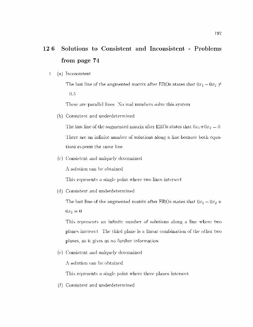
192
12.6 Solutions to Consistent and Inconsistent - Problems
from page 74
1. (a) Inconsistent
The last line of the augmented matrix after EROs states that 0x1 +0x2 6=
�0:5.
These are parallel lines. No real numbers solve this system.
(b) Consistent and underdetermined
The last line of the augmented matrix after EROs states that 0x1+0x2 = 0.
There are an in�nite number of solutions along a line because both equa-
tions express the same line.
(c) Consistent and uniquely determined
A solution can be obtained.
This represents a single point where two lines intersect.
(d) Consistent and underdetermined
The last line of the augmented matrix after EROs states that 0x1 + 0x2 +
0x3 = 0.
This represents an in�nite number of solutions along a line where two
planes intersect. The third plane is a linear combination of the other two
planes, so it gives us no further information.
(e) Consistent and uniquely determined
A solution can be obtained.
This represents a single point where three planes intersect.
(f) Consistent and underdetermined

193
The last two lines of the augmented matrix after EROs states that 0x1 +
0x2 + 0x3 = 0.
This system has an in�nite number of solutions in a plane. All three
equations represent the same plane.
(g) Inconsistent
The last line of the augmented matrix after EROs states that 0x1 + 0x2 +
0x3 6= �0:5.
This represents parallel planes. No real numbers solve this system because
no real numbered solution lies in the intersection of these three planes. This
tells us that at least two of the planes must be parallel to one another. Note
that they do not all three have to be parallel. Even if two planes intersect,
if the third plane is parallel to one of the �rst two planes, there will be no
point that lies in all three planes.
2. Those that are consistent and uniquely determined - c and e.
12.7 Solutions to First Review from page 75
This review is quite long, but it provides a thorough review of the information covered.
You might want to give the students a few days to work on this assignment. If they
can work all these problems, then the test should not be di�cult.
1. 2 by 3
2. B =
2666664
b11 b12 b13 b14
b21 b22 b23 b24
b31 b32 b33 b34
3777775
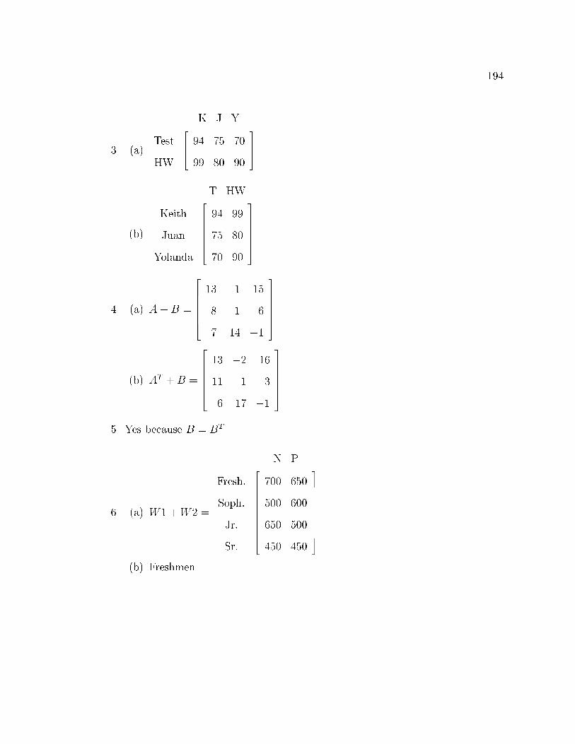
194
3. (a)Test
HW
K J Y264 94 75 70
99 80 90
375
(b)
Keith
Juan
Yolanda
T HW2666664
94 99
75 80
70 90
3777775
4. (a) A+B =
2666664
13 1 15
8 �1 6
7 14 �1
3777775
(b) AT +B =
2666664
13 �2 16
11 �1 3
6 17 �1
3777775
5. Yes because B = BT
6. (a) W1 +W2 =
Fresh:
Soph:
Jr:
Sr:
N P26666666664
700 650
500 600
650 500
450 450
37777777775
(b) Freshmen

195
(c) T � (W1 +W2) =
Fresh:
Soph:
Jr:
Sr:
N P26666666664
300 200
200 150
250 200
150 150
37777777775
(d) 2900
(e)
26666666664
1000 850
700 750
900 700
600 600
37777777775
264 0:3
0:2
375 =
26666666664
470
360
410
300
37777777775These solutions are given in dollars be-
cause we represented 30 cents as 0.3.
(f) $1540
7. (a) No because the inside dimensions of 2 by 3 multiplied by 2 by 3 do not
match.
(b) ABT =
264 54 87
�5 15
375, BAT =
264 54 �5
87 15
375 ; BBT =
264 65 0
0 90
375 : Remember
that the students were only asked for 2 of these.
8. AB =
2666664
48 121 101
�49 �20 5
55 90 121
3777775
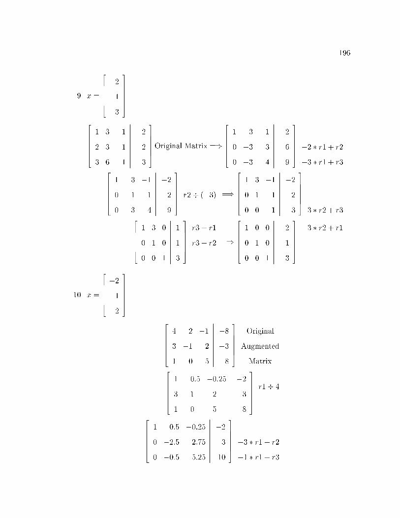
196
9. x =
2666664
�2
1
3
3777775
2666664
1 3 �1
2 3 1
3 6 1
�����������
�2
2
3
3777775Original Matrix =)
2666664
1 3 �1
0 �3 3
0 �3 4
�����������
�2
6
9
3777775 �2 � r1 + r2
�3 � r1 + r32666664
1 3 �1
0 1 �1
0 �3 4
�����������
�2
�2
9
3777775 r2� (�3) =)
2666664
1 3 �1
0 1 �1
0 0 1
�����������
�2
�2
3
3777775
3 � r2 + r32666664
1 3 0
0 1 0
0 0 1
�����������
1
1
3
3777775
r3 + r1
r3 + r2 =)
2666664
1 0 0
0 1 0
0 0 1
�����������
�2
1
3
3777775
�3 � r2 + r1
10. x =
2666664
�2
1
2
3777775
2666664
4 2 �1
3 �1 2
1 0 5
�����������
�8
�3
8
3777775
Original
Augmented
Matrix2666664
1 0:5 �0:25
3 �1 2
1 0 5
�����������
�2
�3
8
3777775r1� 4
2666664
1 0:5 �0:25
0 �2:5 2:75
0 �0:5 5:25
�����������
�2
3
10
3777775 �3 � r1 + r2
�1 � r1 + r3
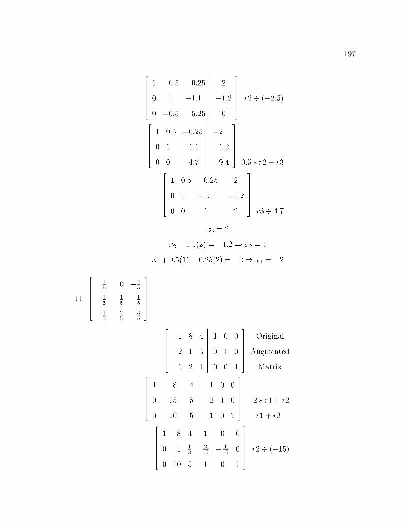
197
2666664
1 0:5 �0:25
0 1 �1:1
0 �0:5 5:25
�����������
�2
�1:2
10
3777775 r2� (�2:5)
2666664
1 0:5 �0:25
0 1 �1:1
0 0 4:7
�����������
�2
�1:2
9:4
3777775
0:5 � r2 + r32666664
1 0:5 �0:25
0 1 �1:1
0 0 1
�����������
�2
�1:2
2
3777775r3� 4:7
x3 = 2
x2 � 1:1(2) = �1:2) x2 = 1
x1 + 0:5(1)� 0:25(2) = �2) x1 = �2
11.
2666664
15
0 �45
15
�15
�15
�15
25
35
3777775
2666664
1 8 4
2 1 3
�1 2 1
�����������
1 0 0
0 1 0
0 0 1
3777775
Original
Augmented
Matrix2666664
1 8 4
0 �15 �5
0 10 5
�����������
1 0 0
�2 1 0
1 0 1
3777775 �2 � r1 + r2
r1 + r32666664
1 8 4
0 1 13
0 10 5
�����������
1 0 0
215
�115
0
1 0 1
3777775 r2� (�15)

198
2666664
1 8 4
0 1 13
0 0 123
�����������
1 0 0
215
�115
0
�13
23
1
3777775�10 � r2 + r3
2666664
1 8 4
0 1 13
0 0 1
�����������
1 0 0
215
�115
0
�15
25
35
3777775r3� 12
32666664
1 8 0
0 1 0
0 0 1
�����������
145
�135
�225
15
�15
�15
�15
25
35
3777775
�4 � r3 + r1
�13� r3 + r2
2666664
1 0 0
0 1 0
0 0 1
�����������
15
0 �45
15
�15
�15
�15
25
35
3777775
�8 � r2 + r1
12. No. If the matrix is inconsistent or underdetermined, an inverse will not exist
because there is not a matrix such that AA�1 = A�1A = I:
13. (a) �2 (�8)� (�6) = �2
(b) 140 (0 + 216� 12)� (0� 8 + 72) = 140
(c) 940 2
�����������
�5 4 4
2 1 6
3 7 2
�����������+
�����������
7 9 �6
�5 4 4
3 7 2
�����������= 940
(d) �120 2
���������������
6 6 0 1
�9 �8 4 7
0 3 0 0
1 10 0 1
���������������
= 2(3)
�����������
6 0 1
�9 4 7
1 0 1
�����������= �120
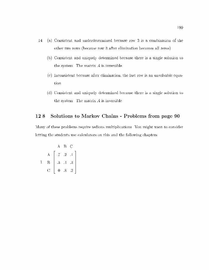
199
14. (a) Consistent and underdetermined because row 3 is a combination of the
other two rows (because row 3 after elimination becomes all zeros).
(b) Consistent and uniquely determined because there is a single solution to
the system. The matrix A is invertible.
(c) Inconsistent because after elimination, the last row is an unsolvable equa-
tion.
(d) Consistent and uniquely determined because there is a single solution to
the system. The matrix A is invertible.
12.8 Solutions to Markov Chains - Problems from page 90
Many of these problems require tedious multiplications. You might want to consider
letting the students use calculators on this and the following chapters.
1.
A
B
C
A B C2666664
:7 :2 :1
:3 :4 :3
0 :8 :2
3777775

200
2. (a)
A C
B
D
.25 1
.5
.2
.15 .5
.1.3.4
.4
.2
(b) Information that ows into C never leaves. Since matter has a way to get
to C from A and B, and because matter can never leave C once it ows
into C, eventually, C should absorb all the matter in the system.
3. (a) Yes. Each element of the transition matrix is a probability. The elements
of each row sum to 1. The matrix has a row and a column for each state.
(b) No. :6 + :1 + :2 = :9 6= 1
(c) No. :25 + :15 + :3 + :4 = 1:1 6= 1
4. (a) No. The probability of leaving B (including the chance of immediately
returning to B) is less than 1.
(b) Yes.
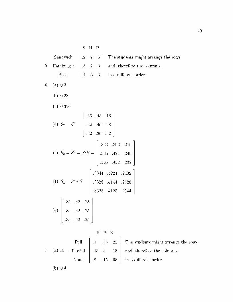
201
5.
Sandwich
Hamburger
Pizza
S H P2666664
:2 :2 :6
:5 :2 :3
:4 :3 :3
3777775
The students might arrange the rows
and, therefore the columns,
in a di�erent order.
6. (a) 0.3
(b) 0.28
(c) 0.336
(d) S2 = S2 =
2666664
:36 :48 :16
:32 :40 :28
:32 :36 :32
3777775
(e) S3 = S3 = S
2S =
2666664
:328 :396 :276
:336 :424 :240
:336 :432 :232
3777775
(f) S4 = S4s3S =
2666664
:3344 :4224 :2432
:3328 :4144 :2528
:3328 :4128 :2544
3777775
(g)
2666664
:33 :42 :25
:33 :42 :25
:33 :42 :25
3777775
7. (a) A =
Full
Partial
None
F P N2666664
:4 :35 :25
:45 :4 :15
:8 :15 :05
3777775
The students might arrange the rows
and, therefore the columns,
in a di�erent order.
(b) 0.4
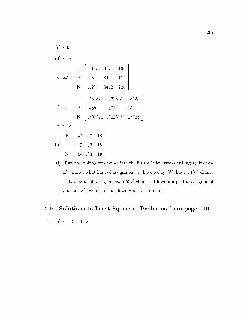
202
(c) 0.05
(d) 0.18
(e) A2 =
F
P
N
2666664
:5175 :3175 :165
:48 :34 :18
:4275 :3475 :225
3777775
(f) A3 =
F
P
N
2666664
:481875 :332875 :18525
:489 :331 :18
:507375 :322375 :17025
3777775
(g) 0.18
(h)
F
P
N
2666664
:49 :33 :18
:49 :33 :18
:49 :33 :18
3777775
(i) If we are looking far enough into the future (a few weeks or longer), it does-
n't matter what kind of assignment we have today. We have a 49% chance
of having a full assignment, a 33% chance of having a partial assignment
and an 18% chance of not having an assignment.
12.9 Solutions to Least Squares - Problems from page 110
1. (a) y = 3� 1:5x
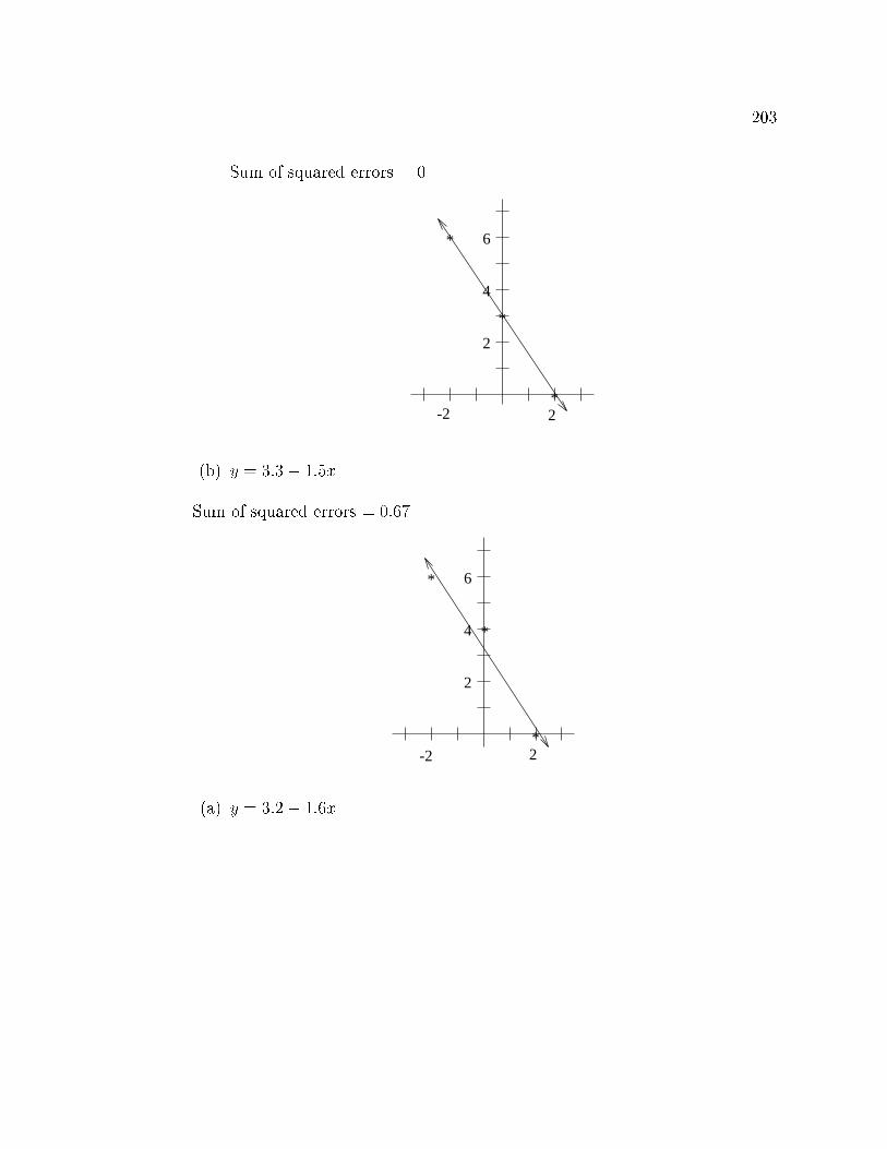
203
Sum of squared errors = 0
*
2
4
6
2
*
*
-2
(b) y = 3:3� 1:5x
Sum of squared errors = 0:67
*
*
2
4
6
2
*
-2
(a) y = 3:2� 1:6x
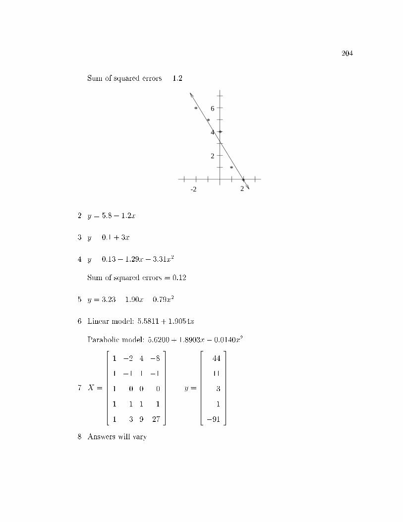
204
Sum of squared errors = 1:2
*
*
2
4
6
2
*
-2
*
*
2. y = 5:8� 1:2x
3. y = 0:1 + 3x
4. y = 0:13� 1:29x+ 3:31x2
Sum of squared errors = 0:12
5. y = 3:23� 1:90x+ 0:79x2
6. Linear model: 5:5811 + 1:9054x
Parabolic model: 5:6200 + 1:8903x� 0:0140x2
7. X =
266666666666664
1 �2 4 �8
1 �1 1 �1
1 0 0 0
1 1 1 1
1 3 9 27
377777777777775
y =
266666666666664
44
11
3
1
�91
377777777777775
8. Answers will vary.

205
12.10 Solutions to Eigenpairs - Problems from page 130
Note: If your students have never seen the video footage of the Tacoma Bridge dis-
aster, it is well worth your time to �nd it and show it to them.
1. x =
2666664
:33
:42
:25
3777775
� = 1
2. x =
2666664
:49
:33
:18
3777775
� = 1
3. x =
264 0
1
375 � = 8
4. x =
264 2:5
1
375 � = 4
5. x =
264 5
1
375 � = 4
x =
264 �1
1
375 � = �2
6. x =
264 0
1
375 � = �2
x =
264 3:5
1
375 � = 5

206
7. x =
264 3:5
1
375 � = 5
x =
264 �1
1
375 � = �4
8. The solutions can be any non-zero, constant multiples of
26666666664
�3
2
�1
1
37777777775: Examples
are:
26666666664
�9
6
�3
3
37777777775;
26666666664
�6
4
�2
2
37777777775; and
26666666664
3
�2
1
�1
37777777775:
12.11 Solutions to Second Review from page 140
1. (a) A =
A
B
C
A B C2666664
:6 :3 :1
:2 :6 :2
:2 :1 :7
3777775
(b) .1
(c) .19
(d) A2 =
A
B
C
A B C2666664
:44 :37 :19
:28 :44 :28
:28 :19 :53
3777775

207
(e) A3 =
A
B
C
A B C2666664
:376 :373 :251
:312 :376 :312
:312 :251 :437
3777775
(f) An =
A
B
C
A B C2666664
:3 :3 :3
:3 :3 :3
:3 :3 :3
3777775; where n is large
(g) This means that after many years, a third of the teachers in the district
will be at each school, A, B, and C, regardless of how many teachers are
in each school now.
2. (a) 2x+ 1:5
(b) 3x� 1:5
3. (a) 1:9x2 + 2:8x� 1:1
(b) 3x2 � 2:2x + 1:1
4. (a) � = 1 x =
2666664
:3
:3
:3
3777775
(b) � = 7 x =
264 3
1
375
(c) � = 1 x =
264 4
1
375 and � = �2 x =
264 1
1
375
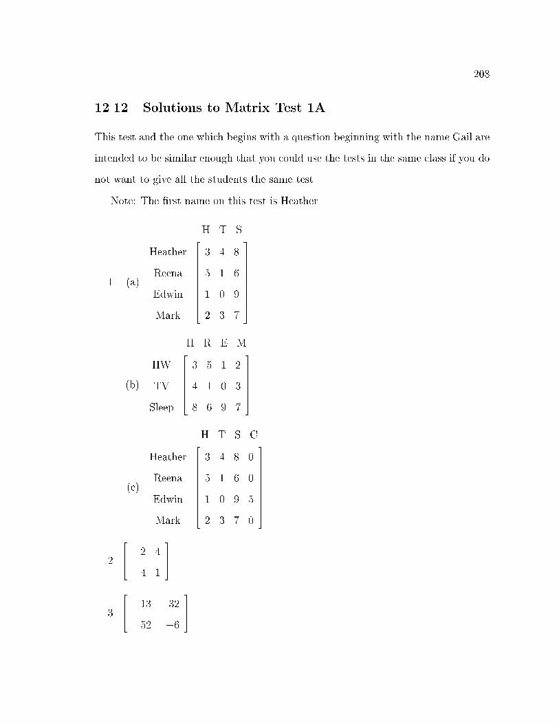
208
12.12 Solutions to Matrix Test 1A
This test and the one which begins with a question beginning with the name Gail are
intended to be similar enough that you could use the tests in the same class if you do
not want to give all the students the same test.
Note: The �rst name on this test is Heather.
1. (a)
Heather
Reena
Edwin
Mark
H T S26666666664
3 4 8
5 1 6
1 0 9
2 3 7
37777777775
(b)
HW
TV
Sleep
H R E M2666664
3 5 1 2
4 1 0 3
8 6 9 7
3777775
(c)
Heather
Reena
Edwin
Mark
H T S C26666666664
3 4 8 0
5 1 6 0
1 0 9 5
2 3 7 0
37777777775
2.
264 �2 4
4 1
375
3.
264 �13 �32
52 �6
375

209
4.
264 1 �3
�12
2
375
5. Augment the matrix with the identity matrix like this:
2666664
3 4 1
1 2 1
�2 2 3
�����������
1 0 0
0 1 0
0 0 1
3777775:
Then perform Gauss-Jordan elimination on the augmented matrix.
The inverse is
2666664
�2 5 �1
2:5 �5:5 1
�3 7 �1
3777775:
Note that the students were only asked for the steps OR the inverse.
6. Answers will vary. Matrix A =
264 a b
b c
375 is a generic 2 by 2 symmetric matrix.
The matrix is symmetric because A = AT:
7. x =
2666664
1
3
2
3777775
Gauss-Jordan elimination uses elementary row operations until the matrix to
the left of the bar is the identity matrix. Gaussian elimination uses elementary
row operations until the matrix to the left of the bar is an upper triangular
matrix. Then it uses back-substitution to �nd the values of x.
8. 116
9. (a) Consistent and uniquely determined because there is a single solution.
(b) Consistent and underdetermined because the last equation does not give
you any extra information.
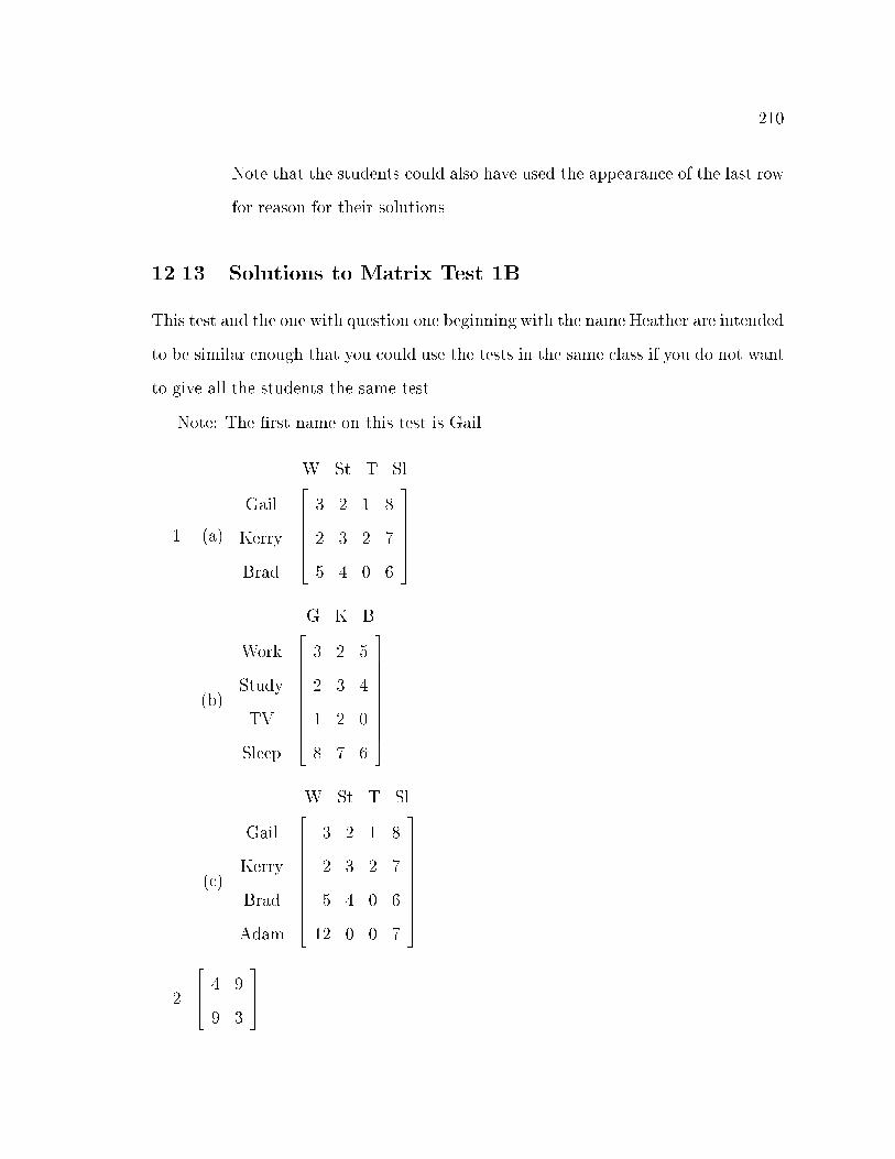
210
Note that the students could also have used the appearance of the last row
for reason for their solutions.
12.13 Solutions to Matrix Test 1B
This test and the one with question one beginning with the name Heather are intended
to be similar enough that you could use the tests in the same class if you do not want
to give all the students the same test.
Note: The �rst name on this test is Gail.
1. (a)
Gail
Kerry
Brad
W St T Sl2666664
3 2 1 8
2 3 2 7
5 4 0 6
3777775
(b)
Work
Study
TV
Sleep
G K B26666666664
3 2 5
2 3 4
1 2 0
8 7 6
37777777775
(c)
Gail
Kerry
Brad
Adam
W St T Sl26666666664
3 2 1 8
2 3 2 7
5 4 0 6
12 0 0 7
37777777775
2.
264 4 9
9 3
375

211
3.
264 14 �33
21 28
375
4.
264 �
13
�113
23
123
375
5. Augment the matrix with the identity matrix like this:
2666664
1 2 1
3 �1 2
1 3 1
�����������
1 0 0
0 1 0
0 0 1
3777775:
Then perform Gauss-Jordan elimination on the augmented matrix.
The inverse is
2666664
�7 1 5
�1 0 1
10 �1 �7
3777775:
Note that the students were only asked for the steps OR the inverse.
6. Answers will vary. Matrix A =
264 a b
b c
375 is a generic 2 by 2 symmetric matrix.
The matrix is symmetric because A = AT:
7. x =
2666664
1
3
2
3777775
Gauss-Jordan elimination uses elementary row operations until the matrix to
the left of the bar is the identity matrix. Gaussian elimination uses elementary
row operations until the matrix to the left of the bar is an upper triangular
matrix. Then it uses back-substitution to �nd the values of x.
8. 22

212
9. (a) Inconsistent because the last equation reduces to an contradictory equa-
tion. Note that the students could also have used the appearance of the
last row for reason for their solutions.
(b) Consistent and uniquely determined because there is a single solution.
12.14 Solutions to Matrix Test 1C
This is the test that begins with a question about Canine Cabins. This test is more
abstract and more di�cult than the other two tests. If your students are advanced,
you might consider using this test. Otherwise, these problems can serve as good
extra credit problems or enrichment problems. This test will also take longer to
grade because many of the questions have answers that may vary, so you will have to
check to make sure the students' answers are correct without the help of an answer
key.
1. (a) Walls =Small
Large
W L P264 25 1 0
70 1 0
375 Roof and F loor =
Small
Large
W L P264 15 1 0
30 1 0
375
(b) Walls+R&F =Small
Large
W L P264 40 2 0
100 2 0
375
(c) Complete =Small
Large
W L P264 40 3:5 1
100 4 1:5
375
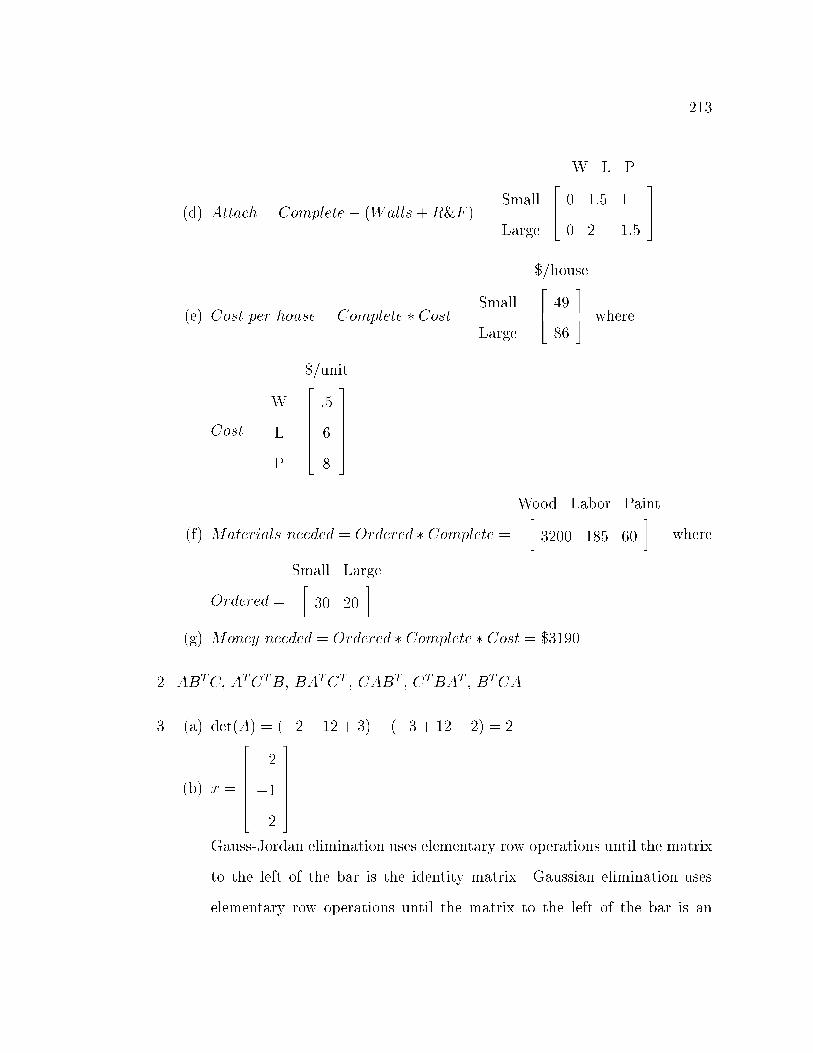
213
(d) Attach = Complete� (Walls+R&F ) =Small
Large
W L P264 0 1:5 1
0 2 1:5
375
(e) Cost per house = Complete � Cost =Small
Large
$=house264 49
86
375 where
Cost =
W
L
P
$=unit2666664
:5
6
8
3777775
(f) Materials needed = Ordered � Complete =
Wood Labor Paint�3200 185 60
�where
Ordered =
Small Large�30 20
�
(g) Money needed = Ordered � Complete � Cost = $3190
2. ABTC; A
TCTB; BA
TCT; CAB
T; C
TBA
T; B
TCA
3. (a) det(A) = (�2 + 12 + 3)� (�3 + 12 + 2) = 2
(b) x =
2666664
2
�1
2
3777775
Gauss-Jordan elimination uses elementary row operations until the matrix
to the left of the bar is the identity matrix. Gaussian elimination uses
elementary row operations until the matrix to the left of the bar is an
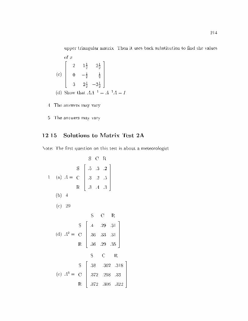
214
upper triangular matrix. Then it uses back substitution to �nd the values
of x.
(c)
2666664
�2 �112
212
0 �12
12
3 212
�312
3777775
(d) Show that AA�1 = A�1A = I.
4. The answers may vary.
5. The answers may vary.
12.15 Solutions to Matrix Test 2A
Note: The �rst question on this test is about a meteorologist.
1. (a) A =
S
C
R
S C R2666664
:5 :3 :2
:3 :2 :5
:3 :4 :3
3777775
(b) .4
(c) .29
(d) A2 =
S
C
R
S C R2666664
:4 :29 :31
:36 :33 :31
:36 :29 :35
3777775
(e) A3 =
S
C
R
S C R2666664
:38 :302 :318
:372 :298 :33
:372 :306 :322
3777775

215
(f) An =
S
C
R
S C R2666664
:375 :302 :323
:375 :302 :323
:375 :302 :323
3777775; where n is large.
(g) The weather will be sunny 37:5% of the time, cloudy 30:2% of the time,
and rainy 32:3% of the time regardless of today's weather.
2. �:5x + 2:1
3. �3:3x2 � 2:0x+ 5:1
4. (a) � = 1 x =
2666664
:375
:302
:323
3777775
(b) � = �5 x =
264 2
1
375
(c) � = 4 x =
264
�32
1
375 and � = �5 x =
264 3
1
375
12.16 Solutions to Matrix Test 2B
Note: The �rst question on this test is about the clothes of a young lady.
1. (a) A =
J
S
D
J S D2666664
:2 :3 :5
:1 :6 :3
:5 :2 :3
3777775
(b) .5
(c) .33

216
(d) A2 =
J
S
D
J S D2666664
:32 :34 :34
:23 :45 :32
:27 :33 :4
3777775
(e) A3 =
J
S
D
J S D2666664
:268 :368 :364
:251 :403 :346
:287 :359 :354
3777775
(f) An =
J
S
D
J S D2666664
:27 :38 :35
:27 :38 :35
:27 :38 :35
3777775; where n is large.
(g) She will wear jeans 27% of the time, slacks 38% of the time, and dresses
35% of the time regardless of what she is wearing today.
2. 5:4x� 3:3
3. x2 � 1:6x+ 2:8
4. (a) � = 1 x =
2666664
:27
:38
:35
3777775
(b) � = �6 x =
264 1:5
1
375
(c) � = 0 x =
264 �3
1
375 and � = 5 x =
264 2
1
375

217
Bibliography
Braun, M. (1983). Di�erential equations and their applications. New York: Springer-
Verlag.
Houston Independent School District. (1992). Houston Independent School District
scope and sequence grades 9-12. Houston, TX: Houston Independent School
District.
National Council of Teachers of Mathematics. (1989). Curriculum and evaluation
standards for school mathematics. Reston, VA: National Council of Teachers
of Mathematics.
Nering, Evar D. (1974). Elementary Linear Algebra. Philadelphia, PA: W.B.
Saunders Company.
Skemp, R. (1987). The psychology of learning mathematics. Hillsdale, NJ: Lawrence
Erlbaum.

218
Index
adding matrices, 11
augmented matrix, 35
back-substitution, 42
by, 4
characteristic equation, 120
cofactor, 56
consistent, 68
counterexample, 7
Cramer's rule, 60
determinant, 54
diagonal matrix, 41
dimensions, 4
dominant eigenvector, 116
dot product, 20
eigenpair, 114
eigenvalue, 114
eigenvector, 114
element, 1, 3
elementary row operations, 34
expansion by minors, 56
Gauss-Jordan elimination, 36
Gaussian elimination, 42
identity matrix, 27, 37
inconsistent, 68, 70
independent, 71
inner product, 20
inverse, 37
least squares, 96, 98
lower triangular, 47
main diagonal, 6
Markov chain, 81, 82
matrices, 3
matrix, 3
matrix product, 23
minor, 56
normal equation, 99
ordered pair, 1
pivot, 40
power method, 116, 117
Rayleigh quotient, 117
scalar, 18
scalar multiplication, 18
scalar product, 19

219
square matrix, 6
state, 80
subtracting matrices, 12
symmetric, 6
transition matrix, 81
transpose, 5
upper triangular, 41
vector, 1
column, 1
row, 1
zero matrix, 13
Top Related