


Languages
Pages
Legal


BME 42-620 Engineering Molecular Cell Biology
Lecture 14:Lecture 14:
Review: Polymer Mechanics
( )Modeling Biochemical Reactions (I)
P j t A i t 02Project Assignment 02
Review: Project Assignment 01
1BME42-620 Lecture 14, October 20, 2011

Outline
• Review: polymer mechanics; Problem set 02• Review: polymer mechanics; Problem set 02
• Modeling biochemical reactionsg
• Project assignment 02
• Review: project assignment 01
2

Outline
• Review: polymer mechanics; Problem set 02• Review: polymer mechanics; Problem set 02
• Modeling biochemical reactionsg
• Project assignment 02
• Review: project assignment 01
3

Basic Mechanical Properties of Cytoskeletal Filamentsp y
• Bending rigidityg g y
• Viscous drag coefficient
• Buckling force
• Persistence length
4

Buckling Forceg• Euler's force: buckling force
on both endson both ends2
2cEIFL
• Example: microtubule buckling fforce
EI=30 10-24N·m2. L = 10 μmFc=6.1pNp
22c
EIFL
5

Persistence Length (I)g ( )
• Persistence length is defined as the characteristic di t d t i d idistance determined in
02
scos s expL
• Persistence length is proportional to the bending rigidity
2 p
pL
and inversely proportional to thermal energy.
EIL pLkT
6

Persistence Length (II)
• Persistence length of cellular filaments
- Actin: 15 m- Microtubule: 6 mm- Keratin intermediate filament: ~ 1 m
- Coiled coil: 100-200 nm- Coiled coil: 100-200 nm- DNA: 50 nm
7

Cytoskeletal Filaments in vivo
• Cytoskeletal filaments
- Highly dynamic in vivo.
- Function in networks.
- Function under tight regulation.
Crosstalk between different filaments- Crosstalk between different filaments.
• Current research focuses on d t di l h i iunderstanding polymer mechanics in
vivo. T. Wittmann et al, J. Cell Biol., 161:845, 2003.
8
Calculation of Diffusion Coefficient
2
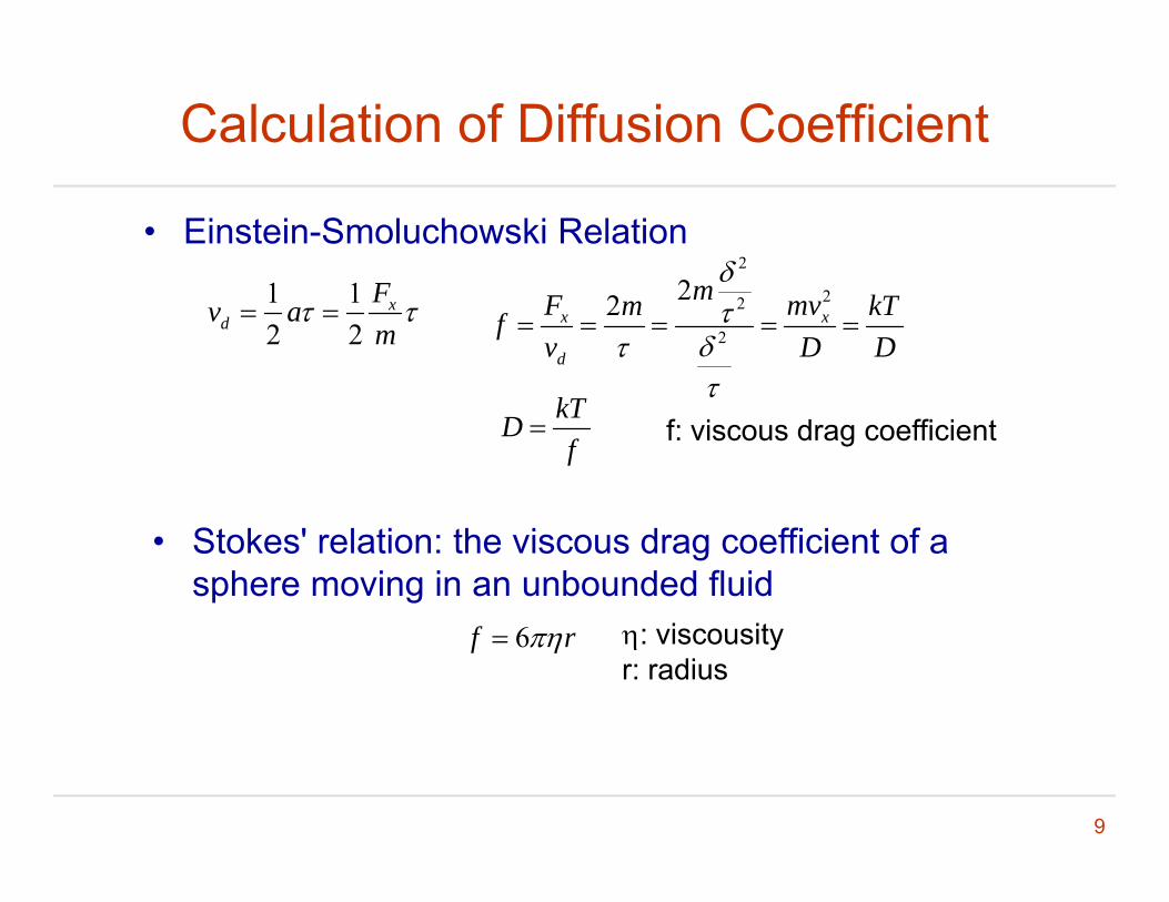
2 • Einstein-Smoluchowski Relation
1 12 2
xd
Fv am
22
2
22x x
d
mF mvm kTfv D D
kTDf
f: viscous drag coefficient
• Stokes' relation: the viscous drag coefficient of a sphere moving in an unbounded fluid
6f r : viscousityr: radius
9

An example of D calculation
• Calculation of diffusion coefficient
6kTD
r
• k=1.38110-23J/k=1.381 10-17 N·m/k• T = 273.15 + 25• =0.8904mPa·s=0.8904 10-3 10-12N·m-2·s• r= 500nm=0 5μmr 500nm 0.5μm• D=0.5 m2/s
10
Outline
• Review: polymer mechanics; Problem set 02• Review: polymer mechanics; Problem set 02
• Modeling biochemical reactionsg
• Project assignment 02
• Review: project assignment 01
11

Overview
• In general, there are two approachesg , pp- Classical approach- Contemporary approach
• The classical approach describes the steady state of biochemical reactions.
• Contemporary approach can also describes the d i f bi h i l tidynamics of biochemical reactions.
12

Modeling First Order Reactions (I)
• First order reactions involves one reactant (R).
R PR P
• Two examples
Protein conformation change Protein conformation change
Disassociation of a molecular complex
13

Modeling First Order Reactions (II)
• Forward reaction model
: d P d R
Forward k Rdt dt
• Backward reaction model :
d R d PBackward k P
• Putting together
: Backward k Pdt dt
d R
d Rk R k P
dtd P
k R k P
14
k R k Pdt

Modeling First Order Reactions (III)
• Determination of equilibrium state
k
R P
eq eqk R k P
P k k
eqeq
eq
P kKkR
15

Classic Approach to Determine 1st Order Rate Constant
• First order rate constant can be measured fromreaction half-time.
d Rk R
dt
0k t
tR R e
1/21 k tR R e 1/2
0 02R R e
1/2 2 0.6931k t ln
16

Modeling Second Order Reactions (I)
• Second order reactions involves two reactants (A,B).
• A second order molecular binding reaction
Reaction rate model
A B AB
• Reaction rate model : d P
Forward k A Bdt
d A d B : d A d B
Backward k ABdt dt
eqABkK
17
eqeq
eq eq
Kk A B

Outline
• Review: polymer mechanics; Problem set 02• Review: polymer mechanics; Problem set 02
• Modeling biochemical reactionsg
• Project assignment 02
• Review: project assignment 01
18
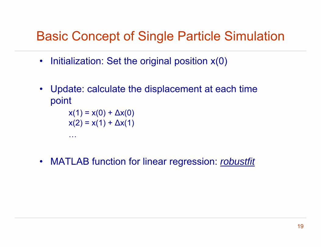
Basic Concept of Single Particle Simulation
• Initialization: Set the original position x(0)
• Update: calculate the displacement at each time point
x(1) = x(0) + ∆x(0)x(2) = x(1) + ∆x(1)…
• MATLAB function for linear regression: robustfit
19
Numerical Solution of PDE (I)
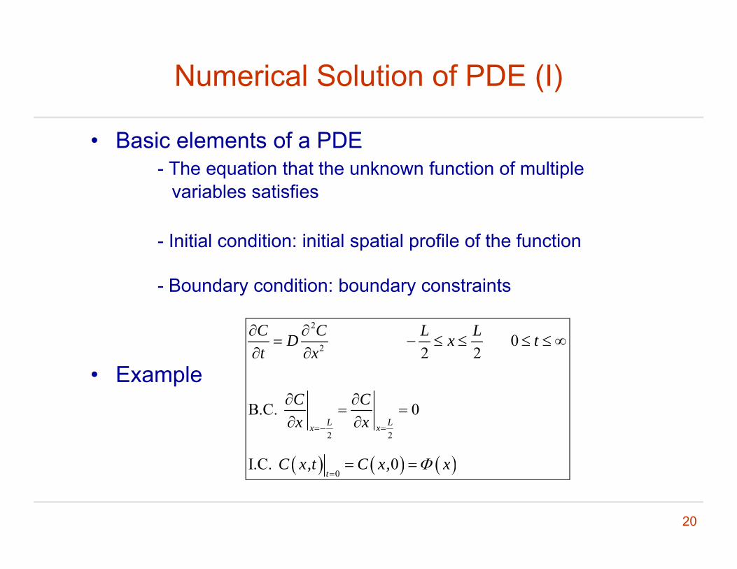
• Basic elements of a PDE- The equation that the unknown function of multiple q p
variables satisfies
- Initial condition: initial spatial profile of the functionp p
- Boundary condition: boundary constraints
• Example
2
2 02 2
C C L LD x tt x
2 2
B.C. 0
I C 0
L Lx x
C Cx x
C x t C x x
20
0
I.C. 0t
C x,t C x, x

Numerical Solution of PDE (II)
• Numerical solution of PDE
21 1
1 122
1 12n n n nj j j jn n n
j j jx j x;t n t
c c c cC c c cx x x xx
• Outline of the programfor j = 1 : M
c(j, 1) = … % this needs to be set according to initial condition; endfor n = 1 : N
for j = 2 : (M – 1)c(j, n+1) = c(j,n) + D * deltaT / deltaX / deltaX * (c(j+1, n) …
-2 * c(j, n) + c(j – 1, n));end
21
c(1, n+1) = c(2, n+1);c(M, n+1) = c(M-1, n+1);
end

Outline
• Review: polymer mechanics; Problem set 02• Review: polymer mechanics; Problem set 02
• Modeling biochemical reactionsg
• Project assignment 02
• Review: project assignment 01
22
Top Related