


![Direct construction method for conservation laws of ...bluman/EJAM2002(1).pdf · Ordinary Di erential Equations (ODEs) are given in Anco & Bluman Ref. [3]. Here we concentrate on](https://static.fdocuments.us/doc/165x107/5faabc4228aedb265a4143a8/direct-construction-method-for-conservation-laws-of-blumanejam20021pdf.jpg)
Languages
Pages
Legal


Bluman, Chapter 6 1

Review the following from
Chapter 5
A surgical procedure has an 85% chance of
success and a doctor performs the
procedure on 10 patients, find the following:
a) The probability that the procedure was
successful on exactly two patients?
b) The mean, variance and standard
deviation of number of successful surgeries.
Bluman, Chapter 6 2

Approximating a Binomial Distribution
But what if the doctor performs the surgical procedure on 150 patients and you want to find the probability of fewer than 100 successful surgeries?
To do this using the techniques described in chapter 5, you would have to use the binomial formula 100 times and find the sum of the resulting probabilities. This is not practical and a better approach is to use a normal distribution to approximate the binomial distribution.

6.4 The Normal Approximation to
the Binomial Distribution
A normal distribution is often used to solve
problems that involve the binomial distribution
since when n is large (say, 100), the calculations
are too difficult to do by hand using the binomial
distribution.
Bluman, Chapter 6 4

The Normal Approximation to the
Binomial Distribution
The normal approximation to the binomial
is appropriate when np > 5 and nq > 5 .
I. 𝝁 = 𝒏𝒑
II. 𝝈 = 𝒏𝒑𝒒 𝒘𝒉𝒆𝒓𝒆 𝒒 = 𝟏 − 𝒑
See page 274 for above formulas.
Bluman, Chapter 6 5

The Normal Approximation to the
Binomial Distribution
In addition, a correction for continuity may be
used in the normal approximation to the
binomial.
The continuity correction means that for any
specific value of X, say 8, the boundaries of X
in the binomial distribution (in this case, 7.5 to
8.5) must be used.
Bluman, Chapter 6 6

Correction for Continuity

Websites
The following websites simulate the
concept.
http://opl.apa.org/contributions/Rice/rvls_sim
/stat_sim/normal_approx/index.html
http://www.rossmanchance.com/applets/Bin
omDist/BinomDist.html
Bluman, Chapter 6 8
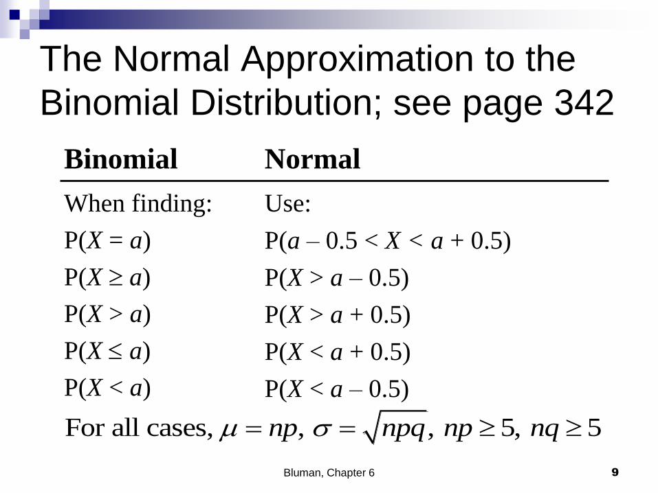
The Normal Approximation to the
Binomial Distribution; see page 342
Binomial
When finding:
P(X = a)
P(X a)
P(X > a)
P(X a)
P(X < a)
Bluman, Chapter 6 9
Normal
Use:
P(a – 0.5 < X < a + 0.5)
P(X > a – 0.5)
P(X > a + 0.5)
P(X < a + 0.5)
P(X < a – 0.5)
For all cases, , , 5, 5 np npq np nq

Bluman, Chapter 6 10

The Normal Approximation to the
Binomial Distribution
Bluman, Chapter 6 11
Procedure Table Step 1: Check to see whether the normal approximation
can be used.
Step 2: Find the mean µ and the standard deviation .
Step 3: Write the problem in probability notation, using X.
Step 4: Rewrite the problem by using the continuity
correction factor, and show the corresponding area
under the normal distribution.
Step 5: Find the corresponding z values.
Step 6: Find the solution.

Ex. 3: Approximating a Binomial Probability
Thirty-seven percent of Americans say they always fly an American flag on the Fourth of July. You randomly select 15 Americans and ask each if he or she flies an American flag on the Fourth of July. What is the probability that fewer than eight of them reply yes?
SOLUTION: From Example 1, you know that you can
use a normal distribution with = 5.55 and ≈1.87 to
approximate the binomial distribution. By applying the
continuity correction, you can rewrite the discrete
probability P(x < 8) as P (x < 7.5). The graph on the
next slide shows a normal curve with = 5.55 and
≈1.87 and a shaded area to the left of 7.5. The z-score
that corresponds to x = 7.5 is

Continued . . .
04.187.1
55.55.7
xz
Using the Standard Normal
Table,
P (z<1.04) = 0.8508
So, the probability that fewer than eight people respond yes is
0.8508

Ex. 4: Approximating a Binomial Probability
Twenty-nine percent of Americans say they are confident that passenger trips to the moon will occur during their lifetime. You randomly select 200 Americans and ask if he or she thinks passenger trips to the moon will occur in his or her lifetime. What is the probability that at least 50 will say yes?
SOLUTION: Because np = 200 ● 0.29 = 58 and nq =
200 ● 0.71 = 142, the binomial variable x is
approximately normally distributed with
58 np
42.671.029.0200 npq
and

Ex. 4 Continued
Using the correction for continuity, you can rewrite
the discrete probability P (x ≥ 50) as the
continuous probability P ( x ≥ 49.5). The graph
shows a normal curve with = 58 and = 6.42,
and a shaded area to the right of 49.5.

Ex. 4 Continued
The z-score that corresponds to 49.5 is
So, the probability that at least 50 will say yes is:
P(x ≥ 49.5) = 1 – P(z -1.32)
= 1 – 0.0934
= 0.9066
32.142.6
585.49
xz
Chapter 6
Normal Distributions
Section 6-4
Example 6-16
Page #343
Bluman, Chapter 6 17

A magazine reported that 6% of American drivers read the
newspaper while driving. If 300 drivers are selected at
random, find the probability that exactly 25 say they read
the newspaper while driving.
Here, p = 0.06, q = 0.94, and n = 300.
Step 1: Check to see whether a normal approximation can
be used.
np = (300)(0.06) = 18 and nq = (300)(0.94) = 282
Since np 5 and nq 5, we can use the normal distribution.
Step 2: Find the mean and standard deviation.
µ = np = (300)(0.06) = 18
Example 6-16: Reading While Driving
Bluman, Chapter 6 18
300 0.06 0.94 4.11 npq

Step 3: Write in probability notation.
Step 4: Rewrite using the continuity correction factor.
P(24.5 < X < 25.5)
Step 5: Find the corresponding z values.
Step 6: Find the solution
The area between the two z values is
0.9656 - 0.9429 = 0.0227, or 2.27%.
Hence, the probability that exactly 25 people read the
newspaper while driving is 2.27%.
Example 6-16: Reading While Driving
Bluman, Chapter 6 19
24.5 18 25.5 181.58, 1.82
4.11 4.11
z z
P(X = 25)

Chapter 6
Normal Distributions
Section 6-4
Example 6-17
Page #343
Bluman, Chapter 6 20

Of the members of a bowling league, 10% are widowed. If
200 bowling league members are selected at random, find
the probability that 10 or more will be widowed.
Here, p = 0.10, q = 0.90, and n = 200.
Step 1: Check to see whether a normal approximation can
be used.
np = (200)(0.10) = 20 and nq = (200)(0.90) = 180
Since np 5 and nq 5, we can use the normal distribution.
Step 2: Find the mean and standard deviation.
µ = np = (200)(0.06) = 20
Example 6-17: Widowed Bowlers
Bluman, Chapter 6 21
200 0.10 0.90 4.24 npq

Step 3: Write in probability notation.
Step 4: Rewrite using the continuity correction factor.
P(X > 9.5)
Step 5: Find the corresponding z values.
Step 6: Find the solution
The area to the right of the z value is
1.0000 - 0.0066 = 0.9934, or 99.34%.
The probability of 10 or more widowed people in a random
sample of 200 bowling league members is 99.34%.
Example 6-17: Widowed Bowlers
Bluman, Chapter 6 22
9.5 202.48
4.24
z
P(X 10)
Study Tip
In a discrete distribution, there is a
difference between P (x ≥ c) and P( x > c).
This is true because the probability that x
is exactly c is not zero. In a continuous
distribution, however, there is no
difference between P (x ≥ c) and P (x >c)
because the probability that x is exactly c
is zero.
homework
Sec 6.4 page 346
#5-13 odds
Bluman, Chapter 6 24
Top Related