


Languages
Pages
Legal


6601 2017
Original Version: August 2017
This Version: June 2018
Bismarck’s Health Insurance and the Mortality Decline Stefan Bauernschuster, Anastasia Driva, Erik Hornung

Impressum:
CESifo Working Papers ISSN 2364‐1428 (electronic version) Publisher and distributor: Munich Society for the Promotion of Economic Research ‐ CESifo GmbH The international platform of Ludwigs‐Maximilians University’s Center for Economic Studies and the ifo Institute Poschingerstr. 5, 81679 Munich, Germany Telephone +49 (0)89 2180‐2740, Telefax +49 (0)89 2180‐17845, email [email protected] Editors: Clemens Fuest, Oliver Falck, Jasmin Gröschl www.cesifo‐group.org/wp An electronic version of the paper may be downloaded ∙ from the SSRN website: www.SSRN.com ∙ from the RePEc website: www.RePEc.org ∙ from the CESifo website: www.CESifo‐group.org/wp

CESifo Working Paper No. 6601 Category 3: Social Protection
Bismarck’s Health Insurance and the Mortality Decline
Abstract
We study the impact of social health insurance on mortality. Using the introduction of compulsory health insurance in the German Empire in 1884 as a natural experiment, we estimate flexible difference-in-differences models exploiting variation in eligibility for insurance across occupations. Our findings suggest that Bismarck’s health insurance generated a significant mortality reduction. Despite the absence of antibiotics and most vaccines, we find the results to be largely driven by a decline of deaths from infectious diseases. We present evidence suggesting that the decline is associated with access to health services but not sick pay. This finding may be explained by insurance fund physicians transmitting new knowledge on infectious disease prevention.
JEL-Codes: I130, I180, N330, J110.
Keywords: health insurance, mortality, demographic transition, Prussia:
Stefan Bauernschuster University of Passau
Germany – 94032 Passau [email protected]
Anastasia Driva
LMU Munich Germany – 80539 Munich
Erik Hornung
University of Cologne Germany – 50923 Cologne [email protected]
This version: June 2018 We thank Andrew Goodman-Bacon, Leah Platt Boustan, Davide Cantoni, Francesco Cinnirella, Greg Clark, Dora Costa, Carl-Johan Dalgaard, Katherine Eriksson, Oliver Falck, James Fenske, Price Fishback, Michael Grimm, Casper Worm Hansen, Walker Hanlon, Timo Hener, Adriana Lleras-Muney, Chris Meissner, John E. Murray, Jochen Streb, Uwe Sunde, Joachim Voth, Till vonWachter, Joachim Winter, Ludger Wößmann and seminar participants at Arizona, Bayreuth, Copenhagen, Deutsche Bundesbank, DIW Berlin, Frankfurt, Göttingen, Hohenheim, Innsbruck, the Ifo Institute, ISER, IZA, Lausanne, Linz, LMU Munich, Maastricht, MPI for Tax Law and Public Finance, Southern California Population Research Center, Passau, Potsdam, Trier, UC Davis, UC Berkeley, UCLA, Zurich, the 2015 FRESH Meeting in Barcelona, the 2016 Workshop Culture, Institutions and Development in Galatina, the 2016 Workshop Markets and States in History at Warwick, the 2016 meeting of the EHA in Boulder, the 2017 Congress of Economic and Social History in Bonn, and the 2017 Workshop on Health Economics and Health Policy in Heidelberg. This work was financially supported by an Arthur H. Cole Grant awarded by the Economic History Association in 2015. Driva gratefully acknowledges the hospitality provided during a research visit at UCLA as well as the funding through the International Doctoral Program “Evidence-Based Economics” of the Elite Network of Bavaria. We are grateful to our research assistants Tamara Bogatzki, Carolin Fries, Leonie Kirchhoff, Sigfried Klein, Hannah Lachenmaier, Max Neumann, Philipp Nickol, and Markus Urbauer.

“Rarely, if ever, in modern history has a single piece of legislation hadsuch a profound worldwide impact as the German Sickness Insurance Law of1883 - the cornerstone of German health care policy for almost one century.”
– Leichter (1979)
1 Introduction
From the mid of the 19th century, the industrializing world experienced an unprecedented
decline in mortality rates. This mortality reduction is central to the demographic transi-
tion and had arguably fundamental consequences for long-run growth and productivity.1
An ongoing debate is concerned with the forces contributing to the mortality decline.
Most major advances in medicine such as antibiotics and vaccines did not occur before the
1930s and were not decisive for the considerable reduction of infectious disease mortality
during the early phase of the health transition. A large literature discusses the influence
of improvements in income and nutrition, directed investments in public sanitation, and
scientific advances in health knowledge.2 Yet, this literature has mostly neglected the
emergence of social health insurance at the end of the 19th century.
This paper investigates the impact of Bismarck’s health insurance on mortality
in Prussia. As Chancellor of the German Empire, Otto von Bismarck introduced the first-
ever widely-implemented compulsory health insurance in the world in 1884. Covering large
parts of the working population, Bismarck’s health insurance (henceforth BHI) was a first
move toward democratized access to health care. Subsequently, it acted as a blueprint
for Germany’s current health system and served as a model for many social insurance
systems across the world. Surprisingly however, econometric studies on the health effects
of BHI have been missing so far.
Our main empirical approach exploits the fact that BHI became compulsory
only for the blue collar worker population while other occupations’ access to health care
remained unchanged. Newly digitized administrative data from Prussia, the largest of the
German states when BHI was introduced, allow us to compute annual occupation-specific
mortality rates at the district level for the period 1877 to 1900. We bring these unique
panel data to a generalized difference-in-differences model that compares the mortality
trend of blue collar workers (treatment group) to the mortality trend of public servants
(control group) while allowing for heterogenous reform effects over time.
Difference-in-differences estimates indicate that, from its introduction in 1884
to the turn of the century, BHI reduced blue collar workers’ mortality by 8.9 percent.
Thus, the insurance accounts for roughly a third of the total mortality decline of blue-
collar workers during this period. The results are robust to allowing for heterogeneous
effects of urbanization, the establishment of waterworks, and the roll-out of sewerage.
1While microeconomic evidence typically confirms the existence of health-induced productivity gains, the rela-tionship between improvements in health and aggregate productivity is subject to ongoing debate. Many studiesfocus on specific periods of major improvements in health and life expectancy to test this relationship (for some im-portant contributions, see Acemoglu and Johnson, 2007; Ashraf et al., 2008; Bleakley, 2007; Hansen and Lønstrup,2015; Jayachandran and Lleras-Muney, 2009; Lorentzen et al., 2008; Murtin, 2013; Weil, 2007, 2014).
2Seminal contributions include, e.g. Cutler and Miller (2005), Deaton (2013), McKeown (1979), Fogel (2004),and Preston (1975). For recent surveys see Costa (2015) and Cutler et al. (2006).
1

Common pre-treatment mortality trends across occupations corroborate the validity of
the identification strategy. Additionally, we find that BHI created substantial spillovers
from the insured to their uninsured family members. The results are neither confounded
by contemporaneous social reforms nor by improved working conditions or increasing
wages for blue-collar workers.
A range of additional econometric approaches provide corroborating evidence for
the effects of Bismarck’s health insurance. These various approaches yield a consistent
pattern suggesting negative effects of BHI on mortality. To address concerns regarding
potential selection into the industrial sector after the introduction of BHI, we employ
county- and district-fixed effects models that exploit regional differences in the blue-collar
workers share fixed at a point in time before the introduction of BHI. The fixed effects
models also allow us to rigorously control for changes in the population age structure, to
account for the strength of unions, and to perform a specification test using a placebo
treatment group. To understand whether Prussia’s mortality reduction was particularly
pronounced, we employ country-level time series data that allow analyzing the decline in
international comparison. While mortality decreased in all Western European countries
toward the end of the 19th century, we find that the introduction of BHI indeed coincides
with the beginning of a more accentuated drop in Prussian mortality.
We shed light on the channels through which BHI contributed to the mortality
decline by inspecting heterogeneity in the causes of death and by comparing the effective-
ness of insurance benefits. Using newly digitized data on causes of death in a district fixed
effects framework, we show that a large part of the decline results from a reduction of
mortality due to airborne infectious diseases. Especially tuberculosis, a disease for which
a cure was not developed until 1946, declined in response to BHI. Further results, based
on insurance benefits, indicate that a substantial share of deaths were avoided due to
individual interactions with physicians and medical treatment but not via sick pay, the
main expense of insurance funds. This finding lends support to the view that diffusion
of new health knowledge became relevant for public health before the turn of the 20th
century.
We interpret the findings to imply that BHI was instrumental in extending access
to doctors who acted as transmitters of health knowledge to poor working class families,
a group formerly unable or unwilling to afford health care. This hypothesis complements
earlier conjectures in the historical literature arguing that the insurance provided its
members with access to new knowledge regarding hygiene and transmission of infectious
diseases (see Condrau, 2000; Koch, 1901; Vogele, 1998). Our claim resonates with the
approach of Mokyr and Stein (1996) who build a model of consumer behavior in which
households produce health for its members based on the existing priors on the causes of
disease. These priors were radically altered by the germ theory of disease at the end of
the 19th century when inputs to the health production function substantially changed.
In order for scientific knowledge to affect household priors, a vehicle of transmission
is crucial. Indeed, sickness funds encouraged their licensed physicians to disseminate
the newly gained knowledge of infectious disease transmission and launched information
campaigns to facilitate the application of hygiene knowledge. We provide support for this
interpretation by presenting evidence on heterogenous effects of insurance benefits. While
fund’s expenditures for doctor visits and medication are negatively related to mortality
2

in a district fixed effects model, expenditures for sick pay are not. These findings lend
prima facie support to the view that the insurance improved health by providing access
to health care rather than by providing sick pay.
More recent expansions of compulsory health insurance have been highly effective
in increasing access to health care and reducing mortality, at least for specific subgroups of
the population. In this respect, our findings are in line with studies on major expansions
in health insurance coverage in the U.S., such as Medicare for the elderly (see Card et
al., 2008, 2009; Finkelstein, 2007; Finkelstein and McKnight, 2008) and Medicaid for the
poor (see Currie and Gruber, 1996; Goodman-Bacon, 2017). Yet, there are some key
differences between these 20th century expansions and the introduction of BHI. Present-
day health insurance schemes work in an environment of chronic diseases and benefit
from the ability to provide health care by medical treatment. In contrast, BHI was
established in an environment of infectious diseases whose treatment had not sufficiently
developed. As such, our setting might be more readily comparable to the situation in
developing countries, where an increasing number of compulsory health insurance schemes
are currently introduced (Lagomarsino et al., 2012; Malik, 2014). These schemes are
introduced in an environment with a high prevalence of infectious diseases with large
parts of the population lacking adequate knowledge on hygiene and disease transmission.
The remainder of the paper is organized as follows. Chapter 2 discusses the
literature on the causes of 19th century’s mortality decline and provides background
information on Bismarck’s health insurance. Chapter 3 introduces the historical Prussian
district-level data that we use in the empirical analysis. Chapter 4 presents the multiple
empirical approaches, presents the results and provides a set of robustness and validity
checks. Chapter 5 concludes.
2 Literature and institutional background
2.1 Literature on the causes of the mortality decline
Germany’s mortality and fertility decline at the end of the 19th century is considered
to be fairly representative of the demographic transition in many European countries
(Guinnane, 2011). Yet, Germany experienced higher levels of mortality and fertility than
most other European countries at the beginning of the 19th century. With respect to
mortality, Leonard and Ljungberg (2010) depict a ‘German penalty’ which was evident in
1870, but vanished by 1900 when Germany’s mortality had declined to the levels of other
countries. In the period 1875 to 1905, life expectancy of a German child below the age of
one increased from 38.4 to 45.5; for individuals between the age of 20 and 25 it increased
from 43.2 to 47.8 (Imhof, 1994). Life expectancy in rural areas of Europe was considerably
higher than in urban areas until the beginning of the 20th century (e.g., Kesztenbaum and
Rosenthal, 2011). At birth, the average Prussian boy living in the countryside expected
to outlive his urban counterpart by five years (Vogele, 1998).
The precise factors that contributed to the mortality decline remain disputed.
The empirical literature has attempted to provide various explanations, ranging from nu-
tritional improvements and public investments in sanitation infrastructure to the diffusion
3

of knowledge as a tool to prevent disease transmission. Seminal contributions by McKe-
own (1979) and Fogel (2004) argue that improvements in living standards and nutrition
were responsible for the mortality decline in 19th century Europe, ruling out many other
factors. The role of public health measures was first revised by Szreter (1988). In contrast
to the views of McKeown (1979) and Fogel (2004), the literature broadly agrees that espe-
cially the ‘urban penalty’ was gradually removed through a range of investments in public
sanitation infrastructure during the second half of the 19th century. Many recent studies
provide evidence for major reductions in infant and adult mortality which are associated
with improvements in sanitation infrastructure (Hennock, 2000; Meeker, 1974). More
specifically, improvements in the water supply (Brown, 1988; Ferrie and Troesken, 2008;
Beach et al., 2016), water purification (Cutler and Miller, 2005), and sewerage systems
(Alsan and Goldin, 2015; Kesztenbaum and Rosenthal, 2017) strongly reduced mortality
from waterborne diseases.
Cutler et al. (2006) and Leonard and Ljungberg (2010) argue that medical treat-
ments hardly contributed to the mortality decline before 1914. However, effective medica-
tion was not entirely absent at that time. Indeed, smallpox vaccination became available
already in 1796 and largely reduced infant mortality (Ager et al., 2017; Hennock, 1998).
In the first decades of the 19th century, many German states introduced compulsory
vaccination against smallpox. While this was not true for Prussia, smallpox vaccination
and re-vaccination were a widespread practice and eventually became compulsory for all
children as part of the Imperial German Vaccination Law in 1874. In 1885, rabies vaccine
became available. In 1891, the first drugs against diphtheria emerged. A range of antisep-
tics and anesthetics were widely used. More generally, the end of the 19th century saw a
significant progress in chemistry that allowed identifying effective ingredients of medicinal
plants and producing new chemical drugs.
The medical sector expanded substantially at the end of the 19th century. From
1870 to 1890, the number of medical students in Prussian universities more than tripled
(from 2,600 to 8,724), whereas the number of students of all other faculties roughly dou-
bled. As a result, by 1890, the medical faculty boasted the largest number of students of
all faculties. Similarly, data from the Prussian occupation censuses show that the share
of people working in the health sector grew by about 40 percent from 1882 to 1907.
Overall, scientific medical knowledge deepened considerably towards the turn of
the century (Mokyr and Stein, 1996). The widely held belief, prevalent since medieval
times, that diseases were transmitted through bad smells (miasmas) gradually faded out
during the course of the 19th century. It was replaced by scientific findings identifying
the role of bacteria as crucial transmitters of diseases. Major breakthroughs in epidemiol-
ogy and bacteriology occurred during the second half of the 19th century (for details see
Easterlin, 1999). These included the well-known discoveries of water as a transmitter of
Cholera by John Snow and William Budd as well as numerous discoveries in bacteriology
by Robert Koch, Louis Pasteur, Ignaz Semmelweis and others.3 Advances in bacteri-
ology had an impact on established knowledge across all types of infections related to
3The role of hygiene, as an important tool to prevent infectious diseases in hospitals, became generally appre-ciated in the 1880s, twenty years after the death of Ignaz Semmelweis, the pioneer of modern antisepsis (Murken,1983). Yet, it was not before Alexander Fleming discovered penicillin in 1928 that antibiotics became widely knownas drugs that could fight bacteria.
4

waterborne and airborne diseases. In fact, Mokyr (2000, p. 15) recognizes germ theory to
be “one of the most significant technological breakthroughs in history.” However, mere
identification of the root cause of infections was insufficient to cure the sick, especially
when no remedies were available. All that physicians could do was to “educate patients
on hygiene” (Thomasson, 2013, p. 177).
The role of knowledge diffusion in improving health has recently gained the at-
tention of economists. Deaton (2013), for instance, argues that upward shifts of the
Preston curve are driven by the application of new knowledge. In the first half of the
20th century, knowledge regarding hygiene was disseminated via health care centers, con-
gresses and public information events around the developed world. Nordic countries were
particularly progressive in diffusing knowledge through well-child visits and health care
centers. Wust (2012) finds that Danish infant mortality was reduced due to home visiting
programs which helped towards diffusing knowledge on nutrition as well as highlighting
the positive health effects of breastfeeding. Bhalotra et al. (2017) show that a similar
Swedish program managed to reduce chronic diseases of infants by providing nutritional
information, non-financial support and monitoring. According to findings by Butikofer et
al. (forthcoming), Norwegian mother-child health care centers also contributed to better
long-term economic outcomes by granting universal and free access to well-child visits
during the first year of life. Ogasawara and Kobayashi (2015) find similar effects when
evaluating a program for inter-war Tokyo. Hansen et al. (2016) investigate the introduc-
tion of tuberculosis dispensaries in Denmark in the early 20th century. In the absence of
a cure, these dispensaries disseminated knowledge related to the transmission of tubercu-
losis to patients and their families as well as to the general public significantly decreasing
tuberculosis mortality.4
Public interventions also include the introduction of health insurance across Eu-
ropean countries at the turn of the 20th century. According to Vogele (1998), health
insurance funds might have contributed to the penetration of new knowledge and health
education in the German Empire.5 Guinnane (2003, p. 45) supports this hypothesis by
noting that the insurance sickness funds played a major role in strengthening the role
of physicians as advocates of hygiene. Kintner (1985) argues that physicians and mid-
wives represented a major source for disseminating information on the health effects of
breastfeeding to pregnant women.6 In addition, Tennstedt (1983, p. 461) suggests that
insurance funds fostered prevention of illness transmission by introducing new rules and
benefits for workers’ families, workers’ hygiene and lifestyle, the workplace, and the em-
ployers’ responsibilities. Yet, empirical evidence for the role of early health insurance
programs for the mortality decline is still scarce.
4Condran and Crimmins-Gardner (1978) argue that ’similar’ information campaigns in U.S. cities at the end ofthe 19th century played a minor role in reducing tuberculosis-driven mortality.
5Vogele (1998, p. 199-208) lists a range of potential channels through which BHI might have been able to increasehealth, including preventing families to fall into poverty due to sick pay, increasing access to doctors and hospitals,or by allowing the state to systematically educate and control the covered population with respect to their attentionto health issues.
6According to Kintner (1985) and Kintner (1987), breastfeeding was more widespread in Prussia compared tothe south of Germany; whereas some cities such as Baden or Munich saw an increase in breastfeeding, breastfeedingin the capital Berlin massively declined between 1885 and 1910. However, unfortunately, comprehensive data onbreastfeeding are missing before 1910. It has been argued that improvements in the quality and supply of cow milkwere only marginal in improving infant mortality conditions (Vogele, 1998). Legal regulations regarding the qualityof milk did not become an issue in the German Empire until 1901.
5

Winegarden and Murray (1998) provide empirical evidence that health insurance
coverage across five European countries was associated with mortality reductions in the
periods before World War I. They find that a ten percentage point increase in the insured
population results in a mortality reduction of 0.9 to 1.6 per 1,000 people. Bowblis (2010)
extends this study to eleven countries and studies the effect of health insurance on infant
mortality. He speculates that health insurance reduced mortality by “educating people
about the benefits of clean houses, not re-using dirty bath water, washing hands, and
isolation of sick family members from the rest of the household” (Bowblis, 2010, p. 223).
Finally, Strittmatter and Sunde (2013) show that the reduction in mortality due to the
introduction of public health care systems across Europe translates into positive effects
on growth in income per capita and aggregate income. Their cross-country analysis is
based on data from twelve European countries; due to a lack of data availability, they
exclude Germany, the country which introduced the first public health insurance system
and boasts the largest share of insured at the turn of the 19th century. These stud-
ies provide an interesting yardstick for our findings. Yet, while all three studies exploit
across-country, over-time variation, our empirical setup exploits within-country, over-time,
across-occupation variation. This setup allows us to flexibly control for general mortal-
ity trends within the country and time-invariant factors that are specific to subregions.
Moreover, we contribute to this literature by taking several steps to explore the potential
channels of the mortality effects using newly digitized administrative data from Prussia.
2.2 Bismarck’s health insurance
The Compulsory Health Insurance Act of 1883 constituted the birth of Germany’s social
security system. Bismarck’s health insurance was the first of the three main branches of
the German Social Insurance System, followed by the Accident Insurance Act (1884) and
the Disability/Old-age Pension System Act (1891).7
Chancellor Otto von Bismarck’s decision to introduce the compulsory health in-
surance was a reluctant reaction to mounting upheavals among the working class. The
Industrial Revolution led to increasing social tension between the rising working class and
the political and economic elite. The new Socialist Workers Party of Germany gained
support among the lower strata of the population and became a threat to the political
stability of conservative dominance in the German Reich Parliament. Against this back-
drop, the health insurance reform was a mass bribery for Bismarck to win over votes from
the socialist party and the worker unions (Rosenberg, 1967). Furthermore, it disburdened
public funds by shifting the cost of poor relief to workers and employers. The Reichstag
approved the law on May 31, 1883, against the votes of the Social Democrats who argued
that this social reform would not really improve the workers’ situation (Tennstedt, 1983).
From December 1st, 1884, BHI was “compulsory for all industrial wage earners
(i.e. manual laborers) in factories, ironworks, mines, ship-building yards and similar
workplaces” (Act of June 15, 1883, see Leichter, 1979). Contributions were earnings-
7Scheubel (2013) provides an excellent overview of Bismarck’s social security system. Fenge and Scheubel (2017)show that the introduction of the disability and old age pension system reduced fertility, while Guinnane and Streb(2011) provide evidence for moral hazard effects of the accidence insurance. Lehmann-Hasemeyer and Streb (2016)find that Bismarck’s social security system as a whole crowded out private savings.
6

related, amounted to an average of 1.5 percent of the wage8 and were paid jointly by
employers (one-third) and employees (two-thirds). Other occupations, including public
servants, farmers, domestic servants, day-laborers or self-employed were not eligible for
BHI.
In case of sickness, the insured were eligible to receive sick pay amounting to at
least 50 percent of the average local wage for 13 weeks. Moreover, funds were allowed to
extend free health care to family members. Note that the Act only specified maximum
contributions and minimum benefits. Thus, the individual sickness funds had “consider-
able discretion to set specific benefits and contribution levels” (Leichter, 1979, p. 123).
Further benefits included free routine medical and dental care, prescribed medicine, inci-
dental care for up to 13 weeks and treatment in hospitals for up to 26 weeks. In addition,
the insurance provided maternity benefits encompassing free medical attention and a cash
benefit (Wochenhilfe) for three weeks after giving birth. In case of death of an insured
worker, the insurance paid a death grant to the worker’s family.
The health insurance system was administered in a decentralized manner by lo-
cal sickness funds (Krankenkassen). Generally, we can distinguish between six types of
sickness funds. Where possible, Bismarck built upon previously existing organizations
such as the building trade, the miners (Knappschaften), the guild and various indus-
trial sickness funds.9 This saved both time and state resources and was sensible from
a political perspective because it respected the guilds’ and unions’ position as insurance
providers for their members. In addition to these four types of funds, two new types were
established: these included the local funds (Ortskrankenkassen) and the parish funds
(Gemeindekrankenkassen) whose task was to insure all eligible workers not covered by
other funds. These two new funds attracted the lion’s share of the newly insured workers
after the 1884 reform. Indeed, 59 percent of all insured individuals were insured in either
local or parish funds by 1905.
After issuing the Act in 1883, municipalities and other institutions had more
than a year of preparatory time to set up the insurance funds. Yet, the very early period
of BHI did not pass without frictions. Employers did not report their workers to the
funds, workers opted to remain in pre-existing funds with lower benefits, and collectors
of insurance premia returned drunk and lost their lists.10 The literature typically argues
that workers were unenthusiastic about the insurance and concerned about employer’s
resentments regarding their share of contributions. As a result, some workers preferred to
buy insurance from voluntary funds (Hilfskassen) that did not require employer contri-
butions and employers preferred to hire workers with such insurances (Tennstedt, 1983,
pp. 318-322). Initially, around 40 percent of the targeted workers took up insurance. In
the following years, this share gradually increased, also due to more rigorous inspection.
8Contributions were confined to a maximum range of 3 to 6 percent of the wage.9Only few workers from minor industries were covered by these particular insurance funds; most of them were
members of the Knappschaften which provided insurance against accident, illness, and old age from 1854 (see alsoGuinnane and Streb, 2011).
10Based on the occupation census of 1882, officials in Dresden were expecting 45,000 workers from 8,665 firms tobe liable for compulsory insurance. By mid 1885, only 30,000 workers were registered and 3,000 employers had yetto report their workers. Similar compliance rates were reported from Leipzig (Tennstedt, 1983, p.319).
7

Figure 1 depicts the development of health insurance coverage over time.11 Pre-
1885 insured are either voluntarily insured or clustered in very few small industries provid-
ing compulsory health insurance such as mining. The data suggest only slight increases in
the insured population until 1876, the latest available pre-BHI data point, after which the
insured population surged from 3 percent to 8 percent in 1885. The subsequent increase
in insured population is likely due to several reasons, including the increased uptake after
initial frictions in recording the eligible workers, an expansion in the blue collar worker
population due to ongoing industrialization, and a stepwise extension of BHI towards
white collar groups (Angestellte). The steady increase in the share of insured after 1885
suggests that any effects of BHI are likely to become stronger over time.
Historical accounts suggest that being covered by BHI increased the demand
for health goods and services. The insured consulted physicians far earlier and more
frequently than the uninsured and it is argued that a large share of the newly insured would
not have been able to afford consulting a physician in the absence of BHI (Huerkamp,
1985, p. 202).12 The insured were in fact legally required to consult a licensed physician
to receive a sick note and become eligible for sick pay. Fund physicians often received a
lump sum payment of 2 Marks per insured from the insurance funds, irrespective of the
treatment frequency. Since the insured did not bear the immediate costs, they increasingly
made use of consultation hours. The stereotypical doctor’s complaint that patients came
for consultation only when it was too late turned into complaints that patients came in
for petty indispositions (Huerkamp, 1985, p. 201).13 Moreover, BHI became a key driver
of the increased utilization of hospital capacity in the 1890s (Spree, 1996). Vogele et al.
(1996) find that half of the patients in Dusseldorf hospitals were compulsory insured by
1901. The majority of inpatients were treated for non-communicable skin, eye and surgical
diseases, i.e. treatment of injuries and wounds. Technological progress in antiseptics and
improved sterilizing of wounds was highly supportive for successful treatment.
Contemporary complaints typically criticized the insurance’s main benefit – sick
pay. In principle, sick pay constitutes an improvement to the previous situation in which
workers received no income while being sick at home. However, workers were hardly able
to subsist on half of the local daily wage and the historical accounts suggest that they
preferred returning to work as soon as possible (Ellerkamp, 1991). From a political per-
spective, contemporary supporters of BHI argued that the reform was costly but “bought
social peace for Germany” (Leichter, 1979, p. 124).
3 Data
To quantify the impact of BHI on mortality, we draw on unique administrative data from
Prussia, the largest state of the German Empire. In 1885, Prussia’s territory covered
roughly two thirds of the total area and population of the German Empire. The Royal
Prussian Statistical Office is unique in having published annual death statistics by occupa-
11Table A1 in the Appendix shows the exact numbers of insured and total population of Prussia over the years.12The chairman of the Imperial Insurance Agency Tonio Bodiker argued that less than half of the worker’s families
would have consulted a doctor before the introduction of the compulsory insurance (Huerkamp, 1985, pp.207-208).13This notion is supported by contemporary sources suggesting that only half of the consultations justified a
period of sick leave (Huerkamp, 1985, pp.202).
8

tional group. We combine these data with Prussian population and occupation censuses.
The resulting data set is additionally extended to include information on public sanitation
infrastructure such as waterworks and sewerage. When further refining our analysis, we
draw on heterogeneity in the causes of death and in sickfunds’ expenditures to provide
evidence on potential channels through which the reform affected mortality. The period
of observation for the main analysis covers the years from 1875 to 1905.
3.1 Data on mortality by occupation
The Preussische Statistik (KSBB, 1861-1934), a series of statistical volumes published by
the Royal Prussian Statistical Office, annually reports the number of deaths by occupation
for all 36 Prussian districts.14 This information is reported for 28 occupational groups
from 1877. Deaths are reported for adult men and women, as well as for male and female
children below fourteen years of age. Children and non-employed females are classified by
the occupation of their father or husband, respectively. We extract eighteen occupations
that are consistently reported over time, following the classification of the Prussian Statis-
tical Office into blue collar sector and public sector.15 This categorization is particularly
helpful for our analysis since it allows to compare mortality across occupational groups
that differ in their eligibility for Bismarck’s health insurance.
The death statistics are supplemented by occupation censuses that were exclu-
sively conducted in the years 1882, 1895, and 1907 under the supervision of the Imperial
Statistical Office (KSA, 1884-1942). The period under analysis is a period of rapid indus-
trialization in Germany.16 Accordingly, the occupational groups experienced differences in
the growth of the working population leading to differences in the growth of the population
at risk (see Table 1 for details). To take this into account, we generate occupation-specific
mortality rates by combining the occupation-specific death statistics and the occupation-
specific population data from the occupation censuses. We were able to consistently
match the eighteen occupations extracted from the death statistics to those reported in
the occupation census. Gaps between census years were filled by linear interpolation and
extrapolation to obtain estimates of the respective size of each occupational group.17
14In the Prussian administrative hierarchy the district (Regierungsbezirk) ranks above the county (Landkreis).15Blue collar worker industries encompass thirteen groups listed as sector B in the statistics: mining and turf,
minerals, metals, machinery, chemicals, fossil fuels, textiles, paper and leather, wood, food, apparel and cleaning,construction, and printing. Public servant groups encompass five categories listed as sector E in the statistics:public administration, military, church and education, health, and arts and entertainment.
16Note that this period is not a period of substantial warfare. The Franco-Prussian war of 1871 did not affectPrussian territory and civilians. The war created 30,000 veterans suffering from long-term disabilities and/ordiseases. Even so, there is no evidence for the year 1884 constituting a crucial turning point in veteran’s mortality.
17Different from the death statistics, the occupation censuses report occupation-specific numbers of working malesand females but aggregate non-working family members into a single category. Thus, when calculating occupation-specific mortality rates we rely on the total occupational population (excluding servants). We tested the robustnessof our results to replacing this denominator by the occupation- and gender-specific working population. The resultsare qualitatively similar. We further tested interpolation based on urban population growth, which does not requirelinear extrapolation to years prior 1882. Again, the results are qualitatively similar.
9

3.2 Data on aggregate mortality, causes of death, and health insurancecontributors
In a range of specifications we draw on aggregate mortality rates for the period from
1875 to 1904 instead of using occupation specific mortality rates. These mortality rates
are provided by Galloway (2007) for all Prussian counties. Due to the fact that several
counties were split during administrative reforms, we aggregate the data to consistently
reflect the borders of 1875, resulting in a constant set of 441 counties. When necessary,
the data are aggregated to reflect the district level with 36 observations. Next to total
mortality, the data include gender-specific mortality and infant mortality by legitimacy
status.18
To gain insights into potential mechanisms through which BHI affected health,
we digitized rich data on the causes of death from the Preussische Statistik (KSBB, 1861-
1934). In particular, we draw on district-level information reporting the full universe of
fatalities by the thirty distinct causes of death that were reported annually from 1875
to 1904. This wealth of data allows us, for example, to distinguish between deaths from
waterborne infectious diseases such as typhus, typhoid fever, or diarrhea, and deaths
from airborne infectious diseases such as smallpox, scarlet fever, measles, diphtheria,
pertussis, scrofula, tuberculosis, tracheitis, or pneumonia. Besides, the data provides us
with information on the number of deaths due to accidents, maternal deaths and deaths
from non-infectious diseases such as cancer, edema, stroke, heart disease, brain disease,
and kidney disease.19
In specifications with aggregate or cause-specific mortality as dependent variables
we use the aggregate pre-BHI blue collar worker share as main explanatory variable. We
calculate the county- and district-specific population share employed in blue collar occupa-
tions using the above mentioned occupation census of 1882. In an alternative specification,
we draw on data recording the actual take-up of health insurance. KSA, 1884-1942 pro-
vides annual district-level records on the number of health insurance contributors, which
allows us to calculate the share of insured in the total population.20
3.3 Data on sanitation infrastructure, urbanization, age structure, andSPD vote shares
We address concerns regarding changes specific to the urban environment coinciding with
the introduction of the health insurance by supplementing our dataset with information
18We follow the standard approach to calculate crude death rates as the total number of deaths per year per1,000 people. Infant mortality is defined as the number of deaths of children below the age of one per year per1,000 live births. This applies for legitimate and illegitimate deaths and live-births respectively.
19Concerns regarding the quality of causes of death data from this period have been raised in the literature(Kintner, 1999; Lee et al., 2007). Note that it is possible that improved knowledge about diseases allowed registrarsto better identify the accurate cause of death over the course of our period of observation. If regions with a highershare of insured were also regions were physicians or registrars were better able to identify the cause of death, weexpect the residual category ‘unknown cause of death’ to show a stronger decline. Using ‘unknown cause of death’as an outcome in a district fixed effects model similar to Equation 2, we do not find evidence of such a pattern (seealso Table 6 below). This finding indicates that there were no systematic improvements in the ability to identifythe correct cause of death related to the introduction of BHI that could drive our findings on causes of death.
20Although this data is available for the entire German Empire, we confine our analysis to Prussia since ourdetailed mortality data are only available for the Prussian territory.
10

on sanitation infrastructure as well as urbanization rates. The literature discusses two
drivers of change in urban mortality occurring at the end of the 19th century which are
related to the provision of public sanitation infrastructure — waterworks and sewerage.
We draw on Grahn (1898-1902) and Salomon (1906-1907) who report city level dates of
the establishment of public water supply and sewerage systems respectively. Assuming
that the entire city population benefited from the introduction of sanitation infrastructure,
we calculate the county/district level share of the total urban population with access to
waterworks and sewerage. The Prussian Statistical Office conducted population censuses
including urban population counts every five years. These data, available from (Galloway,
2007), are linearly interpolated to generate annual estimates of the urban population and
urbanization rates.21 Depending on the specification, we are able to use county level data
or aggregate the data to the district level.
Moreover, we digitized district-level data from population censuses reported in
KSBB, 1861-1934 to generate variables that depict the age structure of the population
during the period 1875 to 1904. In particular, we calculate the average age and the
size of age cohorts (ages: 1-9, 10-19, 20-29, 30-39, 40-49, 50-59, 60-69, 70 plus) as a
fraction of the total population. These variables should capture changes in a district’s age
composition over time. Additional robustness checks rely on data from Galloway (2007)
to calculate the district-level vote share of the workers party SPD (and its predecessors)
in the general elections of 1874, 1878, 1884, 1890, 1893 and 1898 to proxy changes in the
regional strength of workers’ movements and unions.22
3.4 Data on health insurance fund expenditures, hospitalizations andlicensed physicians
In an attempt to present further prima facie evidence on the mechanisms at work, we draw
on newly digitized annual data on the expenditures of insurance funds for the period from
1885 to 1904. KSA, 1884-1942 reports district-level data from insurance funds balance
sheets. Expenditures include categories such as sick pay, medication, hospitalizations,
doctor visits, death benefits, maternity benefits and administration reported in German
Mark, as well as the number of sick days. Combining these data with the annual number
of insured in a district, we calculate per capita expenditures by type.
To conduct complimentary analyses of the demand for health services, we digi-
tized district level hospitalization rates based on the annual number of treated patients
and individual cases, reported in KSBB, 1861-1934 for the period from 1880 to 1904. To
capture the development of the supply side, we digitized district-level information on the
number of licensed physicians (approbierte Arzte) for the years 1879, 1882, 1887, 1898,
and 1901 (KSB HB, 1903).
21The waterworks data is additionally extrapolated to cover the post 1898 period.22These elections were chosen because they precede the first year of each five year interval to which we aggregate.
11

4 Empirical evidence
This section analyzes the impact of BHI on mortality using multiple empirical approaches.
Bringing together evidence from various data sets with varying degrees of aggregation,
we sequentially address a range of concerns regarding a causal interpretation of our find-
ings of BHI on mortality. The sequence of specifications starts with a comparison of
mortality trends across countries. To avoid problems of unobserved time-varying hetero-
geneity across countries, we proceed with a disaggregated intention-to-treat difference-
in-differences approach that focuses on Prussia. This approach exploits the fact that
BHI was compulsory for blue collar workers but not for other occupations and compares
occupation-specific changes in mortality rates over time. In regional fixed effects anal-
yses, we address selection issues exploiting pre-BHI variation in treatment eligibility at
the district and county level, and provide further support against confounding factors.
Finally, to explore the potential channels through which BHI affected mortality, we draw
on causes of death statistics and sickness funds’ expenditures data. Each subsection is
structured to first establish the econometric specification, then present the results and
finally discuss advantages, concerns and drawbacks particular to the respective approach.
4.1 Time-series and cross-country statistics
We start our empirical analysis by inspecting the long-run development of mortality in
Prussia from the early 19th to the early 20th century. Figure 2 plots the crude death
rate, defined as the number of deaths per 1,000 inhabitants of Prussia over the period
from 1815 to 1913. Mortality was rather volatile, due to higher prevalence of epidemics
and war, until the early 1870s when the fluctuations notably ceased. However, it is not
before the mid-1880s that we observe a distinct break in the long-run mortality trend.
From 1885 to 1913, the crude death rate in Prussia declined from about 27 to about 17
deaths per 1,000 population, corresponding to a substantial drop of almost 40 percent.
Thus, we observe a remarkable coincidence of the introduction of BHI in December 1884
with the timing of the mortality decline.
At the end of the 19th century, mortality rates declined across all industrializing
countries. Yet, the drop of German mortality rates from 1884 onwards was noticeably
more accentuated than in other Western countries, which might be related to the intro-
duction of BHI. Appendix Figure A.1 shows the crude death rates for Prussia and various
European countries against years from 1875 to 1913.23 To highlight the comparatively
steeper mortality decline in Prussia, we plot the difference in the mortality rate of Prussia
and every other country by year, while normalizing the respective mortality difference in
1884 to zero. To smooth the trends, we apply country-pair-specific local regressions using
a tricube weighting function (Cleveland, 1979) and bandwidths of 0.8 to the left and 0.2
to the right of the cut-off year 1884. Figure 3 shows that the mortality decline for Prussia
23The data come from a range of national sources that are collected and made available by the team of the HumanMortality Database, a joint project of the University of California, Berkeley (USA) and the Max Planck Institute forDemographic Research (Germany). For details, please visit http://www.mortality.org or www.humanmortality.de
12

was indeed considerably stronger than the mortality decline in all other countries during
this period.24
Although remarkable, these findings from simple time-series and cross-country
statistics should not be interpreted as evidence for a causal effect of BHI on mortality. If
Prussia experienced structural changes that other countries did not experience simultane-
ously and if these changes affect mortality and happen to coincide with the introduction
of BHI, this might explain Prussia’s comparatively strong mortality decline at the end of
the 19th century. Therefore, in the remainder of this chapter, we will put together ad-
ditional pieces of evidence to plausibly separate the effect of Bismarck’s health insurance
from that of other determinants of mortality.
4.2 Difference-in-differences: eligibility by occupation
4.2.1 Econometric specification
To investigate the role of Bismarck’s health insurance for mortality within Prussia, we
proceed by exploiting the fact that BHI, introduced in December 1884, was mandatory for
blue collar workers but not for other occupations. This constitutes a natural setting for
a reduced form difference-in-differences model, in which we compare the mortality trend
of blue collar workers (treatment group) to the mortality trend of a control group.
Two characteristics qualify public servants as our preferred control group. First,
similar to blue-collar workers, public servants are likely to live in urban areas and thus
experience the same structural changes to their living environment. Second, public ser-
vants did not become eligible for compulsory health insurance before 1914. Prussian civil
servants were however eligible for continuation of salary payment during illness and a
pension in case of disability or old age. These benefits were confirmed after German unifi-
cation by the Imperial Law on the Legal Relationship with Public Servants of 1873. Yet,
public servants did not receive benefits such as free doctor visits and medication. Most
importantly for our identification assumption, their benefits were not subject to change
in the period 1873 to 1914.
Our main specification is based on data aggregated over all blue collar and public
servant subgroups and over four year periods.25 Subsequently, we relax each respec-
tive type of aggregation. Exploiting differences in eligibility, we estimate a difference-in-
differences model that can be expressed by the following Equation 1:
Deathiot = αio + θit +
1897−1900∑t=1877−1880
βt(BlueCollario ∗ Tt) +X ′itBlueCollarioγ+εiot (1)
Deathiot is the average death rate of people with occupation o ∈ (BlueCollar,
PublicServant), measured in district i at period t ∈ (1877 − 1880, 1881 − 1884, 1885 −24The comparison also suggests a less pronounced mortality decline prior to 1884 in Prussia than in most other
countries.25The use of four year periods is owed to the fact that the occupation-specific mortality was published from 1877
— eight years before BHI. We are thus able to create two pre-treatment periods and four post treatment periods.Results are robust to the choice of other period lengths and the use of annual data (see Section 4.2.4).
13

1888, 1889 − 1892, 1893 − 1896, 1897 − 1900). αio are occupation by district fixed effects
accounting for any time-constant occupation-specific mortality differences between dis-
tricts. θit are district by period fixed effects that flexibly allow mortality trends to differ
across districts. These fixed effects pick up a range of shocks affecting the district-level
health environment relevant for both occupational groups, such as overall improvements
in nutrition due to variation in harvests and food prices, or differences in temperature
especially affecting infant mortality. BlueCollario is a dichotomous variable that is unity
for blue collar workers and zero for public servants. We interact this occupation indicator
with period indicators Tt to flexibly allow the mortality difference between occupations
to vary over time. The βt coefficients measure an unbiased reduced form effect of BHI
in the absence of time-varying unobservables differentially affecting blue collar workers’
mortality and public servants’ mortality. εiot is a mean zero error term. Standard errors
are clustered at the occupation by district level to allow for serial occupation-specific
autocorrelation within districts.
By letting β vary over time, we generalize the standard difference-in-differences
model to allow for heterogeneous intention-to-treat effects over time. This makes par-
ticular sense in our setting in which we expect the mortality effects of BHI to expand
gradually. At the same time, this specification allows us to perform a placebo treatment
test. In particular, using the period from 1881-1884 as the reference period, we expect
βt to be zero in the pre-treatment years, suggesting that blue-collar workers and public
servants followed the same mortality trend before BHI was introduced. Thus, this placebo
treatment test would corroborate the validity of our identifying assumption, namely that
the mortality of blue-collar workers and public servants follows the same time trend in
absence of the treatment.
To further validate the empirical approach, in an extended specification, we in-
troduce an interaction of the blue-collar worker dummy BlueCollario with a vector of
time-varying district-level control variables X ′it. Public health interventions such as the
construction of waterworks and sewerage in cities are among the most frequently cited
explanations for decreased mortality in 19th century Europe and the U.S. (see Alsan and
Goldin, 2015; Beach et al., 2016; Ferrie and Troesken, 2008; Kesztenbaum and Rosenthal,
2017). Accordingly, X ′it includes the district’s urbanization rate, the share of a district’s
urban population with access to public waterworks and the share of a district’s urban
population with access to public sewerage. Note that such time-varying district-level char-
acteristics are already captured by the θit in our basic specification as long as they affect
both occupational groups equally. Now, introducing the interactions X ′itBlueCollario, we
explicitly allow these measures of public health infrastructure to have differential effects
for blue-collar workers and public servants. Furthermore, by allowing urbanization rates
to differentially affect occupational groups, we account for the fact that city quarters with
occupational clustering could be differentially affected by changes in population density
due to city growth at the intensive margin.
4.2.2 Main results
A first graphical depiction of the difference-in-differences results is provided in Figure
4. Here, we plot the crude death rate of blue collar workers (treatment group, black
14

solid line) and the crude death rate of public servants (control group, black dotted line)
against years. The vertical line marks the introduction of BHI in 1884. In addition,
the grey solid line depicts the counterfactual mortality trend of blue collar workers, i.e.,
the mortality trend followed in the absence of BHI, assuming that the actual mortality
trend of public servants resembles an untreated mortality trend of blue collar workers.
Throughout the entire period of observation, the level of blue-collar workers’ mortality
lies above the level of mortality of public servants. Prior to BHI, both groups follow
approximately the same mortality trend. If at all, public servants’ mortality declines
faster than blue-collar workers’ mortality, which would bias the difference-in-differences
estimate downward. Only after the introduction of BHI, the mortality of blue collar
workers falls more steeply than the mortality of public servants. This can most clearly
be seen in the considerable departure of blue collar workers’ actual mortality trend from
the counterfactual trend. Blue collar workers’ mortality declines more substantially than
what we would expect in absence of BHI. We interpret this graphic pattern as suggestive
of a negative treatment effect of BHI on the mortality of blue collar workers.
In a next step, we bring the data to a regression framework and estimate the
generalized difference-in-differences model of Equation 1. Column 1 of Table 2 reports the
results from a basic specification, where we regress the crude death rate on the interactions
of the blue-collar worker dummy and period fixed effects while controlling for occupation
by district fixed effects and district by period fixed effects. The period immediately
preceding Bismarck’s reform, i.e., the period 1881-1884, constitutes the reference period.
We find that blue-collar workers and public servants indeed followed a similar mortality
trend in the years preceding BHI. This result provides evidence supporting the common
trend assumption of the difference-in-differences framework and thus corroborates the
validity of the empirical approach. A short-lived significant deterioration of blue collar
workers’ health after 1884 is not robust across specifications and depends on the choice
of the omitted period. For all subsequent periods, we observe significant negative effects
that gradually increase in size.
These DiD estimates depict reduced form intention-to-treat (ITT) effects. Pro-
vided that full insurance take-up of blue-collar workers was delayed due to initial frictions,
the increasing magnitude of effects may exclusively be driven by increasing coverage. Yet,
if we rescale the ITT estimates by the corresponding share of insured among blue-collar
workers (computed from Tables 1 and A1), we find that roughly a third of the increase in
the coefficients can be attributed to the expansion of coverage. The remaining two thirds
can be attributed to increases in the intensive margin of the insurance effect. If we take
both effects into account, BHI had reduced the mortality of blue collar workers by 1.907
deaths per 1,000 individuals, i.e. by 8.9 percent (-1.907/21.519), by the end of the 19th
century. In other words, BHI accounts for roughly a third (-1.907/-5.652) of the total
mortality decline of blue collar workers in this period.
The estimated effects are robust to occupation-specific urbanization and sanita-
tion infrastructure effects. To account for occupation-specific urbanization effects, i.e.,
the crowding of factory workers into city quarters due to rapid city growth, we include an
interaction of the time-varying urbanization rate with the blue-collar worker dummy as
a covariate. The results from column 2 show a slight reduction of the point coefficients.
Yet, the effects stay negative, statistically significant and economically meaningful. The
15

same is true if we include occupation-specific interactions of access to waterworks (col-
umn 3) or access to sewerage (column 4) to make sure that the results are not confounded
by occupation-specific heterogeneity in the effects of the roll-out of sanitation infrastruc-
ture.26 Across all specifications, the results point to a considerable negative effect of BHI
on blue-collar workers’ mortality, which increases over time.
4.2.3 Effect heterogeneity: men, women, and children
So far, we have estimated an average reduced form effect of BHI eligibility on blue-
collar workers’ crude death rate. In order to obtain more information on the underlying
components of this effect, we disaggregate the occupation-specific death rates to obtain
separate death rates for men, women, and children. Mortality rates of children and non-
employed females are classified by the occupation of their father or husband respectively.
Table 3 presents the results of this analysis. We find a considerable part of the mortality
decline to be driven by male blue-collar workers (column 2). At the same time, we
observe a substantial decrease of child mortality (column 4), while the effect on females
is somewhat smaller but also significantly different from zero (column 3).27 For all three
groups, the effects gradually increase over time.
Declining child mortality is one of the dominant features in the Demographic
Transition and may be explained by changes in both nutritional and non-nutritional fac-
tors. Our findings indicate that children benefited massively from changes inflicted by the
health insurance. There are three core channels that may explain such findings but remain
undistinguishable with the data at hand. First, since some funds extended treatment and
medication to all family members, children might directly benefit from health care. Sec-
ond, sick pay obtained by the insured parent might result in intra-family spillovers of
insurance benefits. If sick pay stabilizes income, therefore facilitating continuous calorie
intake and nutritional prospects of the household, infants may benefit (see Subramanian
and Deaton, 1996; Case and Paxson, 2008). Third, treatment and medication obtained
by the insured parent might affect health of uninsured family members. Next to the pos-
sibility to share medication, patients could share knowledge on hygiene matters received
during treatment by insurance physicians with all members of the household. In addition
to behavioral changes of the insured, intra-family knowledge diffusion likely led to pre-
vention of infectious disease transmission. Given the economic literature on early human
capital development and the fetal origin hypothesis (Douglas and Currie, 2011; Deaton,
2007), we expect children to respond stronger than spouses to such changes in the health
environment, even if they are not themselves targeted by the reform.28
26Figures A.2 and A.3 in the Appendix provide further visual support against the concern that the roll-out ofwaterworks and sewerage confounds the health insurance effect. We plot the number of waterworks and seweragesestablished in Prussian cities per year as well as their cumulative distribution functions. Both waterworks andsewerage coverage in Prussian cities clearly increase in the second half of the 19th century. However, we do notobserve any conspicuous jumps in the roll-out around the introduction of Bismarck’s health insurance in 1884 whichcould explain the absolute and relative mortality decline for blue-collar workers in the aftermath of the reform.
27Note that results are qualitatively similar when using the occupation-specific population size by working malesand females as denominator. Especially for the male population, this is arguably very close to capturing the insuredpopulation in the treatment group.
28Until the end of the 19th century, hygiene education was not part of schools’ curricula, teachers were notparticularly trained to educate students in hygiene issues, and doctors were not systematically integrated in theschool system to examine pupils and inform parents (e.g., Krei, 1995; Leuhuscher, 1914; Umehar, 2013). Therefore,positive knowledge and health spillovers from students to their parents are rather unlikely.
16

4.2.4 Robustness checks
We proceed by presenting results from a difference-in-differences model based on disaggre-
gated annual mortality rates.29 In this model, we also include occupation specific linear
time trends to mitigate concerns related to potentially diverging pre-treatment trends
between treatment and control group. Figure 5 plots the annual difference-in-differences
estimates using 1884 as the reference year. The slight increase in mortality right after
the reform remains insignificant in this specification. From 1886, we observe a mortality
decline that gradually accumulates over time. Thus, this more fine-grained model with
annual intention-to-treat estimates complements our previous findings. In fact, allow-
ing for diverging pre-treatment trends increases the point estimates compared to those
presented in Table 2.
Achieving an accentuated drop in mortality is easier if the pre-existing level is
high. Even if the absolute decline is much larger for the group with initially higher
mortality rates, the relative decline might be similar for both occupations. To rule out
this concern, we measure death rates on a logarithmic scale and run a log linear difference-
in-differences model. The results confirm the established pattern (see Figure A.4 in the
Appendix). The mortality decline for blue collar workers is steeper than the mortality
decline for public servants both in absolute terms and in percent terms. Thus, this exercise
corroborates the robustness of the findings with respect to changes in the specification.
4.2.5 Threats to identification
Bismarck’s disability insurance and old age pension system
Bismarck’s disability insurance and old age pension system, the third pillar of
his welfare system, was introduced in 1891, i.e., seven years after BHI. Using 1891 as
the baseline year in the annual difference-in-differences model, we investigate whether the
introduction of the third pillar constitutes a considerable trend break. The estimates show
that blue-collar workers’ relative mortality starts to decline well before 1891 and proceeds
to do so thereafter (see Figure A.5 in the Appendix). Indeed, there is no particular pattern
in the data suggesting that the year 1891 changed blue-collar workers’ relative mortality
in a meaningful way. This finding suggests that the disability insurance and the old age
pension system do not confound the effects of Bismarck’s health insurance.
Working conditions and factory regulation
If the introduction of BHI coincides with improvements in industrial working
conditions, leading to a stronger mortality decline for blue collar workers than for public
servants, our estimates may be biased. Such a scenario is rather unlikely, as the period un-
der analysis is a period of ongoing, rapid industrialization. The typical industrial job was
physically demanding, workers were remunerated via piece rate schemes, working hours
were extensive, breaks were irregular and food intake during working hours insufficient
(see, e.g., Berg et al., 1989; Paul, 1987; Pietsch, 1985). What is more, the relationship
29This basic version of the model excludes additional covariates.
17

between workers and their employers was characterized by an authoritarian style, where
employers disciplined employees using harsh measures (see, e.g., Frevert, 1981).
Prussian legislation prohibited employment of children in industry until the age of
thirteen in 1855. The Trade, Commerce and Industry Regulation Act (Gewerbeordnung)
of 1878 adopted the Prussian industrial code into an imperial law, barring all children
from any work in factories, mines, foundries and stamping mills until the age of thirteen.
According to Hennock (2007, p.83), this marked “the end of the development of factory
legislation in Germany for the next thirteen years.” Bismarck strongly opposed any fur-
ther attempts aimed at improving working conditions since he considered new factory
regulations to be detrimental to economic development.30 Hennock (2007) argues that
Bismarck’s health insurance might even have delayed any major safety and health regula-
tions in factories. Indeed, the 1880s saw only few improvements in workplace regulation.
Federal regulatory reforms were minor and restricted to very specific industries.31 It seems
highly unlikely that such improvements have the ability to generate the aggregate BHI
effects. Almost immediately after Bismarck resigned from office in 1890, regulations were
passed to reduce maximum working hours for women. Similar legal restrictions in working
hours for men were introduced only in 1919 (e.g. Hennock, 2007, pp.125-128). In 1891,
an amendment of the Trade, Commerce and Industry Regulation Act (Gewerbeordnung)
formally tightened regulations regarding safety at work. In line with earlier considerations
regarding the introduction of the old age pension system, the absence of a particular trend
break in mortality in 1891 mollifies concerns of confounding safety regulations (see Figure
A.5 of the Appendix).
The absence of formal improvements in workplace regulation does not exclude
the presence of informal improvements driven by changing incentives of employers to
voluntarily improve working conditions.32 The benefits of a healthy workforce increase in
the task-specific human capital of incumbent workers. We argue that the ratio of skilled
to unskilled workers with little task specific human capital was likely relatively low at
the end of the 19th century. Employers thus had little incentives to incur the marginal
costs of improving working conditions to gain the marginal benefits of a more healthy
but less disposable workforce. Due to the lack of employment protection, employers were
legally unrestricted to substitute workers at any time. The historical narrative is mostly
supportive of this view. Even by 1912, a metal workers’ union reported the typical factory
air condition to be extremely hot, dusty and toxic due to insufficient ventilation. Yet,
employers refused to provide workers with free protective masks and goggles (see, e.g.,
Deutscher Metallarbeiter-Verband, 1912, p.545).33 Next to such complaints, the metal
workers’ union reports the number of work-related accidents per 1,000 metal workers. This
30An anecdotal account is characteristic of Bismarck’s position: as the Pomerian factory inspector R. Herteladmonished Bismarck that there was a risk of explosion at his own paper factory in Varzin, he grumpily countered:“Where is danger ever completely ruled out?” (Lerman, 2004, p.182).
31In particular, these improvements consist of a regulation of the use of white phosphorus in the manufacture ofmatches (1884), a regulation for the manufacture of lead paints and lead acetate (1886) and for the manufactureof hand-rolled cigars (1888).
32Similarly, improvements in working conditions may have been a byproduct of technological progress, for exampleif steam power is replaced by electricity. However, the widespread use of electricity developed much later than BHI(a mere 2.7 percent of steam engines produced electricity in 1891). Furthermore, by 1900 approximately eightypercent of electrical energy was used for lighting.
33Even if inspectors criticized employers for providing insufficient safety for their workers, employers had noincentives to comply because they could hardly be prosecuted (Bocks, 1978).
18

quantitative evidence clearly shows that the number of non-fatal accidents per worker in
the workplace increased considerably from 1886 until 1909.34
We can gain additional insights regarding improved working conditions as a po-
tential confounder by exploiting the heterogeneity of our occupation-specific mortality
data. Presume that workers in some industries were more successful in improving working
conditions and/or employers in some industries improved working conditions voluntarily
(further assuming no related reductions in work-related accidents). As a result of such
uncoordinated, local activity, we would expect working conditions to improve in different
industries and regions at different points in time. To analyze whether this is the case,
we resort to the difference-in-differences model as introduced in Equation 1 based on an-
nual data. Yet, instead of the aggregate blue-collar worker mortality rate, we draw on
disaggregated mortality rates for all the individual thirteen blue-collar occupations. The
results of this exercise are displayed in Figure 6.35 Three findings are noteworthy: First,
the negative mortality effect is not driven by one single (large) industry but systemat-
ically occurs across many industries. Second, the mortality decline occurs at the same
point in time across industries, namely shortly after the introduction of BHI. Third, we do
not find a substantial post-1884 mortality decline in the mining industry, the only sector
that introduced compulsory health insurance prior to BHI in 1854 and therefore did not
experience a fundamental change in health benefits during the period of observation. We
consider these findings to be convincing evidence against a substantial role of working
conditions in confounding the mortality decline for blue collar workers.
Wages and income
If blue collar workers’ wages grew more rapidly than public servants’ wages, the
BHI effects might be confounded by income increases and related improvements in nu-
tritional status. To be precise, a relative increase of blue-collar workers’ wages would
prevent the clean identification of an insurance effect only if the reason for the income
change is unrelated to BHI.36 Unfortunately, there are no administrative data available
that systematically report annual wages by occupation and district. However, based on
an individual-level dataset of household accounts by Fischer (2011), we identify approxi-
mately 2,500 blue collar workers reporting income and consumption during a year in the
period 1870-1910. We find no sign of a trend break in mean disposable income or food
consumption around 1884 that would explain the sudden decline in mortality rates (see
Figure A.7 in the Appendix).
Time series wage data for nineteenth-century Germany, reported by Hoffmann
(1965), suggest the largest wage growth between 1884 and 1900 occurred in the con-
struction (43%) and the wood (39%) industries, whereas metals (23%) and textiles (23%)
experienced considerably lower wage growth. If our findings were indeed driven by an
income effect, we would expect the mortality decline to be more salient in industries with
34Below, we provide evidence from causes of death data confirming that the mortality decline is not driven by areduction of workplace accidents.
35Similarly, difference-in-differences analyses by eleven individual provinces presented in Figure A.6 show thedecline to be uniformly occurring across regions. Note that in this figure the province of Brandenburg contains theimperial city of Berlin and the province Rheinland contains Sigmaringen due to the external administration of thehealth sector.
36A related but countervailing concern is that employers passed on their part of insurance contribution bydecreasing wages.
19

the largest increases in wages. Again drawing on the heterogeneity across individual in-
dustries displayed in Figure 6, we find the mortality decline in low wage-growth industries
such as metals (5.2 deaths per 1,000) and textiles (3.4) to be similar or even significantly
larger than in high wage growth industries such as wood (3.6) and construction (1.6) by
1900. Based on these, admittedly limited, comparisons, we find no indication of income
as a confounder of the BHI effect.
Spillovers and selection
As indicated above, positive spillovers within the family of the insured are very
likely. Yet, since families do not live in isolation, we might in addition observe spillovers
to untreated individuals outside the family. This might be particularly relevant in our
setting. On the one hand, we prefer members of our control group to be as similar as
possible to members of our treatment group, i.e., they should for example live in the same
area. On the other hand, this implies that members of the control group potentially benefit
from an improved disease environment. Spillovers from blue-collar workers to public
servants due to reduced risk of disease transmission imply that our estimates constitute
a lower bound of the BHI effects on mortality.
Moreover, the data at hand do not allow a clear distinction between insured and
uninsured people, neither in the treatment nor in the control group. We cannot exclude
the possibility that public servants voluntary bought additional health insurance. At the
same time, compliance of blue-collar workers is incomplete due to frictions in particular
during the early years of BHI. Consequently, there might be people in the treatment
group who are uninsured and people in the control group who are insured.37 Therefore,
we interpret our approach as an intention-to-treat design that identifies reduced form
effects of BHI eligibility on mortality. On the positive side, this approach rules out any
issues arising from the endogenous nature of actual insurance take up.
While the intention-to-treat design rules out selection into insurance take-up, se-
lection into occupations after BHI might be a problem. If there is systematic selection into
treatment, i.e. people selecting into blue collar occupations whose health characteristics
are systematically different from those in the treatment group prior to the introduction
of BHI, this would bias the results. If an increasing amount of young and healthy people
from rural areas migrate to cities to pick up an industrial occupation, the average age
structure of blue collar workers might change, leading to lower aggregate mortality in the
treatment group, which results in an upward bias of the BHI effect. On the other hand,
it might be the case that necessity drives poor and unhealthy rural agricultural workers
into blue-collar occupations, which would downward-bias the BHI estimates. A similar
downward bias occurs if the new workers from rural areas are prone to suffering under
the dismal living conditions of urban working-class quarters and fall sick leading to higher
mortality in the treatment group. Thus, the direction of the bias arising from selection
into the industrial sector is a priori unclear. The root cause of the problem is that the
data do not allow us to fix assignment to treatment to a date before the introduction of
BHI.37Moreover, within both occupational groups we cannot distinguish between dependent workers and the self-
employed who would not be captured by the mandatory nature of BHI.
20

4.3 Fixed effects: pre-reform differences at the regional level
In this section, we aim at resolving the discussed spillover and selection issues using an
alternative empirical specification. This specification allows us to estimate the effect of
BHI on the full population, capturing all potential spillovers. At the same time, this
specification enables us to exclude problems from selection into treatment eligibility by
holding fixed the treatment group at a point in time before the introduction of BHI.
4.3.1 Econometric specification
To this end, we use a county fixed effects model and compare the mortality trend of
counties with a high share of blue-collar workers at the time BHI was introduced to the
mortality trends of counties with a lower share.38 This model can be described by the
following Equation 2:
Deathit = αi + θt +
1900−1904∑t=1875−1879
βt(BlueCollari,1882 ∗ Tt) +X ′itγ + εit (2)
Deathit is the average death rate of county i in period t ∈ (1875− 1879, 1880−1884, 1885 − 1889, 1890 − 1894, 1895 − 1899, 1900 − 1904). αi are county fixed effects
capturing unobserved time-invariant heterogeneity between counties, and θt are period
fixed effects that flexibly account for general time trends. BlueCollari,1882 is the share
of blue-collar workers in county i in year 1882. We hold this variable constant at its
1882 level and interact it with period indicators Tt. The omitted reference period is 1880-
1884. Thus, βt captures any period specific associations between the share of blue-collar
workers in 1882 and the outcome variable. By holding the share of blue-collar workers
constant at the 1882 level, we avoid any issues due to potentially systematic selection
into the industrial sector after the introduction of BHI. X ′it is a vector of time-varying
county-level covariates, including the urbanization rate and the share of population with
access to sewerage and waterworks. εit is a mean-zero error component. Standard errors
are clustered at the county level to account for serial autocorrelation within counties.
In order for βt to identify reduced form intention-to-treat effects of BHI on mor-
tality, we rely on the assumption that there are no time-varying unobserved determinants
of mortality that are correlated with the share of blue-collar workers in 1882. In other
words, conditional on X ′it, counties with a high and counties with a low share of blue-collar
workers in 1882 follow the same mortality trend in absence of the treatment. Again, we
provide evidence in support of this assumption by performing a placebo treatment test. In
particular, we analyze whether βt is indeed zero in the pre-treatment years. Additionally,
we will employ a placebo treatment group to test the validity of this alternative approach.
38A county is the administrative unit below the district. In her borders of 1867, Prussia consists of 441 countieswith an average area of less than 800 square kilometers.
21

4.3.2 Main results
In column 1 of Table 4, we document that the established pattern of results can also
be found using a basic version of the county fixed effects model described in Equation
2. Again, the reduced form effect of Bismarck’s health insurance increases over time.
In the average county (with a blue-collar share of 7.4 percent in 1882), BHI reduced
mortality by roughly 0.9 deaths per 1,000 inhabitants, or 3.4 percent, measured at the
turn of the century. The insignificant placebo treatment effect in the pre-treatment period
corroborates the validity of this alternative empirical approach. In column 2, we add the
urbanization rate, the share of population with access to waterworks, and the share of
population with access to sewerage to control for changes in urbanization patterns and the
roll-out of public health infrastructure. Adding these controls does not change the findings
qualitatively.39 Yet, the reduced form effects become slightly smaller as waterworks and
sewerage pick up part of the reduction in mortality over time.
In columns 3 to 7 of Table 4, we disaggregate the outcome variable to analyze the
effects of BHI on males, females, and infants separately. We find statistically significant
negative effects for males and females after 1885. Infant mortality is defined as deaths
of children during their first year of life per 1,000 births. For such infants, the post-BHI
coefficients are large and negative but only marginally significant. Yet, there is consid-
erable heterogeneity related to the legitimacy of infants. Once we distinguish between
legitimate infants (column 6) and illegitimate infants (column 7), we find highly signifi-
cant negative effects for the former but not for the latter. In the average county (with
a blue-collar share of 7.4 percent in 1882), BHI reduced mortality of legitimate children
by roughly 5.5 deaths per 1,000, or 2.4 percent, measured at the turn of the century.40
Thus, mortality reductions due to BHI are only found for infants that most likely live in
households with both parents present. The lack of BHI-induced reductions for illegitimate
infants might be explained by the lack of intra-family diffusion of insurance benefits for
this group of infants: if a single mother is not a blue collar worker, the absence of a father
leaves the family without access to insurance benefits. Finally, note that in those cases
where the pre-treatment interaction is significant, the sign is always negative, implying
increasing mortality in counties with a high blue collar workers’ share. Consequently, if
we accounted for these deviating trends in the pre-treatment period, the treatment effects
would become even larger.41
Column 8 reports the results of a placebo treatment group test. We investigate
whether differences in a counties’ pre-BHI share of public servants create a similar pattern
of results as the blue-collar workers share. We reject this hypothesis finding only very small
and insignificant coefficients for the relationship between the 1882 public servants share
and changes in mortality. Consequently, we can rule out that our treatment indicator
picks up mortality trends common to other occupational groups.42
39Findings are qualitatively similar if we interact the urbanization and public infrastructure variables with timedummies to allow for differential effects of these covariates over time (results available upon request).
40From 1880 to 1884, the average death rate of legitimate children across all counties was 228.2, while it was368.5 for illegitimate children. Deaths of illegitimate children accounted for 11.5 percent of all deaths of childrenbelow age one.
41In further unreported regressions, we observe significant negative effects of BHI on the mortality of individualsyounger than 15, and of individuals aged between 15 and 44.
42Note that running a horse race regression between the share of blue collar workers and the share of publicservants yields similar results (available upon request).
22

4.3.3 Robustness checks
In Table 5, we move our analysis from the county level to the district level. This allows us
to address a range of concerns with additional data that are only available at this higher
level of aggregation. We start by showing that results from a baseline regression using
the standard control variables in column 1 are in line with our findings using county level
information but are estimated with less precision.43
Changes in the age structure
We can now address the concern that changes in the age composition of the
population, for example due to selective migration, confound the BHI effect. In particular,
if changes in a region’s age composition are correlated with its share of blue-collar worker
in 1882, the BHI estimates might be biased — at least as long as the changes in the
age composition do not arise due to the mortality effect of BHI. Rosenbaum and Rubin
(1984) show that using age-adjusted mortality rates does not resolve this issue unless
all explanatory variables are adjusted in the same way. Unfortunately, constructing age-
adjusted controls is not feasible due to a lack of adequate data. In the absence of such data,
Rosenbaum and Rubin (1984) suggest to include age composition variables on the right-
hand side of the regression equation instead of using age-adjusted outcome variables. We
follow their suggestion and run regressions controlling for changes in the age composition
in two ways. We either include the mean age of the population or more fine-grained
changes in the population share captured by the size of age cohorts of ten years (1-9,
10-19, 20-29, 30-39, 40-49, 50-59, 60-69, 70 plus) in columns 2 and 3. Our findings are
virtually unaffected when controlling for such changes in the age structure.
Strength of unions
The earlier concern of confounding improvements in working conditions and wages
is addressed again in column 4 – this time by controlling for a proxy for the strength of
workers’ movements and unions. In particular, we add the district-level vote share of the
workers’ party SPD (and its predecessors) as a control variable. This variable is expected
to be highly correlated with spatial and intertemporal heterogeneity in the power of
unions.44 Again, our findings remain virtually unaffected by the inclusion of this variable.
Share of insured individuals
The district level aggregation also allows us to use new data on the share of indi-
viduals registered with health insurance funds. Columns 5-8 of Table 5 repeat columns 1-4
but substitute the share of blue-collar workers with the share of insured as the treatment
variable of interest. Similar to the previous specifications, we hold the share of health
43For a full replication of Table 4 at the district-level see Table A2 in the Appendix.44From 1878 to 1890, the Anti-Socialist Law prohibited assemblies of social democratic groups, in particular of
the Socialist Worker Party and related organizations such as unions. Consequently, the strength of unions wascurbed until the ban was lifted and organized strikes were suspended. Due to the lack of information on unionactivity, we resort to using information on the election of social democratic politicians who were still allowed torun as individuals without party affiliation. The vote share of social democratic politicians (during and after theban) is probably the single available and best proxy for the strength of worker movements and unions during thisperiod.
23
insured constant at the earliest possible year in 1885, right after the introduction of BHI,
and interact it with year dummies.45 The fact that results from both treatment variables
are qualitatively similar (comparing columns 1-4 and 5-8) corroborates our interpretation
that the blue collar worker mortality decline is in fact related to the health insurance.
Comparing the estimates in more detail, we find that the point coefficients for the share
of health insured (columns 5-8) are consistently larger than the point coefficients for the
share of blue-collar workers (columns 1-4). This is exactly what we expect if the share of
insured is a more direct measure for the treatment than the share of blue-collar workers.
4.4 Exploiting data on causes of death and sick funds’ expenditures
In this section, we use panel data on thirty different causes of death to provide further
evidence against contemporaneous reforms and public health improvements biasing the
results. Moreover, these causes of death data allow us to better understand the channels
via which BHI reduced mortality rates. Since the causes of death data are not recorded by
occupation, we cannot exploit heterogeneity across occupations along the lines of Equation
1. Therefore, we employ a regional fixed effects model as described by Equation 2.46
Finally, we will present regression results using data on sick funds’ expenditures that
provide further insights into the mechanisms through which BHI affected mortality.
4.4.1 Further evidence against confounding factors
In 1885, shortly after the introduction of BHI, Otto von Bismarck introduced the second
pillar of the German welfare system, namely the accident insurance. If the aggregate
mortality reduction was driven by a reduction of work accidents, this could raise suspicions
regarding a confounding effect of Bismarck’s accident insurance. The results when using
deaths by accident as the outcome variable in a district fixed effects model are depicted
in column 1 of Table 6. We do not find any negative association between the share of
blue-collar workers in 1882 and changes in mortality due to accidents implying that the
overall mortality effect is unlikely to be driven by improvements related to the accident
insurance.47
Despite controlling for the spread of waterworks and sewerage, there might be
remaining concerns that nonlinearities in the improvements of public sanitation infras-
tructure confound the estimates. As indicated by the literature (i.e. see Cutler and
Miller, 2005) we expect waterborne disease mortality to react to the introduction of water
supply and sewerage. If our effects were driven by a reduction of waterborne-disease mor-
tality, this would leave room for the BHI estimates being confounded by improvements
of water supply. Yet, column 2 of Table 6 shows that there is no association between
45The choice of the first year is admittedly arbitrary to some degree. Since results are qualitatively similar whenusing other years, we decided to use 1885 to exclude the most pressing concerns of reverse causation and selection.
46Note that, due to changes in the original reporting of the causes of death after 1902, the last period onlycontains three years of data from the period 1900-1902.
47In fact, most post-reform coefficients are positive and significant. Such results are in line with Hennock (2007)who argues that BHI delayed any major safety and health regulations in factories and with Guinnane and Streb(2015) who show that the accident insurance compensated workers for their losses due to accidents but did not resultin a decline in work-related accidents. Note however, that, similar to the health insurance, the accident insuranceprovided sick pay and disability pensions to casualties of work accidents that likely improved living standards.
24

the share of blue collar workers in 1882 and deaths by waterborne diseases. Indeed, the
coefficients are far from any conventional significance levels and even positive in all of the
four post-treatment periods.
4.4.2 Understanding the channels
Below, we will argue that one of the most important channels through which BHI af-
fected the mortality of insured was through the diffusion of knowledge about disease
transmission and avoidance of infection. Note that there is an important difference in
the transmission of waterborne and airborne diseases. While avoiding airborne diseases
only requires knowledge about transmission channels, avoiding infection with waterborne
diseases requires both knowledge about transmission and access to infrastructure. If in-
dividuals learned about the risk of contaminated water, they might boil drinking water,
yet remain at higher risk of contact with contaminated water until proper infrastructure
were installed. Consequently, investment in infrastructure is a necessary condition for
the reduction of waterborne diseases. In contrast, knowledge transmission channels are
sufficient for reducing the risk of infection with airborne diseases.
Evidence from causes of death
While BHI had no effects on waterborne disease mortality, we find considerable
negative effects on airborne disease mortality (column 3 of Table 6). Among airborne
infectious diseases, tuberculosis was the most prominent at that time. Tuberculosis (TB)
was responsible for 12% of overall mortality in Prussia in 1884 and 30% of deaths among
males in the age group 20-70 were attributed to this disease. A major breakthrough in
fighting TB was achieved in 1882, when Robert Koch identified the bacterium causing
tuberculosis.48 Since TB was widespread among the working age population, the sickness
insurance funds were particularly interested in reducing its incidence. Yet, as the cure
was not developed until 1946, the focus was set on preventing infections.49 Robert Koch
(1901, p. 575) himself argued that only preventive action could reduce tuberculosis mor-
tality, including the diffusion of knowledge about its contagiousness to increasingly larger
circles.50 As worker’s access to such information was fundamentally improved with the
introduction of BHI, they gained a head start in TB prevention over other groups that
did not have free access to doctors, such as public servants.
The hygienic situation of workers’ housing became the center of attention of funds’
interventions. A characteristic excerpt from Tennstedt (1983, p.458) mentions that re-
search by Preysing and Schutz found tuberculosis germs underneath 21.2% of 66 toddler’s
fingernails, which they picked up when crawling on the floors of worker dwellings con-
taminated by sputum. Such deficits in the hygienic situation were detected by sickness
inspectors (Krankenkontrolleure/Krankenbesucher) who became instrumental in educat-
ing workers on hygiene. Initially hired to detect malingering via unannounced home visits,
48Initially, tuberculosis was typically assumed to be hereditary since usually the entire family suffered from itssymptoms.
49Once a vaccine was found in 1921, it had a major impact on infection rates and longevity (see Butikofer andSalvanes, 2015).
50For recovery, physicians sent infected patients to TB sanatoria. The very first sanatorium, the “GenesungshausKonigsberg” near Goslar, was opened by Hannover’s province insurance on May 1st, 1895.
25

sickness inspectors eventually became mandated to monitor the curfew and medication
intake of patients.51 Moreover, physicians and inspectors specifically aimed at triggering
changes in the hygienic behavior of all members of the household through particularly
addressing women, who were typically in charge of care and food (Frevert, 1981).52 The
literature further indicates that insurance funds initiated publicly well-attended educa-
tional talks by insurance doctors (see Ewald, 1914). Indeed, the success of these measures
crucially depended on the organization by the health insurance funds. Tennstedt (1983,
p. 462) argues that this gave the talks a self-administrative working-class appearance so
that they were not condemned as bourgeois-elitist events patronizing workers.
Our results suggest that these measures were successful. As can be seen from
columns 4 and 5 of Table 6, the share of blue-collar workers in 1882 is associated with
a decline in the number of deaths by lung diseases and especially tuberculosis (and the
related scrofula). These effects are meaningful in size, statistically significant and become
gradually stronger over time.53 In column 6 of Table 6, we see that BHI also reduced
deaths due to non-infectious diseases although coefficients are smaller in magnitude than
for infectious airborne diseases. This result suggests that BHI did not exclusively affect
communicable disease mortality and leaves room for explanations related to improved
access to medication such as antiseptics and the provision of sick pay. However, to the
degree that cardiovascular diseases can ultimately be triggered by infectious diseases such
as simple influenza, we cannot exclude a certain overlap. Indeed, identification of the
ultimate cause of death is a complex task. We find some evidence for a reduction in
maternal deaths (column 7), which may be related to several channels including doctor
visits, medical treatment, and sick pay.
If changes in the ability to correctly specify causes of death are systematically
related to a districts’ share of blue-collar workers, our results may be biased and the
direction of the bias is ambiguous. To investigate this issue, in column 8, we turn to the
category ‘unknown’ cause of death. The results reveal that there is hardly any evidence for
a systematic change of ‘unknown’ cause of death. Only after the turn of the century, the
treatment coefficient becomes marginally significant suggesting that, if anything, districts
with a high blue collar workers share became worse in understanding the cause of death.
On a cautionary note, such a regression cannot exclude systematic shifts in misspecified
categories of known causes of death.
Evidence from the supply and demand for health services
Additional district fixed effects regressions along the lines of Equation 2 show
the impact of BHI on the number of physicians and hospital inpatients (Table A3 in the
Appendix). We do not find that the number of licensed physicians per capita increases
by more in regions with a larger share of blue collar workers in 1882 (column 1). This
suggests that BHI’s negative mortality effects are not just the result of changes on the
51In 1896, the municipality fund of Leipzig conducted 79,332 visits by voluntary inspectors and 149,899 visits byprofessional inspectors (Tennstedt, 1983, p. 451).
52According to Tennstedt (1983, p. 458) funds specifically considered to deploy female inspectors to give adviceto their uneducated sisters on how to ventilate and clean the apartment, curtains and other dust catchers.
53As technology to detect the actual cause of death was limited, deaths classified as unspecified lung diseasesmay in fact have been tuberculosis and vice versa.
26

supply side. In column 2, we find that the demand for hospital treatment increased post-
BHI introduction. Since insurance benefits covered treatment in hospitals, this result
does not come as a surprise. Both findings seem to support Huerkamp (1985) who argues
that BHI increased the demand for health services and Spree (1996) who argues that BHI
increased the utilized capacity of hospitals.
Evidence from insurance benefits
In an attempt to further distinguish between the channels of the mortality effects,
the remainder of this section presents prima facie evidence based on data about expen-
ditures by health insurance funds. The aggregate district level data from administrative
sources distinguishes between expenditures for doctor visits, medication, hospitalization,
sick pay, maternity benefits, death benefits, and administration. Figure 7 presents the
evolution of sickness funds’ expenditures per insured from 1885 to 1905. While we ob-
serve a steady increase in expenditures per insured over the full period of observation, the
relative importance of the different kinds of expenditures is remarkably stable. Roughly
a third – and thus the largest share – of total expenditures is due to sick payments for
the insured. Expenditures for doctor visits make up for another 20-25 percent of total
expenditures, followed by expenditures for medication, and hospitalization. Expenditures
for administration, death benefits, and maternity benefits complete the picture.
If knowledge diffusion by physicians played a crucial role in reducing mortality,
we expect mortality to decrease in association with an increase of expenditures on doctor
visits. Similarly, if progress in medical treatment was important, we expect mortality to
decrease in response to positive changes in medication or hospitalization expenditures.
On the other hand, if sick pay helped to avoid temporary malnourishment and thus im-
prove health and reduce mortality rates, expenditures for sick pay should be negatively
correlated with mortality. To investigate through which of these channels BHI reduced
mortality, we regress district level mortality rates on time-varying measures for the differ-
ent types of expenditures per insured. Expenditures are lagged by one year to avoid most
pressing concerns of reverse causality.54 District fixed effects account for time-invariant
heterogeneity between districts, while time fixed effects flexibly capture mortality trends
common to all districts.
Panel A of Table 7 shows results when using overall mortality as the dependent
variable, while panel B shows results when using cause specific mortality as the dependent
variable. Column 1 in Panel A provides estimation results that support a mechanism of
knowledge diffusion through physicians. An increase in expenditures for doctor visits by
one standard deviation decreases the mortality rate by 0.11 standard deviations. Similarly,
an increase in medication expenditures decreases mortality (column 2) by 0.16 standard
deviations, suggesting that advances in medical treatment were a similarly important
channel. We do not find a significant response to changes in hospitalization expenditures
(column 3).
Interestingly, mortality does not respond to changes in sick pay, the lion’s share
of sickness funds’ expenditures; the point coefficient is small and far from conventional
54The results are robust to changes in the lag structure. For reasons of consistency, control variables are laggedby one year as well.
27

levels of significance (column 4). We interpret this finding to show that the sick pay
provided under BHI was not instrumental in reducing (short-run) mortality rates through
income smoothing. Sick pay might have been just insufficient to prevent deterioration
of health status. In fact, sickness was the reason for requesting poor relief in 27% of
cases as late as 1913. However, we find a negative coefficient on maternity benefits that
reaches marginal significance (column 5). Paid maternity leave for three weeks could
smooth family income after birth and give the mother the opportunity for breastfeeding,
which both can have positive effects in particular on infant health. In column 6, we
find a positive albeit insignificant relationship between death benefits and the mortality
rate. This finding reminds us that in these regressions, we cannot rule out completely
the concern of reverse causality even if we lag the explanatory variables.55 The model
yields a negative coefficient of expenditures for administration on mortality in column
7. On the one hand, we expect high administration costs per insured to be a sign of
inefficient organization, e.g. related to fund size, resulting in higher mortality. On the
other hand, high administration costs might be indicative of an extensive deployment of
sickness inspectors monitoring the hygienic situation of the insured, arguably resulting in
lower mortality.
An alternative interpretation of results in column 1 is that doctor visits are in-
dicative of periods of sick leave. If infectious-disease mortality is a function of interactions
with co-workers, staying at home reduces the probability of disease transmission. In col-
umn 8, we test this hypothesis using data on sick days per insured as the explanatory
variable.56 We do not find evidence for a significant relationship between the average
length of sick leaves and mortality, refuting the hypothesis that isolation from the public
was an important driver of the mortality reduction.
Panel B presents results of regressions of cause-specific mortality on sick funds’
expenditures. To avoid problems of multicollinearity, we group expenditures into ‘health
care’ (doctor visits, medication, hospitalization), ‘compensation’ (sick pay, maternity ben-
efits, death benefits), and administration. The results confirm that mortality reductions
are associated with health care but not compensation, especially in the field of airborne
lung diseases such as tuberculosis.57
In sum, this exercise provides further evidence that providing people with access
to physicians and health care played a crucial role for the mortality decline. New knowl-
edge on hygiene provided by physicians and embodied in treatment and medication was
thus more easily diffused to a population living under poor hygienic condition.58 This
in turn resulted in the prevention of infections from airborne diseases such as tuberculo-
sis. Furthermore, the admittedly parsimonious regressions provide no evidence in support
of a view that sick pay contributed to the BHI-induced mortality decline, despite being
responsible for roughly a third of sickness funds’ expenditures.
55An alternative interpretation is that the death of an insured person is indicative of deterioration of the healthprospects of the entire family due to income loss and reduced access to health care.
56The data is only available from 1889, hence the lower number of observations.57Including maternity benefits, which were not exclusively pecuniary, into the ‘care’ category reinforces the
findings.58This interpretation is further supported by the fact that the BHI effects tend to be larger in regions with a
higher pre-BHI mortality rate.
28
5 Conclusions
What is role of health insurance during the demographic transition? This is an important
question in many respects. First, understanding the impact of public health interventions
for demographic change and economic growth is crucial for the design of effective public
policies. Second, from a demographic perspective, there has been a lot of work on deter-
minants of the demographic transition. Yet, the role of the early health insurance schemes
has been largely neglected so far. Third, from a historical perspective, it is interesting
to understand the effects of Bismarck’s health insurance as the first national compulsory
health insurance scheme in the world.
We use newly digitized Prussian administrative panel data to analyze the effect of
health insurance on mortality. In December 1884, Otto von Bismarck, Chancellor of the
German Empire, introduced this health insurance as the first pillar of the imperial system
of social security. We amassed evidence from time-series data on long-run mortality in
Prussia, international comparisons, and several difference-in-differences type frameworks
that exploit the compulsory nature of the health insurance scheme for blue-collar workers.
These multiple empirical approaches yield a consistent pattern assigning BHI with an
important role in Prussia’s sharp mortality decline at the end of the 19th century.
In an intention-to-treat design, we find a mortality reduction of 1.91 deaths per
1,000 blue collar workers by the end of the century. In other words, a third of the mortality
decline of blue-collar workers until 1900 can be attributed to BHI. The negative mortality
effects are robust to an extensive set of robustness and validity checks. The estimates
show that a large part of the reduction in mortality is driven by a decline in airborne
infectious diseases. Additional evidence suggests that providing unrestricted access to
doctors and medication was more important for the mortality decline than paying sick pay.
This evidence is supportive of our hypothesis that Bismarck’s health insurance provided
households at the lower end of the income distribution with access to physicians and new
knowledge on hygiene that they were unlikely to buy under a voluntary regime. While we
do not find any evidence that sick pay was crucial for the effect of BHI on mortality, it
might well be that sick pay affected other outcomes such as workers’ long-run morbidity
or their political support for Bismarck.
If we draw parallels between our findings and the findings in the literature on
modern health insurance, i.e. from the U.S., we see that the reduced form effects under
Bismarck were considerably larger compared to extending Medicare or Medicaid eligibility,
even though medication was less effective at Bismarck’s time. Under the U.S. setting, Card
et al. (2008) find that extending Medicare eligibility for the 65+ group led to a mortality
reduction between 2 and 4 percent one year later. In another study, Currie and Gruber
(1996) find that increasing Medicaid eligibility to low-income children is associated with
a 3.4 percent mortality reduction. Yet, in the absence of clean information on insurance
take-up, we would like to remain cautious when comparing reduced form intention-to-treat
effects across various research designs.
29
ReferencesAcemoglu, Daron and Simon Johnson, “Disease and Development: The Effect of Life Ex-
pectancy on Economic Growth.,” Journal of Political Economy, 2007, 115 (6), 925–985.
Ager, Philipp, Casper Worm Hansen, and Peter Sandholt Jensen, “Fertility and early-lifemortality: Evidence from smallpox vaccination in Sweden,” Journal of the European EconomicAssociation, 2017, forthcoming.
Alsan, Marcella and Claudia Goldin, “Watersheds in Infant Mortality: The Role of EffectiveWater and Sewerage Infrastructure, 1880 to 1915,” NBER Working Paper Series, 2015.
Anne, Diana Lee Case and Christina Paxson, “The income gradient in children’s health:A comment on Currie, Shields and Wheatley Price,” Journal of Health Economics, 2008, 27,801–807.
Ashraf, Quamrul, Ashley Lester, and David N. Weil, “When Does Improving Health RaiseGDP?,” NBER Macroeconomics Annual, 2008, 23, 157–204.
Beach, Brian, Joseph Ferrie, Martin Saavedra, and Werner Troesken, “Typhoid Fever,Water Quality, and Human Capital Formation,” Journal of Economic History, 3 2016, 76, 41–75.
Berg, Eugenie, Lioba Meyer, and Ulf Steitz, Moderne Zeiten. Industrie- und Arbeiterkulturin Oldenburg 1845 bis 1945, Oldenburg: Verlag Isensee, 1989.
Bhalotra, Sonia, Martin Karlsson, and Therese Nilsson, “Infant Health and Longevity:Evidence from a Historical Trial in Sweden,” Journal of the European Economic Association,2017, forthcoming.
Bleakley, Hoyt, “Disease and Development: Evidence from Hookworm Eradication in the Amer-ican South.,” Quarterly Journal of Economics, 2007, 122 (1), 73–117.
Bocks, Wolfgang, Die badische Fabrikinspektion: Arbeiterschutz, Arbeiterverhaltnisse und Ar-beiterbewegung in Baden 1879-1914, Freiburg, Munich: Alber, 1978.
Bowblis, John R., “The Decline in Infant Death Rates, 1878-1913: The Role of Early SicknessInsurance Programs,” Journal of Economic History, 3 2010, 70, 221–232.
Brown, John, “Coping with the Crisis? The Diffusion of Waterworks in Late Nineteenth-CenturyGerman Towns,” Journal of Economic History, 1988, 48 (2), 307–318.
Butikofer, Aline and Kjell G Salvanes, “Disease Control and Inequality Reduction: Evidencefrom a Tuberculosis Testing and Vaccination Campaign,” Technical Report Discussion PaperSAM 28 2015, NHH 2015.
, Katrine Vellesen Løken, and Kjell G Salvanes, “Infant Health Care and Long-TermOutcomes,” Review of Economics and Statistics, forthcoming.
Card, David, Carlos Dobkin, and Nicole Maestas, “The Impact of Nearly Universal In-surance Coverage on Health Care Utilization: Evidence from Medicare,” American EconomicReview, December 2008, 98 (5), 2242–58.
, , and , “Does Medicare Save Lives?,” The Quarterly Journal of Economics, 2009, 124(2), 597–636.
Cleveland, William S., “Robust locally weighted regression and smoothing scatterplots,” Jour-nal of the American Statistical Association, 1979, 74, 829–836.
Condran, Gretchen and Eileen Crimmins-Gardner, “Public Health Measures and Mortalityin U.S. Cities in the Late Nineteenth Century,” Human Ecology, March 1978, 6 (1), 27–54.
Condrau, Flurin, Lungenheilanstalt und Patientenschicksal: Sozialgeschichte der Tuberkulosein Deutschland und England im spaeten 19. und fruehen 20. Jahrhundert., Vandenhoeck &Ruprecht, 2000.
Costa, Dora, “Health and the Economy in the United States, from 1750 to the Present,” Journalof Economic Literature, 2015, 53 (3), 503–570.
Currie, Janet and Jonathan Gruber, “Health Insurance Eligibility, Utilization of MedicalCare, and Child Health,” The Quarterly Journal of Economics, 1996, 111 (2), 431–466.
Cutler, David, Angus Deaton, and Adriana Lleras-Muney, “The Determinants of Mor-tality,” Journal of Economic Perspectives, 2006, 20 (3), 97 – 120.
30

Cutler, David M and Grant Miller, “The Role of Public Health Improvements in HealthAdvances: The 20th Century United States,” Demography, 2005, 42 (1), 1–22.
Deaton, Angus, “Height, Health and Development,” Proceedings of the National Academy ofSciences of the United States of America, 2007, 104 (33), 13232–13237.
, The Great Escape: Health, Wealth, and the Origins of Inequality., Princeton and Oxford:Princeton University Press, 2013.
Deutscher Metallarbeiter-Verband, Die Schwereisenindustrie im deutschen Zollgebiet: ihreEntwicklung und ihre Arbeiter. Nach vorgenommener Erhebung im Jahre 1910, Stuttgart:Alexander Schlicke, 1912.
Douglas, Almond and Janet Currie, “Killing Me Softly: The Fetal Origins Hypothesis,”Journal of Economic Perspectives, 2011, 25 (3), 153–72.
Easterlin, Richard A., “How beneficent is the market? A look at the modern history of mor-tality,” European Review of Economic History, 1999, 3 (3), 257–294.
Ellerkamp, Marlene, Industriearbeit, Krankheit und Geschlecht: Zu den sozialen Kosten der In-dustrialisierung - Bremer Textilarbeiterinnen 1870-1914, Gottingen: Vandenhoeck & Ruprecht,1991.
Ewald, Walther, Soziale Medizin. Ein Lehrbuch fur Arzte, Studierende, Medizinal- und Verwal-tungsbeamte, Sozialpolitiker, Behorden und Kommunen, Springer Berlin, 1914.
Fenge, Robert and Beatrice Scheubel, “Pensions and Fertility: Back to the Roots–TheIntroduction of Bismarck’s Pension Scheme and the European Fertility Decline.,” Journal ofPopulation Economics, 2017, 30, 93–139.
Ferrie, Joseph P. and Werner Troesken, “Water and Chicago’s mortality transition, 1850-1925,” Explorations in Economic History, 2008, 45, 1–16.
Finkelstein, Amy, “The Aggregate Effects of Health Insurance: Evidence from the Introductionof Medicare,” Quarterly Journal of Economics, 2007, 122 (1), 1–37.
and Robin McKnight, “What did Medicare do? The initial impact of Medicare on mortalityand out of pocket medical spending,” Journal of Public Economics, 2008, 92 (7), 1644 – 1668.
Fischer, Hendrik K., Konsum im Kaiserreich: Eine statistisch-analytische Untersuchung pri-vater Haushalte im wilhelminischen Deutschland, Akademie Verlag, 2011.
Fogel, Robert William, The Escape from Hunger and Premature Death, 1700-2100: Europe,America, and the Third World, Cambridge University Press, 2004.
Frevert, Ute, “Arbeiterkrankheit und Arbeiterkrankenkassen im IndustrialisierungsprozessPreussens (1840-1870),” in Werner Conze and Ulrich Engelhardt, eds., Arbeiterexistenz im 19.Jahrhundert, Stuttgart: Klett-Cotta, 1981, pp. 293–319.
Galloway, Patrick R., “Galloway Prussia Database 1861 to 1914,” 2007.www.patrickgalloway.com.
Goodman-Bacon, Andrew, “Public Insurance and Mortality: Evidence from Medicaid Imple-mentation,” Journal of Political Economy, 2017, forthcoming.
Grahn, Ernst, Die Stadtische Wasserversorgung Im Deutschen Reiche, Sowie in Einigen Nach-barlandern, Munchen: R. Oldenbourg, 1898-1902.
Guinnane, Timothy W., “Population and the Economy in Germany, 1800-1990,” in SheilaghOgilvie and Richard Overy, eds., Germany - A New Social and Economic History, Vol. III, since1800, London: Hodder Arnold, 2003, pp. 35–70.
, “The Historical Fertility Transition: A Guide for Economists,” Journal of Economic Literature,September 2011, 49 (3), 589–614.
and Jochen Streb, “Moral Hazard in a Mutual Health Insurance System: German Knapp-schaften, 1867-1914.,” Journal of Economic History, 2011, 71 (1), 70 – 104.
and , “Incentives That (Could Have) Saved Lives: Government Regulation of AccidentInsurance Associations in Germany, 1884-1914,” The Journal of Economic History, 2015, 75(4), 1196–1227.
31

(Handelsministerium) - Minister fur Handel, Gewerbe und offentliche Arbeiten, Dieunter staatlicher Aufsicht stehenden gewerblichen Hulfskassen fur Arbeitnehmer und die Ver-sicherung gewerblicher Arbeitnehmer gegen Unfalle im preussische Staate, Berlin: Verlag desKoniglich Preussischen Staatistischen Bureaus, 1876.
Hansen, Casper Worm and Lars Lønstrup, “The Rise in Life Expectancy and EconomicGrowth in the 20th Century,” Economic Journal, 2015, 125, 838–852.
, Peter Sandholt Jensen, and Peter Egedeso Madsen, “Information and Disease Preven-tion: Tuberculosis Dispensaries,” Discussion Paper 16-01, University of Copenhagen 2016.
Hennock, Ernest P., “Vaccination Policy Against Smallpox, 1835-1914: A Comparison of Eng-land with Prussia and Imperial Germany,” Social History of Medicine, 1998, 11 (1), 49–71.
, “The Urban Sanitary Movement in England and Germany, 1838-1914: A Comparison,” Con-tinuity and Change, 9 2000, 15, 269–296.
, The Origin of the Welfare State in England and Germany 1850 - 1914 - Social PoliciesCompared, Cambridge University Press, 2007.
Hoffmann, Walter G., Das Wachstum der deutschen Wirtschaft seit der Mitte des 19. Jahrhun-derts, Berlin: Springer Verlag, 1965.
Hohorst, Gerd, “Bevolkerungsentwicklung in Preußen und in dem Kreis Hagen von 1816 bis1914,” GESIS Data Archive, 1978, ZA 8049 [2006].
Huerkamp, Claudia, Der Aufstieg der Aerzte im 19.Jahrhundert vom gelehrten Stand zumprofessionellen Experten: Das Beispiel Preussens, Goettingen: Vandenhoeck and Ruprecht,1985.
Imhof, Arthur E., “Lebenserwartung in Deutschland, Norwegen und Schweden im 19. und 20.Jahrhundert,” ZA 8086 [2005], GESIS Cologne 1994.
Jayachandran, Seema and Adriana Lleras-Muney, “Life Expectancy and Human CapitalInvestments: Evidence from Maternal Mortality Declines,” Quarterly Journal of Economics,2009, 124 (1), 349–397.
Kesztenbaum, Lionel and Jean-Laurent Rosenthal, “The Health Cost of Living in a City:The Case of France at the End of the 19th Century,” Explorations in Economic History, 2011,48, 207–225.
and , “Sewers’ diffusion and the decline of mortality: The case of Paris, 1880-1914,” Journalof Urban Economics, 2017, 98, 174–186.
Kintner, Hallie J., “Trends and Regional Differences in Breastfeeding in Germany from 1871 to1937,” Journal of Family History, 1985, 10 (2), 163–182.
, “The Impact of Breastfeeding Patterns on Regional Differences in Infant Mortality in Germany,1910,” European Journal of Population, 1987, 3 (2), 233–261.
, “Recording the Epidemiologic Transition in Germany, 1816-1934,” Journal of the History ofMedicine, 1999, 54, 167–189.
Koch, Robert, “Die Bekampfung der Tuberkulose unter Berucksichtigung der Erfahrungen,welche bei der erfolgreichen Bekampfung anderer Infektionskrankheiten gemacht sind,” DeutscheMedizinische Wochenschrift, 1901, 33, 549–554.
Krei, Thomas, Gesundheit und Hygiene in der Lehrerbildung: Strukturen und Prozesse im Rhein-land seit 1870, Wien: Bohlau Verlag, 1995.
(KSA) - Kaiserlich Statistisches Amt, Statistik des Deutschen Reichs, Neue Folge, Berlin:Puttkammer & Mulbrecht, 1884-1942.
(KSB HB) - Konigliches Statistisches Bureau, Statistisches Handbuch fur den PreussischenStaat, Vol. 1-4, Berlin: Verlag des Koniglichen Staatistischen Bureaus, 1888-1903.
(KSBB) - Konigliches Statistisches Bureau in Berlin, Preussische Statistik, Vol. 1-305,Berlin: Statistisches Bureau zu Berlin, 1861-1934.
Lagomarsino, Gina, Alice Garabrant, Atikah Adyas, Richard Muga, and NathanielOtoo., “Moving Towards Universal Health Coverage: Health Insurance Reforms in Nine Devel-oping Countries in Africa and Asia,” The Lancet, 2012, 380 (9845), 933–943.
32

Lee, Robert, Michael C. Schneider, and Jorg Vogele, “Zur Entwicklung der Todesursachen-statistik in Preußen im 19. und fruhen 20. Jahrhundert,” in Josef Ehmer, Ursula Ferdinand, andJurgen Reulecke, eds., Herausforderung Bevolkerung: Zu Entwicklungen des modernen Denkensuber die Bevolkerung vor, im und nach dem “Dritten Reich”, Wiesbaden: VS Verlag fur Sozial-wissenschaften, 2007, pp. 7–16.
Lehmann-Hasemeyer, Sibylle and Jochen Streb, “Does Social Security Crowd Out PrivateSavings? The Case of Bismarck’s System of Social Insurance,” Working Paper 1/2016, PriorityProgramme 1859: Experience and Expectation: Historical Foundations of Economic Behaviour2016.
Leichter, Howard M., A comparative approach to policy analysis: Health care policy in fournations, Cambridge: Cambridge University Press, 1979.
Leonard, Carol and Jonas Ljungberg, “Population and Living Standards, 1870-1914,” inStephen Broadberry and Kevin H. O’Rourke, eds., The Cambridge Economic History of ModernEurope, Vol. 2: 1870 to the Present, New York: Cambridge University Press, 2010, pp. 108–129.
Lerman, Katharine A., Bismarck: Profiles in Power, London: Routledge, 2004.
Leuhuscher, Georg, “Einleitung: Geschichte der Schulhygiene,” in Hugo Selter, ed., Handbuchder deutschen Schulhygiene, Dresden, Leipzig: Verlag von Theodor Steinkopff, 1914, pp. 1–18.
Lorentzen, Peter, John McMillan, and Romain Wacziarg, “Death and Development.,”Journal of Economic Growth, 2008, 13 (2), 81 – 124.
Malik, Khalid, Human development report 2014: Sustaining human progress: Reducing vulner-abilities and building resilience, New York: United Nations Development Programme, 2014.
McKeown, Thomas, The Role of Medicine: Dream, Mirage, or Nemesis?, Oxford: Basil Black-well, 1979.
Meeker, Edward, “The Social Rate of Return on Investment in Public Health, 1880-1910.,”Journal of Economic History, 1974, 34 (2), 392 – 421.
Mokyr, Joel, “Why ”More Work for Mother?” Knowledge and Household Behavior, 1870-1945,”Journal of Economic History, 2000, 60 (1), 1–41.
and Rebecca Stein, “Science, Health, and Household Technology: The Effect of the PasteurRevolution on Consumer Demand,” in Timothy F. Bresnahan and Robert J. Gordon, eds., TheEconomics of New Goods, Chicago: University of Chicago Press, 1996, pp. 143–206.
Murken, Axel Hinrich, “Aspekte zur Begruendung der klinischen Geburtshilfe und der Ent-bindungskliniken im 19.Jahrundert,” in Hans Schadewaldt and Joern H. Wolf, eds., Kranken-hausmedizin im 19. Jahrhundert, Munich: Muenchener Vereinigung fuer Geschichte der Medizin,1983, pp. 70–97.
Murtin, Fabrice, “Long-term Determinants of the Demographic Transition, 1870-2000,” Reviewof Economics and Statistics, 2013, 95 (2), 617–631.
Ogasawara, Kota and Genya Kobayashi, “The Impact of Social Workers on Infant Mortalityin Inter-war Tokyo: Bayesian Dynamic Panel Quantile Regression with Endogenous Variables,”Cliometrica, 2015, 9 (1), 97–130.
Paul, Johann, Alfred Krupp und die Arbeiterbewegung, Dusseldorf: Schwann, 1987.
Pietsch, Hartmut, “Die Feuerarbeiter. Arbeitsverhaltnisse in der Duisburger Grosseisenindustrievor dem 1. Weltkrieg,” in Ludger Heid and Julius Hans Schoeps, eds., Arbeit und Alltag imRevier. Arbeiterbewegung und Arbeiterkultur im westlichen Ruhrgebiet im Kaiserreich und inder Weimarer Republik, Duisburg: Walter Braun Verlag, 1985, pp. 166–198.
Preston, Samuel H., “The Changing Relation Between Mortality and Level of Economic De-velopment,” Population Studies, 1975, 29 (2), 231–48.
Rosenbaum, Paul R. and Donald B. Rubin, “Difficulties with Regression Analyses of Age-Adjusted Rates,” Biometrics, 1984, 40 (2), 437–43.
Rosenberg, Hans, Depression und Bismarckzeit: Wirtschaftsablauf, Gesellschaft und Politik inMitteleuropa, Veroeffentlichungen der Historischen Kommission zu Berlin, 1967.
Salomon, Hermann, Die Stadtische Abwasserbeseitigung in Deutschland, Vol. 2, Jena: G. Fis-cher, 1906-1907.
33

Scheubel, Beatrice, Bismarck’s Institutions: A Historical Perspective on the Social SecurityHypothesis, Tuebingen: Mohr Siebeck, 2013.
Spree, Reinhard, “Quantitative Aspekte der Entwicklung des Krankenhauswesens im 19. und20.Jahrhundert: Ein Bild innerer und ausserer Verhaltnisse,” in Alfons Labisch and ReinhardSpree, eds., Einem jeden Kranken in einem Hospitale sein eigenes Bett: Zur Sozialgeschichtedes Allgemeinen Krankenhauses in Deutschland im 19.Jahrhundert, Frankfurt: Campus, 1996,pp. 51–90.
Strittmatter, Anthony and Uwe Sunde, “Health and Economic Development–Evidence fromthe Introduction of Public Health Care,” Journal of Population Economics, 2013, 26 (4), 1549–1584.
Subramanian, Shankar and Angus Deaton, “The Demand for Food and Calories,” Journalof Political Economy, 1996, 104 (1), 133–162.
Szreter, Simon, “The Importance of Social Intervention in Britain’s Mortality Decline C.1850-1914: A Re-interpretation of the Role of Public Health,” Social History of Medicine, 1988, 1(1), 1–38.
Tennstedt, Florian, Vom Proleten Zum Indusriearbeiter: Abeiterbewegung und Sozialpolitik inDeutschland 1900 bis 1914, Otto Brenner Stiftung, 1983.
Thomasson, Melissa, “Economic History and the Healthcare Industry,” in Robert Whaplesand Randall E. Parker, eds., Routledge Handbook of Modern Economic History, New York:Routledge, 2013, chapter 16, pp. 177–188.
Umehar, Hideharu, Gesunde Schule und gesunde Kinder: Schulhygiene in Dusseldorf 1880-1933, Essen: Klartext, 2013.
Vogele, Jorg, Urban Mortality Change in England and Germany, 1870-1913., Liverpool Univer-sity Press, 1998.
Vogele, Jorg, Wolfgang Woelk, and Barbel Schurman, “Stadtisches Armenwesen,Krankenkassen und Krankenhauspatienten wahrend des spaten 19. und fruhen 20. Jahrhun-derts in Dusseldorf,” in Alfons Labisch and Reinhard Spree, eds., Krankenhaus-Report 19.Jahrhundert: Krankenhaustrager, Krankenhausfinanzierung, Krankenhauspatienten, Frankfurt:Campus Verlag, 1996, pp. 405–426.
Weil, David N., “Accounting for the Effect of Health on Economic Growth.,” Quarterly Journalof Economics, 2007, 122 (3), 1265 – 1306.
, “Health and Economic Growth,” in Philippe Aghion and Steven N. Durlauf, eds., The Handbookof Economic Growth, Vol. 2B, Amsterdam: North Holland, 2014, pp. 623–682.
Winegarden, Calman R. and John E. Murray, “The Contributions of Early Health-Insurance Programs to Mortality Declines in Pre-World War I Europe: Evidence from Fixed-Effects Models,” Explorations in Economic History, 1998, 35 (4), 431–446.
Wust, Miriam, “Early Interventions and Infant Health: Evidence from the Danish Home VisitingProgram,” Labour Economics, 2012, 19 (4), 484–495.
34

0.0
5.1
.15
.2S
hare
of p
opul
atio
n w
ith h
ealth
insu
ranc
e
1850 1860 1870 1880 1890 1900Year
Figure 1: Expansion of Health Insurance in Prussia. The figure shows the share of health insured in the total population per year. Data refer toPrussia within its respective borders. Insurance benefits vary pre- and post-1884. The vertical bar indicates the introduction of BHI in 1884. Datasource: pre 1884 - Handelsministerium, 1876; post 1884 - KSA, 1884-1942
35

1520
2530
35C
rude
dea
th ra
te
1815 1825 1835 1845 1855 1865 1875 1885 1895 1905 1915Year
Figure 2: Long-run development of mortality in Prussia. The figure shows the crude death rate defined as the total number of deaths per year per1,000 people. The vertical bar indicates the introduction of BHI in 1884. Data source: Hohorst (1978)
36

-8-6
-4-2
02
Rel
ativ
e cr
ude
deat
h ra
te
1874 1884 1894 1904 1914Year
Prussia vs. Belgium Prussia vs. DenmarkPrussia vs. England/Wales Prussia vs. FinlandPrussia vs. France Prussia vs. ItalyPrussia vs. Netherlands Prussia vs. NorwayPrussia vs. Sweden Prussia vs. Switzerland
Figure 3: International mortality decline relative to Prussia. The figure shows the number of deaths per 1,000 people in Prussia minus the number ofdeaths per 1,000 people in the respective other country over time. The variable is normalized to zero in 1884. The trends are smoothed by applyingcountry-pair-specific local regressions using a tricube weighting function (Cleveland, 1979) and bandwidths 0.8 to the left and 0.2 to the right of thecut-off year 1884. The vertical bar indicates the introduction of BHI in 1884. Data source: Human Mortality Database (http://www.mortality.org)
37

1015
2025
Cru
de d
eath
rate
1876 1880 1884 1888 1892 1896 1900Period
Blue collar workers Public servantsBlue collar workers - counterfactual
Figure 4: Crude death rates by sector (blue collar workers and public servants). The figure shows the number of deaths per 1,000 people by sectoralgroups of blue-collar workers and public servants. Following a difference-in-differences logic, the counterfactual is computed by parallel-shifting thetrend of the public servants up to the blue collar workers level in 1884. The vertical bar indicates the introduction of BHI in 1884.
38

-6-4
-20
2C
oeffi
cien
t est
imat
e
1876 1880 1884 1888 1892 1896 1900
Point estimates 95% confidence interval
Figure 5: Flexible-DiD estimates. The figure shows estimated coefficients and 95% confidence intervals from a difference-in-differences model similarto Equation 1 using annual data and accounting for pre-trends. The omitted year 1884 is marked by the vertical line and indicates the introductionof BHI.
39
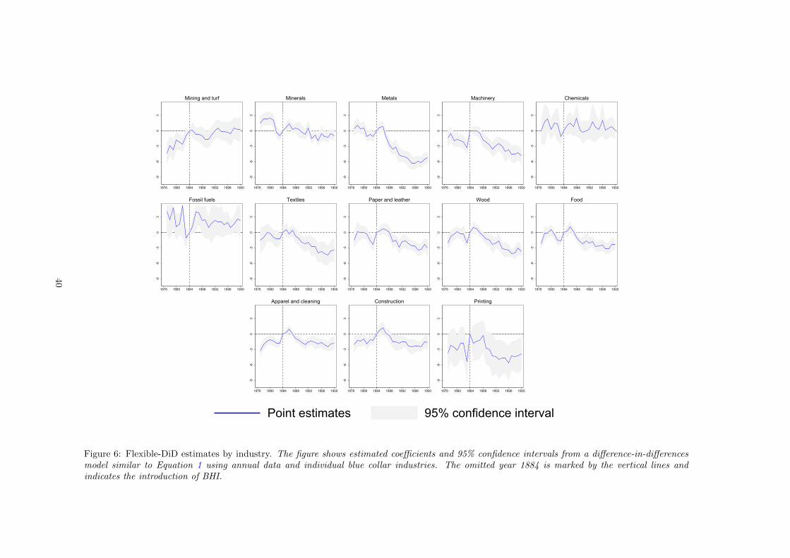
-9-6
-30
3
1876 1880 1884 1888 1892 1896 1900
Mining and turf
-9-6
-30
3
1876 1880 1884 1888 1892 1896 1900
Minerals
-9-6
-30
3
1876 1880 1884 1888 1892 1896 1900
Metals
-9-6
-30
3
1876 1880 1884 1888 1892 1896 1900
Machinery
-9-6
-30
3
1876 1880 1884 1888 1892 1896 1900
Chemicals
-9-6
-30
3
1876 1880 1884 1888 1892 1896 1900
Fossil fuels
-9-6
-30
3
1876 1880 1884 1888 1892 1896 1900
Textiles
-9-6
-30
3
1876 1880 1884 1888 1892 1896 1900
Paper and leather
-9-6
-30
3
1876 1880 1884 1888 1892 1896 1900
Wood
-9-6
-30
3
1876 1880 1884 1888 1892 1896 1900
Food
-9-6
-30
3
1876 1880 1884 1888 1892 1896 1900
Apparel and cleaning
-9-6
-30
3
1876 1880 1884 1888 1892 1896 1900
Construction
-9-6
-30
3
1876 1880 1884 1888 1892 1896 1900
Printing
Point estimates 95% confidence interval
Figure 6: Flexible-DiD estimates by industry. The figure shows estimated coefficients and 95% confidence intervals from a difference-in-differencesmodel similar to Equation 1 using annual data and individual blue collar industries. The omitted year 1884 is marked by the vertical lines andindicates the introduction of BHI.
40
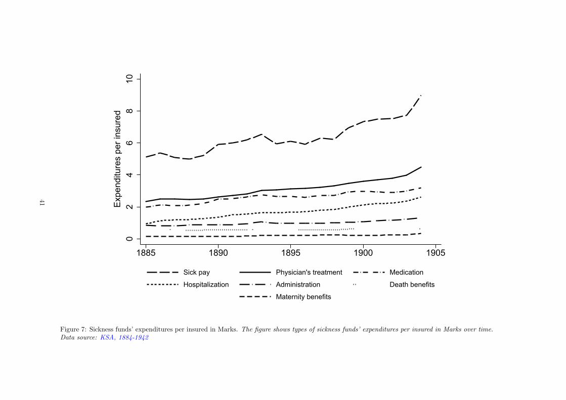
02
46
810
Exp
endi
ture
s pe
r ins
ured
1885 1890 1895 1900 1905
Sick pay Physician's treatment Medication
Hospitalization Administration Death benefits
Maternity benefits
Figure 7: Sickness funds’ expenditures per insured in Marks. The figure shows types of sickness funds’ expenditures per insured in Marks over time.Data source: KSA, 1884-1942
41

Table 1: Sectoral occupation structure
Industrial sector Public sector1882 1895 1907 1882 1895 1907
Total occupational population 9,394 12,196 16,244 1,306 1,672 2,043Working population 3,651 4,756 6,688 587 823 1,027Female working population 585 761 1,078 61 97 166Share in total population 34.4% 38.3% 43.6% 4.8% 5.2% 5.5%Share in working population 31.2% 35.9% 37.1% 5.0% 6.2% 5.7%Share in female working population 17.5% 22.3% 18.7% 1.8% 2.8% 2.9%
Notes: The table reports descriptive statistics based on the occupation censuses conducted in the German Empirein 1882, 1895, and 1907. The industrial sector refers to the official sector B (Industry), while the public sector refersto the official sector E (Public). Absolute population numbers are reported in thousands. The Total OccupationalPopulation includes children and non-employed family members and assigns to them the occupation of the fatheror husband, respectively.
42

Table 2: Flexible DiD: main results
Dep. var.: Deaths per occ. Pop. Baseline Urbanization Waterworks Sewerage(1) (2) (3) (4)
Blue Collar x 1877 -0.1617 -0.3161 -0.3335 -0.2319(0.2272) (0.2410) (0.2146) (0.2255)
Blue Collar x 1885 1.0627*** 1.2011*** 1.1798*** 1.1250***(0.1604) (0.1499) (0.1800) (0.1554)
Blue Collar x 1889 -0.9193*** -0.6621** -0.5766 -0.7835***(0.2761) (0.2563) (0.3603) (0.2811)
Blue Collar x 1893 -1.6119*** -1.2193*** -1.0993** -1.3931***(0.2747) (0.2856) (0.4285) (0.3101)
Blue Collar x 1897 -1.9076*** -1.3332*** -1.2747*** -1.5905***(0.2869) (0.4146) (0.3831) (0.3766)
Urbanization x Sector No Yes No NoWaterworks x Sector No No Yes NoSewerage x Sector No No No YesDistrict x Sector FE Yes Yes Yes YesDistrict x Time FE Yes Yes Yes YesObservations 432 432 432 432R-squared 0.94 0.94 0.94 0.94
Notes: The table reports flexible DiD estimates. All variables are averaged over four year periods from 1877 to 1900. The dependent variable measures crude deaths ratesusing deaths by occupation of the household head per alive occupational population (including dependents) in thousands. The omitted period is 1881-84. Column (2) addsthe urbanization rate as a covariate, column (3) adds waterworks per capita as a covariate, while column (4) adds sewerage per capita as a covariate. Standard errors areclustered at the occupation by district level and given in parentheses. ∗ 10%, ∗∗5%, ∗∗∗ 1% confidence level
43

Table 3: Flexible DiD: heterogeneity
Dep. var.: Deaths per occ. Pop. Baseline Male Female Children(1) (2) (3) (4)
Blue Collar x 1877 -0.1617 0.0573 -0.2390*** 0.0200(0.2272) (0.0695) (0.0584) (0.1585)
Blue Collar x 1885 1.0627*** 0.3741*** 0.0663 0.6223***(0.1604) (0.0701) (0.0425) (0.1126)
Blue Collar x 1889 -0.9193*** -0.4118*** -0.1578*** -0.3497**(0.2761) (0.1079) (0.0536) (0.1738)
Blue Collar x 1893 -1.6119*** -0.5091*** -0.1783*** -0.9244***(0.2747) (0.1011) (0.0548) (0.1774)
Blue Collar x 1897 -1.9076*** -0.5659*** -0.2307*** -1.1110***(0.2869) (0.0927) (0.0669) (0.2112)
District x Sector FE Yes Yes Yes YesDistrict x Time FE Yes Yes Yes YesObservations 432 432 432 432R-squared 0.94 0.92 0.91 0.93
Notes: The table reports flexible DiD estimates. All variables are averaged over four year periods from 1877 to 1900. The dependent variable measures crude deaths ratesusing deaths by occupation of the household head per alive occupational population (including dependents) in thousands. The omitted period is 1881-84. The dependentvariable in column (1) is total mortality, the dependent variable in column (2) is adult male mortality, the dependent variable in column (3) is adult female mortality, and thedependent variable in column (4) is child mortality. Standard errors are clustered at the occupation by district level and given in parentheses. ∗ 10%, ∗∗5%, ∗∗∗ 1% confidencelevel
44

Table 4: County fixed effects using 1882 blue-collar workers’ share
Dep. var.: Crude death rate Base Controls Male Female Infants LegInf IllegInf Placebo(1) (2) (3) (4) (5) (6) (7) (8)
Treatment x 1875 1.891 1.606 -5.714*** 0.711 -20.264* -23.030* 10.630 2.946(1.623) (1.621) (1.713) (1.764) (11.363) (11.948) (56.422) (3.650)
Treatment x 1885 -7.768*** -7.417*** -7.433*** -6.690*** 4.018 1.761 27.650 1.452(1.693) (1.689) (1.965) (1.596) (11.484) (11.989) (47.676) (3.098)
Treatment x 1890 -4.754** -3.983* -6.971*** -6.550*** -19.437 -30.964** 45.986 -1.712(2.041) (2.053) (2.395) (2.079) (15.279) (15.668) (55.537) (3.798)
Treatment x 1895 -8.631*** -7.619*** -5.881** -8.454*** -34.598* -55.767*** 79.660 -3.007(2.080) (2.092) (2.570) (2.153) (20.049) (20.287) (77.044) (4.627)
Treatment x 1900 -12.330*** -11.380*** -16.123*** -13.119*** -45.863* -73.912*** 103.370 1.023(2.399) (2.372) (2.813) (2.500) (24.973) (24.832) (79.473) (4.984)
Controls No Yes Yes Yes Yes Yes Yes YesCounty FE Yes Yes Yes Yes Yes Yes Yes YesTime FE Yes Yes Yes Yes Yes Yes Yes YesObservations 2645 2645 2645 2645 2645 2645 2645 2645Counties 441 441 441 441 441 441 441 441Periods 6 6 6 6 6 6 6 6R-squared 0.75 0.75 0.74 0.74 0.24 0.27 0.03 0.75
Notes: The table reports county-level fixed effects estimates. All variables are averaged over five year periods from 1875 to 1904. The dependent variable measures crude deathrates using total deaths per alive population in thousands. The dependent variable in columns (1), (2), and (8) is total mortality, the dependent variable in column (3) is malemortality, the dependent variable in column (4) is female mortality, and the dependent variable in column (5) is infant mortality (< 1 year) per 1,000 births. The dependentvariable in column (6) is infant mortality (< 1 year) born in wedlock per 1,000 births in wedlock, while the dependent variable in column (7) is infant mortality (< 1 year) bornout of wedlock per 1,000 births out of wedlock. The treatment variable in columns (1) to (7) is the blue collar workers’ population share in 1882, interacted with time-perioddummies. The treatment variable in column (8) is public servants’ population share in 1882, interacted with time-period dummies. The treatment variable in column (8) ispublic servants’ population share in 1882, interacted with time-period dummies. Column (2) adds the urbanization rate, waterworks per capita, and sewerage per capita ascovariates. The omitted period is 1880-84. Standard errors are clustered at the county level and given in parentheses. ∗ 10%, ∗∗5%, ∗∗∗ 1% confidence level
45

Table 5: Robustness tests using district-level data
Initial Blue Collar Workers (1882) Initial Insured (1885)Dep. var.: Crude DR Controls Average age Age groups SPD vote Controls Average age Age groups SPD vote
(1) (2) (3) (4) (5) (6) (7) (8)Treatment x 1875 3.41 3.46 -10.56** 2.88 4.59 4.67 -9.35** 4.48
(4.47) (4.40) (4.57) (4.28) (5.13) (5.12) (4.34) (5.00)Treatment x 1885 -11.14** -11.77** -9.19** -10.91** -15.21** -14.96** -12.45*** -14.85**
(5.30) (5.22) (3.61) (5.33) (6.51) (6.64) (4.44) (6.69)Treatment x 1890 -7.27 -8.49 -8.04 -5.84 -12.53 -11.90 -11.27 -11.11
(8.55) (8.57) (7.34) (8.38) (11.02) (11.13) (8.86) (11.22)Treatment x 1895 -11.97 -12.96* -11.28* -10.40 -17.87** -17.76* -13.52** -16.81*
(7.23) (6.82) (5.83) (7.23) (8.52) (9.08) (6.37) (9.50)Treatment x 1900 -14.91** -16.39** -17.04** -13.19* -22.79*** -22.70*** -21.39*** -21.63**
(6.80) (6.31) (7.10) (6.85) (7.40) (8.17) (7.84) (8.67)Standard controls Yes Yes Yes Yes Yes Yes Yes YesAverage age No Yes No No Yes No No NoAge groups No No Yes No No No Yes NoSPD vote No No No Yes No No No YesDistrict FE Yes Yes Yes Yes Yes Yes Yes YesTime FE Yes Yes Yes Yes Yes Yes Yes YesObservations 216 216 216 216 216 216 216 216Districts 36 36 36 36 36 36 36 36Periods 6 6 6 6 6 6 6 6R-squared 0.88 0.89 0.92 0.88 0.89 0.89 0.92 0.89
Notes: The table reports district-level fixed effects estimates. All variables are averaged over five year periods from 1875 to 1904. The dependent variable is the crude deathrate measured as total deaths per alive population in thousands. The treatment variable in columns (1) to (4) is blue collar workers’ population share in 1882 interacted withtime-period dummies. The treatment variable in columns (5) to (8) is the share of the population covered by health insurance observed in 1885 interacted with time-perioddummies. Standard controls include the urbanization rate, waterworks per capita, and sewerage per capita. In columns (2) and (6), the average age of a district’s population isincluded as a covariate. In columns (3) and (7), we add seven time-varying variables capturing the size of age cohorts as a fraction of the total population (cohorts: 1-9, 10-19,20-29, 30-39, 40-49, 50-59, 60-69, 70 plus). In columns (4) and (8), the vote share of the workers’ party SPD (and its predecessors) measured at the latest general elections isincluded as a covariate. The omitted period is 1880-84. Standard errors are clustered at the district level and given in parentheses. ∗ 10%, ∗∗5%, ∗∗∗ 1% confidence level
46

Table 6: District fixed effects: causes of death
InfectiousDep. var.: Crude DR Accident Waterborne Airborne Lung TB+Scrofula Non-infectious Maternal Unknown
(1) (2) (3) (4) (5) (6) (7) (8)Treatment x 1875 0.162 3.299* -3.962** -3.175* -0.736 -0.571 -0.030 2.087
(0.155) (1.749) (1.707) (1.627) (0.791) (0.873) (0.101) (1.273)Treatment x 1885 -0.090 2.324 -8.606*** -1.493 -0.396 -0.874** -0.186*** -0.305
(0.151) (2.053) (2.721) (1.785) (0.714) (0.371) (0.068) (1.390)Treatment x 1890 0.271* 1.803 -4.561 -3.911 -3.317*** -1.243** -0.186** 1.857
(0.136) (3.221) (4.315) (2.741) (0.931) (0.563) (0.084) (2.023)Treatment x 1895 0.290** 0.422 -4.916 -7.272*** -5.842*** -1.891** -0.183** 3.581
(0.139) (4.169) (3.638) (2.387) (1.215) (0.720) (0.078) (2.212)Treatment x 1900 0.426** 0.602 -8.062*** -11.007*** -8.464*** -3.436*** -0.053 4.412*
(0.169) (3.968) (2.891) (1.982) (1.745) (0.990) (0.114) (2.500)Controls Yes Yes Yes Yes Yes Yes Yes YesDistrict FE Yes Yes Yes Yes Yes Yes Yes YesTime FE Yes Yes Yes Yes Yes Yes Yes YesObservations 216 216 216 216 216 216 216 216Districts 36 36 36 36 36 36 36 36Periods 6 6 6 6 6 6 6 6R-squared 0.54 0.27 0.80 0.60 0.86 0.28 0.92 0.79
Notes: The table reports district-level fixed effects estimates. All variables are averaged over five year periods from 1875 to 1904. The dependent variable measures deathrates by causes of death using total deaths per alive population in thousands. The treatment variable is blue collar workers’ population share observed in 1882 interacted withtime-period dummies. Accident is death from accidents; Waterborne is death from typhus, typhoid fever, and three types of diarrheal diseases; Airborne is death from smallpox,scarlet fever, measles, diphtheria, pertussis, scrofula, tuberculosis, tracheitis, pneumonia and other lung diseases; Lung is death from pertussis, scrofula, tuberculosis, pneumoniaand other lung diseases; TB+Scrofula is death from scrofula and tuberculosis; Non-infectious is death from cancer, edema, stroke, heart disease, brain disease, and kidneydisease; Maternal is maternal death related to childbirth; Unknown is unknown or unspecified cause of death. Controls include the urbanization rate, waterworks per capita,and sewerage per capita. The omitted period is 1880-84. Standard errors, are clustered at the district level and given in parentheses. ∗ 10%, ∗∗5%, ∗∗∗ 1% confidence level.
47

Table 7: Mortality and health expenditures
Panel A - Dependent variable: Crude death rate; Explanatory variable as indicated in column headHealth care expenditures Compensation expenditures Administration Days of
Doctor visits Medication Hospitalization Sickpay Maternity ben. Death ben. expenditures sick leave(1) (2) (3) (4) (5) (6) (7) (8)
L.Expenditure(std) -0.114** -0.160*** -0.042 -0.013 -0.062* 0.065 -0.081 -0.038(0.056) (0.042) (0.072) (0.071) (0.036) (0.040) (0.064) (0.036)
Controls Yes Yes Yes Yes Yes Yes Yes YesDistrict FE Yes Yes Yes Yes Yes Yes Yes YesTime FE Yes Yes Yes Yes Yes Yes Yes YesObservations 684 684 684 684 684 684 684 576Districts 36 36 36 36 36 36 36 36Periods 19 19 19 19 19 19 19 16R-squared 0.81 0.81 0.80 0.80 0.80 0.80 0.80 0.79
Panel B - Dependent variable: Crude death rate by cause of death as indicated in column head; Explanatory variable as indicatedInfectious
All Accident Waterborne Airborne Lung TB+Scrofula Non-infectious Maternal(1) (2) (3) (4) (5) (6) (7) (8)
L.Health care(std) -0.139* 0.079 -0.225 -0.043 -0.302*** -0.333*** -0.196* 0.095(0.070) (0.111) (0.147) (0.107) (0.106) (0.103) (0.100) (0.063)
L.Compensation(std) 0.003 0.059 -0.033 0.047 0.019 0.010 -0.080 -0.062(0.053) (0.116) (0.074) (0.069) (0.103) (0.091) (0.064) (0.057)
L.Administration(std) -0.024 0.092 -0.153 -0.088 -0.182* -0.079 0.075 0.052(0.050) (0.098) (0.137) (0.104) (0.104) (0.098) (0.076) (0.070)
Controls Yes Yes Yes Yes Yes Yes Yes YesDistrict FE Yes Yes Yes Yes Yes Yes Yes YesTime FE Yes Yes Yes Yes Yes Yes Yes YesObservations 612 612 612 612 612 612 612 612Districts 36 36 36 36 36 36 36 36Periods 17 17 17 17 17 17 17 17R-squared 0.75 0.17 0.52 0.69 0.60 0.78 0.26 0.70
Notes: The table reports district-level fixed effects estimates. The dependent variable measures crude death rates using total annual deaths per alive population in thousands(panel A) or annual death rates by cause of death per alive population in thousands (panel B). Accident is death from accidents; Waterborne is death from typhus, typhoidfever, and three types of diarrheal diseases; Airborne is death from smallpox, scarlet fever, measles, diphtheria, pertussis, scrofula, tuberculosis, tracheitis, pneumonia and otherlung diseases; Lung is death from pertussis, scrofula, tuberculosis, pneumonia and other lung diseases; TB+Scrofula is death from scrofula and tuberculosis; Non-infectious isdeath from cancer, edema, stroke, heart disease, brain disease, and kidney disease; Maternal is maternal death related to childbirth. Explanatory variables are sickness funds’expenditures per insured or duration of sick leave per insured lagged by one year. All variables are normalized to a mean zero and a standard deviation of one. Controls includethe urbanization rate, waterworks per capita, and sewerage per capita, each lagged by one year. Standard errors are clustered at the district level and given in parentheses. ∗
10%, ∗∗5%, ∗∗∗ 1% confidence level.
48
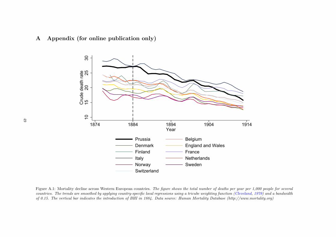
A Appendix (for online publication only)
1015
2025
30C
rude
dea
th ra
te
1874 1884 1894 1904 1914Year
Prussia BelgiumDenmark England and WalesFinland FranceItaly NetherlandsNorway SwedenSwitzerland
Figure A.1: Mortality decline across Western European countries. The figure shows the total number of deaths per year per 1,000 people for severalcountries. The trends are smoothed by applying country-specific local regressions using a tricube weighting function (Cleveland, 1979) and a bandwidthof 0.15. The vertical bar indicates the introduction of BHI in 1884. Data source: Human Mortality Database (http://www.mortality.org)
49

0.2
.4.6
.81
EC
DF
of W
ater
wor
ks
05
1015
2025
Freq
uenc
y
1825 1835 1845 1855 1865 1875 1885 1895Waterworks established p.a.
Frequency ECDF of Waterworks
Figure A.2: The roll-out of waterworks in Prussia. The figure shows the roll-out of waterworks in Prussian cities over time. The bars indicate theannual number of new waterworks put into service. The line indicates the cumulative distribution function. Data source: Grahn (1898-1902)
50

0.2
.4.6
.81
EC
DF
of S
ewag
e
05
1015
20Fr
eque
ncy
1850 1860 1870 1880 1890 1900 1910Sewages established p.a.
Frequency ECDF of Sewage
Figure A.3: The roll-out of sewerage in Prussia. The figure shows the roll-out of sewerage systems in Prussian cities over time. The bars indicatethe annual number of new sewerage put into service. The line indicates the cumulative distribution function. Data source: Salomon (1906-1907)
51

-0.4
-0.3
-0.2
-0.1
0.0
0.1
Coe
ffici
ent e
stim
ate
1876 1880 1884 1888 1892 1896 1900
Point estimates 95% confidence interval
Figure A.4: Flexible-DiD estimates in log-specification. The figure shows estimated coefficients and 95% confidence intervals from a difference-in-differences model similar to Equation 1 using annual data and accounting for pre-trends. The omitted year 1884 is marked by the vertical bar andindicates the introduction of BHI.
52

-4-2
02
4C
oeffi
cien
t est
imat
e
1876 1880 1884 1888 1892 1896 1900
Point estimates 95% confidence interval
Figure A.5: Flexible-DiD estimates using 1890 as reference. The figure shows estimated coefficients and 95% confidence intervals from a difference-in-differences model similar to Equation 1 using annual data and accounting for pre-trends. The omitted year 1890 is marked by the vertical bar andindicates the introduction of the old-age pension system.
53

510
1520
2530
Cru
de d
eath
rate
1876 1880 1884 1888 1892 1896 1900year
Preussen
510
1520
2530
Cru
de d
eath
rate
1876 1880 1884 1888 1892 1896 1900year
Brandenburg
510
1520
2530
Cru
de d
eath
rate
1876 1880 1884 1888 1892 1896 1900year
Pommern
510
1520
2530
Cru
de d
eath
rate
1876 1880 1884 1888 1892 1896 1900year
Posen
510
1520
2530
Cru
de d
eath
rate
1876 1880 1884 1888 1892 1896 1900year
Schlesien
510
1520
2530
Cru
de d
eath
rate
1876 1880 1884 1888 1892 1896 1900year
Sachsen
510
1520
2530
Cru
de d
eath
rate
1876 1880 1884 1888 1892 1896 1900year
Schleswig
510
1520
2530
Cru
de d
eath
rate
1876 1880 1884 1888 1892 1896 1900year
Hannover
510
1520
2530
Cru
de d
eath
rate
1876 1880 1884 1888 1892 1896 1900year
Westfalen
510
1520
2530
Cru
de d
eath
rate
1876 1880 1884 1888 1892 1896 1900year
Hessen-Nassau
510
1520
2530
Cru
de d
eath
rate
1876 1880 1884 1888 1892 1896 1900year
Rheinland
Blue collar workers Public servantsBlue collar workers - counterfactual
Figure A.6: Crude death rates by sector (blue collar workers and public servants) and province. The figure shows the number of deaths per 1,000 peopleby sectoral groups of blue-collar workers and public servants for each Prussian province. Following a difference-in-differences logic, the counterfactualis computed by parallel-shifting the trend of the public servants up to the blue collar workers level in 1884. The vertical bars indicate the introductionof BHI in 1884.
54
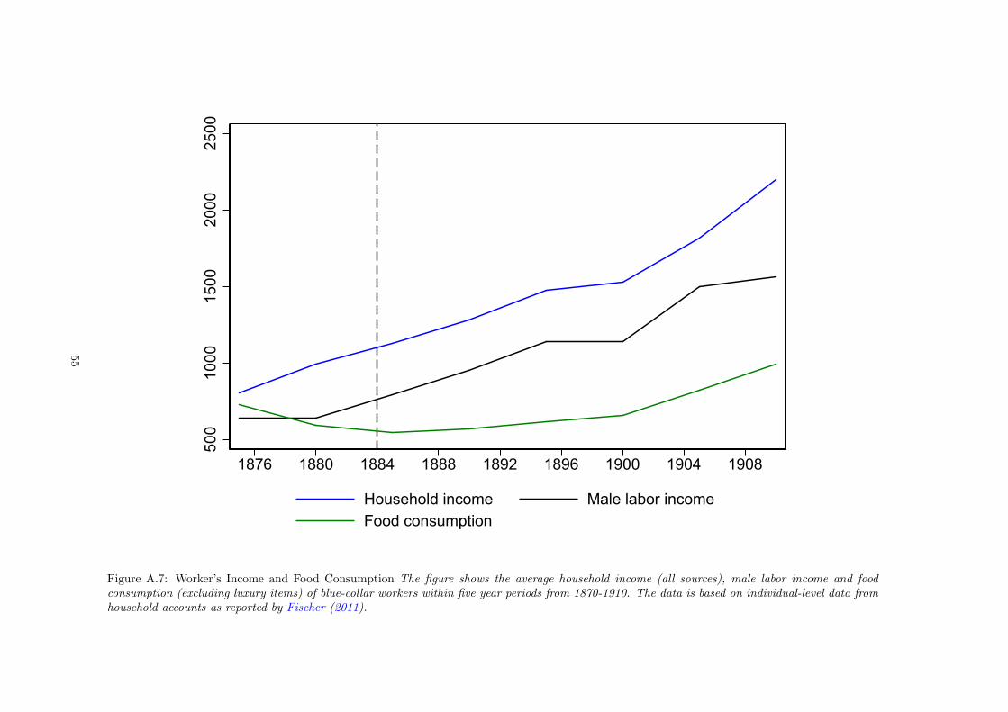
500
1000
1500
2000
2500
1876 1880 1884 1888 1892 1896 1900 1904 1908
Household income Male labor incomeFood consumption
Figure A.7: Worker’s Income and Food Consumption The figure shows the average household income (all sources), male labor income and foodconsumption (excluding luxury items) of blue-collar workers within five year periods from 1870-1910. The data is based on individual-level data fromhousehold accounts as reported by Fischer (2011).
55

Table A1: Expansion of health insurance
Year Population Health Insured % Insured Population1854 17,077 254 1.5%1860 18,136 329 1.8%1864 19,149 458 2.4%1868 24,069 688 2.9%1870 24,403 632 2.6%1872 24,801 725 2.9%1874 25,352 795 3.1%1876 25,922 785 3.0%1885 28,232 2,263 8.0%1890 29,819 3,457 11.6%1895 31,697 3,998 12.6%1900 34,254 5,123 15.0%1905 37,058 6,192 16.7%
Notes: The table shows descriptive statistics on the expansion of health insurance in Prussia within its respectiveborders. Population and the number of insured are expressed in thousands. Insurance benefits vary pre- andpost-1884.
56

Table A2: District fixed effects using blue collar workers and insured population
Initial Blue Collar Workers (1882) Initial Insured (1885)Dep. var.: Crude DR Base Controls Male Female LegInf Base Controls Male Female LegInf
(1) (2) (3) (4) (5) (6) (7) (8) (9) (10)Treatment x 1875 3.37 3.41 -3.19 2.01 13.30 5.04 4.67 -3.48 3.56 17.71
(3.35) (4.47) (4.41) (5.40) (42.84) (4.30) (5.12) (4.70) (6.44) (49.36)Treatment x 1885 -11.19** -11.14** -12.34** -12.20** -23.87 -15.01** -14.96** -15.55** -15.69** -54.41
(4.60) (5.30) (5.72) (5.31) (41.39) (6.11) (6.64) (7.33) (6.75) (47.36)Treatment x 1890 -7.07 -7.27 -12.25 -12.51 -93.97 -11.27 -11.90 -18.87 -18.04 -153.11*
(7.90) (8.55) (11.15) (9.37) (71.55) (10.65) (11.13) (14.44) (12.21) (83.26)Treatment x 1895 -11.64 -11.97 -12.13 -15.64* -154.22 -16.73* -17.76* -19.48 -22.39** -234.92**
(6.98) (7.23) (9.97) (7.82) (93.18) (9.16) (9.08) (12.68) (9.72) (105.54)Treatment x 1900 -15.05** -14.91** -19.21** -19.20** -162.05* -21.83** -22.70*** -28.81** -28.66*** -242.41**
(7.27) (6.80) (9.42) (7.18) (88.70) (9.00) (8.17) (11.68) (8.52) (99.95)Controls No Yes Yes Yes Yes No Yes Yes Yes YesDistrict FE Yes Yes Yes Yes Yes Yes Yes Yes Yes YesTime FE Yes Yes Yes Yes Yes Yes Yes Yes Yes YesObservations 216 216 216 216 216 216 216 216 216 216Districts 36 36 36 36 36 36 36 36 36 36Periods 6 6 6 6 6 6 6 6 6 6R-squared 0.88 0.88 0.85 0.86 0.47 0.88 0.89 0.86 0.87 0.49
Notes: The table reports district-level fixed effects estimates. All variables are averaged over five year periods from 1875 to 1904. The dependent variable in columns (1), (2), (6),and (7) is crude death rates measured as total deaths per alive population in thousands. The dependent variable in columns (3) and (8) is male mortality, the dependent variablein columns (4) and (9) is female mortality, and the dependent variable in columns (5) and (10) is infant mortality (< 1 year) born in wedlock per 1,000 births in wedlock. Thetreatment variable in columns (1)-(5) is blue collar workers’ population share observed in 1882 interacted with time-period dummies. The treatment variable in columns (6)-(10)is the share of the population covered by health insurance in 1885 interacted with time-period dummies. The omitted period is 1880-84. Controls include the urbanization rate,waterworks per capita, and sewerage per capita. Standard errors are clustered at the district level and given in parentheses. ∗ 10%, ∗∗5%, ∗∗∗ 1% confidence level
57

Table A3: The supply of health services
Initial Blue Collar Workers (1882)Dep. var.: Doctors Hospital Patients
(1) (2)Treatment x 1875 -0.19
(0.17)Treatment x 1885 -0.06 0.01**
(0.08) (0.00)Treatment x 1890 0.04 0.03***
(0.09) (0.01)Treatment x 1895 0.34 0.04***
(0.28) (0.01)Treatment x 1900 0.43
(0.40)Controls Yes YesDistrict FE Yes YesTime FE Yes YesObservations 216 144Districts 36 36Periods 6 4R-squared 0.73 0.81
Notes: The table reports district-level fixed effects estimates. The treatment variable is blue collar workers’ population share observed in 1882 interacted with time-perioddummies. The dependent variable in column (1) is the number of licensed doctors per capita. The dependent variable in column (2) is the number of inpatients in hospitals(unavailable prior to 1880). Controls include the urbanization rate, waterworks per capita, and sewerage per capita. The omitted period is 1880-84. Standard errors are clusteredat the district level and given in parentheses. ∗ 10%, ∗∗5%, ∗∗∗ 1% confidence level
58
Top Related