


Languages
Pages
Legal


Air Force Institute of TechnologyAFIT Scholar
Theses and Dissertations Student Graduate Works
3-14-2014
Binary Detection Using Multi-Hypothesis Log-Likelihood, Image ProcessingBrent H. Gessel
Follow this and additional works at: https://scholar.afit.edu/etd
This Thesis is brought to you for free and open access by the Student Graduate Works at AFIT Scholar. It has been accepted for inclusion in Theses andDissertations by an authorized administrator of AFIT Scholar. For more information, please contact [email protected].
Recommended CitationGessel, Brent H., "Binary Detection Using Multi-Hypothesis Log-Likelihood, Image Processing" (2014). Theses and Dissertations. 604.https://scholar.afit.edu/etd/604

BINARY DETECTION USING MULTI-HYPOTHESIS LOG-LIKELIHOOD,
IMAGE PROCESSING
THESIS
Brent H. Gessel, Captain, USAF
AFIT-ENG-14-M-34
DEPARTMENT OF THE AIR FORCEAIR UNIVERSITY
AIR FORCE INSTITUTE OF TECHNOLOGY
Wright-Patterson Air Force Base, Ohio
DISTRIBUTION STATEMENT A:APPROVED FOR PUBLIC RELEASE; DISTRIBUTION UNLIMITED

The views expressed in this thesis are those of the author and do not reflect the officialpolicy or position of the United States Air Force, the Department of Defense, or the UnitedStates Government.
This material is declared a work of the U.S. Government and is not subject to copyrightprotection in the United States.

AFIT-ENG-14-M-34
BINARY DETECTION USING MULTI-HYPOTHESIS LOG-LIKELIHOOD,
IMAGE PROCESSING
THESIS
Presented to the Faculty
Department of Electrical and Computer Engineering
Graduate School of Engineering and Management
Air Force Institute of Technology
Air University
Air Education and Training Command
in Partial Fulfillment of the Requirements for the
Degree of Master of Science in Electrical Engineering
Brent H. Gessel, B.S.E.E.
Captain, USAF
March 2014
DISTRIBUTION STATEMENT A:APPROVED FOR PUBLIC RELEASE; DISTRIBUTION UNLIMITED

AFIT-ENG-14-M-34
BINARY DETECTION USING MULTI-HYPOTHESIS LOG-LIKELIHOOD,
IMAGE PROCESSING
Brent H. Gessel, B.S.E.E.Captain, USAF
Approved:
//signed//
Stephen C. Cain, PhD (Chairman)
//signed//
Keith T. Knox, PhD (Member)
//signed//
Mark E. Oxley, PhD (Member)
20 Feb 2014
Date
13 Feb 2014
Date
20 Feb 2014
Date
AFIT-ENG-14-M-34Abstract
One of the United States Air Force missions is to track space objects. Finding planets,
stars, and other natural and synthetic objects are all impacted by how well the tools of
measurement can distinguish between these objects when they are in close proximity. In
astronomy, the term binary commonly refers to two closely spaced objects. Splitting a
binary occurs when two objects are successfully detected. The physics of light, atmospheric
distortion, and measurement imperfections can make binary detection a challenge.
Binary detection using various post processing techniques can significantly increase
the probability of detection. This paper explores the potential of using a multi-hypothesis
approach. Each hypothesis assumes one two or no points exists in a given image. The log-
likelihood of each hypothesis are compared to obtain detection results. Both simulated and
measured data are used to demonstrate performance with various amounts of atmosphere,
and signal to noise ratios. Initial results show a significant improvement when compared
to a detection via imaging by correlation. More work exists to compare this technique to
other binary detection algorithms and to explore cluster detection.
iv

Table of Contents
Page
Abstract . . . . . . . . . . . . . . . . . . . . . . . . . . . . . . . . . . . . . . . . . iv
Table of Contents . . . . . . . . . . . . . . . . . . . . . . . . . . . . . . . . . . . . v
List of Figures . . . . . . . . . . . . . . . . . . . . . . . . . . . . . . . . . . . . . . vii
List of Tables . . . . . . . . . . . . . . . . . . . . . . . . . . . . . . . . . . . . . . x
List of Acronyms . . . . . . . . . . . . . . . . . . . . . . . . . . . . . . . . . . . . xi
I. Introduction . . . . . . . . . . . . . . . . . . . . . . . . . . . . . . . . . . . . . 1
1.1 Binary detection . . . . . . . . . . . . . . . . . . . . . . . . . . . . . . . . 11.2 Space situational awareness . . . . . . . . . . . . . . . . . . . . . . . . . . 21.3 Research objectives . . . . . . . . . . . . . . . . . . . . . . . . . . . . . . 31.4 Organization . . . . . . . . . . . . . . . . . . . . . . . . . . . . . . . . . . 3
II. Background . . . . . . . . . . . . . . . . . . . . . . . . . . . . . . . . . . . . . 5
2.1 Post-Process Imaging . . . . . . . . . . . . . . . . . . . . . . . . . . . . . 82.1.1 Atmospheric Turbulence . . . . . . . . . . . . . . . . . . . . . . . 82.1.2 Deconvolution . . . . . . . . . . . . . . . . . . . . . . . . . . . . 11
2.1.2.1 Knox-Thompson . . . . . . . . . . . . . . . . . . . . . . 162.1.2.2 Bispectrum . . . . . . . . . . . . . . . . . . . . . . . . . 19
2.1.3 Imaging by Correlation . . . . . . . . . . . . . . . . . . . . . . . . 222.1.4 Binary detection by post-process image reconstruction summary . . 26
2.2 Multi-Hypothesis Detection . . . . . . . . . . . . . . . . . . . . . . . . . . 262.3 Chapter Summary . . . . . . . . . . . . . . . . . . . . . . . . . . . . . . . 28
III. Methodology . . . . . . . . . . . . . . . . . . . . . . . . . . . . . . . . . . . . 29
3.1 Derivation of multi-hypothesis algorithms . . . . . . . . . . . . . . . . . . 303.1.1 Zero point source derivation . . . . . . . . . . . . . . . . . . . . . 303.1.2 Single point source derivation . . . . . . . . . . . . . . . . . . . . 313.1.3 Two point source derivation . . . . . . . . . . . . . . . . . . . . . 34
3.2 Software implementation . . . . . . . . . . . . . . . . . . . . . . . . . . . 383.2.1 Point source threshold . . . . . . . . . . . . . . . . . . . . . . . . 383.2.2 zero point source implementation . . . . . . . . . . . . . . . . . . 39
v

Page
3.2.3 Single point source implementation . . . . . . . . . . . . . . . . . 393.2.4 Two point source implementation . . . . . . . . . . . . . . . . . . 403.2.5 Decision process . . . . . . . . . . . . . . . . . . . . . . . . . . . 41
3.3 Simulation test model . . . . . . . . . . . . . . . . . . . . . . . . . . . . . 433.3.1 Modeling atmospheric effects . . . . . . . . . . . . . . . . . . . . 433.3.2 Test variables . . . . . . . . . . . . . . . . . . . . . . . . . . . . . 443.3.3 Performance measurements for simulated data . . . . . . . . . . . 453.3.4 Simulated comparison model . . . . . . . . . . . . . . . . . . . . . 45
3.4 Measured data test model . . . . . . . . . . . . . . . . . . . . . . . . . . . 463.4.1 Description of measured data . . . . . . . . . . . . . . . . . . . . . 463.4.2 Deriving a valid PSF . . . . . . . . . . . . . . . . . . . . . . . . . 473.4.3 Determining success of measured data test . . . . . . . . . . . . . 47
IV. Results . . . . . . . . . . . . . . . . . . . . . . . . . . . . . . . . . . . . . . . . 48
4.1 Multi-hypothesis binary detection simulation results . . . . . . . . . . . . . 484.1.1 Image generation . . . . . . . . . . . . . . . . . . . . . . . . . . . 504.1.2 Log-likelihood bias correction . . . . . . . . . . . . . . . . . . . . 534.1.3 Probability of Detection (PD) sample results . . . . . . . . . . . . . 534.1.4 Probability of false alarm (P f a) simulation results . . . . . . . . . . 564.1.5 PD and P f a result summary . . . . . . . . . . . . . . . . . . . . . . 58
4.2 Comparison with imaging by correlation technique . . . . . . . . . . . . . 584.2.1 Probability of False Alarm (P f a) comparison results . . . . . . . . 604.2.2 Probability of Detection (PD) comparison results . . . . . . . . . . 624.2.3 Comparison result summary . . . . . . . . . . . . . . . . . . . . . 64
4.3 Measured data processing results . . . . . . . . . . . . . . . . . . . . . . . 644.3.1 First image: two points spaced far away . . . . . . . . . . . . . . . 644.3.2 Second image: two points in close proximity . . . . . . . . . . . . 664.3.3 Third image: two points touching . . . . . . . . . . . . . . . . . . 684.3.4 Fourth image: single point . . . . . . . . . . . . . . . . . . . . . . 704.3.5 Measured data result summary . . . . . . . . . . . . . . . . . . . . 72
V. Future work . . . . . . . . . . . . . . . . . . . . . . . . . . . . . . . . . . . . . 73
5.1 Summary . . . . . . . . . . . . . . . . . . . . . . . . . . . . . . . . . . . 735.2 Future work . . . . . . . . . . . . . . . . . . . . . . . . . . . . . . . . . . 73
Bibliography . . . . . . . . . . . . . . . . . . . . . . . . . . . . . . . . . . . . . . 75
vi

List of Figures
Figure Page
2.1 Basic adaptive optic process. . . . . . . . . . . . . . . . . . . . . . . . . . . . 7
2.2 Speckle interferometry simulation with 200 independent frames. (a) The
binary source image, (b) the simulated average of short exposure images, (c)
speckle transfer function, (d) speckle transfer function showing fringe spacing. 14
2.3 Stack of 50 short exposure images, each simulated through a unique random
phase screen with ro = 30 cm. . . . . . . . . . . . . . . . . . . . . . . . . . . 19
2.4 Result of cross spectrum method with ro = 30cm, original image (a),
cross section of original image (b), reconstructed image (c), cross section of
reconstructed image (d). . . . . . . . . . . . . . . . . . . . . . . . . . . . . . 20
2.5 Results with different numbers of iterations: (a) 1, (b) 5, (c) 10, (d) 15, (e) 80,
and (f) 100 iterations. . . . . . . . . . . . . . . . . . . . . . . . . . . . . . . . 24
2.6 Results of the correlation technique: (a) original image, (b) original image
cross section, (c) reconstructed image, and (d) reconstructed image cross section. 25
2.7 Overview of binary hypothesis method. Chapter 3 will work through
derivations of each step. . . . . . . . . . . . . . . . . . . . . . . . . . . . . . . 27
4.1 Sample simulated detected images of binary source with 500 photons for each
point. Samples taken for various background noise and D/r0 values as given
next to each image. Zoomed in to 31x31 pixels. . . . . . . . . . . . . . . . . . 51
4.2 Sample simulated detected images of single point sources used in calculating
false alarm rates. Samples taken for various background noise and D/r0 values
as given next to each image. Zoomed in to a 31x31 pixel area. . . . . . . . . . 52
vii
Figure Page
4.3 False Alarm rate versus D/r0 for a point source with an intensity of 1000
photons for, (a) background noise level=1, (b) background noise level=2, (c)
background noise level=3. . . . . . . . . . . . . . . . . . . . . . . . . . . . . 60
4.4 False Alarm rate versus D/r0 for a point source with an intensity of 1500
photons for, (a) background noise level=1, (b) background noise level=2, (c)
background noise level=3. . . . . . . . . . . . . . . . . . . . . . . . . . . . . 61
4.5 False Alarm rate versus D/r0 for a point source with an intensity of 2000
photons for, (a) background noise level=1, (b) background noise level=2, (c)
background noise level=3. . . . . . . . . . . . . . . . . . . . . . . . . . . . . 61
4.6 Detection rate versus D/r0 for a binary source with an intensities of 500 and
500 photons for, (a) background noise level=1, (b) background noise level=2,
(c) background noise level=3. . . . . . . . . . . . . . . . . . . . . . . . . . . 62
4.7 Detection rate versus D/r0 for a binary source with an intensities of 1000 and
500 photons for, (a) background noise level=1, (b) background noise level=2,
(c) background noise level=3. . . . . . . . . . . . . . . . . . . . . . . . . . . 63
4.8 Detection rate versus D/r0 for a binary source with an intensities of 1000 and
1000 photons for, (a) background noise level=1, (b) background noise level=2,
(c) background noise level=3. . . . . . . . . . . . . . . . . . . . . . . . . . . 63
4.9 First measured image (a) Detected image, (b) Result of hypothesis one, (c)
Result of hypothesis two. The log-likelihood of hypothesis two was larger and
therefore a binary was detected. . . . . . . . . . . . . . . . . . . . . . . . . . 65
4.10 First measured image (a) Detected image, (b) Result of hypothesis one, (c)
Result of hypothesis two. The log-likelihood of hypothesis two was larger and
therefore a binary was detected. . . . . . . . . . . . . . . . . . . . . . . . . . 67
viii

Figure Page
4.11 Third measured image (a) Detected image, (b) Result of hypothesis one, (c)
Result of hypothesis two. The log-likelihood of hypothesis two was larger and
therefore a binary was detected. . . . . . . . . . . . . . . . . . . . . . . . . . 69
4.12 Forth measured image (a) Detected image, (b) Result of hypothesis one, (c)
Result of hypothesis two. The log-likelihood of hypothesis one was greater
and so a binary was not detected. . . . . . . . . . . . . . . . . . . . . . . . . . 71
ix

List of Tables
Table Page
2.1 First 10 Zernike Circular Polynomials [33]. . . . . . . . . . . . . . . . . . . . 10
3.1 Common symbols. . . . . . . . . . . . . . . . . . . . . . . . . . . . . . . . . 29
4.1 Probability of Detection (PD) results using binary source with 500/500 photons. 54
4.2 Probability of Detection (PD) results using binary source with 1000/500 photons. 55
4.3 Probability of Detection (PD) results using binary source with 1000/1000
photons. . . . . . . . . . . . . . . . . . . . . . . . . . . . . . . . . . . . . . . 55
4.4 Probability of False Alarm (P f a) results using point source with 1000 photons. . 56
4.5 Probability of False Alarm (P f a) results using point source with 1500 photons. . 57
4.6 Probability of False Alarm (P f a) results using point source with 2000 photons. . 57
x

List of Acronyms
Acronym Definition
CCD Charge-Coupled Device
PD Probability of Detection
P f a Probability of False Alarm
PSF Point Spread Function
OTF Optical Transfer Function
FT Fourier Transform
PSD Power Spectral Density
LiDAR Light Detection And Ranging
PMF Probability Mass Function
SST Space Surveillance Telescope
DARPA Defense Advanced Research Projects Agency
GEO Geostationary Earth Orbit
xi

BINARY DETECTION USING MULTI-HYPOTHESIS LOG-LIKELIHOOD,
IMAGE PROCESSING
I. Introduction
Comparing statistical hypotheses to determine the likelihood of a given event is a
proven technique used in many fields, particularly digital communication. The
application of a multi-hypothesis test algorithm to the detection of binary stars or other
space objects is an area of new exploration. This thesis will explore the usefulness of using
a multi-hypothesis technique to resolve close binary objects in space. The first task is
to derive a multi-hypothesis algorithm specifically for binary detection and then provide
results for various simulated imaging conditions as well as measured binary images.
Simulated results will be compared with another technique to explore potential detection
improvements.
1.1 Binary detection
The ability to discriminate between closely-spaced objects in space has and continues
to be a challenge. Finding planets, stars, and other natural celestial objects, as well as
trying to keep track of satellites and space debris are all impacted by how well the tools of
measurement can distinguish between these objects in close proximity. In astronomy, the
term binary commonly refers to two stars in the same system. Splitting a binary occurs
when two stars are successfully identified. Some binaries are easily split using basic
equipment. As the source intensity, object distance, and/or atmospheric distortion varies,
the binaries will appear as just a single object. In this paper, the term binary refers to any
two closely spaced objects. Several image post processing techniques have been developed
1

to increase spatial resolution and/or look for patterns common to binary objects. Most of
the commonly used methods today focus on image reconstruction and deblurring. This
thesis will show that if an image’s Point Spread Function (PSF) is known and the source is
a single or double point source, the log-likelihood of the most probable hypothesis provides
a statistical comparison of how likely a blurred image contains a binary.
1.2 Space situational awareness
One of the United States Air Force missions is to track space objects, particularly
of the synthetic kind. Due to the physics of spatial resolution, it is extremely difficult to
resolve satellites in geosynchronous orbit (35,786 km). At this distance the size of a satellite
is typically smaller than one pixel on a high quality Charge-Coupled Device (CCD) camera.
For example, if a satellite in geosynchronous orbit is 15 meters wide (the length of a full
size school bus) and a telescope with an aperture of 4 meters and focal length of 64 meters
is focused on it, the size on the CCD would be:
size =(sat.size)( f ocal.length)
distance=
(15m)(64m)35, 786, 000m
= 2.64µm. (1.1)
This is much smaller than a typical CCD pixel used in astronomical telescopes. This is also
smaller than the Raleigh criteria for spatial resolution for this same setup [14]:
Resolution ≈ (1.22)(λ)( f /#) = (1.22)(550nm)(16) = 8.48µm (1.2)
where λ is the wavelength of light and f /# is the f-number, which is the focal length divided
by the diameter of the optical system. The atmosphere will further blur this image and after
a certain amount of exposure time the image will typically be a few to several pixels of
light. At this distance, it can be extremely difficult to tell if there is one, two or several
objects in the spot of light.
The multi-hypothesis method discussed in this thesis has the potential to increase
the probability of correctly detecting binaries at geosynchronous orbit and other scenarios
important to the USAF.
2

1.3 Research objectives
The question posed in this thesis is how well, if at all, can a multi-hypothesis model
correctly detect a binary pair in a blurred image? To answer that question four research
objectives are documented.
First, a statistical model is derived in Section 3.1. Here the derivation of algorithms
for zero, one, and two point sources are shown.
The second objective is to successfully implement the mathematical algorithms into
a software simulation model. This model includes atmospheric effects, background
noise, and creates a test environment to work out threshold parameters that maximize the
probability of detection while minimizing the false alarm rate. The simulation will be done
in Matlab™and is covered in Section 3.2.
Once the binary hypothesis method is successfully implemented and results measured,
it is important to compare them to another modern technique. The third objective is to
compare results from another image detection method, specifically imaging by correlation
with a threshold set for binary detection. Section 3.3 walks through an implementation of
imaging by correlation in Matlab™and results are provided in Chapter 4.
The final objective is to use measured imagery data where the number of objects is
known and see how well the algorithm correctly detects when a binary is present. The
imagery data used is focused on a satellite in geosynchronous orbit with a dim star passing
by at various distances, including the situation where the two appear as a single object.
The decision to select a binary from the algorithm is compared against the truth data and
presented in Chapter 4.
1.4 Organization
This research document is organized in accordance with AFIT’s thesis guidelines.
Chapter 2 will discuss current methods used to detect binaries and contrast them with the
proposed, unpublished, multi-hypothesis binary detection method. Chapter 3 provides the
3

derivation and simulation methods used to meet the thesis objectives outlined in the pre-
vious section. Chapter 4 contains the results of several of the simulation tests as well as
the results of processing measured data. Chapter 5 discusses conclusions and opportunities
for continued research and operational testing. Complete references of all sources cited are
contained in the bibliography. Every attempt has been made to use consistent variables to
enhance readability.
4

II. Background
High spatial resolution of an imaging system is key to achieving detection of binary
objects. A standard telescope system cannot achieve diffraction-limited resolution
due to factors such as atmospheric and optical aberration. Several techniques have been
developed to close the gap between diffraction-limited resolution and a system’s actual
resolution. This chapter will discuss some of the most common post-processing techniques
to increase spatial resolution in astronomical imaging. Additionally, a brief overview of
multi-hypothesis statistics is provided.
Binary objects do not all behave in the same way. Although the imaging techniques
discussed in this chapter can be used on all binaries, specific methods have been developed
to look for planets and binary star systems. As gravitational fields of large planets and stars
interact, a periodic movement, often referred to as wobble, can be detected [23]. Other
indicators such as periodic eclipsing and Doppler-like wavelength patterns can infer the
presence of a binary [6]. These methods have been successful on a subset of binaries
but cannot be applied to binaries in general. This paper will not focus on gravitational,
orbital or other spectroscopic measurements techniques, rather the focus will be on post-
processing techniques useful in detecting any binary.
Aside from the natural effect of diffraction, the earth’s atmosphere plays a large
role in limiting spatial resolution. Virtually all real-time and post-processing de-blurring
techniques require an understanding of how the atmosphere is changing the light. Because
we know what a diffraction-limited point source looks like, we can compare it to a
measured point source through the same atmosphere and use that information to correct
the atmospheric distortion [14][12]. Lightwaves from distant point source(s) can be
estimated as plane waves right before reaching earth’s atmosphere [14]. The atmosphere
will randomly distort this wave and the distortion can be measured by a wavefront sensor
5

[33]. Unfortunately, it is impossible to have a perfect natural point source everywhere
in the night sky at visible wavelengths [11][37][38][39]. To overcome this limitation,
one or more lasers can be used to create point sources, or guide beacons, in the area
of interest [7][9][10][11][15][37]. A wavefront sensor takes the point source, or guide
star, information and determines corrective adjustments then sends that data to an adaptive
optics system [32]. Real world performance of adaptive optics can vary from near
diffraction limited correction to no visible improvement depending on a host of factors
[1][8][16][17][28][36][40].
The need for a valid point source cannot be understated since it is foundational to
adaptive optics and the post-processing techniques described in this chapter. A great deal
of research still remains in the field of generating and measuring quality point sources.
Although adaptive optics is an important technique in moving closer to diffraction limited
imaging, it is not currently a practical solution for all imaging sites. Having one or more
image post-processing software solutions is a relatively affordable way to augment or
supplement adaptive optic systems. It is the area of software post-processing that this
paper will focus from this point on.
The following sections will discuss two of the most common post-processing methods
for binary detection, deconvolution and speckle interferometry. Section 2.2 finishes the
chapter with a brief and general look at how multi-hypothesis statistics can be used in
binary detection.
6

RANDOM ATMOSPHERIC TURBULENCE
LIGHTWAVES
POINT SOURCE
TELESCOPE
BEAM SPLITTER
CCD
ADAPTIVE MIRROR
MIRROR CONTROL
WAVEFRONTSENSOR
Figure 2.1: Basic adaptive optic process.
7

2.1 Post-Process Imaging
Image post-processing can be an effective and affordable way to increase image
resolution. This section will look at two deconvolution methods and a speckle
interferometry technique useful for visual binary detection. These processes attempt to
reconstruct a higher resolution image from measured data. It is important to note that the
multi-hypothesis method does not produce a reconstructed image so it is a fundamentally
different approach but still fits within the post-processing category of binary detection.
2.1.1 Atmospheric Turbulence.
Before discussing specific imaging techniques it is important to explain how
atmospheric turbulence is modeled in this thesis. The most common methods utilize
the approximation that atmospheric effects can be represented as wavefront errors in the
pupil plane. If A(u, v) represents the two-dimensional, clear pupil and W(u, v) represents
wavefront error as a function of position with respect to a fixed Cartesian coordinate system,
(u, v), then the atmospherically blurred image, i(x, y), can be represented as:
i(x, y) =∣∣∣∣F {
A(u, v)e jW(u,v)}∣∣∣∣2 (2.1)
where F is the symbol denoting the Fourier Transform. The wavefront error as a function
of position, commonly called a phase screen, can be simulated in various ways. One of the
most common methods of phase screen generation utilizes Power Spectral Density (PSD)
models, such as von Karman and modified von Karman [31]. These are referred to as
Fourier Transform (FT) based methods [31]. The model used in the simulations of this
paper are based upon another method that uses Zernike polynomials to generate phase
screens.
It has been shown that the wavefront error, W(u, v), can be expanded with basis
functions based on the geometry of the aperture [33]. Common basis functions include,
Zernike circular, Zernike annular, Gaussian-circular, and Gaussian-annular. A Zernike
circular set of basis functions were used in this paper to match the geometry of the
8
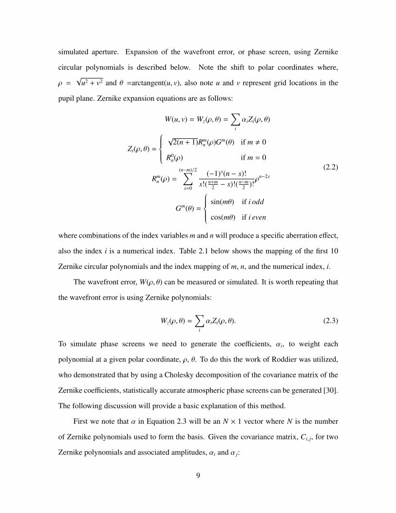
simulated aperture. Expansion of the wavefront error, or phase screen, using Zernike
circular polynomials is described below. Note the shift to polar coordinates where,
ρ =√
u2 + v2 and θ =arctangent(u, v), also note u and v represent grid locations in the
pupil plane. Zernike expansion equations are as follows:
W(u, v) = Wz(ρ, θ) =∑
i
αiZi(ρ, θ)
Zi(ρ, θ) =
√
2(n + 1)Rmn (ρ)Gm(θ) if m , 0
R0n(ρ) if m = 0
Rmn (ρ) =
(n−m)/2∑s=0
(−1)s(n − s)!s!( n+m
2 − s)!( n−m2 )!
ρn−2s
Gm(θ) =
sin(mθ) if i odd
cos(mθ) if i even
(2.2)
where combinations of the index variables m and n will produce a specific aberration effect,
also the index i is a numerical index. Table 2.1 below shows the mapping of the first 10
Zernike circular polynomials and the index mapping of m, n, and the numerical index, i.
The wavefront error, W(ρ, θ) can be measured or simulated. It is worth repeating that
the wavefront error is using Zernike polynomials:
Wz(ρ, θ) =∑
i
αiZi(ρ, θ). (2.3)
To simulate phase screens we need to generate the coefficients, αi, to weight each
polynomial at a given polar coordinate, ρ, θ. To do this the work of Roddier was utilized,
who demonstrated that by using a Cholesky decomposition of the covariance matrix of the
Zernike coefficients, statistically accurate atmospheric phase screens can be generated [30].
The following discussion will provide a basic explanation of this method.
First we note that α in Equation 2.3 will be an N × 1 vector where N is the number
of Zernike polynomials used to form the basis. Given the covariance matrix, Ci, j, for two
Zernike polynomials and associated amplitudes, αi and α j:
9

Table 2.1: First 10 Zernike Circular Polynomials [33].
i m n Zmn (ρ, θ) Name
1 0 0 1 piston
2 1 1 2ρ cos(θ) x tilt
3 1 1 2ρ sin(θ) y tilt
4 0 2√
3(2ρ2 − 1) defocus
5 2 2√
6ρ2 sin(2θ) y primary astigmatism
6 2 2√
6ρ2 cos(2θ) x primary astigmatism
7 1 3√
8(3ρ3 − 2ρ) sin(θ) y primary coma
8 1 3√
8(3ρ3 − 2ρ) cos(θ) x primary coma
9 3 3√
8ρ3 sin(3θ) y primary trefoil
10 3 3√
8ρ3 cos(3θ) x primary trefoil
11 0 4√
5(6ρ4 − 6ρ2 + 1) x primary spherical
Ci, j = E[αi,α j] (2.4)
C = LLT (2.5)
where LT denotes the conjugate transpose of the lower triangular matrix L. The covariance
matrix generated from two Zernike polynomials Zi and Z j has been derived by Knoll
[27][30]:
Ci, j = E[αi, α j] =KZiZ jδZΓ[(ni + n j − 5/3)/2](D/r0)5/3
Γ[(ni − n j − 17/3)/2]Γ[(ni − n j − 17/3)2]Γ[(ni − n j − 23/3)/2](2.6)
where:
KZiZ j =Γ(14/3)[(24/5)Γ(6/5)]5/6[Γ(11/6)]2
2π2 × (−1)(ni+n j−2mi)/2√
(ni + 1)(n j + 1) (2.7)
and:
δZ = [(mi = m j)]∧
[parity(i, j) ∨ (mi = 0)]. (2.8)
10

If we generate a vector of zero mean with unit variance uncorrelated numbers, n, then
we can solve for the amplitudes, α, that weight each Zernike polynomial by applying the
properties of the Cholesky decomposition such that:
L = C12 (2.9)
and:
α = Ln. (2.10)
Thus, given a randomly generated zero mean, unit variance vector n, the Freid seeing
parameter, r0, the diameter of the aperture, D, and the number of Zernike polynomials
desired, a wavefront error phase screen can be calculated. Again, this is the method used in
all simulation conducted as part of this thesis. For more information on this method please
refer to [30].
2.1.2 Deconvolution.
Deconvolution is a de-blurring technique widely used in many fields including
astrophotography. Basically, if an image is distorted with spatially invariant blur, e.g.
the same atmospheric distortion is applied to the entire image, it can be modeled as the
convolution of the measured point spread function and the true image [19]. Or, using the
Convolution Theorem, the Fourier Transform of the image is equal to the Fourier Transform
of the object multiplied by the Optical Transfer Function (OTF):
i(x) = o(x) ⊗ h(x)
F {i(x)} = F {o(x)} × F {h(x)}.(2.11)
In this equation, ⊗ is the convolution operation. Typically, the only information known
is the blurred image and an imperfect point spread function–this is known as blind
deconvolution [19]. By using multiple frames with their respective measured point spread
functions the number of solutions to the blind deconvolution can be reduced [35]. This
is known as multiframe blind deconvolution and is an important technique used for image
11

restoration [5][35].
In 1970, Antoine Labeyrie observed that the speckles in a short exposure image
contained more spatial frequency data when compared to a long exposure image [20].
The processes that use this speckle information to reconstruct an image is referred to as
speckle imaging. There are two main steps to speckle imaging. First, to estimate the object
and reference star intensity and second, to recover the phase that is lost from the first step
[3]. Step one will be described in this section and two methods of phase recovery will be
covered in the next two subsections.
Speckle interferometry is a technique used to find the expected value of the modulus
of the Fourier Transform of the object. If the source object happens to be two points the
cosine fringe patterns can be seen (see Figure 2.2).
If αs represents the angular separation of a binary pair and, λD ≤ αs ≤
λr0
, where λD
is the approximate smallest angular separation two points are detectable in a diffraction
limited environment and λr0
is the smallest approximate angular separation two points can
be detected through atmospheric turbulence then speckle interferometry can be useful [31],
where r0 is the Fried’s seeing parameter and λ is the wavelength of light. If αs <λD , then
the angular separation is too small to resolve. If αs >λr0
, then speckle interferometry will
not improve the resolution. It is therefore assumed going forward that the binary separation
angle, αs, falls within the range above, where deconvolution is helpful.
First consider the irradiance incident on a detector. If the imaging system is properly
focused on the object, we have the incident irradiance equal to the object irradiance as
observed from geometry alone convolved with the PSF:
d(x) =∑
y
h(x − y)o(y) (2.12)
where d(x) is a single measured short exposure image, h(y) is the PSF, and o(y) is
the diffraction-limited object irradiance. If the source object is a binary, let o(y) =
12

o1δ(y) + o2δ(y − y1), where δ is the Dirac function and o1 and o2 are the intensities of
the binary points. Taking the convolution and applying the sifting property of integrating a
Dirac function yields:
d(x) =∑
y
o1h(x − y)δ(y) +∑
y
o2h(x − y)δ(y − y1)
= o1h(x) + o2h(x − y1).
(2.13)
Now take the Fourier transform of d(x):
F {d(x)} = o1H(f) + o2H(f)e− j2πy1 fx . (2.14)
Here we take the modulus squared of the result:
|F {d(x)}|2 =(O1H(f) + O2H(f)e− j2πy1 fx
)×
(O1H(f)∗ + O2H(f)∗e j2πy1 fx
)= O2
1|H(f)|2 + O22|H(f)|2 + 2 × REAL
{O1O2|H(f)|2e− j2πy1 fx
} (2.15)
noting that REAL{e− j2πy1 fx
}= cos (2πy1 fx) reducing Equation 2.15 to:
|F {d(x)}|2 = O21|H(f)|2 + O2
2|H(f)|2 + 2O1O2|H(f)|2 cos(2πy1 fx) (2.16)
divide both sides by |H(f)|2, yields:
|F {d(x)}|2
|H(f)|2= O2
1 + O22 + 2O1O2 cos(2πy1 fx). (2.17)
Let Q(f) = |F {d(x)}|2 − K, where K is the photon noise bias governed by Poisson statistics
and Q(f) is the unbiased speckle interferometry estimator [13]. The signal-to-noise ratio,
S NRQ, of Q(f) improves as follows:
S NRNQ(f) =
√N × S NRQ(f) (2.18)
where S NRNQ is the signal-to-noise ratio of N averaged independent realizations of Q(f)
[31]. Values of N, the number of short exposure images, range from a few hundred to
13

several thousand [31]. Assuming N > 1, it is necessary to take the expected value of both
the numerator and denominator of Equation 2.17:
E{|F {i(x)}|2}E{|H(f)|2}
= O21 + O2
2 + 2O1O2 cos(2πy1 fx) (2.19)
where i(x) is the detection plane irradiance of N images, H(f) is the OTF and y1 is the
separation of the binary stars, O1(f) and O2(f) is the image spectrum of the binary stars.
Plotting the results of Equation 2.19 can reveal a cosine pattern if the angular separation of
the binary pair is large enough [14][20][31].
The following is a simulated example of speckle interferometry using 200 independent
images of two point sources.
(a)
P1:124,128 → ← P2:132,128
110 120 130 140 150
105
110
115
120
125
130
135
140
145
150
(b)
50 100 150 200 250
50
100
150
200
250
(c)
50 100 150 200 250
50
100
150
200
250
(d)
113,128 → ← 145,128
50 100 150 200 250
50
100
150
200
250
Figure 2.2: Speckle interferometry simulation with 200 independent frames. (a) The binary
source image, (b) the simulated average of short exposure images, (c) speckle transfer
function, (d) speckle transfer function showing fringe spacing.
In Figure 2.2 (a) the binary source image is shown, note the separation is 8 pixels; (b) is
the simulated average of 200 short exposure images; (c) is the calculated unbiased speckle
14

interferometry estimator, Q(f) (log scale); finally, (d) shows the log scale of Q(f)E{|H(f)|2} . The
binary separation from the original image, y1 can be calculated from the results. First
looking at Equation 2.19, the period of the fringe pattern detected depends on cos(2πy1 fx).
Where y1 is a 2-tuple and denotes the location of the second binary point in the image plane
and fx is the size of a pixel in the frequency plane. The peak-to-peak period in pixel count
of the cosine fringes in Figure 2.2 (d) is 32:
P = Period =1
f requency=
1y1∆ fx
∆ fx =1N
(2.20)
where N = 256, the number of pixels and ∆ fx is the sample size in the frequency plane.
P = Period =256y1
from measurements, P=32 pixels :
32 =256y1
y1 =25632
= 8 pixels.
(2.21)
Looking at the simulation parameters, 8 pixels was the binary separation used to generate
the image. The actual physical interpretation of 8 pixels of separation will depend on the
characteristics of the imaging system and distance to the object being viewed. Thus, by
measuring the pixel separation of the binary fringe pattern an estimation can be made as to
the actual binary separation in the object plane.
Observing these cosine fringe patterns is a proven method of finding binary point
sources. However, as mentioned before, the phase data is lost after taking the second
moment of the image spectrum. This phase data needs to be recovered for image
reconstruction. The next two subsections will discuss two common methods of phase
retrieval.
15

2.1.2.1 Knox-Thompson.
As stated before, to properly reconstruct an image using spectral imaging the phase of
the source object needs to be recovered. The first technique commonly used is the Knox-
Thompson or cross spectrum method. Dr. K. T. Knox and B. J. Thompson published a
paper in the Astrophysics Journal in 1974 describing a method of recovering images from
atmospherically-degraded short exposure images [18][31]. This method is now called the
Knox-Thompson Technique or the cross spectrum technique. In their paper, they defined
the cross spectrum, C(f,∆f), as:
C(f,∆f) = I(f)I∗(f + ∆f) (2.22)
where I(f) = O(f)H(f) and O(f) is the object spectrum, and H(f) is the OTF [31][18].
The cross spectrum of the detected image is not directly proportional to the cross
spectrum of the object as a bias term needs to be accounted for to properly estimate the
phase [2][4][31]. If we assume individual pixels in the detection plane are statistically in-
dependent and the photon arrival is governed by Poisson statistics, then the unbiased cross
spectrum for a single measured image, d(x), can be written as [31]:
Cu(f,∆f) = D(f)D∗(f + ∆f) − D∗(∆f). (2.23)
The term D∗(∆f) is the conjugate of the image spectrum at ∆f, and is defined by:
D∗(∆f) =∑
x
d(x)e− j2π∆f·x (2.24)
which will be different from image to image and needs to be subtracted out before taking
the average of the short exposure images. Each image also needs to be centered as the cross
spectrum method is not shift invariant [2][4][18][31].
Typical values of ∆f = (∆ f1,∆ f2), the spatial frequency offset, are, |∆f| < r0/(λd),
where r0 is the Fried seeing parameter, λ is the wavelength of the light and d is the distance
16

from the pupil plane to the imaging plane [2][31]. Taking the average cross spectrum over
multiple short exposure images yields the following equation [2][31]:
E[C(f,∆f)] = |O(f)||O(f + ∆f)|e j[φo(f)−φo(f+∆f)]E[H(f)H∗(f + ∆f)] (2.25)
where second moment of the OTF, E[H(f)H∗(f+∆f)], is the cross spectrum transfer function
and relates the object spectrum, O(f) to the cross spectrum. The cross spectrum transfer
function is real-valued, so the phase of the average cross spectrum is [2][4][31]:
φC(f,∆f) = φo(f) − φo(f + ∆f). (2.26)
The object phase, φo can be extracted from this equation. Let the offset vector in the x
direction be ∆ fx and the offset vector in the y direction be ∆ fy, that is ∆f = (∆ fx,∆ fy). The
phase differences generated by these offset vectors are [2][31]:
∆φx( fx, fy) = φo( fx, fy) − φo( fx + ∆ fx, fy) (2.27)
≈∂φo(f)∂ fx
∆ fx (2.28)
∆φy( fx, fy) = φo( fx, fy) − φo( fx, fy + ∆ fy) (2.29)
≈∂φo(f)∂ fy
∆ fy (2.30)
The partial derivatives form the orthogonal components of the gradient of the object phase
spectrum, Oφo(f). This angle data can be combined with the magnitude data retrieved from
speckle interferometry methods to reconstruct the image [2][31]. Calculating φo(f) can be
accomplished by the following equation:
φo(Nx∆ fx,Ny∆ fy) =
Nx−1∑i=0
∆φx(i∆ fx, 0) +
Ny−1∑j=0
∆φy(0, j∆ fy) (2.31)
where Nx and Ny are the number of pixels in the x and y direction in the image plane. For
the simulations in this paper, ∆ fx = ∆ fy = 1, which provides a small offset constant without
doing sub-pixel manipulations. Looking at Equation 2.31, each point in the reconstructed
17

object phase, φo, can be obtained by taking the angle of the average cross spectrum in both x
and y directions and then summing along the x and y axis to the desired phase coordinate to
reconstruct [31]. Many summing paths can be taken to get to a particular phase coordinate.
In a noise free environment all paths to a particular point will yield the same result. In a
real-world system, each path will yield slightly different results depending on random noise
effects. It is, therefore, a standard practice to calculate the object phase at a particular point
by averaging the results of summing several paths to that point [2][31].
The result of implementing Equation 2.31 is an unwrapped phase 2D-matrix
containing the reconstructed object phase in the Fourier domain. To get the reconstructed
image, φo needs to be wrapped and then multiplied by the Fourier transform of the intensity
information obtained through, in this case, speckle interferometry. The following is a
simulated example of a basic implementation of the Knox-Thompson or cross spectrum
method. The reconstructed image is formed from the following equation:
o(x, y) = |F −1{|O|e− jφo}| (2.32)
where O is the modulus of the average object intensities calculated using speckle
interferometry and φo is the object phase recovered by the cross spectrum method and
o(x, y) is the reconstructed object.
Figure 2.3 shows the sum of 50 short exposure images of a binary point source with a
separation of 4 pixels on a 255 pixel square grid. Each image passed through a randomly
generated phase screen with an ro value of 30 cm to simulate atmospheric blur. Poisson
noise was added to the data calculated at the image plane. A focused telescope with a
square aperture of 1 meter was used for this simulation. Figure 2.4 is the result of my
implementation of the cross spectrum method described in this section when applied to the
image data from Figure 2.3.
18

Figure 2.3: Stack of 50 short exposure images, each simulated through a unique random
phase screen with ro = 30 cm.
Implementing a robust cross spectrum phase retrieval algorithm requires extensive fine
tuning to remove as much noise as possible. Please refer to Ayers work for more informa-
tion on implementation [2].
Reconstructing a higher resolution image is typically what is desired in astronomical
imaging. A major difference between the multi-hypothesis method and phase reconstruc-
tion is the focus on detecting binaries versus producing higher resolution images. One other
phase reconstruction method should be mentioned and that is bispectrum technique.
2.1.2.2 Bispectrum.
The bispectrum is another effective method used to reconstruct the phase of an image.
It is invariant to image shift, which is a valuable property when looking at multiple images
of potential binaries [2][22]. It is defined as [31]:
B(f1, f2) = D(f1)D(f2)D∗(f1 + f2). (2.33)
Note the phase of the object spectrum is contained in the phase of the bispectrum at three
points in frequency space (f1, f2, and f1 + f2) compared to the cross spectrum which needs
two points to reconstruct the object phase. Many different techniques have been and
19

Figure 2.4: Result of cross spectrum method with ro = 30cm, original image (a), cross
section of original image (b), reconstructed image (c), cross section of reconstructed image
(d).
are continued to be published on how best to calculate the phase using the bispectrum
[2][21][24][25][26]. I will highlight one such method which is the unit amplitude phasor
recursive reconstructor.
To begin, the unbiased bispectrum for a single short exposure image is:
Bu(f1, f2, ) = D(f1)D(f2)D∗(f1 + f2) − |D(f1)|2 − |D(f2)|2 − |D(f1 + f2)|2 − 2K + 3Pσ2n (2.34)
20

where K is the bias caused by the random arrival of photons governed by Poisson statistics
and Pσ2n represents additive noise caused by the imaging device [31]. The unbiased
bispectrum is calculated for each short exposure image and then the average bispectrum
is computed. The phase of the resulting mean bispectrum is:
φB(f1, f2) (2.35)
which is equal to [2][22][31]:
φB(f1, f2) = φO(f1) + φO(f2) − φO(f1 + f2). (2.36)
Given we have calculated the bispectrum phase, φB(f1, f2), we need to know two other
values of the object phase spectrum to then iteratively calculate all other remaining values
for the object phase. A typical approach is to set:
φO(0, 0) = φO(1, 0) = φO(−1, 0) = φO(0, 1) = φO(0,−1) = 0. (2.37)
Thus:φO((0, 0) + (0, 0)) = −φB((0, 0), (0, 0))
φO((1, 0) + (0, 0)) = −φB((1, 0), (0, 0))
φO((−1, 0) + (0, 0)) = −φB((−1, 0), (0, 0))
φO((0, 0) + (0, 1)) = −φB((0, 0), (0, 1))
φO((0, 0) + (0,−1)) = −φB((0, 0), (0,−1)).
(2.38)
Much like the cross spectrum, many different combinations of known values can be used
to find a value at an unknown location. For example, if the point object phase spectrum
φO(4, 5) is desired, then:
φO(4, 5) = φO(1, 0) + φO(3, 5) − φB((1, 0), (3, 5))
= φO(1, 0) + φO(3, 5) − φB((1, 0), (3, 5))
= φO(2, 3) + φO(2, 2) − φB((2, 3), (2, 2))
= φO(3, 4) + φO(1, 1) − φB((3, 4), (1, 1))
(2.39)
21

and so forth. Each linear combination does not necessarily give the same results if noise
is present. Thus, like the cross spectrum method, many paths are typically calculated and
then averaged [21][31]. Lastly, due to a potential 2π bias when taking different paths, the
calculations are typically done as unit phasors, thus, the final algorithm for reconstructing
phase using the bispectrum is [21]:
e jφO(f1+f2) = e jφO(f1)e jφO(f2)e jφB(f1,f2). (2.40)
No example of implementing the bispectrum method is provided in this paper. The
reader can refer to the following references for examples and more information,
[2][21][24][25][26].
Both the cross spectrum and bispectrum method have proven to be effective at
reconstructing atmospherically blurred images to reveal binary pairs. However, as has
been discussed before, if the object is only binary detection, then complete image
reconstruction is unnecessary. By comparing the statistics of two hypothetical sources,
i.e., a single and binary, better results for binary detection can be had then by visually
inspecting reconstructed images. The next section will discuss another method of image
reconstruction useful in binary detection, imaging by correlation.
2.1.3 Imaging by Correlation.
This method of image recovery utilizes a process developed to recover meaningful
information from random data and applies it to the problem of image recovery from second
and third order correlation. This technique is unique in the fact that it simultaneously
recovers the Fourier magnitude and phase as compared with speckle imaging in which
amplitude and phase are recovered separately [34].
In general, correlation is an N th order process so thus for the purposes of binary
detection N = 2, referred to as autocorrelation, will be used. The general strategy is to
take the autocorrelation of the measured image data and the autocorrelation of an estimated
image and then iterate through a log likelihood cost function to reduce the estimated image
22

to the most likely true image [34].
Let R(y) be the autocorrelation function of the measured image data, d(x), where
R(y) =∑N
x=1 d(x)d(x + y), the summation representing the sum over all pixels in d. Let
Rλ(y) be the autocorrelation of the estimated image, λ(x). Any cost function can be used,
however in this work the I-divergence D(Rλ,R) function used by Schulz and Snyder is
adopted [34]:
D(R,Rλ) =∑
y
[Rλ(y) − R(y)] +∑
y
R(y)lnR(y)Rλ(y)
. (2.41)
By minimizing the I-divergence cost function we can solve for a λ(x) that is the most likely
true image. Taking the derivative of D(Rλ,R) with respect to a single point in the estimated
image and then setting that equal to zero yields the necessary optimality condition:
∂D(Rλ,R)∂λ(xo)
=∑
y
[λ(xo + y) + λ(xo − y)] −∑
y
R(y)Rλ(y)
[λ(xo + y) + λ(xo − y)] = 0. (2.42)
Schulz and Snyder then setup an algorithm that iteratively solves for an updated λ(x) based
on a previous one [34]. For k iterations:
λk+1(x) = λk(x)1
R1/2o
∑y
λk(x + y)[R(y) + R(−y)]
2Rλk(y)(2.43)
where Ro is the autocorrelation evaluated at y = 0 of the measured data. Using the
convolution and correlation theorems, multiplication can be used in the Fourier domain.
For k iterations, an estimated reconstructed image, λk(x) is found [34]. The autocorrelation
is similar to the bispectrum in that image tilt does not need to be removed before processing.
Figure 2.5 shows a simulated result after 100 iterations. Figure 2.6 shows the
simulated result compared to the original image. The same simulation parameters used
in the cross spectrum example in Section 2.1.2.1 were used. The software implementation
of this method is discussed more in Chapter 3, as it is used as a comparison to the multi-
hypothesis technique proposed in this paper.
23

Figure 2.5: Results with different numbers of iterations: (a) 1, (b) 5, (c) 10, (d) 15, (e) 80,
and (f) 100 iterations.
24

Figure 2.6: Results of the correlation technique: (a) original image, (b) original image cross
section, (c) reconstructed image, and (d) reconstructed image cross section.
25

2.1.4 Binary detection by post-process image reconstruction summary.
Image reconstruction via cross correlation, bispectrum and autocorrelation are all
proven techniques that can enhance image spatial resolution and thus greatly impact binary
detection. This section provided information for a basic understanding of how these
methods can enhance images.
This thesis will compare one of the methods listed above, image reconstruction by
autocorrelation, to a statistical approach that does not provide a reconstructed image but
focuses on the question–Was this image created by a single or binary point source(s)? The
next section will provide an overview of how a multi-hypothesis technique can be setup to
answer this question.
2.2 Multi-Hypothesis Detection
By assuming a source signal is either a zero, one, et cetera and calculating the expected
value of each hypothesis, the most likely original signal can be determined. This very
simple yet powerful logic is foundational to digital communication and other areas of electo
optics such as Light Detection And Ranging (LiDAR) [29]. The same logic can be used in
detecting binaries that have been distorted by the atmosphere.
If we can measure how the atmosphere distorts a point source and simulate how that
same atmosphere would distort various combinations of binary sources we can predict what
an image should look like if it was the result of a binary or single point source, as perceived
from the pupil plane of an imaging system. We can then compare what the image should
look like given a single or binary point source to what was actually imaged through that
same atmosphere. In this way a binary can be detected based on what we expect to see
given two different scenarios, or hypothesis.
Figure 2.7 shows the basic concept behind this idea. One of the most important
assumptions made for using this technique is that a valid point spread function (PSF) can
be measured that correlates to the image being analyzed for a potential binary. Another
26

important assumption, and an area for future research, is to assume more than just two
scenarios to detect larger clusters then just a binary. Hypothesis for three, four, and so
forth, as well as different shapes can all be used as comparisons for the image that was
actually detected. The derivation of and detailed analysis of a proposed multi-hypothesis
algorithm to detect binaries is given in Chapter 3. Results of simulated and measured data
testing will be given in Chapter 4.
Multi-Hypothesis for Binary Detection Overview
Measure Data Calculate Log-likelihoods Binary Decision
MeasuredImage
MeasuredPSF
Based on detection criteria determine which
hypothesis is most likely
Calculate most likelyintensity and position of single
point source to producemeasured image
Determine if image intensity is below minimum threshold for
detection.
Calculate most likelyintensity and position of two
point sources to producemeasured image
Hypothesis Zero
Hypothesis One
Hypothesis Two
1 2 3
Figure 2.7: Overview of binary hypothesis method. Chapter 3 will work through
derivations of each step.
27

2.3 Chapter Summary
As binary objects become closer and dimmer, detection becomes impossible for a
standard imaging system. Using adaptive optics, looking for patterns, extracting higher
resolution from speckle images, and estimating the image using correlation are current
methods for binary detection. This thesis will explore a method that has not been used
in astronomy for binary detection, referred to herein as the multi-hypothesis technique.
Basically, by measuring the PSF we can calculate what a single point source and a binary
source would look like, then compare that to what is detected. The result of this comparison
can be used to make a statistical determination on whether the image detected was the result
of a single point source or a binary point source.
28

III. Methodology
This chapter will walk through the derivation and implementation of the multi-
hypothesis algorithms that are investigated in this thesis. The goal is to provide
the reader with a guide to repeat the results and conclusions contained in Chapters 4 and
5. Computer simulations and processing were conducted using Matlab™. It is important
to note that from this point forward all simulations will be single-frame short-exposure
images where the PSF is perfectly known.
The following table is provided as a quick reference of the different variables,
operations, and units used in this chapter.
Table 3.1: Common symbols.
Symbol Meaning
x rectangular coordinate vector in the true image plane
y rectangular coordinate vector in the detection plane
d(y) single, short exposure image
λ(x) true image
h(y) Point Spread Function, PSF
δ Dirac function
E expectation operator
F Fourier Transform
N2 Number of pixels in the image
29

3.1 Derivation of multi-hypothesis algorithms
Given an atmospherically blurred image and a PSF corresponding to that image, the
question of weather that image contains a binary, single object or nothing can be determined
using a hypothesis-based model. This thesis will compare the results of three hypothesis.
First, that the source or true image does not contain any points. Second, that the image was
formed by a single point source. The third hypothesis is that the image was formed by two
point sources. It will be shown that the proposed algorithm can quickly determine which
hypothesis is the most likely. Thresholds to control false alarm rates can be incorporated
into the process to ensure a very high confidence of correctly detecting a binary. Obtaining
a valid PSF is not trivial but is not the topic of this thesis. Instead, the assumption is
made that a valid PSF can be obtained via wavefront sensor measurements. The next three
subsections will walk through the derivation of the zero, single and double point source
hypothesis algorithms.
3.1.1 Zero point source derivation.
The first hypothesis, referred to herein as hypothesis zero, is derived by assuming the
true image, λ(x), contains only background noise. Let bn be the median background noise
of the detected image, d(y). The expected value of the detected image can be written as the
discrete convolution of the true image with the PSF, h(y) [14]:
E[d(y)] =
N∑x=1
λ(x)h(y − x)
=
N∑x=1
bnh(y − x).
(3.1)
By definition of the OTF, h(y), the sum over all points is equal to unity regardless of how
it is shifted, giving:
E[d(y)] = bn. (3.2)
If we now make the assumption that each pixel in the detected image is statistically
independent and note that photon arrival is governed by Poisson statistics [13][14], the
30

joint probability mass function for hypothesis zero can be written as:
N∏y=1
P[d(y)] =
N∏y=1
[(bn)d(y)e−bn
d(y)!
]. (3.3)
By taking the natural log of Equation 3.3 we can calculate a value of the log-likelihood
that can be used to compare to hypothesis one and two. Let LLh0 be the log-likelihood of
hypothesis zero:
LLh0 = ln
N∏y=1
P[d(y)]
= ln
N∏y=1
[[bn]d(y)e−bn
d(y)!
]=
N∑y=1
[ln
[[bn]d(y)
]+ ln
[e−bn
]− ln[d(y)!]
]=
N∑y=1
[d(y) (ln[bn]) − bn − ln[d(y)!]
].
(3.4)
The final line of Equation 3.4 can be used to test against the log-likelihood values of
the other hypothesis equations to determine if an image contains zero, one or two point
sources. A simpler method can be used however by simply setting a threshold based on a
tolerance for false detection. Any image with a median photon count below this threshold
can be removed from further processing. Later in this chapter a method for calculating this
threshold will be given.
3.1.2 Single point source derivation.
The next hypothesis assumes a single point source and is referred to as hypothesis
one in this paper. If the true image, λ(x), is assumed to contain a single point source with
amplitude α0, it can be written as:
λ(x) = α0δ(x − x0). (3.5)
Equation 3.5 does not account for background noise. There are several methods used to
calculate the background noise in an image. Taking the median of the photon count of
31

what is considered to be empty space surrounding the object of interest is one way to
estimate a single photon value for background noise at each pixel location. Using this
approximation, the hypothesized true image can be represented by the following equation,
where bn represents the median background noise of the detected image:
λ(x) = α0δ(x − x0) + bn. (3.6)
Let d(x) be a single detected image. The expected value of the detected image at pixel
location y, d(y), can be written as the discrete convolution of the true image λ(x) with the
transfer function, h(y) [14]:
E[d(y)] =
N∑x=1
λ(x)h(y − x) (3.7)
Substituting Equation 3.6 into 3.7 gives:
E[d(y)] =
N∑x=1
(α0δ(x − x0) + bn) h(y − x) (3.8)
and applying the sifting property of a Dirac and distributing the transfer function yields:
E[d(y)] = α0h(y − x0) +
N∑x=1
bnh(y − x). (3.9)
By definition, the sum of the normalized transfer function, in this case h(y), over all pixels
is equal to one, so Equation 3.9 reduces to:
E[d(y)] = α0h(y − x0) + bn. (3.10)
The arrival of detected photons is assumed to be governed by Poisson statistics [13].
Furthermore, we assume each pixel in the detection plane is statistically independent.
These two assumptions allow us to write the joint Probability Mass Function (PMF) of
the detected image as:
N∏y=1
P[d(y)] =
N∏y=1
[[α0h(y − x0) + bn]d(y)e−α0h(y−x0)−bn
d(y)!
]. (3.11)
32
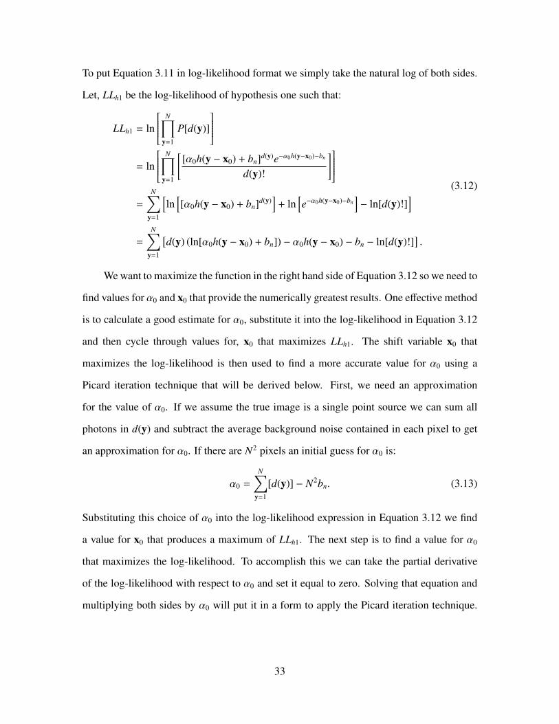
To put Equation 3.11 in log-likelihood format we simply take the natural log of both sides.
Let, LLh1 be the log-likelihood of hypothesis one such that:
LLh1 = ln
N∏y=1
P[d(y)]
= ln
N∏y=1
[[α0h(y − x0) + bn]d(y)e−α0h(y−x0)−bn
d(y)!
]=
N∑y=1
[ln
[[α0h(y − x0) + bn]d(y)
]+ ln
[e−α0h(y−x0)−bn
]− ln[d(y)!]
]=
N∑y=1
[d(y) (ln[α0h(y − x0) + bn]) − α0h(y − x0) − bn − ln[d(y)!]
].
(3.12)
We want to maximize the function in the right hand side of Equation 3.12 so we need to
find values for α0 and x0 that provide the numerically greatest results. One effective method
is to calculate a good estimate for α0, substitute it into the log-likelihood in Equation 3.12
and then cycle through values for, x0 that maximizes LLh1. The shift variable x0 that
maximizes the log-likelihood is then used to find a more accurate value for α0 using a
Picard iteration technique that will be derived below. First, we need an approximation
for the value of α0. If we assume the true image is a single point source we can sum all
photons in d(y) and subtract the average background noise contained in each pixel to get
an approximation for α0. If there are N2 pixels an initial guess for α0 is:
α0 =
N∑y=1
[d(y)] − N2bn. (3.13)
Substituting this choice of α0 into the log-likelihood expression in Equation 3.12 we find
a value for x0 that produces a maximum of LLh1. The next step is to find a value for α0
that maximizes the log-likelihood. To accomplish this we can take the partial derivative
of the log-likelihood with respect to α0 and set it equal to zero. Solving that equation and
multiplying both sides by α0 will put it in a form to apply the Picard iteration technique.
33

First, the partial derivative of the expression in Equation 3.12 with respect to α0 is:
∂
∂α0
ln N∏
y=1
P[d(y)]
=
∂
∂α0
N∑y=1
[d(y) (ln[α0h(y − x0) + bn]) − α0h(y − x0) − bn − ln[d(y)!]
]0 =
N∑y=1
[d(y)h(y − x0)α0h(y − x0) + bn
− h(y − x0) − 0 − 0]].
(3.14)
Again note that the sum over all pixels of the normalized PSF is unity,∑N
y=1 h(y − x0) = 1,
which reduces Equation 3.14 to:
1 =
N∑y=1
[d(y)h(y − x0)α0h(y − x0) + bn
]. (3.15)
If we multiply both sides of Equation 3.15 by α0 we can create an iterative algorithm by
applying the Picard technique. If we let n represent the iteration index, let the left side be
the new α0 such that our final update equation is:
α0(n+1) = α0(n)
N∑y=1
[d(y)h(y − x0)
α0(n)h(y − x0) + bn
]. (3.16)
The initial value for α0(n) is the estimated value found in Equation 3.13. One method
of determining how many iterations to run is to compare the variance between α0(n+1) and
α0(n). Once the difference between the old and new alphas are within a desired value the
iteration process can end. The final value of α0(n+1) from Equation 3.16 along with the
previously calculated value for x0 is entered a final time into the log-likelihood equation
for hypothesis one, in Equation 3.12, to produce the number that will be compared with the
other log-likelihood values from hypothesis zero and two.
The next section will derive the hypothesis two algorithms and follows the
methodology in this section very closely.
3.1.3 Two point source derivation.
The final hypothesis we will look at, hypothesis two, assumes the true image, λ(x),
is two point sources with amplitude α1 and α2 with bn again representing the average
34

background noise described in Section 3.1.2:
λ(x) = α1δ(x − x1) + α2δ(x − x2) + bn. (3.17)
The expected value of the detected image at pixel location y, d(y), can be written as
the discrete convolution of the true image λ(x) with the transfer function, h(y):
E[d(y)] =
N∑x=1
λ(x)h(y − x). (3.18)
Similar to the hypothesis one, substituting the expression in Equation 3.17 into Equation
3.18 and applying the sifting property of a Dirac and noting once again that the sum of the
optical transfer function over all pixels is unity,∑N
y=1 h(y − x0) = 1, gives the following
result:
E[d(y)] = α1h(y − x1) + α2h(y − x2) + bn. (3.19)
Photon arrivals in the detection plane are governed by Poisson statistics. Furthermore,
we assume noise in each pixel in the detection plane is statistically independent. This
allows us to write the joint PMF as:
N∏y=1
P[d(y)] =
N∏y=1
[[α1h(y − x1) + α2h(y − x2) + bn]d(y)e−α1h(y−x1)−α2h(y−x2)−bn
d(y)!
]. (3.20)
As was done for hypothesis one, we will put Equation 3.20 into a log-likelihood format
and simplify. Let LLh2 be the log-likelihood for hypothesis two which is equal to the natural
35

log of Equation 3.20:
LLh2 = ln
N∏y=1
P[d(y)]
= ln
N∏y=1
[[α1h(y − x1) + α2h(y − x2) + bn]d(y)e−α1h(y−x1)−α2h(y−x2)−bn
d(y)!
]=
N∑y=1
ln[[α1h(y − x1) + α2h(y − x2) + bn]d(y)
]+ ln
[e−α1h(y−x1)−α2h(y−x2)−bn
]ln[d(y)!]
=
N∑y=1
[d(y) ln[α1h(y − x1) + α2h(y − x2) + bn] − α1h(y − x1) − α2h(y − x2) − bn
ln[d(y)!]
].
(3.21)
The final result of Equation 3.21 is what will be implemented to calculate the log-likelihood
of hypothesis two. There are four unknown variables needed to find the maximum value
namely the most likely amplitude and pixel location of the hypothesized true image. As
with hypothesis one, we can make a initial guess as to what the amplitude of α1 and α2
might be assuming the image, d(y), contains two source points of light. In Section 3.1.2
we showed that a good estimate is to sum up the photons in the image, d(y) and subtract
off the estimated background noise photons. We can apply this same technique and simply
assume that each point in the binary is equally as bright. During the iteration phase of this
algorithm more accurate values for α1 and α2 will be descended on. So initial values can
be written as:
α1 = α2 =
∑Ny=1[d(y)] − N2bn
2. (3.22)
Lastly we need to calculate an iterative algorithm for computing accurate values of α1
and α2. This can be accomplished using the same method applied to α0, namely looking at
the gradient with respect to α1 and α2. Starting with the partial derivative of Equation 3.21
36
with respect to α1:
0 =∂
∂α1(LLh2) =
∂
∂α1
ln N∏
y=1
P[d(y)]
=∂
∂α1
N∑y=1
[d(y) ln[α1h(y − x1) + α2h(y − x2) + bn] − α1h(y − x1) − α2h(y − x2) − bn
ln[d(y)!]
]
=
N∑y=1
[d(y)h(y − x1)
α1h(y − x1) + α2h(y − x2) + bn− h(y − x1)]
]
=
N∑y=1
[d(y)h(y − x1)
α1h(y − x1) + α2h(y − x2) + bn
]−
N∑y=1
[h(y − x1)
].
(3.23)
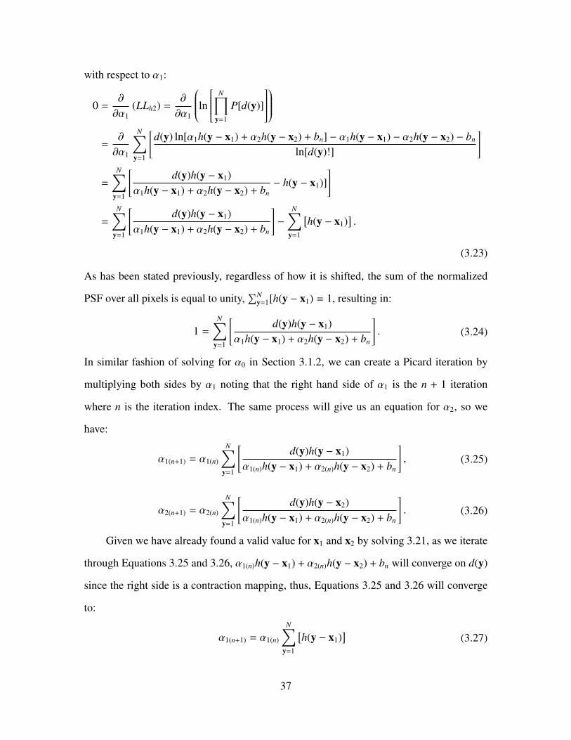
As has been stated previously, regardless of how it is shifted, the sum of the normalized
PSF over all pixels is equal to unity,∑N
y=1[h(y − x1) = 1, resulting in:
1 =
N∑y=1
[d(y)h(y − x1)
α1h(y − x1) + α2h(y − x2) + bn
]. (3.24)
In similar fashion of solving for α0 in Section 3.1.2, we can create a Picard iteration by
multiplying both sides by α1 noting that the right hand side of α1 is the n + 1 iteration
where n is the iteration index. The same process will give us an equation for α2, so we
have:
α1(n+1) = α1(n)
N∑y=1
[d(y)h(y − x1)
α1(n)h(y − x1) + α2(n)h(y − x2) + bn
], (3.25)
α2(n+1) = α2(n)
N∑y=1
[d(y)h(y − x2)
α1(n)h(y − x1) + α2(n)h(y − x2) + bn
]. (3.26)
Given we have already found a valid value for x1 and x2 by solving 3.21, as we iterate
through Equations 3.25 and 3.26, α1(n)h(y − x1) + α2(n)h(y − x2) + bn will converge on d(y)
since the right side is a contraction mapping, thus, Equations 3.25 and 3.26 will converge
to:
α1(n+1) = α1(n)
N∑y=1
[h(y − x1)
](3.27)
37

α2(n+1) = α2(n)
N∑y=1
[h(y − x2)
]. (3.28)
Again, no matter how the normalized PSF, h(y), is shifted around the sum over all pixels
will be unity by definition, thus,∑N
y=1[h(y − x1)
]=
∑Ny=1
[h(y − x2)
]= 1. Once the
difference between the old and new alphas are within a desired value the iterative process
ends and the final log-likelihood can be calculated using the last values of α1(n+1) and α2(n+2)
as well as the x1 and x2 values determined during the first iteration of Equation 3.21 by
plugging all these values back into 3.21. This final log-likelihood value will be compared
with the value found from hypothesis one to make a determination as to weather the image,
d(y) was the result of a single point source or a binary source.
3.2 Software implementation
Software implementation was accomplished using Matlab™. The following subsec-
tions will provide a description of software implementation considerations to maximize
detection while minimizing false alarm rates and processing time.
3.2.1 Point source threshold.
One of the first tests is to determine if an image contains a high enough signal to
noise ratio to be considered for hypothesis one and two. If an image contains no pixels
above a calculated threshold it is ignored from further processing. This threshold is based
on the detected background noise as well as a pre-determined tolerance for false positive
point sources. The probability that a pixel which contains only background noise is falsely
measured as a valid signal is:
Pfalse signal = 1 −t∑
k=0
(bn)ke−bn
k!. (3.29)
For the simulated results provided in this thesis the probability of a false signal was set
to, Pfalse signal = 1 × 10⁻⁸. What remains is to solve for the threshold variable, t such
that the right side of Equation 3.29 is equal to 1 × 10⁻⁸. This is the first threshold used in
implementation and is used for determining which pixels in an image warrant processing.
38

If an image contains no pixels above the threshold, it is determined to be hypothesis zero,
no objects detected.
3.2.2 zero point source implementation.
As soon as the detected image, d(y), is captured, cropped and ready for detection pro-
cessing the median background noise can be calculated. The results for this background
noise estimate, referred to as bn throughout this thesis, are fed into the first threshold dis-
cussed in the previous subsection. If an image to be processed contains no pixels that
exceed the background noise threshold they are ignored and it is assumed that hypothesis
zero is correct. In this way the image does not need to be processed for hypothesis one and
two if it meets the criteria for being hypothesis zero, that is when the image is assumed to
have no point sources.
3.2.3 Single point source implementation.
Given we have already calculated the background noise, bn, and have a valid PSF,
h(y), we can implement the log-likelihood equation for hypothesis one, 3.12, and the α0(n+1)
Equation, 3.16. The results of these two algorithms will be the most likely intensity and
location of a single point source that could produce the detected image, d(y). It will also
produce a numerical value, the log-likelihood, which will be compared to hypothesis two
to determine detection of a binary. As derived in Section 3.1.2, the log-likelihood for
hypothesis one is:
LLh1 =
N∑y=1
[d(y) (ln[α0h(y − x0) + bn]) − α0h(y − x0) − bn − ln[d(y)!]
].
To improve the computational efficiency, the term, ln[d(y)!] is dropped. This will not
impact the final decision because it sums to the same value in both hypothesis one and two.
The final form of LLh1 that will be implemented in code is:
LLh1 =
N∑y=1
[d(y) (ln[α0h(y − x0) + bn]) − α0h(y − x0) − bn
]. (3.30)
39

Given the above information, the implementation process is as follows,
1. Calculate the estimate for α0 using Equation 3.13.
2. Calculate the log-likelihoods for hypothesis one, Equation 3.30, using the estimate
for α0 and cycling through valid source locations governed by x0.
3. Find the x0 associated with the highest log-likelihood value.
4. Use the x0 found in step 3 to find a more accurate value of α0, denoted α0(n+1), where
n is the number of iterations used to converge on a value where α0(n+1) = α0(n) using
Equation 3.16.
5. Using the values of α0(n+1) and x0 calculated above, calculate the log-likelihood of
hypothesis one a final time. This is the value used in comparison with hypothesis
two results.
Not all pixels need to be evaluated as potential locations of the point source, x0. Only pixels
in a 20 by 20 grid surrounding the brightest pixel in a given image, d(y) are evaluated. This
step significantly reduced the processing time.
3.2.4 Two point source implementation.
Implementation of the binary or two point source hypothesis is similar to hypothesis
one. It is worth repeating for completeness. Given the background noise, bn, and valid
PSF, h(y), we can implement hypothesis two log-likelihood Equation 3.21, as well as the
α1(n+1) and α2(n+1) Equations 3.27 and 3.28. As derived in Section 3.1.3, the log-likelihood
for hypothesis two is:
LLh2 =
N∑y=1
[d(y) ln[α1h(y − x1) + α2h(y − x2) + bn] − α1h(y − x1) − α2h(y − x2) − bn
ln[d(y)!]
].
To improve the computational efficiency, the term, ln[d(y)!] is dropped. This will not
impact the final decision because it sums to the same value in hypothesis zero, one and
40

two. The final form of LLh2 that will be implemented in code is:
N∑y=1
[d(y) ln[α1h(y − x1) + α2h(y − x2) + bn] − α1h(y − x1) − α2h(y − x2) − bn
]. (3.31)
Given the above information, the implementation process is the same as hypothesis one the
primary difference being the need to solve for two point source intensities and locations
instead of one. The process is as follows,
1. Calculate the estimate for α1 and α2 using Equation 3.22.
2. Calculate the log-likelihoods for hypothesis two, Equation 3.31, using the estimates
for α1 and α2 from step one and cycling through valid source locations governed by
x1 and x2. This requires a quadruple iteration loop.
3. Find the x1 and x2 associated with the highest log-likelihood value.
4. Use the x1 and x2 found in step three to find a more accurate value of α1 and α2,
denoted α1(n+1) and α2(n+1), where n is the number of iterations used to converge on a
value where α1(n+1) = α1(n) and α2(n+1) = α2(n)using Equation 3.27 and Equation 3.28.
5. Using the values of α1(n+1) and α2(n+1) from step four and x1 and x2 from step three,
calculate the log-likelihood of hypothesis two one final time. This is the value used
in comparison with hypothesis one results.
Again, not all pixels need to be evaluated as potential locations of the point sources, x1 and
x2. Only pixels in a 20 by 20 grid surrounding the brightest pixel in a given image, d(y)
are evaluated. In addition, pixel locations in the subset that did not exceed the estimated
background noise were ignored. These steps significantly reduced the processing time.
3.2.5 Decision process.
It is important to note that all simulated tests used short exposure generated images
for both the detected image and the PSF. The measured images used are long exposure
41

images. An area for further testing is to compare detection techniques using simulating
long exposure images in various configurations.
Given the log-likelihood values found from implementing the hypothesis one and two
algorithms, the task of making a correct decision is the next step. One would think that
simply comparing the results would give the best decision as to weather or not a binary
exists. However, because hypothesis two has more degrees of freedom its log-likelihood
value is almost always higher than hypothesis one. A bias is needed to give more weight
to hypothesis one. If τ is the bias, the following equation demonstrates the decision logic
implemented in simulation:
LLH2 > LLH1 + τ. (3.32)
Finding the value for τ that increases the probability of correct detection and reduces the
probability of false alarm is a key point of the simulation tests. Chapter four will provide
the results of several tests that show how properly choosing τ can impact false alarm and
detection requirements.
Another important decision criteria is how close can two objects be in the detection
plane and be considered two objects. Some deep space surveillance telescopes are under
sampled. A single object that is smaller than a pixel in the detection plane might appear
as two adjacent pixels due to atmospheric blurring or the orientation of the telescope. For
this reason, the detection code will ignore the eight pixels immediately surrounding the
brightest pixel in the area of interest. If this step is not done, the Probability of False
Alarm (P f a) rate goes up to around 40% due to the single point source often being split
between two adjacent pixels as described. This pixel elimination induces a requirement
that a binary will only be detected if there is at least one pixel of separation between the
point sources. This may not be necessary depending on the image quality. For instance,
this restriction was not needed on the measured images used in this thesis. An area of future
research is to explore using sub-pixel processes to allow binaries to be detected with high
42

confidence when two bright pixels are adjacent.
Applying the bias correction τ and adjacent pixel restriction as described above, the
final step is to compare the log-likelihoods. The most likely hypothesis is returned as
the final decision of the code. Chapter four will show a number of results using various
initial conditions. The next section will discuss how the simulations for those results were
conducted.
The detection technique used for the images processed by the correlation method
took the brightest pixel and then, based on it’s intensity, looked for another pixel with
brightness above a variable threshold. The threshold for the second pixel was determined
by keeping the false alarm rate below 10%. Again, the restriction on adjacent pixels being
valid solutions was enforced.
3.3 Simulation test model
An in-focus telescope was simulated to test various seeing parameters and thresholds
using the multi-hypothesis implementation previously described. The diameter, D, and
focal length are 1 meter. The detection plane consisted of N × N samples, where N = 128.
The wavelength of light, λ, was set to, λ = 0.5 µm. Photon arrival is assumed to be
governed by Poisson statistics and is applied to the intensities calculated at each point in the
detection plane. As with most simulated tests, the number of trials is important. For each of
the simulated test, 200 random images were generated for each background noise, seeing
condition, and binary/point source intensity. The next few subsections will provide more
detail on atmospheric settings, how the threshold, source intensities, and seeing conditions
were simulated, and how results were quantified.
3.3.1 Modeling atmospheric effects.
As described in Section 2.1.1, randomly generated phase screens using Zernike
polynomials were used for all simulation models. Again, as was previously described,
given an aperture diameter, D, Fried seeing parameter, r0, and how many polynomial
43

expansions are desired, a random phase screen can be produced using Equations 2.1-
2.9 found in Chapter 2. The number of Zernike polynomials used will dictate the
amount of higher order aberrations that the model will be able to reproduce. For
the simulations conducted for this thesis 85 Zernike polynomials were used to model
atmospheric distortion. The diameter of the aperture was set to, D = 1 meter. The Fried
seeing parameter, r0, is one of the variables modulated during different tests, the results of
which are provided in Chapter 4.
3.3.2 Test variables.
For the simulated binary tests, two point sources were modeled being separated by the
equivalent of one pixel in the detection plane. The parameters for the tests were as follows,
1. The Fried seeing parameter, r0. Adjusting this directly influences the amount of
atmospheric turbulence created by the Zernike phase screen generator. A larger
r0, given in meters, corresponds with better seeing conditions and thus lower
atmospheric turbulence.
2. Switching between one or two point sources to demonstrate both correctly detecting
when two point sources are present and also properly detecting when only a single
point source was simulated.
3. Point source intensity and intensity variance between binary points. Both the overall
intensity and the intensity between the two point sources was modulated to show
performance falloff and error rates as light levels drop and/or light variance increases
between points.
These three items–seeing conditions, a single vs. binary source, and light intensity for the
source(s) were the only variables changed to produce the simulated images used for testing.
The only variable in the detection phase of the code is τ, which controls the weighted bias
for hypothesis one to counteract the advantage hypothesis two has in degrees of freedom.
44

3.3.3 Performance measurements for simulated data.
By adjusting the three variables described in the previous section, namely, seeing
conditions, one or two point sources, and source intensity, simulated single-frame short
exposure images are produced. The multi-hypothesis algorithm processes these simulated
images and produces log-likelihoods for hypothesis one and two. A decision is then made
as to which hypothesis is more likely. Two key metrics are Probability of False Alarm, P f a,
and Probability of Detection, PD. The results found in Chapter 5 will show plots for the
probabilities of detection and false alarm as these different variables are adjusted. The goal
is to form conclusions on what kind of performance can be expected given different source
patterns in various seeing conditions.
3.3.4 Simulated comparison model.
In an effort to show how image reconstruction techniques might perform in the same
simulations, an imaging by correlation process with its corresponding result data has been
implemented. The simulated images are the same as for the multi-hypothesis model. For
detection, a simple logic process is used to decide if the reconstructed image contains one
or two objects in the area of interest above a threshold set to reduce the false alarm rate.
Similar to the multi-hypothesis method, pixels immediately surrounding the brightest pixel
in the region of interest are ignored to lower the false alarm rate considerably. The imaging
by correlation technique implemented is outlined in Chapter 2 Section 2.1.3. Because the
simulation tests a single short exposure image, the intensity of the source is increased to
allow the imaging by correlation method to get into a range in which it can reconstruct
a binary. Another note is the use of a low D/r0 value, it was also necessary to lower
this value to obtain reasonable results. The imaging by correlation method typically uses
multiple images of the same object to achieve quality results. However, to compare it to
the multi-hypothesis method, which in these simulations only use single short exposure
45

images, atmospheric effects are reduce to compensate for lack of multi-frame imaging.
The low D/r0 can be effectively achieved by an adaptive optic system.
3.4 Measured data test model
A large data set of images taken of various geosynchronous objects by the Space
Surveillance Telescope (SST) is examined in this section. In some of the images, it is clear
that a dim star moves close to the stationary object–even where they appear to be a single
object. This provides a good set of images to demonstrate potential real-world performance
of the multi-hypothesis detection algorithms. The measured data test follows these steps,
1. import measured data image to be processed for detection
2. import measured data images to be used to calculate estimated PSF
3. Calculate estimate PSF based on images of a single point taken near to the time and
location of the image to be processed for detection.
4. Calculate the estimate background noise level of the image to be processed for
detection.
5. process the image for detection through the multi-hypothesis algorithm. Return the
log-likelihood of both hypothesis one and two.
The results of this process for the images previously described are provided in Chapter 4.
3.4.1 Description of measured data.
The measured data used in this test was taken by the SST, which is a Defense
Advanced Research Projects Agency (DARPA) program designed to detect space debris
in earth’s orbit (see http://www.darpa.mil/Our Work/TTO/Programs/Space Surveillance
Telescope (SST).aspx for more information). The images used in this thesis were taken
in 2012 and focus on the ANIK-F1 and ANIK-F1R geosynchronous communications
satellites.
46

3.4.2 Deriving a valid PSF.
As enumerated above, a valid PSF is key to estimating the most likely location and
intensity of the point source(s). This is done by taking multiple images at around the
same time and location as the image being processed for detection. The average PSF over
these multiple images is when running the multi-hypothesis algorithm. One of the major
assumptions of this method is the ability to obtain a valid point spread function.
3.4.3 Determining success of measured data test.
The set of images used for this test shows a satellite in the center while a dim star
moves into the picture and eventually right next to the satellite. The detection algorithm
should properly detect the single object until the second object, the star, moves into the
region of interest. How well it performs when the satellite and the star look like a single
point is of particular interest. The results of this test are reported in Chapter 4.
47

IV. Results
The goal of this chapter is to provide test results using both simulated and measured
data in a way that is easy to compare and digest. Please refer to Chapter 3 of this
thesis for a more detailed look at the setup of the simulations. The basic simulation setup
is to generate images using phase screens to represent various amounts of atmospheric
distortion on binary points separated by a single pixel width. Average background noise
and atmospheric turbulence are varied by noted amounts in each section. The first section
will look at the relationship between the Probability of Detection (PD) and P f a as governed
by a bias variable. The second section will compare the multi-hypothesis method to an
implementation of imaging by correlation as described in Chapter 3. The third section will
look at results as real measured images are evaluated by the multi-hypothesis detection
algorithm.
4.1 Multi-hypothesis binary detection simulation results
Test parameters for calculating the PD and P f a are as follows,
1. Three different binary sources were used. All with a detection-plane pixel-width of
separation between points.
A. First, both points at 500 photons of intensity.
B. Second, one point source at 1000 and one at 500 photons of intensity.
C. Third, both points at 1000 photons of intensity.
2. Three different point sources were used to measure P f a related to the PD of similar
intensity.
A. First, a single point at 1000 photons of intensity corresponding to the binary
points of 500 photons each.
48

B. Second, a single point at 2000 photons of intensity corresponding with the
binary points of 1000 photons each.
C. Third, a single point at 1500 photons each corresponding with the binary
points of 1000 and 500.
3. 200 random images were generated for each binary source for each combination of
D/r0 and background noise level.
4. D/r0 levels simulated, D/r0 = [1.25, 1.43, 1.67, 2, 2.5, 3.33, 5, 10].
5. Background levels simulated, noise = [1, 2, 3, 4, 5, 6, 7, 8] photons.
6. The center of mass of each simulated image was centered and a pixel window of
128x128 was sent to the algorithm for processing.
7. A normalized PSF was simulated corresponding to each simulated image passing
through the same atmospheric phase screen.
8. The assumption that there must be at least one pixel of separation between the binary
points was enforced in the code, so adjacent pixels were not considered as valid
hypothesis two solutions. This reduces the false alarm rate.
It should be noted that the decision to use Freid seeing parameters above 0.3m is made to
simulate conditions when atmospheric distortion is justified by the effect of adaptive optics
which partially compensate for the effects of atmospheric turbulence.
49

4.1.1 Image generation.
The following are a sample of the 76,800 images generated and processed to estimate
the probability of detection and false alarm for various noise and seeing conditions. The
first, Figure 4.1, shows samples of simulated short exposure binaries, the second, Figure
4.2, single point sources. The amount of background noise and atmospheric conditions are
noted under each sample image.
50

(a) D/r0=1.25, b
n=1 (b) D/r
0=1.25, b
n=5 (c) D/r
0=1.25, b
n=8
(d) D/r0=2, b
n=1 (e) D/r
0=2, b
n=5 (f) D/r
0=2, b
n=8
(g) D/r0=3.3, b
n=1 (h) D/r
0=3.3, b
n=5 (i) D/r
0=3.3, b
n=8
(j) D/r0=10, b
n=1 (k) D/r
0=10, b
n=5 (l) D/r
0=10, b
n=8
Figure 4.1: Sample simulated detected images of binary source with 500 photons for each
point. Samples taken for various background noise and D/r0 values as given next to each
image. Zoomed in to 31x31 pixels.
51

(a) D/r0=1.25, b
n=1 (b) D/r
0=1.25, b
n=5 (c) D/r
0=1.25, b
n=8
(d) D/r0=2, b
n=1 (e) D/r
0=2, b
n=5 (f) D/r
0=2, b
n=8
(g) D/r0=3.3, b
n=1 (h) D/r
0=3.3, b
n=5 (i) D/r
0=3.3, b
n=8
(j) D/r0=10, b
n=1 (k) D/r
0=10, b
n=5 (l) D/r
0=10, b
n=8
Figure 4.2: Sample simulated detected images of single point sources used in calculating
false alarm rates. Samples taken for various background noise and D/r0 values as given
next to each image. Zoomed in to a 31x31 pixel area.
52

4.1.2 Log-likelihood bias correction.
Hypothesis two has an advantage in the form of more degrees of freedom to fit two
shifted and scaled point spread functions to the detected image. If LLH1 and LLH2 are the
log-likelihood results of hypothesis one and two respectively then:
LLH2 > LLH1 + τ, (4.1)
where τ is controls how much bias to give to hypothesis one to reduce the false alarm rates.
For the simulation results of this thesis, a maximum false alarm rate of 10% was set and τ
adjusted accordingly. The resulting value for τ for each test is as follows,
1. Test one, binary of 500 photons each and a single point source of 1000 photons.
τ = 36.
2. Test two, binary of 1000 and 500 photons and a single point source of 1500 photons.
τ = 60.
3. Test three, binary of 1000 photons each and a single point source of 2000 photons.
τ = 88.
The next several subsections will provide the resulting PD and P f a tables corresponding
with each test.
4.1.3 Probability of Detection (PD) sample results.
The PD tables in this section provide data on how often the multi-hypothesis
algorithm successfully detected a binary averaged over 200 trials under each combination
of background noise and D/r0. Background noise increases moving vertically and D/r0
increases moving horizontally in each table. Each of the three tables in this section are
from a different combination of binary sources. The first is from a binary whose simulated
intensity at the aperture plane, prior to applying the atmosphere and noise, are each 500
photons. The second is a binary where one point is 1000 and one is 500 photons. The last
table provides the PD results when the binary points each have 1000 photons.
53

Table 4.1: Probability of Detection (PD) results using binary source with 500/500 photons.
PD results, binary source 500/500 photons
atmospheric seeing, D/r0
1.25 1.43 1.67 2.00 2.50 3.33 5.00 10.00
adde
dba
ckgr
ound
nois
ein
phot
ons 1 100% 100% 100% 100% 100% 100% 99.5% 96.5%
2 100% 99.5% 99.5% 98% 92.5% 92% 78.5% 26%
3 93.5% 85% 88.5% 81.5% 67.5% 48% 20% 2.5%
4 38.5% 39.5% 27% 21.5% 12% 8% 2.5% 0%
5 4% 5% 2.5% 1.5% 2% 0.5% 0% 0%
6 0% 0% 0% 0.5% 0% 0% 0% 0%
7 0% 0% 0% 0% 0% 0% 0% 0%
8 0% 0% 0% 0% 0% 0% 0% 0%
54

Table 4.2: Probability of Detection (PD) results using binary source with 1000/500 photons.
PD results, binary source 1000/500 photons
atmospheric seeing, D/r0
1.25 1.43 1.67 2.00 2.50 3.33 5.00 10.00
adde
dba
ckgr
ound
nois
ein
phot
ons 1 100% 100% 100% 100% 100% 100% 100% 97.5%
2 100% 100% 100% 100% 98% 90.5% 67.5% 10.5%
3 97% 95% 92.5% 85% 65.5% 44.5% 8% 0%
4 30% 26.5% 21.5% 15% 9% 2% 0% 0%
5 0% 0% 0% 0% 0% 0% 0% 0%
6 0% 0% 0% 0% 0% 0% 0% 0%
7 0% 0% 0% 0% 0% 0% 0% 0%
8 0% 0% 0% 0% 0% 0% 0% 0%
Table 4.3: Probability of Detection (PD) results using binary source with 1000/1000
photons.
PD results, binary source 1000/1000 photons
atmospheric seeing, D/r0
1.25 1.43 1.67 2.00 2.50 3.33 5.00 10.00
adde
dba
ckgr
ound
nois
ein
phot
ons 1 100% 100% 100% 100% 100% 100% 100% 99%
2 100% 100% 100% 99.5% 100% 97.5% 87% 38%
3 98% 97.5% 97.5% 92% 85.5% 73.5% 31.5% 3.5%
4 71% 64.5% 61% 47% 33% 18.5% 6% 0%
5 9% 4% 4% 6% 5% 0.5% 0% 0%
6 0% 0% 0% 0% 0.5% 0% 0% 0%
7 0% 0% 0% 0% 0% 0% 0% 0%
8 0% 0% 0% 0% 0% 0% 0% 0%
55

4.1.4 Probability of false alarm (P f a) simulation results.
The P f a tests entail processing single point sources at similar intensity to a
corresponding binary sources as described in Chapter 3. A maximum P f a of 10% was
enforced as previously stated. Decreasing the P f a will also decrease the detection rate. The
following three tables will follow the style and format of the PD tables using the same scale
and parameters, the only difference being the actual processed images. The first table will
show P f a results using a point source with 1000 photons of intensity in the aperture plane,
again, prior to diffraction, added noise and atmospheric blurring. The second table will
show results when using a point source of 1500 photons and the final table contains the
results when a point source of 2000 photons was used in image generation.
Table 4.4: Probability of False Alarm (P f a) results using point source with 1000 photons.
P f a results, point source with 1000 photons
atmospheric seeing, D/r0
1.25 1.43 1.67 2.00 2.50 3.33 5.00 10.00
adde
dba
ckgr
ound
nois
ein
phot
ons 1 0% 0% 0.5% 0% 2% 5% 8.5% 8%
2 0% 0% 0% 0% 0% 0.5% 0% 0%
3 0% 0% 0% 0% 0% 0% 0% 0%
4 0% 0% 0% 0% 0% 0% 0% 0%
5 0% 0% 0% 0% 0% 0% 0% 0%
6 0% 0% 0% 0% 0% 0% 0% 0%
7 0% 0% 0.5% 0% 0% 0% 1% 0%
8 0.5% 0% 0.5% 0% 0% 0% 0% 0%
56

Table 4.5: Probability of False Alarm (P f a) results using point source with 1500 photons.
P f a results, point source with 1500 photons
atmospheric seeing, D/r0
1.25 1.43 1.67 2.00 2.50 3.33 5.00 10.00ad
ded
back
grou
ndno
ise
inph
oton
s 1 0% 0% 0% 0% 1% 1.5% 3% 8%
2 0% 0% 0% 0% 0% 0% 0% 0%
3 0% 0% 0% 0% 0% 0% 0% 0%
4 0% 0% 0% 0% 0% 0% 0% 0%
5 0% 0% 0% 0% 0% 0% 0% 0%
6 0% 0% 0% 0% 0% 0% 0% 0%
7 0% 0% 0% 0% 0% 0% 0% 0%
8 0% 0% 0% 0% 0% 0% 0% 0%
Table 4.6: Probability of False Alarm (P f a) results using point source with 2000 photons.
P f a results, point source with 2000 photons
atmospheric seeing, D/r0
1.25 1.43 1.67 2.00 2.50 3.33 5.00 10.00
adde
dba
ckgr
ound
nois
ein
phot
ons 1 0% 0% 0% 0% 0.5% 2% 4% 9%
2 0% 0% 0% 0% 0% 0% 0% 0%
3 0% 0% 0% 0% 0% 0% 0% 0%
4 0% 0% 0% 0% 0% 0% 0% 0%
5 0% 0% 0% 0% 0% 0% 0% 0%
6 0% 0% 0% 0% 0% 0% 0% 0%
7 0% 0% 0% 0% 0% 0% 0% 0%
8 0% 0% 0% 0% 0% 0% 0% 0%
57

4.1.5 PD and P f a result summary.
The PD depends on the log-likelihood of hypothesis two being greater than the log-
likelihood of hypothesis one plus a weighting factor, τ. The weighting factor was set in
such a way that the P f a was kept under 10%, for a given test which cycled through various
background noise and atmospheric imaging conditions. The results of this section show
that this multi-hypothesis algorithm can correctly detect binaries under a wide range of
conditions while maintaining a low false alarm rate. However, as seeing conditions fall
below D/r0 = 5 and noise values rise above Bnoise = 4 photons, the detection under these
simulated binaries drops off. As expected, the higher the signal to noise the better overall
detection. The tests where a binary with 1000 and 500 photons of intensity was used show
that the multi-hypothesis algorithm can differentiate a dim object next to a brighter object.
These results also demonstrate that using adaptive optics and/or image post-processing
enhancements that lower the effective D/r0 and raise the signal to noise ratio will greatly
improve the detection rate while maintaining a low false alarm rate. The next section will
compare some of the results above to a detection algorithm used on images enhanced using
speckle interferometry.
4.2 Comparison with imaging by correlation technique
This section will describe the results obtained when running binary and single
point images with various amounts of noise and atmospheric blur through the detection
algorithms as described in Chapter 3. The imaging by correlation technique attempts to
reconstruct the single short exposure image around a small group of pixels that should
contain either a binary or point source. Then a threshold, which has been set to maintain
a false alarm rate below 10%, determines if a binary or single point is contained in the
reconstructed image. This is compared to the multi-hypothesis method which calculates
the log-likelihoods of a single point or binary in a given image. Both methods keep the P f a
below 10% and both enforce the requirement that a binary have at least one pixel of space
58

between points.
The following are the simulation parameters used in the comparison tests.
1. Three different binary sources were used. All with a pixel-width (in the aperture
plane) of separation between points before diffraction and atmospheric blurring.
A. First, both points at 500 photons of intensity.
B. Second, one point at 1000 and one at 500 photons of intensity.
C. Third, both points at 1000 photons of intensity.
2. Three different point sources were used to measure P f a related to the PD of similar
intensity.
A. First, a single point at 1000 photons of intensity corresponding to the binary
points of 500 photons each.
B. Second, a single point at 1500 photons of intensity corresponding with the
binary points of 1000 and 500 photons.
C. Third, a single point at 2000 photons of intensity corresponding with the
binary points of 1000 photons each.
3. 200 random images were generated for each binary source for each combination of
D/r0 and background noise level.
4. D/r0 levels simulated, D/r0 = [1.7, 2.5, 5].
5. Background levels simulated, noise = [1, 2, 3] photons.
6. Images were 128x128 pixels each.
7. A normalized PSF was simulated corresponding to each simulated image passing
through the same atmospheric phase screens.
59

8. The assumption that there must be at least one pixel of separation between the binary
points was enforced in the code.
The next subsections will provide the P f a results first and then the PD results.
4.2.1 Probability of False Alarm (P f a) comparison results.
First the P f a comparison results are provided. As has been mentioned before, a ceiling
of 10% was enforced. The following three figures will show the P f a as a function of D/r0
for the different background noise level as well as for each simulated brightness level.
2 3 4 5
0
0.2
0.4
0.6
0.8
1
D/r0
Pro
b. o
f Fal
se A
larm
(P
FA
)
(a) PFA vs D/r0Background Noise=1
1000 photon point source
MH PFACorr PFA
2 3 4 5
0
0.2
0.4
0.6
0.8
1
D/r0
Pro
b. o
f Fal
se A
larm
(P
FA
)
(b) PFA vs D/r0Background Noise=2
1000 photon point source
MH PFACorr PFA
2 3 4 5
0
0.2
0.4
0.6
0.8
1
D/r0
Pro
b. o
f Fal
se A
larm
(P
FA
)
(c) PFA vs D/r0Background Noise=3
1000 photon point source
MH PFACorr PFA
Figure 4.3: False Alarm rate versus D/r0 for a point source with an intensity of 1000
photons for, (a) background noise level=1, (b) background noise level=2, (c) background
noise level=3.
60

2 3 4 5
0
0.2
0.4
0.6
0.8
1
D/r0
Pro
b. o
f Fal
se A
larm
(P
FA
)(a) PFA vs D/r0
Background Noise=11500 photon point source
MH PFACorr PFA
2 3 4 5
0
0.2
0.4
0.6
0.8
1
D/r0
Pro
b. o
f Fal
se A
larm
(P
FA
)
(b) PFA vs D/r0Background Noise=2
1500 photon point source
MH PFACorr PFA
2 3 4 5
0
0.2
0.4
0.6
0.8
1
D/r0
Pro
b. o
f Fal
se A
larm
(P
FA
)
(c) PFA vs D/r0Background Noise=3
1500 photon point source
MH PFACorr PFA
Figure 4.4: False Alarm rate versus D/r0 for a point source with an intensity of 1500
photons for, (a) background noise level=1, (b) background noise level=2, (c) background
noise level=3.
2 3 4 5
0
0.2
0.4
0.6
0.8
1
D/r0
Pro
b. o
f Fal
se A
larm
(P
FA
)
(a) PFA vs D/r0Background Noise=1
2000 photon point source
MH PFACorr PFA
2 3 4 5
0
0.2
0.4
0.6
0.8
1
D/r0
Pro
b. o
f Fal
se A
larm
(P
FA
)
(b) PFA vs D/r0Background Noise=2
2000 photon point source
MH PFACorr PFA
2 3 4 5
0
0.2
0.4
0.6
0.8
1
D/r0
Pro
b. o
f Fal
se A
larm
(P
FA
)
(c) PFA vs D/r0Background Noise=3
2000 photon point source
MH PFACorr PFA
Figure 4.5: False Alarm rate versus D/r0 for a point source with an intensity of 2000
photons for, (a) background noise level=1, (b) background noise level=2, (c) background
noise level=3.
61

4.2.2 Probability of Detection (PD) comparison results.
This subsection provides the PD comparison results. Each figure plots the probability
of detection versus D/r0 for various background noise and brightness levels as indicated in
each graph. These detection rates are impacted by maximum allowable false alarm rate, as
explained in Chapter 3.
2 3 4 5
0
0.2
0.4
0.6
0.8
1
D/r0
Pro
b. o
f Det
ectio
n (P
D)
(a) PD vs D/r0Background Noise=1
500/500 photon binary source
MH PD
Corr PD
2 3 4 5
0
0.2
0.4
0.6
0.8
1
D/r0
Pro
b. o
f Det
ectio
n (P
D)
(b) PD vs D/r0Background Noise=2
500/500 photon binary source
MH PD
Corr PD
2 3 4 5
0
0.2
0.4
0.6
0.8
1
D/r0
Pro
b. o
f Det
ectio
n (P
D)
(c) PD vs D/r0Background Noise=3
500/500 photon binary source
MH PD
Corr PD
Figure 4.6: Detection rate versus D/r0 for a binary source with an intensities of 500 and 500
photons for, (a) background noise level=1, (b) background noise level=2, (c) background
noise level=3.
62

2 3 4 5
0
0.2
0.4
0.6
0.8
1
D/r0
Pro
b. o
f Det
ectio
n (P
D)
(a) PD vs D/r0Background Noise=1
1000/500 photon binary source
MH PD
Corr PD
2 3 4 5
0
0.2
0.4
0.6
0.8
1
D/r0
Pro
b. o
f Det
ectio
n (P
D)
(b) PD vs D/r0Background Noise=2
1000/500 photon binary source
MH PD
Corr PD
2 3 4 5
0
0.2
0.4
0.6
0.8
1
D/r0
Pro
b. o
f Det
ectio
n (P
D)
(c) PD vs D/r0Background Noise=3
1000/500 photon binary source
MH PD
Corr PD
Figure 4.7: Detection rate versus D/r0 for a binary source with an intensities of 1000
and 500 photons for, (a) background noise level=1, (b) background noise level=2, (c)
background noise level=3.
2 3 4 5
0
0.2
0.4
0.6
0.8
1
D/r0
Pro
b. o
f Det
ectio
n (P
D)
(a) PD vs D/r0Background Noise=1
1000/1000 photon binary source
MH PD
Corr PD
2 3 4 5
0
0.2
0.4
0.6
0.8
1
D/r0
Pro
b. o
f Det
ectio
n (P
D)
(b) PD vs D/r0Background Noise=2
1000/1000 photon binary source
MH PD
Corr PD
2 3 4 5
0
0.2
0.4
0.6
0.8
1
D/r0
Pro
b. o
f Det
ectio
n (P
D)
(c) PD vs D/r0Background Noise=3
1000/1000 photon binary source
MH PD
Corr PD
Figure 4.8: Detection rate versus D/r0 for a binary source with an intensities of 1000
and 1000 photons for, (a) background noise level=1, (b) background noise level=2, (c)
background noise level=3.
63

4.2.3 Comparison result summary.
From the data obtained from the simulation tests, the P f a performance of the imaging
by correlation and multi-hypothesis methods are similar. This is due to the enforcement of
a common maximum of 10% being enforced on both detection algorithms. The maximum
threshold can obviously be increased or decreased depending on the desired false alarm
rate.
Looking at the PD results, it is clear that the multi-hypothesis method, in the given
simulated tests, is superior in detection. These positive results demonstrate a significant
potential improvement over traditional binary detection methods when that detection is
based on a single short exposure image.
4.3 Measured data processing results
As described in Chapter 3, image data was obtained from the DARPA SST. These
images were focused on two satellites in Geostationary Earth Orbit (GEO). As the
telescope is focused on a satellite in GEO, stars appear to pass by in the background. On
a few occasions, a starlight will be right next to the satellite so as to appear to be a single
blurry object. This is the scenario that was run through the multi-hypothesis algorithm to
see if it correctly detected a single source when the object satellite is the only light source
in the frame and then correctly detect a binary as relatively equal intensity starlight moves
into the frame and then right next to the satellite. A PSF was estimated by averaging several
images where a single point is present around the same time as the images processed for
detection. The following four subsections provide the images used and the detection results.
4.3.1 First image: two points spaced far away.
The first image in this sequence of four contains a satellite centered and a star entering
the frame on the top. This is clearly a binary and, as expected, hypothesis two had a higher
log-likelihood.
64

(a) Detected SST Image20x20 pixel area of interest
5 10 15 20
5
10
15
20
400
500
600
700
800
900
1000
(b) Hypothesis 1Reconstructed image
based on log−likelihood reuslts
5 10 15 20
5
10
15
20 0
500
1000
1500
2000
2500
3000
(c) Hypothesis 2Reconstructed image
based on log−likelihood results
5 10 15 20
5
10
15
20
500
1000
1500
2000
2500
3000
Figure 4.9: First measured image (a) Detected image, (b) Result of hypothesis one, (c)
Result of hypothesis two. The log-likelihood of hypothesis two was larger and therefore a
binary was detected.65

4.3.2 Second image: two points in close proximity.
The second image is of most interest. Here the star from the previous frame has
moved right next to the satellite so it would appear as if they are one bright object. The
multi-hypothesis algorithm successfully determined that this is a binary.
66

(a) Detected SST Image20x20 pixel area of interest
5 10 15 20
5
10
15
20
400
500
600
700
800
900
(b) Hypothesis 1Reconstructed image
based on log−likelihood reuslts
5 10 15 20
5
10
15
20 0
500
1000
1500
2000
2500
3000
3500
4000
(c) Hypothesis 2Reconstructed image
based on log−likelihood results
5 10 15 20
5
10
15
20 0
500
1000
1500
2000
2500
3000
Figure 4.10: First measured image (a) Detected image, (b) Result of hypothesis one, (c)
Result of hypothesis two. The log-likelihood of hypothesis two was larger and therefore a
binary was detected.67

4.3.3 Third image: two points touching.
The third frame in this sequence is a lot like the first, where there are clearly two
binaries in the region of interest. The multi-hypothesis process correctly detected the
binary.
68

(a) Detected SST Image20x20 pixel area of interest
5 10 15 20
5
10
15
20
400
500
600
700
800
900
1000
(b) Hypothesis 1Reconstructed image
based on log−likelihood reuslts
5 10 15 20
5
10
15
20 0
500
1000
1500
2000
2500
3000
(c) Hypothesis 2Reconstructed image
based on log−likelihood results
5 10 15 20
5
10
15
20 0
500
1000
1500
2000
2500
3000
Figure 4.11: Third measured image (a) Detected image, (b) Result of hypothesis one, (c)
Result of hypothesis two. The log-likelihood of hypothesis two was larger and therefore a
binary was detected.69

4.3.4 Fourth image: single point.
The last image in this sequence shows the star has passed out of the region of interest.
Here log-likelihood for hypothesis one should be larger. The result of processing this image
was the log-likelihood of hypothesis two did not detect any combination of two points that
rose above the threshold for detection, so it remained defaulted to zero. Whereas the log-
likelihood of hypothesis one correctly detected the single object.
70

(a) Detected SST Image20x20 pixel area of interest
5 10 15 20
5
10
15
20
400
500
600
700
800
(b) Hypothesis 1Reconstructed image
based on log−likelihood reuslts
5 10 15 20
5
10
15
20 0
500
1000
1500
2000
(c) Hypothesis 2Reconstructed image
based on log−likelihood results
5 10 15 20
5
10
15
20 −1
−0.5
0
0.5
1
Figure 4.12: Forth measured image (a) Detected image, (b) Result of hypothesis one, (c)
Result of hypothesis two. The log-likelihood of hypothesis one was greater and so a binary
was not detected.71

4.3.5 Measured data result summary.
These results demonstrate that the multi-hypothesis algorithm can properly differen-
tiate between a single point source and a binary point source in the images shown above.
The processing time on a laptop with two gigahertz processor running Matlab™was ap-
proximately six milliseconds per image. This also demonstrates the potential to run this
detection algorithm in near-real-time to flag images with potential binaries in an area of
interest. These flagged image locations can then be revisited by higher resolution imaging
if desired.
72

V. Future work
5.1 Summary
Binary detection is an important area of interest both inside and outside the Air Force.
Traditional binary detection at geosynchronous orbiting heights is difficult when objects
are too close and/or blurred by atmospheric effects. Many post processing techniques have
been implemented to enhance the resolution and thereby increase the ability to detect bi-
naries. This thesis has proposed a different approach that focuses instead on assuming an
image contains either zero, one, or two point sources. Based of these hypothesis a log-
likelihood can be calculated which can be used for binary detection.
Chapter two reviewed current binary detection techniques along with a brief intro-
duction about multi-hypothesis testing. Chapter three provided the derivations used in this
thesis along with a description of the simulated and measured tests conducted. Chapter
four provided the test results, comparing an imaging by correlation detection method with
the multi-hypothesis algorithm.
Multi-hypothesis testing capitalizes on the additional data contained in the assump-
tions which form each hypothesis. This additional information allows the derivation of a
binary detection algorithm with positive simulation results when compared with an imaging
by correlation detection method. If an objective of an imaging system is to search for and
identify binaries then implementing a multi-hypothesis algorithm can provide increased
detection performance because of the additional information contained in the hypothesis.
5.2 Future work
This thesis focused on actual image data. An early objective that was not realized
in this research was to use multi-hypothesis testing on the spatial frequency information.
A unique cosine fringe pattern in the spatial frequency information of an image denotes
73

a binary is present. However, sometimes this cosine pattern cannot be seen. Deriving a
multi-hypothesis algorithm that assumes the spatial frequency data was formed by zero,
one, or two point sources could allow better detection than current methods.
Another area of more research is how well this method performs when using multi-
frame imaging techniques. The simulation tests in this thesis used only single short
exposure images. Given the positive performance from these short exposure tests does
create a suspicion that multi-frame imaging techniques will only enhance the performance
even more as noise and atmospheric effects are removed through averaging many frames.
Sub-pixel detection was also not explored. When viewing objects that fit inside a
single pixel in the detection plane, if the object is not centered on the pixel it will split the
photon count into two or more adjacent pixels. Adding a multi-hypothesis binary detection
that accounts for sub-pixel locations is a potential area for more investigation.
In a similar vein, detection of more than two objects might be of interest. Having
hypothesis calculations for zero, one, two, and more than two would allow not only binary
but also cluster detection in a given area of interest. This is also an important part of the
Air Force’s mission for space surveillance.
74

Bibliography
[1] Acton, DS and RC Smithson. “Solar imaging with a segmented adaptive mirror”.Applied optics, 31(16):3161–3169, 1992.
[2] Ayers, GR, MJ Northcott, and JC Dainty. “Knox-Thompson and triple-correlationimaging through atmpshperic turbulence”. JOSA A, 5(7):963–985, 1988.
[3] Bates, RHT. “Astronomical speckle imaging”. Physics Reports, 90(4):203–297, 1982.
[4] Beletic, James W. “Deterministic photon bias in speckle imaging”. OpticsCommunications, 71(6):337–340, 1989.
[5] Campisi, Patrizio and Karen Egiazarian. Blind image deconvolution: theory andapplications. CRC press, 2007.
[6] Charbonneau, David, Timothy M. Brown, David W. Latham, and MIchel Mayor.“Detection of Planetary Transits Across a Sun-like Star”. 529(1):L45, 2000. URLhttp://stacks.iop.org/1538-4357/529/i=1/a=L45.
[7] Collins, Graham P. “Making stars to see stars: DOD adaptive optics work isdeclassified”. Physics Today, 45:17, 1992.
[8] Ealey, Mark A. and John A. Wellman. “Deformable mirrors: design fundamentals,key performance specifications, and parametric trades”. San Diego-DL tentative, 36–51. International Society for Optics and Photonics, 1992.
[9] Foy, R. and A. Labeyrie. “Letter to the Editor Feasibility of adaptive telescope withlaser probe”. Astron. Astrophys, 152:L29–L31, 1985.
[10] Fugate, Robert Q. “Laser beacon adaptive optics”. Optics and Photonics News,4(6):14–19, 1993.
[11] Gardner, Chester S., Byron M. Welsh, and Laird A. Thompson. “Design andperformance analysis of adaptive optical telescopes using lasing guide stars”.78(11):1721–1743, 1990.
[12] Gaskill, Jack D. Linear systems, Fourier transforms, and optics. IET, 1978.
[13] Goodman, J. W. Statistical Optics. Wiley, John and Sons, Inc, New York, NY, 1985.
[14] Goodman, J. W. Introduction to Fourier Optics. Roberts and Company Publishers,Greenwood Village, CO, 2005.
[15] Happer, W., GJ MacDonald, CE Max, and FJ Dyson. “Atmospheric-turbulencecompensation by resonant optical backscattering from the sodium layer in the upperatmosphere”. JOSA A, 11(1):263–276, 1994.
75
[16] Hardy, John W. “Active optics: a new technology for the control of light”.Proceedings of the IEEE, 66(6):651–697, 1978.
[17] Hulburd, Bill. “Segmented mirrors for atmospheric compensation”. 1989 IntlCongress on Optical Science and Engineering, 42–51. International Society forOptics and Photonics, 1989.
[18] Knox, Keith T. and Brian J. Thompson. “Recovery of images from atmosphericallydegraded short-exposure photographs”. The astrophysical journal, 193:L45–L48,1974.
[19] Kundur, Deepa and Dimitrios Hatzinakos. “Blind image deconvolution”. SignalProcessing Magazine, IEEE, 13(3):43–64, 1996.
[20] Labeyrie, Antoine. “Attainment of Diffraction Limited Resolution in LargeTelescopes by Fourier Analysing Speckle Patterns in Star Images”.
[21] Lawrence, TW, DM Goodman, EM Johansson, and JP Fitch. “Speckle imaging ofsatellites at the us air force maui optical station”. Applied optics, 31(29):6307–6321,1992.
[22] Lohmann, Adolf W., Gerd Weigelt, and Bernhard Wirnitzer. “Speckle masking inastronomy: triple correlation theory and applications”. Applied Optics, 22(24):4028–4037, 1983.
[23] Marcy, Geoffrey W., R. Paul Butler, Debra Fischer, Steven S. Vogt, Jack J. Lissauer,and Eugenio J. Rivera. “A Pair of Resonant Planets Orbiting GJ 876”. TheAstrophysical Journal, 556(1):296, 2001. URL http://stacks.iop.org/0004-637X/556/
i=1/a=296.
[24] Matson, Charles L. “Weighted-least-squares phase reconstruction from the bispec-trum”. JOSA A, 8(12):1905–1913, 1991.
[25] Meng, Julian, George JM Aitken, E. Keith Hege, and Jeffrey S. Morgan. “Triple-correlation subplane reconstruction of photon-address stellar images”. JOSA A,7(7):1243–1250, 1990.
[26] Northcott, MJ, GR Ayers, and JC Dainty. “Algorithms for image reconstruction fromphoton-limited data using the triple correlation”. JOSA A, 5(7):986–992, 1988.
[27] Phillips, James D. and Stephen C. Cain. “Joint maximum likelihood estimator forpupil and image plane data”. Optical Engineering, 47(2):026002–026002, 2008.
[28] Ribak, Erez N. “Deformable mirrors”. NATO ASI Series C Mathematical andPhysical Sciences-Advanced Study Institute, 423:149–162, 1994.
[29] Richmond, Richard D. and Stephen C. Cain. Direct-detection LADAR systems. SPIEPress, 2010.
76

[30] Roddier, Nicolas A. “Atmospheric wavefront simulation using Zernike polynomials”.Optical Engineering, 29(10):1174–1180, 1990.
[31] Roggemann, M. C. and B. M. Welsh. Imaging Through Turbulence. CRC Press LLC,Boca Raton, FL, 1996.
[32] Rousset, Gerard. “Wave-front sensors”. Adaptive optics in astronomy, 1:91, 1999.
[33] Schmidt, J. D. Numerical Simulation of Optical Wave Propigation With examples inMATLAB© . SPIE Press, Bellingham, WA, 2010.
[34] Schulz, T. J. and D. L. Snyder. “Image recovery from correlations”. 1992.
[35] Schulz, Timothy J. “Multiframe blind deconvolution of astronomical images”. JOSAA, 10(5):1064–1073, 1993.
[36] Schwartz, C., E. Ribak, and SG Lipson. “Bimorph adaptive mirrors and curvaturesensing”. JOSA A, 11(2):895–902, 1994.
[37] Thompson, Laird A. “Adaptive optics in astronomy”. Physics Today, 47:24, 1994.
[38] Troxel, Steven E., Byron M. Welsh, and Michael C. Roggemann. “Off-axis opticaltransfer function calculations in an adaptive-optics system by means of a diffractioncalculation for weak index fluctuations”. JOSA A, 11(7):2100–2111, 1994.
[39] Troxel, Steven E., Byron M. Welsh, and Michael C. Roggemann. “Anisoplanatismeffects on signal-to-noise ratio performance of adaptive optical systems”. JOSA A,12(3):570–577, 1995.
[40] Tyson, Robert. Principles of adaptive optics. CRC Press, 2010.
77

REPORT DOCUMENTATION PAGE Form ApprovedOMB No. 0704–0188
The public reporting burden for this collection of information is estimated to average 1 hour per response, including the time for reviewing instructions, searching existing data sources, gathering andmaintaining the data needed, and completing and reviewing the collection of information. Send comments regarding this burden estimate or any other aspect of this collection of information, includingsuggestions for reducing this burden to Department of Defense, Washington Headquarters Services, Directorate for Information Operations and Reports (0704–0188), 1215 Jefferson Davis Highway,Suite 1204, Arlington, VA 22202–4302. Respondents should be aware that notwithstanding any other provision of law, no person shall be subject to any penalty for failing to comply with a collectionof information if it does not display a currently valid OMB control number. PLEASE DO NOT RETURN YOUR FORM TO THE ABOVE ADDRESS.
1. REPORT DATE (DD–MM–YYYY) 2. REPORT TYPE 3. DATES COVERED (From — To)
4. TITLE AND SUBTITLE 5a. CONTRACT NUMBER
5b. GRANT NUMBER
5c. PROGRAM ELEMENT NUMBER
5d. PROJECT NUMBER
5e. TASK NUMBER
5f. WORK UNIT NUMBER
6. AUTHOR(S)
7. PERFORMING ORGANIZATION NAME(S) AND ADDRESS(ES) 8. PERFORMING ORGANIZATION REPORTNUMBER
9. SPONSORING / MONITORING AGENCY NAME(S) AND ADDRESS(ES) 10. SPONSOR/MONITOR’S ACRONYM(S)
11. SPONSOR/MONITOR’S REPORTNUMBER(S)
16. SECURITY CLASSIFICATION OF:
a. REPORT b. ABSTRACT c. THIS PAGE
17. LIMITATION OFABSTRACT
18. NUMBEROFPAGES
19a. NAME OF RESPONSIBLE PERSON
19b. TELEPHONE NUMBER (include area code)
Standard Form 298 (Rev. 8–98)Prescribed by ANSI Std. Z39.18
27–03–2014 Master’s Thesis Oct 2013–Mar 2014
Binary Detection using Multi-Hypothesis Log-Likelihood,Image Processing
Gessel, Brent H., Captain, USAF
Air Force Institute of TechnologyGraduate School of Engineering and Management (AFIT/EN)2950 Hobson WayWPAFB, OH 45433-7765
AFIT-ENG-14-M-34
Lt Col Travis BlakeSpace Systems (DARPA/TTO)675 North Randolph StreetArlington, VA 22203-2114(703)812-1963
DARPA/TTO
12. DISTRIBUTION / AVAILABILITY STATEMENT
DISTRIBUTION STATEMENT A:APPROVED FOR PUBLIC RELEASE; DISTRIBUTION UNLIMITED
13. SUPPLEMENTARY NOTES
This work is declared a work of the U.S. Government and is not subject to copyright protection in the United States.
14. ABSTRACT
One of the United States Air Force missions is to track space objects. Finding planets, stars, and other natural andsynthetic objects are all impacted by how well the tools of measurement can distinguish between these objects whenthey are in close proximity. In astronomy, the term binary commonly refers to two closely spaced objects. Splitting abinary occurs when two objects are successfully detected. The physics of light, atmospheric distortion, and measurementimperfections can make binary detection a challenge.Binary detection using various post processing techniques can significantly increase the probability of detection. Thispaper explores the potential of using a multi-hypothesis approach. Each hypothesis assumes one two or no points existsin a given image. The log-likelihood of each hypothesis are compared to obtain detection results. Both simulated andmeasured data are used to demonstrate performance with various amounts of atmosphere, and signal to noise ratios.Initial results show a significant improvement when compared to a detection via imaging by correlation. More work existsto compare this technique to other binary detection algorithms and to explore cluster detection.
15. SUBJECT TERMS
binary detection, image post processing, correlation
U U U UU 90
Dr. Stephen C. Cain (ENG)
(937) 255-3636 x4716 [email protected]
Top Related