


Languages
Pages
Legal


Bill Atwood, Core Meeting, 9-Oct. 2002 GLASGLASTT
1
Finding and Fitting
• A Recast of Traditional GLAST Finding: Combo
• A Recast of the Kalman Filter• Setting the e+e- Energies• Vertexing: How to put the tracks together• Bottom Line: PSF & Aeff

Bill Atwood, Core Meeting, 9-Oct. 2002 GLASGLASTT
2
Strips/Clusters to Space Points
A basic to GLAST is the 3-in-a-row trigger: 3 consecutive X-Y planes firing withina microsecond.
This yields possible space points.
Step one: build an object which can cycle over the allowed X-Y pairing in a givenGLAST measuring layer
a) Ordered just as they come X’s then Y’sb) Ordered with reference to closeness to a given space point
x
y
1 2 3
4 5 6
y
12
34
5
6
Case a) Case b)(x,y) Pointfrom whichto search
(nextHit)
(nearestHit)
Bill Atwood, Core Meeting, 9-Oct. 2002 GLASGLASTT
3
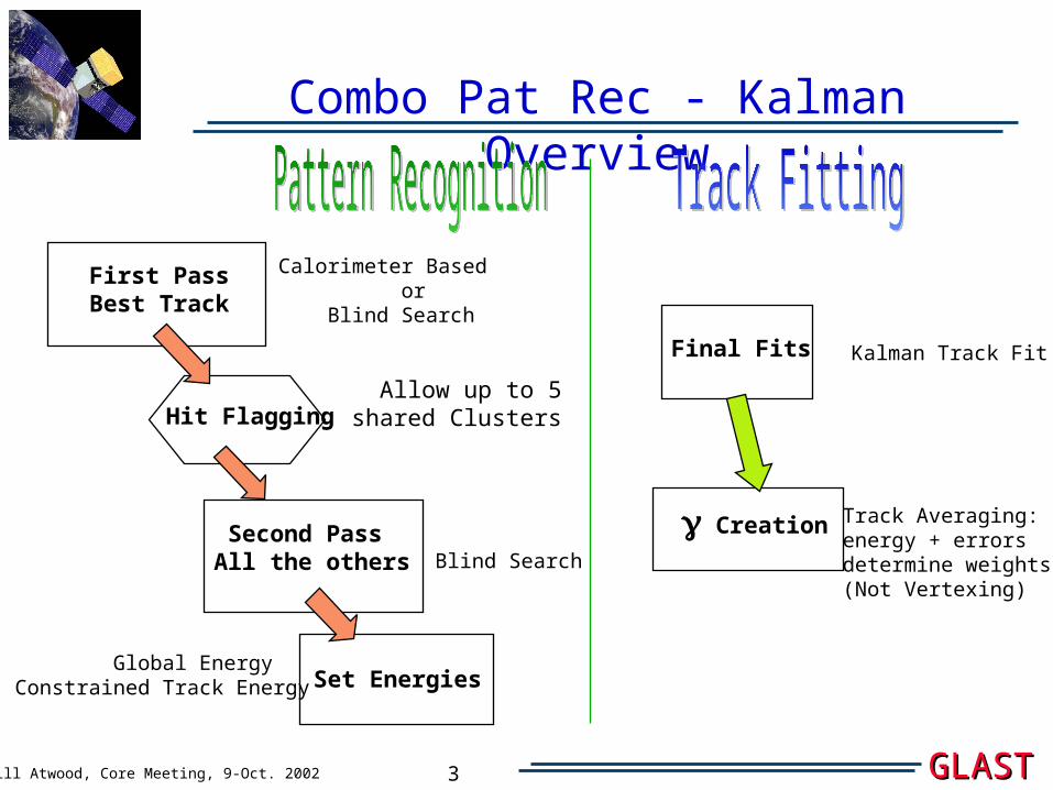
Combo Pat Rec - Kalman Overview
First PassBest Track
Hit Flagging
Second PassAll the others
Set Energies
Final Fits
Creation
Calorimeter Based or Blind Search
Allow up to 5shared Clusters
Blind Search
Global EnergyConstrained Track Energy
Kalman Track Fit
Track Averaging:energy + errorsdetermine weights(Not Vertexing)

Bill Atwood, Core Meeting, 9-Oct. 2002 GLASGLASTT
4
The “Combo” Pat. Rec. (Details)
Starting Layer: One furthest from the calorimeter
Two Strategies: 1) Calorimeter Energy present An energy centroid (space point!)
2) Too little Cal. Energy use only Track Hits
“Combo” Pattern Recognition - Processing an Example Event:
The Event as produce by GLEAM
100 MeV Raw SSD Hits

Bill Atwood, Core Meeting, 9-Oct. 2002 GLASGLASTT
5
The “Combo” Pat. Rec. (Details)
Sufficient Cal. Energy (42 MeV) Use Cal. centroid
Start with hits in outer most layer First Guess: connect hit with Cal. Centroid
Use nearestHit to find 2nd hit

Bill Atwood, Core Meeting, 9-Oct. 2002 GLASGLASTT
6
The “Combo” Pat. Rec. (Details)
Initial Track Guess:Connect first 2 Hits!
Project and AddHits Along the Track within Search Region
The search region is set by propagating the track errorsthrough the GLAST geometry.
The default region is 9 (set very wide at this stage)

Bill Atwood, Core Meeting, 9-Oct. 2002 GLASGLASTT
7
The “Combo” Pat. Rec. (Details)
The Blind Search proceeds similar to the Calorimeter based Search•1st Hit found found - tried in combinatoric order•2nd Hit selected in combinatoric order•First two hits used to project into next layer -•3rd Hit is searched for - •If 3rd hit is found, track is built by “finding - following” as with Calorimeter search
In this way a list of tracks is formed.
Crucial to success, is ordering the list!
(Optimization work still in progress)

Bill Atwood, Core Meeting, 9-Oct. 2002 GLASGLASTT
8
Hit Sharing
Hit Flagging (or Sharing)
In order not to find the same track at most 5 clusters can be shared
The first X and Y cluster (nearest the conversion point) is always allowedto be shared
Subsequent Clusters are shared depending on the cluster width and the track’s slope
Predict 3 hit strips
Observe 5Allow Cluster to be shared
Example of oversized Cluster
Fitted Track
SSDLayer

Bill Atwood, Core Meeting, 9-Oct. 2002 GLASGLASTT
9
Kalman FilterThe Kalman filter process is a successive approximation scheme to estimate parameters
Simple Example: 2 parameters - intercept and slope: x = x0 + Sx * z; P = (x0 , Sx)
Errors on parameters x0 & Sx: covariance matrix: C =
Cx-x Cx-s
Cs-x Cs-s
Cx-x = <(x-xm)(x-xm)> In generalC = <(P - Pm)(P-Pm)T>
Propagation:
x(k+1) = x(k)+Sx(k)*(z(k+1)-z(k))
Pm(k+1) = F(z) * P(k) where
F(z) = 1 z(k+1)-z(k)
0 1
Cm(k+1) = F(z) *C(k) * F(z)T + Q(k)k k+1 Noise: Q(k) (Multiple Scattering)
P(k)Pm(k+1)

Bill Atwood, Core Meeting, 9-Oct. 2002 GLASGLASTT
10
Kalman Filter (2)
Form the weighted average of the k+1 measurement and the propagated track model: Weights given by inverse of Error Matrix: C-1
Hit: X(k+1) with errors V(k+1)
P(k+1) = Cm-1(k+1)*Pm(k+1)+ V-1(k+1)*X(k+1)
Cm-1(k+1) + V-1(k+1)
k k+1 Noise (Multiple Scattering)
and C(k+1) = (Cm-1(k+1) + V-1(k+1))-1
Now its repeated for the k+2 planes and so - on. This is called FILTERING - each successive step incorporates the knowledge of previous steps as allowed for by the NOISE and the aggregate sum of the previous hits.
Pm(k+1)
Bill Atwood, Core Meeting, 9-Oct. 2002 GLASGLASTT
11
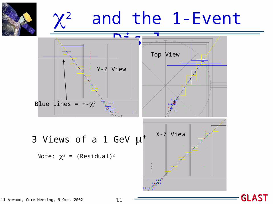
2 and the 1-Event Display
3 Views of a 1 GeV
Blue Lines = +-2
Top View
X-Z View
Y-Z View
Note: 2 = (Residual)2

Bill Atwood, Core Meeting, 9-Oct. 2002 GLASGLASTT
12
<Nhits> = 24 <2> = 1.0/DoF <FIT> = .63 mrad
Use ’s and give the true energy to Kalman Filter
Several Problems discovered During “Sea Trails” Phase•Proper setting of measurement errors •Proper inclusion of energy loss (for ’s - Bethe-Block)•Proper handling of over-sized Clusters
End Results: Example 10 GeV ’s
Kalman Filter: Sea Trials

Bill Atwood, Core Meeting, 9-Oct. 2002 GLASGLASTT
13
Setting the Energies
Track energies are critical in determining the errors (because of the dominance of Multiple Scattering)
A Three Stage Process:
•Kalman Energies: compute the RMS angle between 3D Track segments Key: include material audit and reference energy back to first layer Results: E-Kalman ~ 35% @ 100 MeV (!)
•Determine Global Energy: EGlobal Hit counting + Calorimeter Energy (Resolution limited by Calorimeter response) Results: Depends on Cuts - Best ~ 12% at 100 MeV
•Use Global Energy to Constrain the first 2 track energies: EGolbal = E1Kal + x1*1Kal + E2Kal + x2*2Kal
2 = x12 + x22
Determine x1 & x2 by minimizing 2
The Constrained Energies are then used in the FINAL FIT

Bill Atwood, Core Meeting, 9-Oct. 2002 GLASGLASTT
14
The Final Fits & Creating a
A second pass through the Kalman Fit is done
•Using the Constrained Energies for the First two tracks - others use the default Pat. Rec. energy
•The Track hits are NOT re-found - the hits from the Pat. Rec. stage are used
Creating a (Note this isn’t true “Vertexing”) •Tracks are MS dominated - NOISE Dominated Verticizing - adding NOISE coherently•Use tracks as ~ independent measures of direction•Process:
– Check that tracks “intersect” - simple DOCA Calc.– Estimate Combined direction using Track Errors and Constrained Energies to form the weights

Bill Atwood, Core Meeting, 9-Oct. 2002 GLASGLASTT
15
The Bottom Line: How does it all Work?
Data for 100 MeV, Nrm. Inc.
Thin Section Only - Req. All Events to have 2 Tracks which formed a “vertex” Results: Aeff ~ 3000 cm2
Best Track Resolution: 39 mrad (PSF ~ 3.3 Deg.)
Resolution: 35 mrad (PSF ~ 3.0 Deg)
Difference Plot Shows the Improvement! But… the story is even Better!
Look Ma! NO TAILS!
Bill Atwood, Core Meeting, 9-Oct. 2002 GLASGLASTT
16
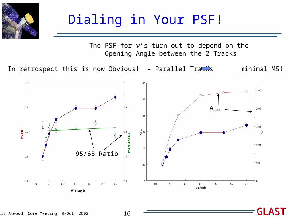
Dialing in Your PSF!
The PSF for ’s turn out to depend on the Opening Angle between the 2 Tracks
In retrospect this is now Obvious! - Parallel Tracks minimal MS!
0.0 0.1 0.2 0.3 0.4 0.5 0.6
VTX Angle
1.5
2.0
2.5
3.0
3.5
PSF6
8
1.0
1.5
2.0
2.5
PSF9
5/PS
F68
0.0 0.1 0.2 0.3 0.4 0.5 0.6
Vtx.Angle
1.5
2.0
2.5
3.0
3.5
4.0
4.5
PSF68
0
500
1000
1500
2000
2500
Aeff
95/68 Ratio
Aeff
Top Related