


Languages
Pages
Legal


Bill Atwood, August, 2003 GLASTGLAST1
Covariance & GLAST
Agenda
• Review of Covariance• Application to GLAST• Kalman Covariance• Present Status

Bill Atwood, August, 2003 GLASTGLAST2
Review of Covariance
ab
Ellipse
12
2
2
2
b
y
a
xTake a circle – scale the x & y axis:
Rotate by : )sin()cos(
)sin()cos(
xyy
yxx
Results:
1))(cos)(sin
()11
)(sin()cos(2))(sin)(cos
(2
2
2
22
222
2
2
22
bay
baxy
bax
Rotations mix x & y. Major & minor axis plus rotation angle complete description.
Error Ellipse described by Covariance Matrix:
n
Distance between a point with an error and another point measured in ’s:
rCrn T 12)( where )( xxr
and
11
111 )(
yyyx
xyxx
CC
CCCInverseC and 11 yxxy CC
Simply weighting the distance by 1/2
Bill Atwood, August, 2003 GLASTGLAST3
Review 2
1211211
1112 2),()(
yyxyxx
yyxy
xyxxT CyxyCCxy
x
CC
CCyxrCrn
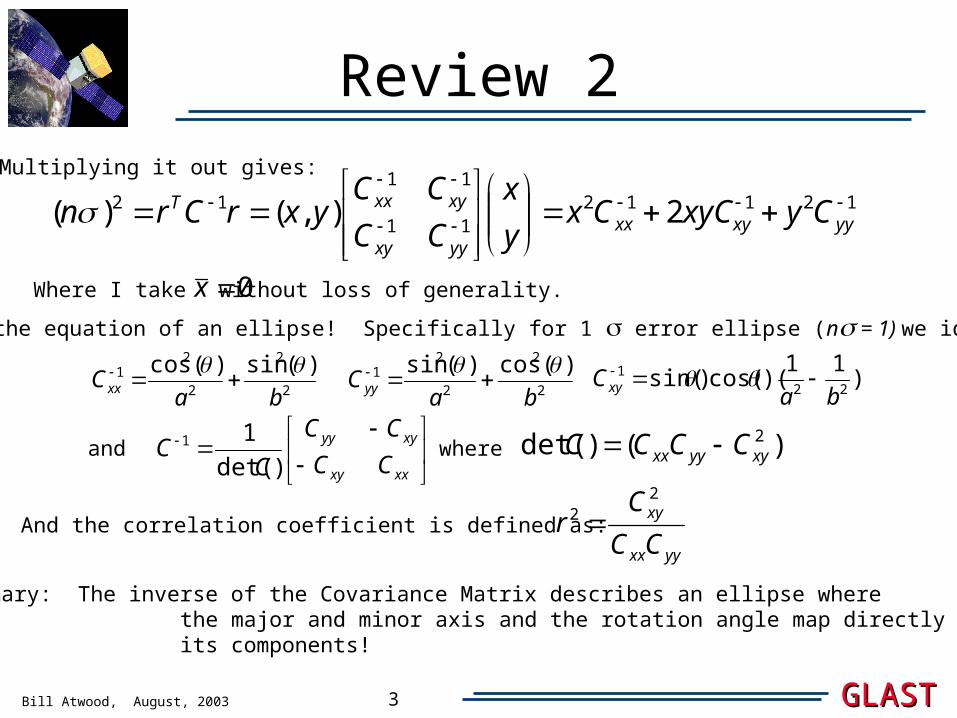
Multiplying it out gives:
Where I take 0x without loss of generality.
This is the equation of an ellipse! Specifically for 1 error ellipse (n = 1) we identify:
2
2
2
21 )(sin)(cos
baCxx
2
2
2
21 )(cos)(sin
baCyy
)
11)(cos()sin(
221
baCxy
and
xxxy
xyyy
CC
CC
CC
)det(
11 where )()det( 2xyyyxx CCCC
Summary: The inverse of the Covariance Matrix describes an ellipse where the major and minor axis and the rotation angle map directly onto its components!
And the correlation coefficient is defined as: yyxx
xy
CC
Cr
22
Bill Atwood, August, 2003 GLASTGLAST4
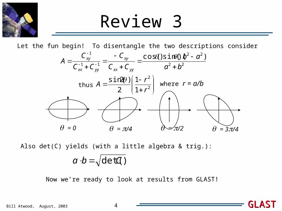
Review 3Let the fun begin! To disentangle the two descriptions consider
22
22
11
1))(sin()cos(
ba
ab
CC
C
CC
CA
yyxx
xy
yyxx
xy
where r = a/b
= 0 = /4 = /2 = 3/4
2
2
1
1
2
)2sin(
r
rA
Also det(C) yields (with a little algebra & trig.):
)det(Cba
Now we’re ready to look at results from GLAST!
thus

Bill Atwood, August, 2003 GLASTGLAST5
Covariance Matrix from Kalman Filter
Results shown for
SYYTkrSXXTkr
SXYTkrAxisAsym
11
1
Binned in cos() and log10(EMC)
Recall however that KF gives us C in terms of the track slopes Sx and Sy.
AxisAsym grows like 1/cos2()
Peak amplitude ~ .4
)1(
)1(
2
1(max)
2
2
r
rA
(max)21
(max)212
A
Ar
3
1
9
1
4.21
4.21
a
br

Bill Atwood, August, 2003 GLASTGLAST6
Relationship between Slopes and Angles
For functions of the estimated variables the usual prescriptions is:
222 )(ivariables
if x
f
when the errors are uncorrelated. For correlated
errors this becomes )()())(( ,,
2
jji
ijij
jiif x
fC
x
f
x
f
x
f
and reduces to the uncorrelated case when jiijiC ,2
,
The functions of interest here are:
221
1)cos(
yx SS and
x
y
S
S)tan(
A bit of math then shows that:
yyxyxx CCC )(sin)cos()sin(2)(cos)(cos 2242
yyxyxx CCC )(cos)cos()sin(2)(sin)(tan
1 222
2
and

Bill Atwood, August, 2003 GLASTGLAST7
Angle Errors from GLASThas a divergence at . However sin() cures this.
decreases as cos2() - while sin() increases as )cos(
1
We also expect the components of the covariance matrix to increase as
due to the dominance of multiple scattering.)cos(
1
log10(EMC)
cos()
Plot measured residuals in terms of Fit 's (e.g. )FIT
MCmeas

Bill Atwood, August, 2003 GLASTGLAST8
Angle Errors 2What's RIGHT: 1) cos() dependence 2) Energy dependence in Multiple Scattering dominated range
What's WRONG: 1) Overall normalization of estimated errors (FIT) - off by a factor of ~ 2.3!!! 2) Energy dependence as measurement errors begin to dominate - discrepancy goes away(?) Both of these correlate with with the fact that the fitted 2's are much larger then 1 at low energy (expected?).
How well does the Kalman Fit PSF model the event to event PSF?

Bill Atwood, August, 2003 GLASTGLAST9
Angle Errors 3 Comparison of
Event-by-Event PSF vs FIT Parameter PSF
(Both Energy Compensated)
Difficult to assess level of correlation - probably not zero - approximately same factor of 2.3

Bill Atwood, August, 2003 GLASTGLAST10
Angle Errors: Conclusions
1) Analysis of covariance matrix gives format for modeling instrument response
2) Predictive power of Kalman Fit?
- Factor of 2.3
- May prove a good handle for CT tree determination of "Best PSF"

Bill Atwood, August, 2003 GLASTGLAST11
Present Analysis Status

Bill Atwood, August, 2003 GLASTGLAST12
Present Status 2: BGE Rejection
Events left after Good-Energy Selection: 1904
Events left in VTX Classes: 26
Events left in 1Tkr Classes: 1878
CT BGE Rejection factors obtained:
20:1 (1Tkr)
2:1 (VTX)
NEED FACTOR OF 10X EVENTS BEFORE PROGRESS CAN BE MADE!
Top Related