


Languages
Pages
Legal

Autonomous Mission Planning and Execution for Unmanned
Surface Vehicles in Compliance with the Marine Rules of the
Road
James Colito
A thesis submitted in partial fulfillment ofthe requirements for the degree of
Master of Science in Aeronautics and Astronautics
University of Washington
2007
Program Authorized to Offer Degree: Aeronautics and Astronautics

University of WashingtonGraduate School
This is to certify that I have examined this copy of a master’s thesis by
James Colito
and have found that it is complete and satisfactory in all respects,and that any and all revisions required by the final
examining committee have been made.
Committee Members:
Rolf Rysdyk
Juris Vagners
Date:


In presenting this thesis in partial fulfillment of the requirements for a master’sdegree at the University of Washington, I agree that the Library shall make its copiesfreely available for inspection. I further agree that extensive copying of this thesis isallowable only for scholarly purposes, consistent with “fair use” as prescribed in theU.S. Copyright Law. Any other reproduction for any purpose or by any means shallnot be allowed without my written permission.
Signature
Date


University of Washington
Abstract
Autonomous Mission Planning and Execution for Unmanned SurfaceVehicles in Compliance with the Marine Rules of the Road
James Colito
Co-Chairs of the Supervisory Committee:Assistant Professor Rolf RysdykAeronautics and Astronautics
Professor Emeritus Juris VagnersAeronautics and Astronautics
In order to achieve a high level of autonomy in a highly dynamic and unpredictable
world, reliable obstacle avoidance is required to ensure the safety of other vessels,
people, and property. Discussed here is the integration of the Coast Guard Interna-
tional Regulations for Avoiding Collision as Sea (COLREGS), or the “Marine Rules
of the Road”, with an autonomous mission management software. The result pro-
vides deliberative obstacle avoidance capability, that complies with the COLREGS,
to an Unmanned Surface Vehicle. The avoidance algorithms are implemented in an
evolutionary path planning system. The planner uses nearby vehicle information and
digital nautical charts to plan compliant paths. Both Head-On and Crossing collision
scenarios are considered. The planner is capable of dynamically replanning paths
based on updated environmental information.

TABLE OF CONTENTS
Page
List of Figures . . . . . . . . . . . . . . . . . . . . . . . . . . . . . . . . . . . iii
Glossary . . . . . . . . . . . . . . . . . . . . . . . . . . . . . . . . . . . . . . . v
Chapter 1: Introduction . . . . . . . . . . . . . . . . . . . . . . . . . . . . 1
1.1 Autonomous Vehicles in a Primarily Human Environment . . . . . . . 1
1.2 State of USV Technology . . . . . . . . . . . . . . . . . . . . . . . . . 2
Chapter 2: USV Guidance, Navigation and Control System . . . . . . . . . 7
2.1 Autonomous Guidance, Navigation and Control System Architecture 7
2.2 Evolution-based Cooperative Planning System (ECoPS) . . . . . . . 10
Chapter 3: Integration of Environmental Information . . . . . . . . . . . . 18
3.1 Adaptation of ECoPS to USVs . . . . . . . . . . . . . . . . . . . . . 18
3.2 Electronic Navigation Charts . . . . . . . . . . . . . . . . . . . . . . 20
3.3 Simulation Results using a Kinematic Model and Digital Elevation Map 20
3.4 Integration of GPS . . . . . . . . . . . . . . . . . . . . . . . . . . . . 21
3.5 Integration of RADAR data . . . . . . . . . . . . . . . . . . . . . . . 24
3.6 Automatic Identification System . . . . . . . . . . . . . . . . . . . . . 26
Chapter 4: Marine Rules of The Road . . . . . . . . . . . . . . . . . . . . . 28
4.1 International Regulations for Avoiding Collisions at Sea . . . . . . . . 30
4.2 Determination of Possible Collision . . . . . . . . . . . . . . . . . . . 33
4.3 Evaluation of Potential Paths to Avoid a Collision . . . . . . . . . . . 37
Chapter 5: Simulation Results . . . . . . . . . . . . . . . . . . . . . . . . . 44
5.1 Simulation Results without Terrain Data . . . . . . . . . . . . . . . . 44
5.2 Elliot Bay Simulation Using Rules of the Road . . . . . . . . . . . . . 48
i

Chapter 6: Conclusion . . . . . . . . . . . . . . . . . . . . . . . . . . . . . 52
Chapter 7: Future Work . . . . . . . . . . . . . . . . . . . . . . . . . . . . 54
Bibliography . . . . . . . . . . . . . . . . . . . . . . . . . . . . . . . . . . . . 56
Pocket Material: CD of Simulation Movies . . . . . . . . . . . . . . . . . . . . 58
ii
LIST OF FIGURES
Figure Number Page
1.1 Examples of Personal Watercraft Size USVs. . . . . . . . . . . . . . . 4
1.2 Examples of Pleasure Craft Size USVs. . . . . . . . . . . . . . . . . . 5
2.1 SEAFOX operated by radio control on Lake Washington, WA. . . . . 8
2.2 Autonomous Guidance, Navigation and Control System Architecture. 9
2.3 Maximizing Utility of Two Distinct Behaviors. . . . . . . . . . . . . . 12
2.4 Example of a Constructed Path. . . . . . . . . . . . . . . . . . . . . . 13
2.5 Evolutionary Process. . . . . . . . . . . . . . . . . . . . . . . . . . . . 13
2.6 Example of Mutate 1-Point Mutation Process. . . . . . . . . . . . . . 16
2.7 Dynamic Path Planning. . . . . . . . . . . . . . . . . . . . . . . . . . 17
3.1 Path Planning System Data Flow. . . . . . . . . . . . . . . . . . . . . 19
3.2 Reconnaissance Mission Simulation Using DEM. . . . . . . . . . . . . 22
3.3 Surveillance Mission Simulation using DEM. . . . . . . . . . . . . . . 23
3.4 Example of a NMEA 0183 Sentence. . . . . . . . . . . . . . . . . . . 25
4.1 Collision Scenario Definition . . . . . . . . . . . . . . . . . . . . . . . 29
4.2 Example of Head-On Passing Behavior. . . . . . . . . . . . . . . . . . 31
4.3 Example of Crossing Behavior. . . . . . . . . . . . . . . . . . . . . . . 32
4.4 Collision Cone Geometry. . . . . . . . . . . . . . . . . . . . . . . . . . 34
4.5 Example of Collision Cone Evaluation Points. . . . . . . . . . . . . . 36
4.6 Active Obstacle Determination for Collision Cone Calculation. . . . . 38
4.7 Process for Evaluating Candidate Plans. . . . . . . . . . . . . . . . . 39
4.8 Evaluation of Head-On Collision Scenario. . . . . . . . . . . . . . . . 42
4.9 Evaluation of Crossing Collision Scenario. . . . . . . . . . . . . . . . 42
5.1 Head-On Collision Simulation With Navigation Rules. . . . . . . . . . 45
5.2 Head-On Collision Without Navigation Rules. . . . . . . . . . . . . . 46
5.3 Crossing Collision With Navigation Rules. . . . . . . . . . . . . . . . 47
iii

5.4 Crossing Collision Without Navigation Rules. . . . . . . . . . . . . . 48
5.5 Head-On Collision Situation in Simulation that Includes DEM. . . . . 50
5.6 Crossing Collision Situation in Simulation that Includes DEM. . . . . 51
5.7 Return to Goal Location in Simulation that Includes DEM. . . . . . . 51
iv
GLOSSARY
AFSL: Autonomous Flight Systems Laboratory
AIS: Automatic Identification System
ARPA: Automatic Radar Plotting Aid
COLREGS: United States Coast Guard International Collision Regulations
DEM: Digital Elevation Map
ECoPS: Evolution-Based Cooperative Planning System
IED: Improvised Explosive Device
ISR: Intelligence Surveillance and Reconnaissance
NGS: National Geospatial-Intelligence Agency
NMEA: National Marine Electronics Association
NMEA 0183: ASCII serial communication protocol, published by NMEA, for com-
munication among marine electronics components.
RIB: Rigged-hull Inflatable Boat
UAV: Unmanned Aerial Vehicle
v
USV: Unmanned Surface Vehicle
UTC: Coordinated Universal Time - Also known as Greenwich Mean Time
UUV: Unmanned Underwater Vehicle
Agent: A member of our team of vehicles.
Collision Cone: A geometric based, mathematical condition, that uses relative motion
of a point and a circle, to determine if a moving point is on a course to intersect
any point in a moving circle.
Committed Trajectory: The waypoints or heading rate commands that have been
sent to the guidance system.
Fitness: A performance measure of how well a path complies with mission objectives.
Port Vector: The vector that points to an obstacle’s port side.
Rule Range: The maximum distance to an obstacle for which we apply the rules of
the road.
Spawn Point: The location the path planner uses for the start of paths. When our
vehicle gets to this location a new trajectory is committed to the guidance
system.
Stern Vector: The vector that points to an obstacle’s stern.
C(Q(sp)): Cost function for a path, Q, from the start point until the endpoint.
∆θ: Difference between heading of our vehicle and that of the obstacle.
vi

J : Objective function for a candidate path.
NT : Number of tasks in a mission scenario.
r: Range to obstacle.
R: Safety radius around the obstacle.
Ri(N): Score of a candidate path from the start point of the path until the endpoint
of the path.
Ri(sp): Score that the vehicle has attained prior to the next spawn point.
Vr: Relative radial velocity
Vθ: Relative angular velocity
αij: Angle between our vehicle location and the obstacles port or stern vector.
n: Number of discretization points on a candidate path.
ψi: vehicle heading
vii

ACKNOWLEDGMENTS
The content of this thesis would not be possible without considerable personal
and technical support from many people. Thanks to my advisors Juris Vagners and
Rolf Rysdyk for their generous support and the opportunity to work on this project.
I’d also like to thank Anawat Pongpunwatta for his patience and technical guidance
in helping me with this work.
Thanks to Chris Lum and the other members of our laboratory.
Thanks to my parents.
I’d especially like to thank Kate Smith for her tremendous support in achieving
this goal. In addition to the occasional grumpy mood she had to endure many nights
and weekends spent working.
Thanks to Bruce Reagan, all of Northwind Marine Inc., and the Washington
Technical Center for their partnership and financial support in this project.
This is part of ongoing research at the University of Washington Autonomous
Flight Systems Laboratory and is only possible as a result of the work of many
students before me.
viii
1
Chapter 1
INTRODUCTION
Unmanned vehicles can serve a wide variety of Intelligence Surveillance and Re-
connaissance (ISR) missions. Benefits to emerging markets such a surveying, research,
search and rescue, and commercial fishing also exist. It is our goal to advance the
current state of USV technology by applying an evolutionary based planning system
to a SEAFOX vessel built by Northwind Marine Inc. The path planning system is
modified to behave according to the marine rules of the road as defined by the Coast
Guard International Regulations for Avoiding Collision as Sea COLREGS [1].
1.1 Autonomous Vehicles in a Primarily Human Environment
In order for the benefits of autonomy to be realized a vehicle must be able to operate
independently of constant operator supervision. The use of a USV presents potential
risk to the safety of others and loss of property. The level of current USV technology
requires constant supervision by operators to ensure avoidance of all obstacles.
One of the more difficult issues related to autonomy is operating in a highly
dynamic environment with other vehicles operated by humans. Humans are capable
of generating some highly unpredictable behaviors. Therefore, an autonomous vehicle
must be flexible enough to deal with unpredictable events or situations and also agile
enough to respond quickly to changing conditions. An evolutionary approach to
path planning is capable of dealing with these unanticipated events in a dynamic
environment.
Obstacle avoidance can be broken into two regimes: near-field or reactive obstacle

2
avoidance and far-field or deliberative obstacle avoidance. This thesis is focused on
developing deliberative obstacle avoidance by using Digital Nautical Map (DEM) and
RADAR information. A method of avoiding collisions with other vehicles according
to the marine rules of the road is described.
The rules of the road are implemented by adapting an evolutionary based path
planning system to, when the circumstances dictate, plan paths according to the
rules of the road. An evolutionary approach is used because many unpredictable
and/or conflicting events can occur in a marine environment. The evolutionary path
planner has the ability to balance these different demands and produce a feasible
path that is free of collisions with other obstacles. The result is a system which
reduces operator workload by autonomously planning paths to meet the demands of
a changing environment.
1.2 State of USV Technology
According to a 2003 USV market survey [2], US Navy planners see USVs as an integral
part of a more agile naval force. A recent Office of Naval Research (ONR) briefing [3]
identified the following benefits,
1. Minimize risk to personnel in high-risk littoral missions.
2. Low cost.
3. Not power limited.
4. Not limited by human factors.
5. Ability to communicate with vehicles both above and below sea.
However, for USVs to be widely accepted technical advances need to be made.
One area where we feel we can contribute is to improve USV autonomy. Typically
3
more than one operator is required to run a single USV, one operator to control the
USV and one to monitor the payload. In order for USVs to be truly efficient one
operator should be able to monitor multiple USVs simultaneously.
The development of USV technology can be dated back to World War II. These
first attempts were primarily designed to be torpedo type vehicles to clear mines
or obstacles in the surf zone. In 1946 USVs were used to collect water samples after
atomic testing on Bikini Atoll. Another common use was (and still is) to use the USVs
as target drone boats for target training purposes [4]. These vessels were typically
operated as radio controlled boats.
Recently, however, the focus has shifted from a simple radio controlled configu-
ration for target practice, to much more complex ISR missions. Attacks on Marine
assets such as USS Cole (2000), French oil Tanker Limburg (2002), Phillippine Su-
perferry 14 (2004), and Khor Al Amaya oil terminal (2004), have driven an increased
interest in anti-terrorism and littoral warfare. The Bush Administrations’ National
Strategy for Maritime Security states that ”infrastructure and systems in the marine
domain... have increasingly become both targets of and potential conveyances for
dangerous and illicit activities.” [5]. According to a recent congressional report [6]
the threat of maritime terrorism is significant and can take many different forms. The
attacks have increased national awareness of maritime security. Increased awareness
coupled with advances in technology have led to a natural increase in attention on
using USV technology for maritime anti-terrorism efforts.
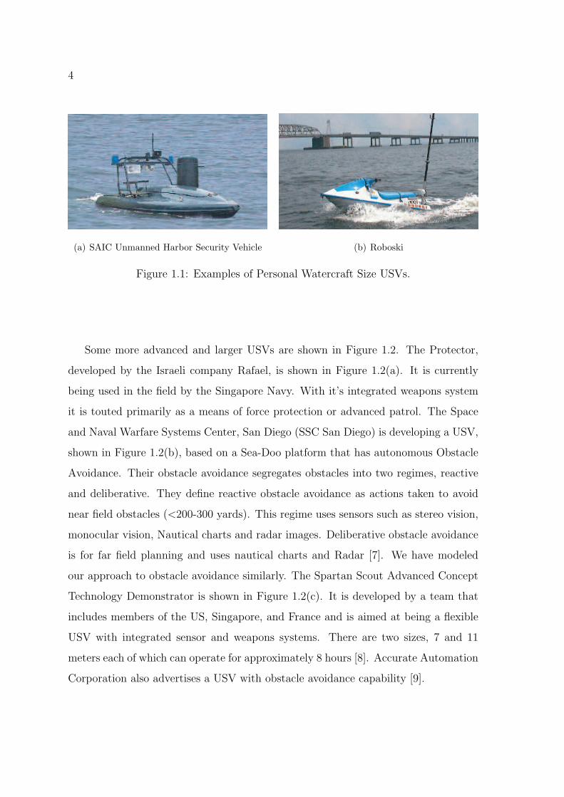
Typical unmanned vessels today are of the pleasure craft size or smaller. Fig-
ure 1.1 shows a couple examples of personal watercraft size USVs. The vehicle shown
in the picture on the left is an advanced version of an earlier USV known as the OWL.
The vehicle shown is developed for port security and offered by Science Application
International Corporation. The Roboski, offered by Robotek Engineering and pic-
tured on the right, was developed to be a low cost, ship deployable target training
device.
4
(a) SAIC Unmanned Harbor Security Vehicle (b) Roboski
Figure 1.1: Examples of Personal Watercraft Size USVs.
Some more advanced and larger USVs are shown in Figure 1.2. The Protector,
developed by the Israeli company Rafael, is shown in Figure 1.2(a). It is currently
being used in the field by the Singapore Navy. With it’s integrated weapons system
it is touted primarily as a means of force protection or advanced patrol. The Space
and Naval Warfare Systems Center, San Diego (SSC San Diego) is developing a USV,
shown in Figure 1.2(b), based on a Sea-Doo platform that has autonomous Obstacle
Avoidance. Their obstacle avoidance segregates obstacles into two regimes, reactive
and deliberative. They define reactive obstacle avoidance as actions taken to avoid
near field obstacles (<200-300 yards). This regime uses sensors such as stereo vision,
monocular vision, Nautical charts and radar images. Deliberative obstacle avoidance
is for far field planning and uses nautical charts and Radar [7]. We have modeled
our approach to obstacle avoidance similarly. The Spartan Scout Advanced Concept
Technology Demonstrator is shown in Figure 1.2(c). It is developed by a team that
includes members of the US, Singapore, and France and is aimed at being a flexible
USV with integrated sensor and weapons systems. There are two sizes, 7 and 11
meters each of which can operate for approximately 8 hours [8]. Accurate Automation
Corporation also advertises a USV with obstacle avoidance capability [9].

5
(a) Protector (b) SSC San Diego USV
(c) Spartan
Figure 1.2: Examples of Pleasure Craft Size USVs.
Another method of pursing autonomy in sea surface vehicles is to develop modular
systems that will work independent of vehicle platform. There is an abundance of
off-the-shelf autopilot products in the marine industry. These products typically offer
waypoint guidance with some “dodge” features where the captain has to manually
tell the autopilot to temporarily change course. These systems all require constant
operator supervision and are not designed for complex mission planning and exe-
6
cution. A more technically advanced solution is offered by Intellitech Microsystems,
Inc. [10]. They have developed an obstacle detection and avoidance system they called
GODZILA, it uses RADAR and/or sonar information to detect and avoid obstacles.
The Canadian firm, International Submarine Engineering Limited, has developed
what they call the Tactical Controller Kit. This is a kit that is designed to transform
any manned vessel into a USV [11]. They have also developed an air-deployable res-
cue boat called the SARPAL (Search and Rescue Portable, Air-Launchable), and the
SEAL Retriever Personnel Rescue Vehicle.
Many of the above mentioned vessels and on-board technology offer various forms
of obstacle avoidance, but none offer a comprehensive solution, within the framework
of a path planning mission management system, to avoid obstacles that range from
cargo container ships, to leisure boats, to kayakers, to large flotsam. What we propose
here is a step in the direction of more complete autonomy to satisfy the needs of a
diverse field of customers.
7
Chapter 2
USV GUIDANCE, NAVIGATION AND CONTROLSYSTEM
The SEAFOX vessel shown in Figure 2.1 is a small, low cost Unmanned Sur-
face Vehicle manufactured by Northwind Marine Inc. The construction is what is
commonly referred to as a RIB, Rigid hull Inflatable Boat. It’s aluminum hull and
inflatable collars result in a very durable boat. It is small and fast, at 16’ in length and
about 1500 lbs. Similar to many early USVs, SEAFOX was developed to be a high
speed Air Gunnery Target Towing Training System. Since then it has been equipped
with video and thermal imaging cameras and adapted for use in marine interdiction
applications. It is an ideal boat for USV development because of it’s portability and
relatively low cost.
2.1 Autonomous Guidance, Navigation and Control System Architec-ture
The autonomous guidance, navigation and control system architecture that we have
adopted is shown in Figure 2.2. An operator interfaces with the USV through a
ground station. The ground station provides environmental feedback to the operator
via video images, a digital nautical map and radar data. The vessel’s guidance,
navigation and control systems are interfaced by inputting waypoints, or tasks and
their locations, through the ground station to the path planning software on board
the vessel. In addition, the vessel can be operated manually by remote control, or in a
waypoint following mode. Information is relayed between a gateway on the boat and
the ground station via a two-way radio link. The gateway controls information flow
among the vehicle components and between the command center and the vessel. The
8
Figure 2.1: SEAFOX operated by radio control on Lake Washington, WA.
planning processor will interface with the vessel actuators, and sensors through the
gateway. The University of Washington’s contribution to this architecture is shown in
the Planning Processor box of Figure 2.2. The planning processor has three primary
functions,
• ECoPS/Search algorithms
• Obstacle Avoidance algorithms
• Stand-off algorithms
The search algorithms have been developed by Lum [12] at the University of
Washington’s Autonomous Flight Systems Laboratory (AFSL) [13]. His approach to
searching for and locating targets/anomalies is based on an occupancy map. The
search domain is discretized into rectangular cells and each cell is assigned a score

9
Functional Flow Diagram
Command
CenterOperatorGround
Station
Missiondata
GATEWAY
Modem
Pilot Console
ManualCommands
OBSTACLE
AVOIDANCE
ECoPS
SEARCH
Strategic
Planner
PLANNING PROCESSOR
STAND-OFF
Tactical Planner
•Vehicle States•Actuator States•Mission Info•Sensor Data
•Current Plan (waypoints)•Planner Status•Required Traj. Data
To Gateway:•Targets•Goal•Nav. Chart Info•Manual Commands•Autopilot On/Off•Waypoints/Course Plan
From Gateway:•Current Plan (waypoints)•Planner Status•Vehicle States•Current TaskAssignments
OTHER VEHICLES
(SEAFOX & ScanEagle)
Comm Data
Boat Controls
& Actuators
ActuatorCommands
Vehicle & Actuator States
SEAFOX
•Obstacle Avoidance Guidance Command
Sensor Data
GPS
RADAR
MAGNETOMETER
CAMERA’S
Modem
Figure 2.2: Autonomous Guidance, Navigation and Control System Architecture.
based on the probability that the target is in that grid. At each time step, guidance
decisions are influenced by the information contained in the occupancy map.
Stand-off algorithms have previously been developed at the AFSL by Rubio et
al. [14], and Rysdyk [15]. Stand-off is the ability to stay within a specified distance
of a target and monitor it’s activity. Once a target is identified and the USV is in
close enough proximity, these algorithms will be used to track a target and maintain
sensor contact. While the target is being tracked the long range evolutionary planner
continually replans the long range path for completing the next mission task. In this
manner, when requested, the vehicle can break-off from it’s surveillance behavior and
immediately return to completing the next mission task without stopping to compute
it’s path.
10
This thesis is focused on developing far field obstacle avoidance according to the
marine rules of the road as defined by the COLREGS. Concurrently, reactive obstacle
avoidance algorithms are being developed by a colleague. The summation of these
modules will be a system which is capable of complex mission planning involving
search, following/surveillance, and obstacle avoidance with reduced stress/workload
on the human operator.
2.2 Evolution-based Cooperative Planning System (ECoPS)
The Evolution-based Cooperative Planning System (ECoPS) is the heart our planning
system. The software is designed to plan complex missions autonomously for multiple
agents. An agent is any member of the team of unmanned vehicles. The agents
involved in the mission are capable of trading tasks through an auctioning process to
achieve mission requirements in a constantly changing environment. Tasks and goal
location can be changed real time by the operator. For instance a mission may consist
of multiple agents collecting intelligence on multiple targets. Once an agent sends back
intelligence, through video or some other means, the operator could decide that the
agent should follow the target. The agent will then engage the stand-off algorithms
and it’s tasks are traded autonomously and efficiently with the other remaining agents
to complete the mission requirements.
ECoPS is designed such that one operator can operate many unmanned vehicles
at a time thus reducing the operator workload. The current state of unmanned
technology requires one, and sometimes more, operators to operate one unmanned
vehicle. Our software requires only that the operator specify the sites to be visited
and the tasks to be completed upon arriving at the site. Once this information is
entered the operator is able to focus more on the data acquired and less on the actual
guidance of the vehicle.
One major assumption is that the vehicle has extensive knowledge of it’s surround-
ings. That is, if the site of interest to visit is mobile, the path planner is capable of

11
dynamically replanning it’s path to the site, but only if it can obtain new information
about the site’s location. If new obstacles appear, or are mobile, the path planner
needs to know in order to continually adapt. The path planner provides for inclusion
of environmental data and it has been demonstrated to work effectively in a simulation
environment.
ECoPS uses a ‘world model’ to autonomously plan safe and efficient paths. The
‘world model’ represents all that the software knows about it’s surrounding envi-
ronment. Examples include obstacles and tasks to be completed by the USV. In
Chapter 3 we describe how RADAR, GPS, and a digital nautical map are included
to provide environmental data in a real-time implementation to be tested on the wa-
ter. The path planning software provides the decision making or logic required to
increase the level of autonomy. However, for the path planner to make good decisions
it must have accurate information about the surrounding environment. This makes
good integration of sensor data an important priority. In the future more sensors
such as stereovision, AIS, or Infrared video could be included to further improve the
environmental data.
2.2.1 Issues with Strictly Behavior-Based Control
Operating an autonomous vehicle in a marine environment where obstacles can move
in any direction presents a challenge to the system designer. Trying to then follow
navigation rules that other vehicles may be blatantly ignoring further aggravates the
problem. The Coast Guard Collision Regulations, described in Section 4.1 are de-
signed to aid the boat operator in avoiding collision but allow room for interpretation
with the intention of allowing the operator to make the decisions on when a rule is
pertinent.
There are situations where strictly choosing one behavior or averaging distinct
behaviors could result in a lower than desired utility of the selected path, therefore
a strictly behavior based approach should be avoided. A strength of the ECoPS
12
software is it’s multi-objective nature. It continually searches for the better path
and balances conflicting objectives under multiple constraints by evaluating many
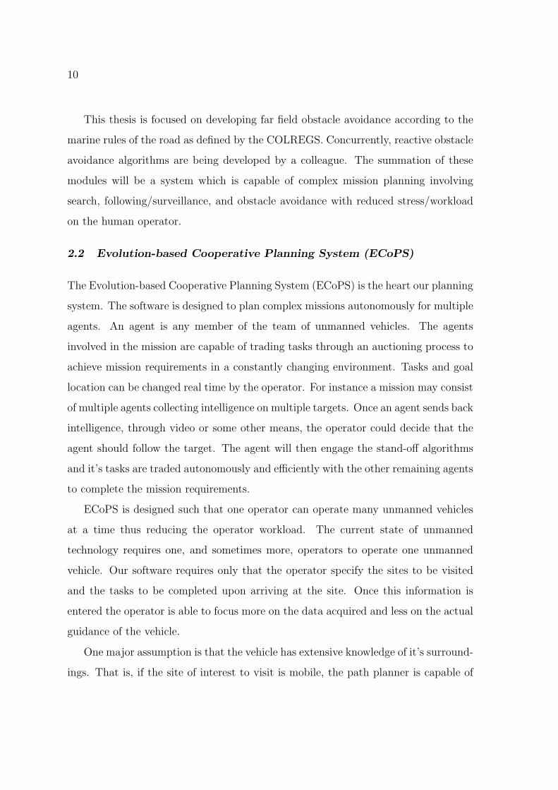
continuously evolving paths. In Figure 2.3(a), the highest utility is the average of two
distinct behaviors. ECoPS’ multi-objective approach is capable of finding the path
with the higher utility that is the average of two distinct behaviors. It is also capable
of choosing the best distinct behavior if the utility is maximized by one behavior or
the other as shown in Figure 2.3(b).
Average of two Behaviors
Behavior A Behavior B
Utility
(a) Averaging two distinct behaviors results in a
higher utility than choosing one behavior.
Average of two Behaviors
Behavior A Behavior B
Utility
(b) Averaging two distinct behaviors results in a
lower utility than choosing one behavior.
Figure 2.3: Maximizing Utility of Two Distinct Behaviors.
2.2.2 Single Vehicle Path Generation
The following is a brief description about the generation of paths for a single vehicle.
For a more detailed description see Rathbun and Capozzi [16].
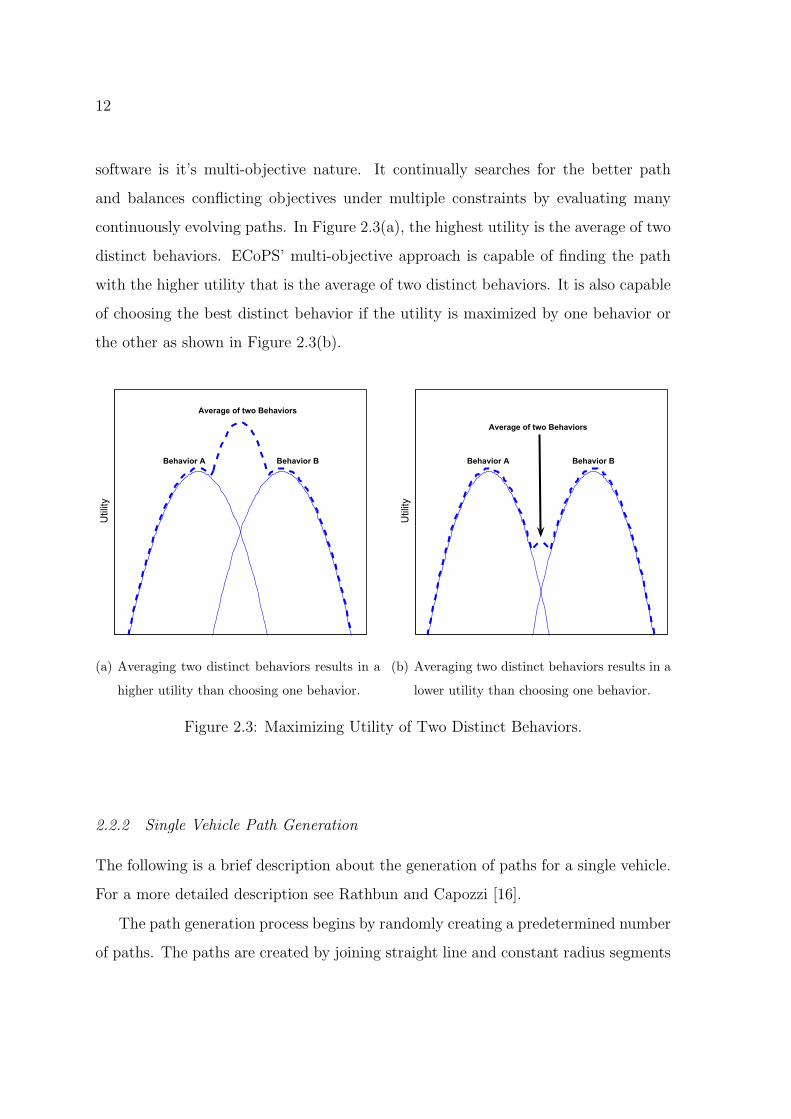
The path generation process begins by randomly creating a predetermined number
of paths. The paths are created by joining straight line and constant radius segments
13
Figure 2.4: Example of a Path connected byconstant radius curves and straight line segments.
Population
Produce
Offspring
( mutation )
Evaluate
( fitness )
Selection
Decode
Environment
Vehicle
Capabilities
Goals
Constraints
Plan Encoding BestPlan
Figure 2.5: Evolutionary Process.
together end to end as shown in Figure 2.4. Once these are created the evolution
process can begin. Figure 2.5 shows the evolutionary process. There are three basic
steps; Evaluation, Selection, and Offspring Creation (mutation).
The evolution process begins by evaluating the set of randomly generated paths
with an objective function. The objective function can vary depending on the mission
type but typically would involve things like fuel consumption, survivability, mission
accomplished (or not), timely arrival, etc. . . The general objective function is shown
in Eqn. 2.1 [17].

14
J =
NT∑i=1
(Ri(N)−Ri(sp))− C(Q(sp)) (2.1)
The first term in Eqn. 2.1 is a function of the environment states and the candidate
path, Q. It is the score gained by a candidate path during the time tsp < t ≤ tN .
The score is increased by accomplishing tasks. Ri is the score for accomplishing task
i. The vehicle score at the end of the current trajectory is Ri(sp). Ri(N) is the score
for the path from the end of the current trajectory until it’s endpoint. The difference
between Ri(N) and Ri(sp) is the score to be gained by choosing the path. C(Q(sp))
is the cost of the candidate path, Q, from the end of the committed trajectory to the
end point of the path. Costs include fuel consumption, attrition and other mission
specific parameters. The rules of the road are implemented by adding another term
into the cost function, C(Q(sp)). The added term is given by Eqn. 4.8 in Section 4.3.
Once the initial set of paths are created their cost and score is evaluated. The
objective function is used to evaluate the individual paths for their “fitness”. A higher
value means the path has better fitness. As shown in the diagram in Figure 2.5
many parameters are considered when calculating the fitness. Vehicle capabilities,
goals, constraints and environmental information are fed to the objective function to
evaluate a path score and cost. The paths are then evaluated in a tournament. The
ith candidate path competes against the other paths. For each opposing path that
the candidate path has a higher objective function result, the candidate path is given
a point. The process is repeated n times, where n is the number of paths and all
paths get their turn as the candidate path.
Moving clockwise from the evaluate box in Figure 2.5 the next step is selection.
At the end of the fitness evaluation the paths with the highest scores are selected
to be parents for the next generation of paths. For a more detail explanation of the
fitness and selection process see Pongpunwattana [18].
Now that parents have been selected, offspring must be created. These offspring

15
are created by randomly mutating the parent paths that were selected. There are five
mutation mechanisms.
1. Mutate 1-Point - This mechanism takes out a segment in the path. There are
two sections of path left over. A new segment is randomly appended to the end
of the first chunk of path and the second chunk of path is moved and connected
to the end of the newly created segment.
2. Mutate 2-Point - This mechanism cuts a chunk out of the middle of a path and
then randomly generates segments to reconnect the beginning and end of the
path.
3. Crossover - This method takes the beginning of one path and the end of another
and then connects them.
4. Mutate Shrink - Removes some random number of segments from the end of a
path.
5. Mutate Expand - Adds a random number of segments to the end of a path.
Figure 2.6 shows an example of the Mutate 1-Point mutation process. The path
on the left, path a, is the initial path. The beginning of the path is at the bottom
represented by a grey icon, the end, or goal location, is represented by the green circle
with a ‘G’. The paths are created by randomly connecting path segments together.
This does not ensure that the path connects with a desired goal location. In the path
planner there is Go To Goal functionality that connects the end of the generated path
to the desired goal location. The first step in the mutation process is to remove the
Go To Goal section of the path, shown in path b. Then in path c, a middle segment
has been removed and a new random segment inserted. Also, the chunk of path that
had been cut off is connected to the end of the new segment. Finally in path d the Go
16
Go To
Goal
Main
Path
a.) b.) c.) d.)
Figure 2.6: Example of Mutate 1-Point Mutation Process.
To Goal segments connect the mutated path back to the goal location. See Rathbun
et al.,[19] for a more detailed description of how the paths are mutated, and connected
to the goal location.
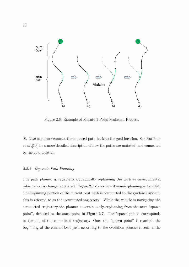
2.2.3 Dynamic Path Planning
The path planner is capable of dynamically replanning the path as environmental
information is changed/updated. Figure 2.7 shows how dynamic planning is handled.
The beginning portion of the current best path is committed to the guidance system,
this is referred to as the ‘committed trajectory’. While the vehicle is navigating the
committed trajectory the planner is continuously replanning from the next “spawn
point”, denoted as the start point in Figure 2.7. The “spawn point” corresponds
to the end of the committed trajectory. Once the “spawn point” is reached, the
beginning of the current best path according to the evolution process is sent as the

17
Start Point
Best PathNew Start
Navigate this trajectory
Start Point
Figure 2.7: Dynamic Path Planning.
new committed trajectory to the guidance system.
2.2.4 Market based protocol
The ECoPS path planner uses a market based protocol developed by Pongpunwat-
tana [18] to decrease operator workload and autonomously complete complex mis-
sions. The task trading process has no centralized planner assigning tasks. Rather
each vehicle makes it’s own trading decisions. The focus of this paper is on one vehicle
navigating according to the marine rules of the road but a complete description of
the ECoPS path planner must include a mention the task trading ability.
18
Chapter 3
INTEGRATION OF ENVIRONMENTAL INFORMATION
The ECoPS software is very flexible to changes in environmental information. We
seek to use a variety of sensors to gain as much knowledge of the environment as pos-
sible. For our initial demonstrations in a controlled environment we have integrated
a Digital Elevation Map, GPS, and RADAR data. In the future more sensors will be
added to increase the richness of the world state information.
Figure 3.1 shows the information that flows into and out of the path planner.
Some of the information such as Team Vehicles, and Team Tasks are implemented
by an operator during the initialization of the mission. These may be updated by
the operator or ECoPS, if for instance, it has reason to believe a team member is
no longer operational. Other information such as environmental and obstacle infor-
mation must be obtained from other sources. We obtain obstacle information from
a RADAR sensor, water depth information from digital nautical charts, and our ve-
hicles location from GPS. The GPS and RADAR data are obtained from sources
that use NMEA 0183 protocol. The implementation of this protocol is discussed in
Sections 3.4 and 3.5. The depth of water is obtained from a Digital Elevation Map
(DEM) and is discussed in Section 3.2.
3.1 Adaptation of ECoPS to USVs
The path planning software was originally developed for use on UAVs. The vehicle
dynamics and operating environment are quite different between UAVs and USVs.
Therefore ECoPS was modified to work with USVs.
In simulation the vehicle states are updated every time step using a simple update

19
PlanningSystemTeam Tasks:
location, uncertainty, value,
action, time
Team Vehicles:
location, fuel, capabilities
Environment:
tides, terrain
Obstacles:
location, uncertainty, effectiveness
Trajectories
Vehicle Paths
Planned
Actions
Initial Task Plans
Task Plans
Guidance
System
Planner Status & Info
Payload
Controller
Figure 3.1: Path Planning System Data Flow.
procedure. The vehicle moves with constant velocity in short straight line segments on
the path. The desired location at the end of the current time step is calculated. Then
the heading is changed to point at the desired location in the path. The command is
analogous to a rudder command that would be issued by an autopilot. Because we
do not aim to maneuver the vehicle aggressively we ignore vehicle dynamics. Rather,
the capabilities of the vehicle, such as minimum turn radius, are coded into the path
generation process. As a result we don’t worry about exceeding the limits of the
vehicle in the state update process. The vehicle position is then updated with,
Pos = v∆T (3.1)
where, v is velocity, and ∆T is the time step.
The environment and the capabilities of a USV are drastically different than a
UAV. These differences in environment and capability can be leveraged by the USV
to increase the scope of mission scenarios. For instance, a marine vehicle is capable of
coming to a complete stop, interacting with hard obstacles, and maintaining a nearly
constant position if desired. With a conventional UAV, hard obstacles are carefully
20
avoided and a forward velocity is always maintained. To take full advantage of the
USVs capability, environmental data such as depth of water, navigation aids, and
moving obstacles must be known. For the purpose of obtaining this information, the
integration of sensors using a NMEA 0183 protocol and a digital nautical chart are
discussed below.
3.2 Electronic Navigation Charts
A Digital Elevation Map (DEM) of the Puget Sound area was procured from Harvey
Greenberg at the University of Washington Department of Earth and Space Sciences.
Areas of operation could then be sampled from the DEM and the data formatted for
interpretation by ECoPS.
The data is in the Universal Transverse Mercator zone 10 (NAD27) projection.
The data forms a grid which has 30m resolution so some important features such as
buoys and shallow water boulders do not show up. The Southwest corner of the grid
is (518310, 5234460) or (47◦15’55”, 122◦45’29”) and the Northeast corner is (551220,
5289150) or (47◦45’20”, 122◦18’59”). We decided to use this section of data because it
gives a good variety of land/water features. There are islands, channels, peninsulas,
and open water.
This data does not have high enough resolution for real autonomous missions but
it is good enough to run simulations and also perform on the water testing. The
long term solution is to integrate ECoPS with Digital Navigation Charts from the
National Geospatial-Intelligence Agency (NGS). The specification is available for free
but it was a significant enough project that the integration is left for a future project.
3.3 Simulation Results using a Kinematic Model and Digital ElevationMap
Using the kinematic model and an integrated Digital Elevation map simulations were
run which show ECoPS ability to navigate through an environment with moving

21
obstacles. In this case we modeled two ferries coming to dock in downtown Seattle.
Their schedules are known and they have AIS transmitters [20] so we assume their
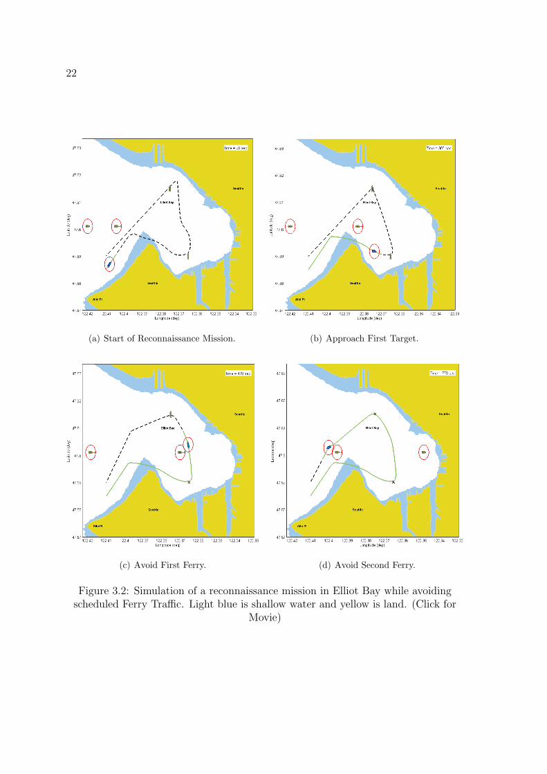
locations are known with a high level of certainty. In Figure 3.2(a) the USV is
maneuvering into Elliot Bay, WA and a ferry is also traveling into the bay cutting
near a point. In Figure 3.2(b) the USV has traveled between the point and the ferry
and is approaching the first target to be investigated. Then in Figure 3.2(c) the USV
must again avoid the ferry on it’s way to investigating the second target. This will be
a good application of the Marine Rules of the Road (to be discussed in chapter 4). It is
common courtesy to pass behind large vessels due to their low level of maneuverability.
Finally in Figure 3.2(d) the USV is returning to it’s home location but must avoid
a second ferry which is traveling through the direct path back to base. Note, in the
figure, the light blue is shallow water and the yellow represents land. The ability
to avoid land and moving boat traffic while planning efficient routes to the target
locations demonstrates ECoPS ability to handle multiple objectives simultaneously.
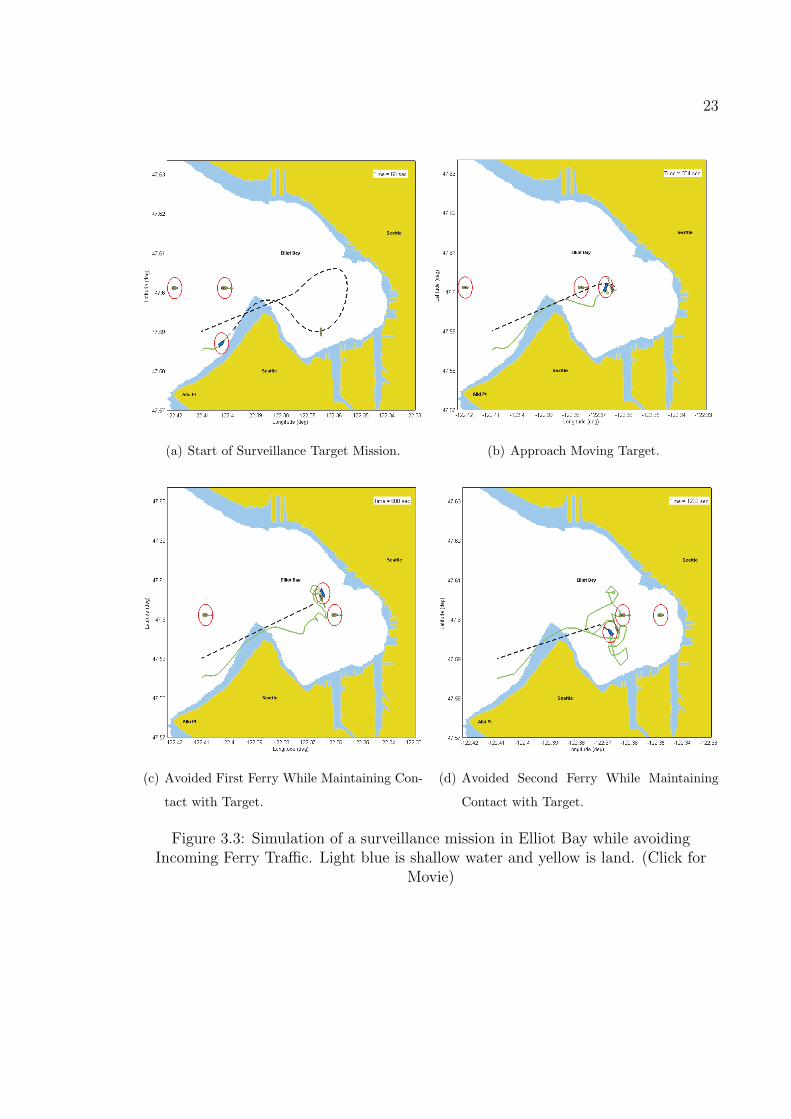
In Figure 3.3 the task is to follow and monitor a vessel in Elliot Bay. At first, in
Figure 3.3(a), the target is stationary and the path planner plans an efficient direct
route. Then in Figure 3.3(b) the target has begun to move and the path planner
is able to adapt its path to the changing position of the target. Our vessel follows
the target vessel while avoiding incoming ferry traffic in Figure 3.3(c). Then the
target changes direction and our vessel continues to follow while avoiding the second
incoming ferry, Figure 3.3(d). Again ECoPS’ multi-objective nature is demonstrated,
this time in it’s ability to follow a moving target and avoid an incoming ferry without
hitting the ferry or losing contact with the target.
3.4 Integration of GPS
Integration of GPS with ECoPS is critical for feedback of vehicle states. Our partic-
ular GPS unit is integrated with a compass and provides position, heading, course
over ground, and speed.
22
(a) Start of Reconnaissance Mission. (b) Approach First Target.
(c) Avoid First Ferry. (d) Avoid Second Ferry.
Figure 3.2: Simulation of a reconnaissance mission in Elliot Bay while avoidingscheduled Ferry Traffic. Light blue is shallow water and yellow is land. (Click for
Movie)
23
(a) Start of Surveillance Target Mission. (b) Approach Moving Target.
(c) Avoided First Ferry While Maintaining Con-
tact with Target.
(d) Avoided Second Ferry While Maintaining
Contact with Target.
Figure 3.3: Simulation of a surveillance mission in Elliot Bay while avoidingIncoming Ferry Traffic. Light blue is shallow water and yellow is land. (Click for
Movie)

24
The National Marine Electronics Association (NMEA) has specified two commu-
nication protocols for marine electronic, NMEA 2000 and NMEA 0183. NMEA 0183
is the predecessor to NMEA 2000 and was developed so that marine electronic com-
ponents from different manufacturers can communicate with each other protecting
consumers against having to use one manufacturer for all the systems on a vessel.
NMEA 2000 is a CAN-bus protocol whereas NMEA 0183 is based on ASCII se-
rial communication. Even though NMEA 2000 is newer and has greater capacity
NMEA 0183 seems to be the more commonly used communication protocol among
consumers. As such we have chosen to use NMEA 0183 devices wherever possible.
The NMEA 0183 standard is copyrighted by the National Marine Electronics
Association and at the time of this writing costs $270 [21]. An example of a NMEA
0183 sentence is shown in Figure 3.4. All NMEA 0183 sentences start with a five
character identifier preceded by a ‘$’. The ‘$’ indicates the start of a new sentence,
‘GP ’ indicates that the message is from a GPS device, ‘GLL’ says what kind of
sentence it is (there are many sentences that a GPS unit could send), in this case the
sentence is, “Geographic Position, Latitude and Longitude”. The data is deliminated
with a comma. The sentence is terminated with an asterisk followed by an optional
checksum. The checksum is the 8-bit exclusive OR of all characters in the sentence
between the ‘$’ and the ‘* ’ (including the commas). The result is converted to two
ASCII characters (0-9,A-F) and appended to the end of the sentence [22].
3.5 Integration of RADAR data
RADAR data is used to obtain information about obstacles that are not known a
priori, primarily other vessels. As with GPS, RADAR data can be obtained from a
NMEA 0183 sentence. Typically an Automatic Radar Plotting Aid (ARPA) accessory
needs to be purchased to translate the raw radar data into a NMEA sentence. The
information available from the radar is:

25
Figure 3.4: Example of a NMEA 0183 Sentence.
1. Target number
2. Target distance from own vessel
3. Bearing from own ship
4. Target speed
5. Target course
6. Distance of closest point of approach
7. Time in minutes to closest point of approach. (-) means moving away
8. Target status L/Q/T (lost from tracking/in process of acquisition/tracking)
9. Time of data in UTC format hhmmss.ss
10. Automatic or manual acquisition
A single NMEA radar sentence contains information on one target and up to ten
targets can be tracked at a time. As each sentence arrives in the path planner the

26
data is stored in a vector. The data is identified in the vector by the associated target
number.
3.6 Automatic Identification System
The Automatic Identification System provides detailed information on large vessels
which can be integrated with obstacle avoidance algorithms to define safe distances to
objects and predict future states of large vessels. It’s data is also communicated via
a NMEA 0183 sentence. The AIS system broadcasts the following useful information
every 2-10 seconds while underway and every 3 minutes while at anchor.
1. Rate and direction of turn
2. Speed over ground
3. Position accuracy
4. Longitude
5. Course over ground
6. True heading
7. Time in minutes to closest point of approach. (-) means moving away
8. Time stamp (UTC)
In addition, every 6 minutes an AIS system broadcasts the following information
which may be useful for navigation and/or target identification,
1. Radio call sign
2. Name

27
3. Type of ship/cargo
4. Dimensions of ship
5. Destination
6. Estimated time of arrival at destination (UTC)
Note, the above information is for a class A AIS system. Class B systems are
under development and nearly identical to Class A systems. Class B systems are
intended for vessels that, by the International Maritime Organization (IMO) carriage
requirements, are not necessarily required to carry AIS. The most notable difference
between the two systems is that class B does not transmit rate of turn information.
28
Chapter 4
MARINE RULES OF THE ROAD
The increased use of USVs presents new law and policy issues that have not been
addressed. Current law does not specifically address the use of unmanned vehicles in
a marine environment. The use of such vehicles presents a risk of injury and property
damage. Showalter [23] in looking at the legality of Autonomous Underwater Vehicles
found that some semi-submersible vehicles may not be considered ”vessels” at all and
therefore are not subject to current regulations. The Coast Guard says that the
vehicle must be ”...engaged in or suitable for, commerce or navigation and as a means
of transportation on water” in order to be a vessel. So autonomous vehicles used
for scientific purposes that are simply used to study and explore may, in fact, not
fit under the current definition of a ”vessel”. Her study is primarily concerned with
submerged and semi-submerged autonomous vehicles. However, it is reasonable to
think that the same semantic issues could be argued for USVs.
A natural and prudent solution is for the designer to follow the International
Collision Regulations (COLREGS) [1] until more precise law regulating USVs is en-
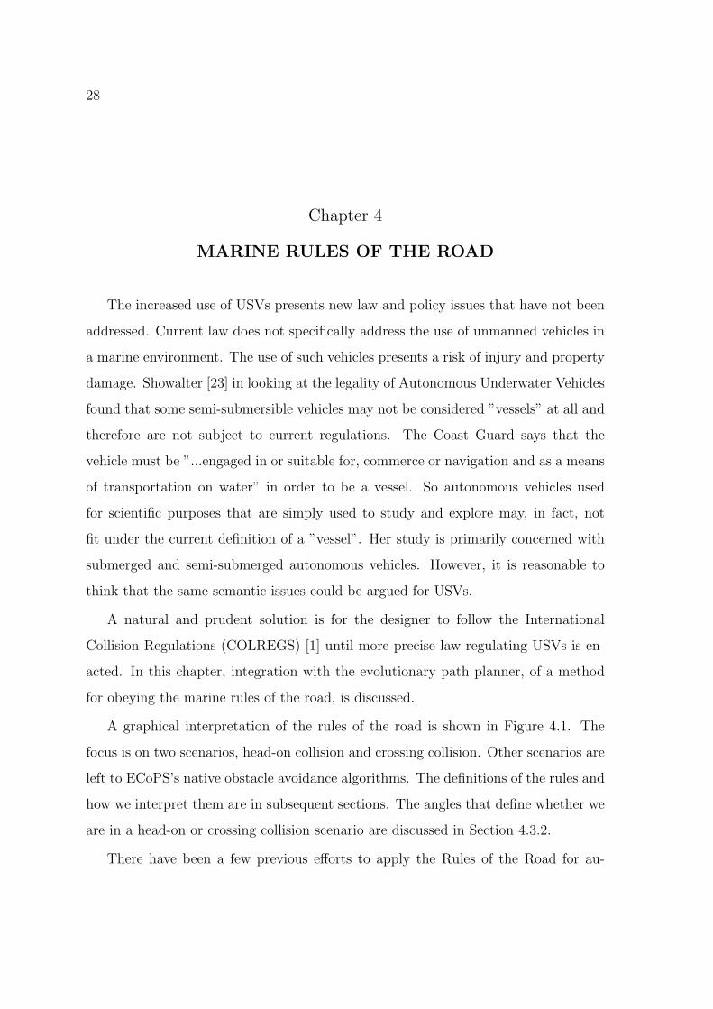
acted. In this chapter, integration with the evolutionary path planner, of a method
for obeying the marine rules of the road, is discussed.
A graphical interpretation of the rules of the road is shown in Figure 4.1. The
focus is on two scenarios, head-on collision and crossing collision. Other scenarios are
left to ECoPS’s native obstacle avoidance algorithms. The definitions of the rules and
how we interpret them are in subsequent sections. The angles that define whether we
are in a head-on or crossing collision scenario are discussed in Section 4.3.2.
There have been a few previous efforts to apply the Rules of the Road for au-
29
Crossing
Crossing
Head-OnObstacle
Head-On
120
15
o
o
Figure 4.1: Collision Scenario Definition
tonomous collision avoidance. The complexity and uncertainty of modeling marine
vehicles and their surrounding environment led Lee et al. [24], to use a fuzzy logic
approach to satisfying the COLREGS. Two groups, who have done actual testing on
the water, with vehicles of comparable size to our testbed are Benjamin et al. [25]
and Larson et al.[7]. In Benjamin et al., they use interval programming based mul-
tiobjective optimization to implement a COLREG compliant system. As discussed
in section 2.2.1, strictly following a COLREG behavior can lead to less than desir-
able results because of the complexity of the marine environment. They have chosen
to use multiobjective optimization to balance the fact that simply using a behavior
based approach can lead to suboptimal results. Larson et al. use a projected obstacle
area to develop an estimate of possible future locations of an obstacle. The choice
of vehicle action is then discretized into three possible actions based on the vehicles
location relative to the obstacle.
30
4.1 International Regulations for Avoiding Collisions at Sea
A survey of the COLREGS reveals that most of the rules concern lighting, warning
signals, application of rules, and definitions etc... and are not of concern for the
designer of path planning software. Some specific rules that require our consideration
are rule numbers:
7, 8) Rules 7 and 8 discuss identifying a possible collision and the action to take.
These are discussed in section 4.2 and 4.3.
9) Rule 9 discusses navigation through a narrow channel and is not discussed here.
14) Rule 14 defines Head-On Collision, see Section 4.1.1
15) Rule 15 defines Crossing Collision, see Section 4.1.2
16-18) Rules 16-18 determine the hierarchy of the right-of-way. It is our assumption
that our vessel will never have the right-of-way and will always be the vessel to
take action to avoid the others.
4.1.1 Head-On Collision Definition
Rule 14 states the conditions for a head-on situation,
“(a)When two power-driven vessels are meeting on reciprocal or nearly reciprocal
courses so as to involve risk of collision each shall alter her course to starboard so
that each shall pass on the port side of the other.
(b) Such a situation shall be deemed to exist when a vessel sees the other ahead
or nearly ahead and by night she could see the masthead lights of the other in a line
or nearly in a line and/or both sidelights and by day she observes the corresponding
aspect of the other vessel.”

31
A pictorial interpretation of the rule is shown in Figure 4.2. The rule is written
in such a way as to be interpreted by a human operator. This poses some issues
with trying to translate the rule to an autonomous vehicle that typically requires a
more precise definition. It was decided to use the rule shown in Eqn. 4.1. ∆θ is
shown in Eqn. 4.2 and ψ1 and ψ2 are our vehicles heading and the obstacles heading
respectively. When the condition is true we will consider our vessel to be in a head-on
configuration with another moving obstacle.
|180−∆θ| ≤ 15◦ (4.1)
∆θ = ψ1 − ψ2 (4.2)
SafetyRadius
COLREG Compliant Change of Course
(a) Complies with COLREGS.
SafetyRadius
Noncompliant Change of Course
(b) Does not Comply with COLREGS.
Figure 4.2: Example of Head-On Passing Behavior.
4.1.2 Crossing Collision Definition
Rule 15 pertains to a crossing situation. It states,
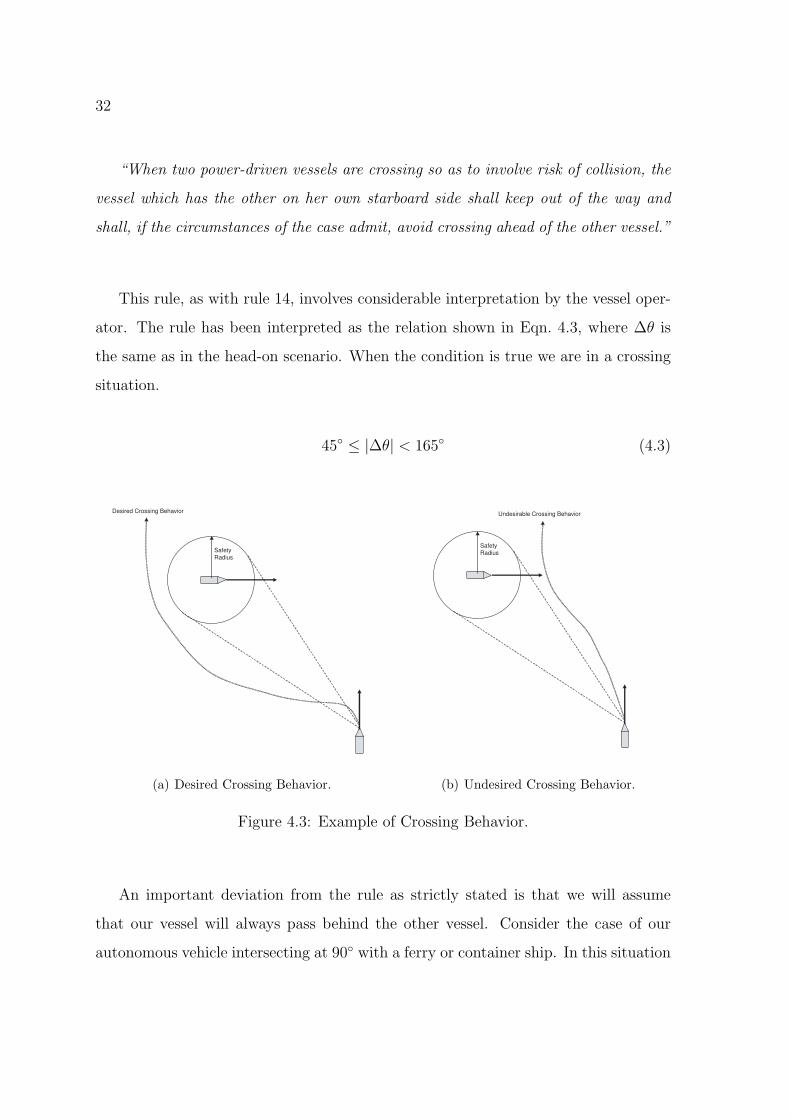
32
“When two power-driven vessels are crossing so as to involve risk of collision, the
vessel which has the other on her own starboard side shall keep out of the way and
shall, if the circumstances of the case admit, avoid crossing ahead of the other vessel.”
This rule, as with rule 14, involves considerable interpretation by the vessel oper-
ator. The rule has been interpreted as the relation shown in Eqn. 4.3, where ∆θ is
the same as in the head-on scenario. When the condition is true we are in a crossing
situation.
45◦ ≤ |∆θ| < 165◦ (4.3)
Safety
Radius
Desired Crossing Behavior
(a) Desired Crossing Behavior.
Safety
Radius
Undesirable Crossing Behavior
(b) Undesired Crossing Behavior.
Figure 4.3: Example of Crossing Behavior.
An important deviation from the rule as strictly stated is that we will assume
that our vessel will always pass behind the other vessel. Consider the case of our
autonomous vehicle intersecting at 90◦ with a ferry or container ship. In this situation
33
it is much less efficient and much more dangerous for the large vessel to change it’s
course versus our smaller highly mobile vessel. With the addition of AIS data perhaps
we could differentiate better between types of boat traffic but even with this added
information one could imagine scenarios where it’s best if we just pass behind.
4.2 Determination of Possible Collision
Deciding when to take action to follow the Rules of the Road can be difficult for
an autonomous vehicle. There is no set criteria for determining precisely when a
situation exists. As in rules 14 and 15, the determination is left to the good judgment
of the captain. The COLREGS have the following to say about determining if a risk
of collision exists:
“Every vessel shall use all available means appropriate to the prevailing circum-
stances and conditions to determine if risk of collision exists. If there is any doubt
such risk shall be deemed to exist.” - rule 7
To translate this to a more specific definition we implemented a Collision Cone
approach detailed in Chakravarthy and Ghose [26]. Their approach is inspired by
the idea that collision avoidance and achievement are basically two parts of the same
problem. That is, if you can accurately collide with something on purpose, you ought
to be able to avoid the object using related principles. At the time of publication
of their paper, robotic obstacle avoidance was a fairly new field whereas collision
achievement was a fairly mature theory in the aerospace guidance literature. Using
the ideas from aerospace literature related to collision achievement they came up the
idea of a Collision Cone.
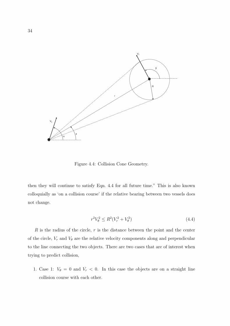
The Collision Cone is used to predict a collision between a moving point and
a moving circle. Figure 4.4 shows the geometry of a collision between a point and
a circle. It is shown in [26], that ”if a point and a circle of radius R are moving
with constant velocities such that they satisfy Eqn. 4.4 at any given instant in time,
34
R
Vθ
r
VT
φα
β
Figure 4.4: Collision Cone Geometry.
then they will continue to satisfy Eqn. 4.4 for all future time.” This is also known
colloquially as ‘on a collision course’ if the relative bearing between two vessels does
not change.
r2V 2θ ≤ R2(V 2
r + V 2θ ) (4.4)
R is the radius of the circle, r is the distance between the point and the center
of the circle, Vr and Vθ are the relative velocity components along and perpendicular
to the line connecting the two objects. There are two cases that are of interest when
trying to predict collision,
1. Case 1: Vθ = 0 and Vr < 0. In this case the objects are on a straight line
collision course with each other.

35
2. Case 2: Vθ 6= 0 and Vr < 0. In this case a collision is possible but conditions
must be found which result in a collision course.
Using the two cases above, Chakravarthy and Ghose [26], show that when Eqn. 4.5
and Eqn. 4.6 are both satisfied they are necessary and sufficient initial conditions for
a collision to occur.
r20V
2θ0 ≤ R2(V 2
r0 + V 2θ0) (4.5)
Vr0 < 0 (4.6)
Where r0 is the initial distance between the point and center of the circle, Vr0 and
Vθ0 are the initial relative velocity components along and perpendicular to the line
connecting the two objects.
4.2.1 Integration of Collision Cone with ECoPS
The Collision Cone is implemented by continuously checking conditions 4.5 and 4.6,
relative to an obstacle, for a sequence of seven points. The seven points are illustrated
in Figure 4.5. They are,
1. Current obstacle and own vehicle location.
2. Expected obstacle and own vehicle location at next spawn point.
3-7. Discretize the beginning of the base path 5 times and calculate the collision
cone at each discretization point. The length of the beginning of the path to
be discretized is equal to the length of the next committed trajectory. The
obstacles expected state at each point is used for the calculation.
The first time is based on current conditions. The second time is based on the
spawn time. The spawn location is the point at which our vehicle will commit to a
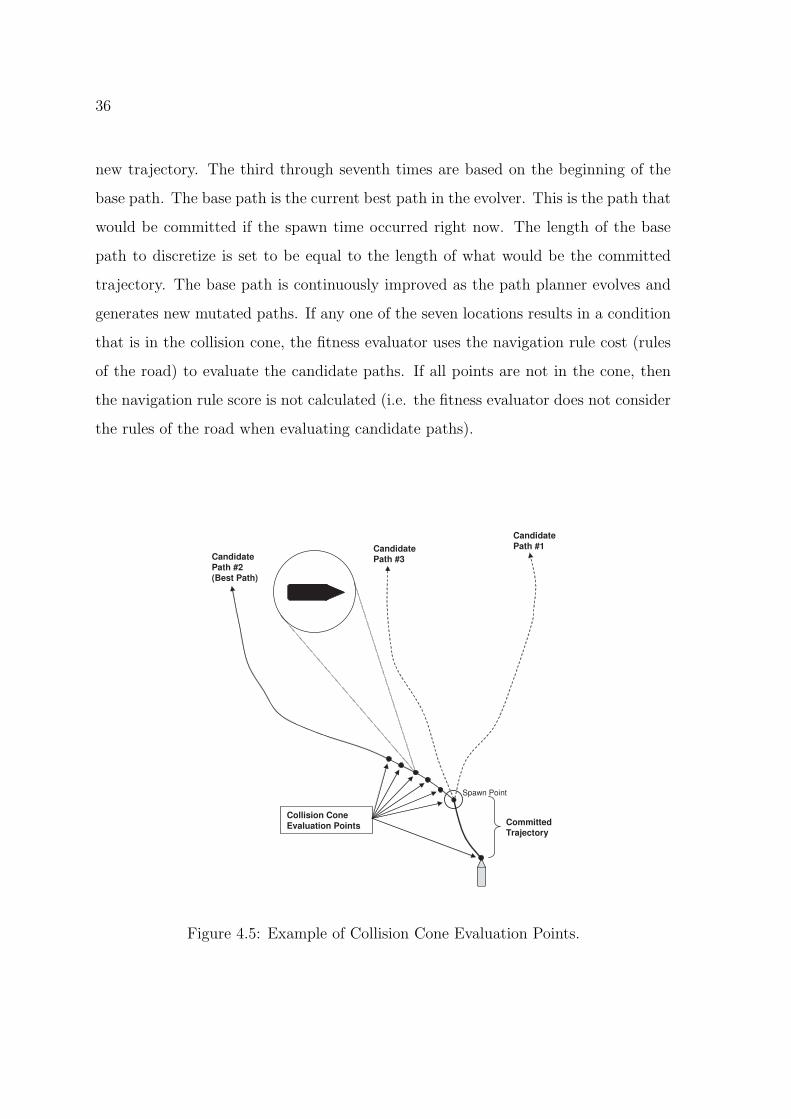
36
new trajectory. The third through seventh times are based on the beginning of the
base path. The base path is the current best path in the evolver. This is the path that
would be committed if the spawn time occurred right now. The length of the base
path to discretize is set to be equal to the length of what would be the committed
trajectory. The base path is continuously improved as the path planner evolves and
generates new mutated paths. If any one of the seven locations results in a condition
that is in the collision cone, the fitness evaluator uses the navigation rule cost (rules
of the road) to evaluate the candidate paths. If all points are not in the cone, then
the navigation rule score is not calculated (i.e. the fitness evaluator does not consider
the rules of the road when evaluating candidate paths).
Candidate
Path #1Candidate
Path #3Candidate
Path #2
(Best Path)
Committed
Trajectory
Collision Cone
Evaluation Points
Spawn Point
Figure 4.5: Example of Collision Cone Evaluation Points.
37
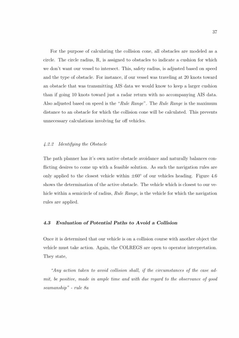
For the purpose of calculating the collision cone, all obstacles are modeled as a
circle. The circle radius, R, is assigned to obstacles to indicate a cushion for which
we don’t want our vessel to intersect. This, safety radius, is adjusted based on speed
and the type of obstacle. For instance, if our vessel was traveling at 20 knots toward
an obstacle that was transmitting AIS data we would know to keep a larger cushion
than if going 10 knots toward just a radar return with no accompanying AIS data.
Also adjusted based on speed is the “Rule Range”. The Rule Range is the maximum
distance to an obstacle for which the collision cone will be calculated. This prevents
unnecessary calculations involving far off vehicles.
4.2.2 Identifying the Obstacle
The path planner has it’s own native obstacle avoidance and naturally balances con-
flicting desires to come up with a feasible solution. As such the navigation rules are
only applied to the closest vehicle within ±60◦ of our vehicles heading. Figure 4.6
shows the determination of the active obstacle. The vehicle which is closest to our ve-
hicle within a semicircle of radius, Rule Range, is the vehicle for which the navigation
rules are applied.
4.3 Evaluation of Potential Paths to Avoid a Collision
Once it is determined that our vehicle is on a collision course with another object the
vehicle must take action. Again, the COLREGS are open to operator interpretation.
They state,
“Any action taken to avoid collision shall, if the circumstances of the case ad-
mit, be positive, made in ample time and with due regard to the observance of good
seamanship” - rule 8a

38
Active Obstacle
Inactive Obstacle
120º
Rule
Range
Figure 4.6: Active Obstacle Determination for Collision Cone Calculation.
“Any alteration of course and/or speed to avoid collision shall, if the circumstances
of the case admit, be large enough to be readily apparent to another vessel observing
visually or by radar; a succession of small alterations of course and/or speed should
be avoided” - rule 8b
These rules mean the paths that are generated by ECoPS (Section 2.2) must be
evaluated based on the rules described in Section 4.1 and also the degree to which they
take “substantial action to avoid collision”. This requirement is fulfilled by selecting
an appropriate safety radius and Rule Range.
4.3.1 Candidate Path Evaluation Process
Figure 4.7 shows a high level view of how candidate paths are evaluated. Once
our vehicle is determined to be in the Collision Cone of an object, the situation
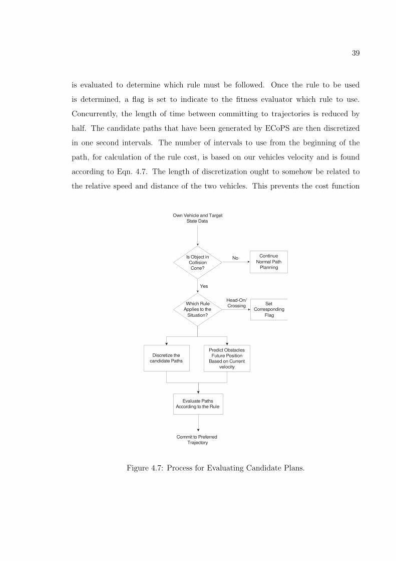
39
is evaluated to determine which rule must be followed. Once the rule to be used
is determined, a flag is set to indicate to the fitness evaluator which rule to use.
Concurrently, the length of time between committing to trajectories is reduced by
half. The candidate paths that have been generated by ECoPS are then discretized
in one second intervals. The number of intervals to use from the beginning of the
path, for calculation of the rule cost, is based on our vehicles velocity and is found
according to Eqn. 4.7. The length of discretization ought to somehow be related to
the relative speed and distance of the two vehicles. This prevents the cost function
Set
Corresponding
Flag
Own Vehicle and Target
State Data
Continue
Normal Path
Planning
No
Which Rule
Applies to the
Situation?
Yes
Head-On/
Crossing
Discretize the
candidate Paths
Predict Obstacles
Future Position
Based on Current
velocity
Is Object in
Collision
Cone?
Evaluate Paths
According to the Rule
Commit to Preferred
Trajectory
Figure 4.7: Process for Evaluating Candidate Plans.
40
from evaluating sections of the path that are far on the “other side of” the obstacle.
Rather than using relative radial velocity which could significantly change along a
committed trajectory as the orientation of the vehicles changes, we chose to base it
on our own speed. This has been shown to work well in simulation.
NumberOfDiscretizeSteps = 2 ∗ RangeToTarget
OwnV elocity(4.7)
Finally, the path is evaluated using the appropriate navigation rule. The future
state of the site is predicted by assuming it maintains constant heading and speed. It’s
position is then projected forward in time in one second intervals. At each predicted
future time step our vehicles position and heading at that time are evaluated relative
to the objects position and heading. The values are then averaged and the path with
the lowest cost is the best path for following the rules of the road. This doesn’t always
correspond to the best overall path. Things like running into land are given a higher
priority.
4.3.2 Rule Determination
Of all the rules discussed above only rules 14 and 15 need to be specifically calculated
for evaluating paths. The determination of which rule to use is made according to the
diagram shown in Figure 4.1. The diagram is a graphical interpretation of Eqns. 4.1
and 4.3. If the difference between 180◦ and the relative heading of our vehicle and the
obstacle vehicle is between 15◦ and 135◦ the situation is determined to be crossing.
If the difference between 180◦ the relative heading is between 0◦ and 15◦ then the
situation is a head-on collision. Angles between 180◦ and 135◦ are considered to
be an overtaking scenario. In an overtaking scenario the COLREGS specify that the
vehicle being overtaken should maintain it’s course and they do not specify a preferred
side for overtaking. ECoPS has algorithms that avoid collision based on the vehicles
desire to stay alive. As such we have left it to the base path planning to take care

41
of an overtaking situation. Choosing 135◦ and 15◦ as the demarcation point between
the two regimes was done somewhat arbitrarily. We chose 135◦ because the angle had
to be significantly more than 90◦ and less than 180◦. 15◦ was the value used in [25].
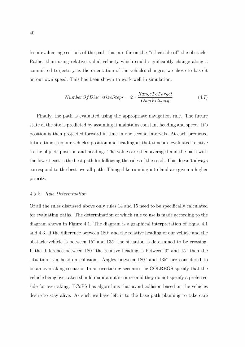
4.3.3 Head-On Rule Evaluation
The evaluation of a Head-On collision scenario is shown in Figure 4.8. In this picture
there are two candidate trajectories and the obstacle is moving directly at our initial
position. The black dots represent the end points of discretization intervals. At the
end of each interval, a vector 90◦ to the obstacle’s heading, is created pointing to the
port side of the obstacle. This vector is referred to as the Port Vector and points
to the preferred passing side. The angle between the port vector and the line from
our position to the obstacle position is calculated. The angle is denoted as αij in
Figure 4.8, where i is the Candidate Trajectory number and j is the discretization
step. The calculation of α is wrapped such that −180◦ ≤ αij ≤ 180◦.
The additional cost to implement the rules of the rules of the road in C(Q(Sp)),
from Eqn. 2.1, is determined according to Eqn. 4.8. Where n is the number of
discretation points on the candidate path as determined by Eqn. 4.7. And qij is
defined by Eqn. 4.9. A path with a lower cost is considered to comply better with
the Rules of the Road.
C(Q(Sp)) =
√∑nj=1 qij
n(4.8)
where,
qij =
0 if αij < ±90◦,
1 if αij > ±90◦.(4.9)
42
α11
α12
α22
Candidate Trajectory 1
Candidate
Trajectory 2
Figure 4.8: Evaluation of Head-On Collision Scenario.
Candidate
Trajectory 1
α11 α12
Candidate
Trajectory 2
OO
TO
Figure 4.9: Evaluation of Crossing Collision Scenario.

43
4.3.4 Crossing Rule Evaluation
Evaluation of a crossing situation is done similar to the head-on situation. A picture of
this scenario is shown in Figure 4.9. This time a Stern Vector is created. This vector
points 180◦ from the obstacles heading and again represents the preferred passing
direction. In the figure the dotted arrow represents the obstacles heading rotated by
180◦.
For both head-on and crossing scenarios we have created a vector that points to
the preferred passing side. The convienence of this design is that we can use the same
cost function for both scenarios. The only difference is in creating the passing side
vector. Therefore, Eqn. 4.8 and 4.9 are again used to calculate the cost of a potential
trajectory in the crossing collision scenario.

44
Chapter 5
SIMULATION RESULTS
Simulations were run which demonstrate the effective implementation of the rules
of the road with ECoPS. First simple simulations without terrain data were run. In
the simulations the vehicle states are initialized to encourage ECoPS to plan initial
paths that are not COLREG compliant. The paths are then evolved to comply with
the COLREGS. Both head-on and crossing scenarios are presented without terrain
data. Finally, a simulation using the digital elevation map database for Elliot Bay,
WA is shown. In this scenario there are three large vessels navigating in the Bay.
Our vessel must avoid these obstacles in a COLREG compliant manner while visiting
two targets. The results of these simulations are presented as time sequenced screen
captures from movies that were generated using data output from ECoPS.
5.1 Simulation Results without Terrain Data
Figure 5.1 shows the results of a head-on collision scenario. The obstacle is the red
icon with the arrow pointing to the right with a circle around it. The circle represents
the safety radius which we do not want our vehicle to enter, in this case the radius is
500 meters. The ‘x’ marks the goal location. The planned path is the black dashed
line and the committed trajectory is the green dashed line. In Figure 5.1(a) the initial
plan is to pass with starboard sides facing each other. To comply with the COLREGS
we must make a maneuver to our starboard such that our ports are facing each other.
At simulation time step 40 sec, Figure 5.4(b), the planned path evolves to pass on
the port side. The remaining two figures show that we indeed make it safely past the
oncoming obstacle.
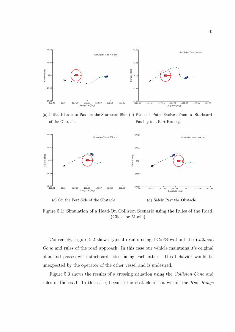
45
-122.41 -122.4 -122.39 -122.38 -122.37 -122.36 -122.3547.58
47.59
47.6
47.61
47.62
Longitude (deg)
Latit
ude
(deg
)
Simulation Time = 4 sec
(a) Initial Plan is to Pass on the Starboard Side
of the Obstacle.
-122.41 -122.4 -122.39 -122.38 -122.37 -122.36 -122.3547.58
47.59
47.6
47.61
47.62
Longitude (deg)
Latit
ude
(deg
)
Simulation Time = 4 secSimulation Time = 13 secSimulation Time = 22 secSimulation Time = 31 secSimulation Time = 40 sec
(b) Planned Path Evolves from a Starboard
Passing to a Port Passing.
-122.41 -122.4 -122.39 -122.38 -122.37 -122.36 -122.3547.58
47.59
47.6
47.61
47.62
Longitude (deg)
Latit
ude
(deg
)
Simulation Time = 4 secSimulation Time = 13 secSimulation Time = 22 secSimulation Time = 31 secSimulation Time = 40 secSimulation Time = 49 secSimulation Time = 58 secSimulation Time = 67 secSimulation Time = 76 secSimulation Time = 85 secSimulation Time = 94 secSimulation Time = 103 secSimulation Time = 112 secSimulation Time = 121 secSimulation Time = 130 sec
(c) On the Port Side of the Obstacle.
-122.41 -122.4 -122.39 -122.38 -122.37 -122.36 -122.3547.58
47.59
47.6
47.61
47.62
Longitude (deg)
Latit
ude
(deg
)
Simulation Time = 4 secSimulation Time = 13 secSimulation Time = 22 secSimulation Time = 31 secSimulation Time = 40 secSimulation Time = 49 secSimulation Time = 58 secSimulation Time = 67 secSimulation Time = 76 secSimulation Time = 85 secSimulation Time = 94 secSimulation Time = 103 secSimulation Time = 112 secSimulation Time = 121 secSimulation Time = 130 secSimulation Time = 139 secSimulation Time = 148 secSimulation Time = 157 secSimulation Time = 166 sec
(d) Safely Past the Obstacle.
Figure 5.1: Simulation of a Head-On Collision Scenario using the Rules of the Road.(Click for Movie)
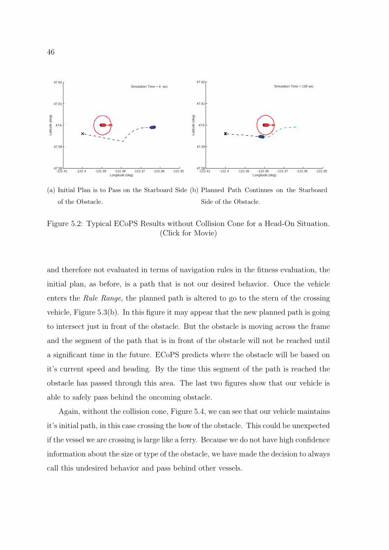
Conversely, Figure 5.2 shows typical results using ECoPS without the Collision
Cone and rules of the road approach. In this case our vehicle maintains it’s original
plan and passes with starboard sides facing each other. This behavior would be
unexpected by the operator of the other vessel and is undesired.
Figure 5.3 shows the results of a crossing situation using the Collision Cone and
rules of the road. In this case, because the obstacle is not within the Rule Range
46
-122.41 -122.4 -122.39 -122.38 -122.37 -122.36 -122.3547.58
47.59
47.6
47.61
47.62
Longitude (deg)
Latit
ude
(deg
)
Simulation Time = 4 sec
(a) Initial Plan is to Pass on the Starboard Side
of the Obstacle.
-122.41 -122.4 -122.39 -122.38 -122.37 -122.36 -122.3547.58
47.59
47.6
47.61
47.62
Longitude (deg)
Latit
ude
(deg
)
Simulation Time = 4 secSimulation Time = 13 secSimulation Time = 22 secSimulation Time = 31 secSimulation Time = 40 secSimulation Time = 49 secSimulation Time = 58 secSimulation Time = 67 secSimulation Time = 76 secSimulation Time = 85 secSimulation Time = 94 secSimulation Time = 103 secSimulation Time = 112 secSimulation Time = 121 secSimulation Time = 130 secSimulation Time = 139 sec
(b) Planned Path Continues on the Starboard
Side of the Obstacle.
Figure 5.2: Typical ECoPS Results without Collision Cone for a Head-On Situation.(Click for Movie)
and therefore not evaluated in terms of navigation rules in the fitness evaluation, the
initial plan, as before, is a path that is not our desired behavior. Once the vehicle
enters the Rule Range, the planned path is altered to go to the stern of the crossing
vehicle, Figure 5.3(b). In this figure it may appear that the new planned path is going
to intersect just in front of the obstacle. But the obstacle is moving across the frame
and the segment of the path that is in front of the obstacle will not be reached until
a significant time in the future. ECoPS predicts where the obstacle will be based on
it’s current speed and heading. By the time this segment of the path is reached the
obstacle has passed through this area. The last two figures show that our vehicle is
able to safely pass behind the oncoming obstacle.
Again, without the collision cone, Figure 5.4, we can see that our vehicle maintains
it’s initial path, in this case crossing the bow of the obstacle. This could be unexpected
if the vessel we are crossing is large like a ferry. Because we do not have high confidence
information about the size or type of the obstacle, we have made the decision to always
call this undesired behavior and pass behind other vessels.

47
-122.4 -122.39 -122.38 -122.37 -122.36 -122.35 -122.3447.58
47.59
47.6
47.61
47.62
47.63
Longitude (deg)
Latit
ude
(deg
)
Simulation Time = 4 sec
(a) Initial Plan is to Pass Across the Bow.
-122.4 -122.39 -122.38 -122.37 -122.36 -122.35 -122.3447.58
47.59
47.6
47.61
47.62
47.63
Longitude (deg)
Latit
ude
(deg
)
Simulation Time = 4 secSimulation Time = 13 secSimulation Time = 22 secSimulation Time = 31 secSimulation Time = 40 sec
(b) Planned Path Switches to Pass to the Stern.
-122.4 -122.39 -122.38 -122.37 -122.36 -122.35 -122.3447.58
47.59
47.6
47.61
47.62
47.63
Longitude (deg)
Latit
ude
(deg
)
Simulation Time = 4 secSimulation Time = 13 secSimulation Time = 22 secSimulation Time = 31 secSimulation Time = 40 secSimulation Time = 49 secSimulation Time = 58 secSimulation Time = 67 secSimulation Time = 76 secSimulation Time = 85 secSimulation Time = 94 secSimulation Time = 103 secSimulation Time = 112 secSimulation Time = 121 secSimulation Time = 130 sec
(c) At the Stern of the Obstacle.
-122.4 -122.39 -122.38 -122.37 -122.36 -122.35 -122.3447.58
47.59
47.6
47.61
47.62
47.63
Longitude (deg)
Latit
ude
(deg
)
Simulation Time = 4 secSimulation Time = 13 secSimulation Time = 22 secSimulation Time = 31 secSimulation Time = 40 secSimulation Time = 49 secSimulation Time = 58 secSimulation Time = 67 secSimulation Time = 76 secSimulation Time = 85 secSimulation Time = 94 secSimulation Time = 103 secSimulation Time = 112 secSimulation Time = 121 secSimulation Time = 130 secSimulation Time = 139 secSimulation Time = 148 secSimulation Time = 157 secSimulation Time = 166 secSimulation Time = 175 secSimulation Time = 184 secSimulation Time = 193 secSimulation Time = 202 secSimulation Time = 211 secSimulation Time = 220 secSimulation Time = 229 secSimulation Time = 238 secSimulation Time = 247 sec
(d) Safely Past the Obstacle.
Figure 5.3: Simulation of a Head-on Collision Scenario using the Rules of the Road.(Click for Movie)
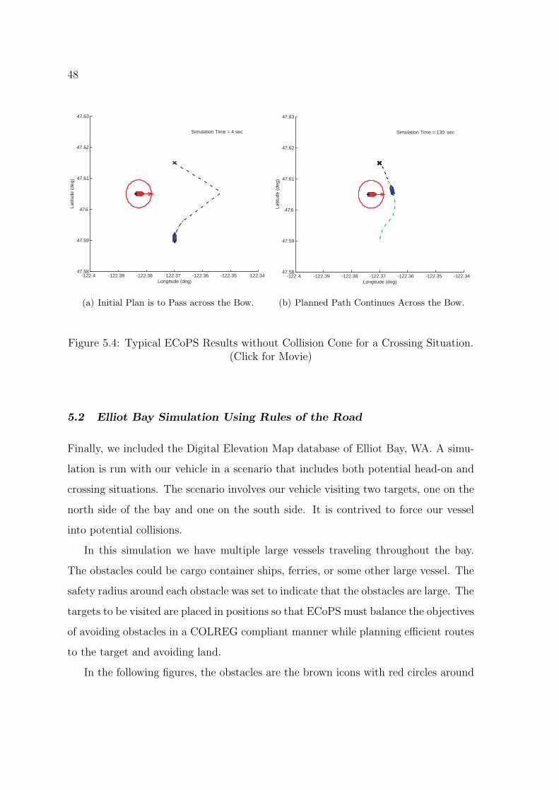
48
-122.4 -122.39 -122.38 -122.37 -122.36 -122.35 -122.3447.58
47.59
47.6
47.61
47.62
47.63
Longitude (deg)
Latit
ude
(deg
)
Simulation Time = 4 sec
(a) Initial Plan is to Pass across the Bow.
-122.4 -122.39 -122.38 -122.37 -122.36 -122.35 -122.3447.58
47.59
47.6
47.61
47.62
47.63
Longitude (deg)La
titud
e (d
eg)
Simulation Time = 4 secSimulation Time = 13 secSimulation Time = 22 secSimulation Time = 31 secSimulation Time = 40 secSimulation Time = 49 secSimulation Time = 58 secSimulation Time = 67 secSimulation Time = 76 secSimulation Time = 85 secSimulation Time = 94 secSimulation Time = 103 secSimulation Time = 112 secSimulation Time = 121 secSimulation Time = 130 sec
(b) Planned Path Continues Across the Bow.
Figure 5.4: Typical ECoPS Results without Collision Cone for a Crossing Situation.(Click for Movie)
5.2 Elliot Bay Simulation Using Rules of the Road
Finally, we included the Digital Elevation Map database of Elliot Bay, WA. A simu-
lation is run with our vehicle in a scenario that includes both potential head-on and
crossing situations. The scenario involves our vehicle visiting two targets, one on the
north side of the bay and one on the south side. It is contrived to force our vessel
into potential collisions.
In this simulation we have multiple large vessels traveling throughout the bay.
The obstacles could be cargo container ships, ferries, or some other large vessel. The
safety radius around each obstacle was set to indicate that the obstacles are large. The
targets to be visited are placed in positions so that ECoPS must balance the objectives
of avoiding obstacles in a COLREG compliant manner while planning efficient routes
to the target and avoiding land.
In the following figures, the obstacles are the brown icons with red circles around

49
them, the red circles represent a safety radius of 500m. The targets are the stationary
brown icons without red circles. Our vessel is the blue vessel with a smaller red circle.
When the target is within the red circle of radius 300m around our vehicle, we will
consider the task completed. The planned path is the black dashed line and the
committed trajectory is the solid green line.
In Figures 5.5(a) and 5.5(b) our vessel is entering Elliot Bay from the west and has
to deal with a head-on collision scenario. The path planner originally plans a path
with starboard sides facing. Once it is determined to be on a head-on collision course
with the obstacle the planned path evolves so that the vehicles pass with their ports
facing each other. Note, the initial planned path is inefficient and does not include
completion of all the tasks. The evolutionary technique is nice because it does not
require that the optimal solution is found prior to commencing a mission. As our
vessel progresses the path is continuously improved by the mutation and selection
process. When we look at the final path as shown in Figure 5.7(b) it can be seen
that the final path was efficient, completed all required tasks, and avoided other boat
traffic in compliance with the COLREGS.
After visiting the first target our vessel turns south to accomplish the second task.
As shown in Figures 5.6(a) and 5.6(b), it is faced with a potential crossing collision
with two vehicles that are traveling into the bay. At first the plan is to go across the
bow of the two vessels, then as the evolution progresses using the rules of the road
and the collision cone, the path is evolved to pass at the stern of the crossing vessels.
Finally, in Figure 5.7(a) and 5.7(b) both targets have been visited and now our
vessel must avoid a point that sticks out between our current location and our goal
location. The goal location is successfully reached
In this simulation ECoPS multi-objective nature was demonstrated in it’s ability
to plan efficient paths to accomplish multiple tasks while avoiding multiple obstacles
and land.
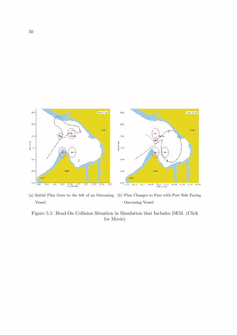
50
(a) Initial Plan Goes to the left of an Oncoming
Vessel.
(b) Plan Changes to Pass with Port Side Facing
Oncoming Vessel.
Figure 5.5: Head-On Collision Situation in Simulation that Includes DEM. (Clickfor Movie)

51
(a) Initial Plan is to go In Front of the Crossing
Vessels.
(b) Plan changes to cross behind the crossing
vessels.
Figure 5.6: Crossing Collision Situation in Simulation that Includes DEM. (Click forMovie)
(a) Plan Must Avoid Point To Get To Goal. (b) Successfully Made it to the Goal Location.
Figure 5.7: Avoiding Land on the way to the Goal Location in Simulation thatIncludes DEM. (Click for Movie)
52
Chapter 6
CONCLUSION
In recent years the science of Unmanned Aerial Vehicles (UAVs) has reached a
high level of technical maturity. Meanwhile Unmanned Surface Vehicles (USVs) have
lagged behind in technical development. The need for an improvement in USV tech-
nology to a level comparable with their airborne counterparts is clear. With recent
attacks on US marine assets and the increased use of IEDs a technically mature USV
can be used to reduce the risk to US marine assets and personnel. In addition, ben-
efits to research, surveying, border patrol, marine mammal monitoring, and many
other potential customers can also be realized.
Reducing the operator to USV ratio, requires an increase in the autonomous de-
cision making capability of USVs. In order for USVs to be accepted by the public it
must be guaranteed that the safety of people and personal property on the water is
not compromised by the addition of USVs into the field. A major hurdle to increased
autonomy is developing reliable obstacle avoidance algorithms. Obstacle avoidance
was broken down into two regimes: reactive or near-field and deliberative or far-field.
In order to achieve satisfactory performance in the face of changing and/or conflict-
ing demands an evolutionary path planning approach was used to address deliberative
obstacle avoidance. Presented here was the adaption of the evolutionary path planner
to comply with the marine rules of the road as defined by the Coast Guard Collision
Regulations (COLREGS).
This effort, coupled with previous technology developed at the AFSL and reactive
obstacle avoidance algorithms being developed by a colleague, will result in a system
which reduces operator workload by improving the autonomy of mission planning and

53
obstacle avoidance.
A small rugged Rigged Hull Inflatable boat built by Northwind Marine Inc., will
serve as the testbed for testing and verification of the obstacle avoidance algorithms.
The integration of GPS, RADAR, and Digital Elevation Map data was discussed.
This data will facilitate on the water testing testing and verification of the algorithms
to be completed in late 2007.
54
Chapter 7
FUTURE WORK
To further validate the algorithms developed here, real radar data will be used
to run simulations. Then in late 2007 field testing is planned for the path planning
system. The current digital nautical chart information is in a 30m grid, in the future
the path planner will be integrated with digital charts from the National Geospatial-
Intelligence Agency (NGS). This will improve the fidelity of environmental knowledge
by including hard obstacles such as, navigation buoys, which need to be avoided. Also,
inclusion of AIS will give us more knowledge about larger vessels and stereovision will
improve the near-field obstacle avoidance.
7.0.1 Heterogenous Teams
The Autonomous Flight Systems Lab (AFSL) at the University of Washington [13]
has many years of experience in the field of UAVs and wants to expand that expertise
to include USVs with the eventual goal of cooperative mission planning by groups
of heterogenous teams including UAVs, USVs, and Unmanned Underwater Vehicles
(UUVs).
There are practically an infinite type of missions scenarios that can be thought of to
accomplish with unmanned technology; Improvised Explosive Device (IED) detection,
Harbor Patrol, Weather Prediction, Search and Rescue, Hazardous Plum Monitoring,
Border Patrol, surveying, Forest Fire Boundary monitoring, etc...The limit seems to
be only our own imagination. Of course some of these missions lend themselves to be
best performed by one technology or another. However, many missions lend them-
selves to be best performed by a heterogeneous team of multiple vehicles cooperating
55
to use their strengths most effectively.
At the Autonomous Flight Systems Laboratory (AFSL) we hope to develop the
technology to have a fleet of heterogenous vehicles work to together to perform com-
plex missions. UUVs, developed by the Applied Physics Laboratory at the University
of Washington, have operated autonomously for 193 straight days [27]. UAVs have
been well developed and are currently used all over the world for many different
missions. A key bottleneck to achieving the goal of heterogenous teams is the cur-
rent state of USV autonomy. The ECoPS software has already been well developed
for application to UAVs and this thesis presents a step towards applying the same
techniques to USVs resulting in increased autonomy.
56
BIBLIOGRAPHY
[1] U. C. G. Commandant. International Regulations for Prevention of Collisionsat Sea, 1972 (72 COLREGS). US Coast Guard, August 1999.
[2] Moire Incorporated. Overveiw of the US Market for Unmanned Surface Vehicles(USVs), October 2003. http://www.moireinc.com/.
[3] R. Brizzolara. ONR Unmanned Sea Surface Vehicle (USSV) S & T Program. InDARPA Alignment Pathway (DAP) Combat Small Boats Industry Day, Wash-ington, D.C., August 2006. http://www.marinedd.com/DAPIndustryDaysFY06.html.
[4] J. Veers and V. Bertram. “Development of the USV Multi-Mission Surface Ve-hicle III”. In 5th International Conference on Computer Applications and Infor-mation Technology in the Maritime Industries, May 2006.
[5] U.S. Dept. of Homeland Security (DHS) and U.S. Dept. of Defense (DOD). TheNational Strategy for Maritime Security, Sept. 2005.
[6] P. Parfomak and J. Frittelli. Maritime Security: Potential Terrosist Attacks andProtection Priorities. CRS Report for Congress, Jan. 2007.
[7] J. Larson, M. Bruch, and J. Ebken. “Autonomous Navigation and ObstacleAvoidance for Unmanned Surface Vehicles”. In SPIE Unmanned Systems Tech-nology VIII, Orlando, FL, April 2006.
[8] A. Maguer, D. Gourmelon, and M. Adatte. “Flash and/or Flash-S DippingSonars on Spartan Unmanned Surface Vehicle (USV): A New Asset for LittoralWaters”. In Turkish International Conference on Acoustics, July 2005.
[9] R. Pap. Unmanned Surface Vehicle (USV). Accurate Automation Corporation.http://www.accurate-automation.com.
[10] F. Khorrami. Maritime Seaway Navigation System for Next Generation Un-manned Sea Surface Vehicles. IntelliTech Microsystems, Inc. http://www.
imicro.biz.
57
[11] International Submarine Engineering Limited. TC (Tactical Controller) kit.http://www.ise.bc.ca/TCkit.html.
[12] C. Lum, R. Rysdyk, and A. Pongpunwattana. “Autonomous Airborne Geo-magnetic Surveying and Target Identification”. In Proceedings of the 2005 In-fotech@Aerospace Conference, Arlington, VA, September 2005.
[13] Autonomous Flight Systems Laboratory. http://www.aa.washington.edu/
research/afsl/.
[14] J. Rubio, J. Vagners, and R. Rysdyk. “Adaptive Path Planning for AutonomousUAV Oceanic Search Missions”. In AIAA 1st Intelligent Systems Technical Con-ference, Chicago, IL, September 2004.
[15] R. Rysdyk. “UAV Path Following for Constant Line-of-Sight”. In 2nd AIAAUnmanned Systems Conference, San Diego, CA, September 2003.
[16] D. Rathbun and B. Capozzi. “Evolutionary Approaches to Path PlanningThrough Uncertain Environments”. In 1st AIAA Unmanned Aerospace Vehi-cles, Systems, Technologies, and Operations Conference, Portsmouth, VA, May2002.
[17] J.S. Chahl, L.C. Jain, A. Mizutani, and M. Sato-llic. Innovations in IntelligentMachines, chapter 5. Springer, 2007.
[18] A. Pongpunwattana. Real-Time Planning for Teams of Autonomous Vehiclesin Dynamic Uncertain Environments. PhD thesis, University of Washington,Seattle, WA, June 2004.
[19] D. Rathbun, S. Kragelund, A. Pongpunwattana, and B. Capozzi. “An EvolutionBased Path Planning Algorithm for Autonomous Motion of a UAV ThroughUncertain Environments”. In AIAA 21st Digital Avionics Systems Conference,Irvine, CA, October 2002. University of Washington.
[20] Washington State Ferries. Technical Specification, July 2006.
[21] National Marine Electronics Association. NMEA 0183 Standard. http://www.
nmea.org/pub/0183/.
[22] Garmin. How is the checksum calculated in NMEA 0183. http://www.garmin.com/support/faqs/faq.jsp?faq=40.

58
[23] S. Showalter. “The Legal Status of Autonomous Underwater Vehicle”. TheMarine Technology Society Journal, 38:80–83, 2004.
[24] S. Lee, K. Kwon, and J. Joh. “A Fuzzy Logic for Autonomous Navigationof Marine Vehicles Satisfying COLREG Guidelines”. International Journal ofControl, Automation and Systems, 2(2), June 2004.
[25] M. Benjamin, J. Curcio, J. Leonard, and P. Newman. “A Method for Protocol-Based Collision Avoidance between Autonomous Marine Surface Craft”. Journalof Field Robotics, 23(5), May 2006.
[26] A. Chakravarthy and D. Ghose. “Obstacle Avoidance in a Dynamic Environment:A Collision Cone Approach”. In IEEE Transactions on Systems, Man, andCybernetics - Part A: Systems and Humans, volume 28, September 1998.
[27] Applied Physics Laboratory. http://www.apl.washington.edu/projects/
seaglider/summary.html.
[28] R. Rysdyk, C. Lum, and J. Vagners. “Autonomous Orbit Coordination for TwoUnmanned Aerial Vehicles”. In Proceedings of the AIAA Guidance, Navigation,and Control Conference and Exhibit, San Francisco, CA, August 2005.
[29] U.S. Coast Guard Navigation Center. AIS Overview. http://www.navcen.uscg.gov/enav/ais/default.htm.
[30] U.S. Coast Guard Navigation Center. What AIS Broadcasts. http://www.
navcen.uscg.gov/enav/ais/what_AIS_broadcasts.htm.
Top Related