


Languages
Pages
Legal


Louisiana State UniversityLSU Digital Commons
LSU Master's Theses Graduate School
2010
Audio watermarking using transformationtechniquesRajkiran RavulaLouisiana State University and Agricultural and Mechanical College, [email protected]
Follow this and additional works at: https://digitalcommons.lsu.edu/gradschool_theses
Part of the Electrical and Computer Engineering Commons
This Thesis is brought to you for free and open access by the Graduate School at LSU Digital Commons. It has been accepted for inclusion in LSUMaster's Theses by an authorized graduate school editor of LSU Digital Commons. For more information, please contact [email protected].
Recommended CitationRavula, Rajkiran, "Audio watermarking using transformation techniques" (2010). LSU Master's Theses. 766.https://digitalcommons.lsu.edu/gradschool_theses/766

AUDIO WATERMARKING USING TRANSFORMATION
TECHNIQUES
A Thesis
Submitted to the Graduate Faculty of the
Louisiana State University and
Agricultural and Mechanical College
in partial fulfillment of the
requirements for the degree of
Master of Science in Electrical Engineering
in
The Department of Electrical and Computer Engineering
by
Rajkiran Ravula
Bachelor of Engineering in Electrical and Electronics Engineering, Osmania University, 2006
Hyderabad, India
December, 2010

ii
ACKNOWLEDGEMENTS
I would like to acknowledge following people who have encouraged, supported and
helped me complete my thesis at LSU.
I am very grateful to my advisor Dr. Suresh Rai for his guidance, patience and
understanding throughout this work. His suggestions, discussions and constant encouragement
have helped me to get a deep insight in the field of watermarking. I would like to thank Dr.
Ramachandran Vaidyanathan and Dr. Hsiao-Chun Wu for sparing their time to be a part of my
thesis advisory committee. I am very thankful to Dept. of Electrical and Computer Engineering,
Dr. James Board and Ms. Melinda Hughes for supporting me financially and making me
concentrate on my research without any other deviations.
I wish to endow my earnest gratitude to my parents, who believed in me and have been
thorough all the rough times. I also want to thank my entire family and friends for their affection,
support and compassion.
I take this opportunity to thank my friends Karunakar Reddy Gujja, Aravind, Harish
Babu, Upender, Apt#20 Tiger Plaza, Raghavendra, Naga S. Korivi and Kalyan for their help and
encouragement. I would also like to thank all my friends at LSU who made my stay here an
enjoyable and a memorable one.
iii
TABLE OF CONTENTS
Acknowledgements ....................................................................................................................... ii
List of Tables ................................................................................................................................. v
List of Figures ............................................................................................................................... vi
Abstract ....................................................................................................................................... viii
1. Introduction ........................................................................................................................... 1 1.1 Background ......................................................................................................................... 1
1.2 Steganography and Watermarking ...................................................................................... 2
1.2.1 Steganography............................................................................................................. 2
1.2.2 Watermarking ............................................................................................................. 2
1.3 Differences between Steganography and Watermarking .................................................... 4
1.4 Image and Audio Watermarking ......................................................................................... 4
1.5 Applications of Watermarking ............................................................................................ 5
1.6 Outline of the Thesis ........................................................................................................... 6
2. Audio Watermarking Techniques − Background.............................................................. 9 2.1 Features of Human Auditory System (HAS) ...................................................................... 9
2.2 Requirements of the Efficient Watermark Technique ...................................................... 10
2.3 Problems and Attacks on Audio Signals ........................................................................... 11
2.4 Audio Watermarking Techniques – A Overview ............................................................. 13
2.4.1 LSB Coding .............................................................................................................. 14
2.4.2 Spread Spectrum Technique ..................................................................................... 14
2.4.3 Patchwork Technique................................................................................................ 16
2.4.4 Quantization Index Modulation ................................................................................ 16
2.5 Conclusion ........................................................................................................................ 17
3. Transformation Techniques ............................................................................................... 18 3.1 Discrete Cosine Transform ............................................................................................... 18
3.2 Discrete Wavelet Transform (DWT) ................................................................................ 19
3.2.1 Orthogonal DWT Filters ........................................................................................... 25
3.2.2 Bi-orthogonal DWT Filters ....................................................................................... 29
3.2.3 Frame Based DWT Filters ........................................................................................ 30
3.3 Conclusion .......................................................................................................................... 32
4. Proposed Technique For Watermarking .......................................................................... 33 4.1 Encryption Techniques ..................................................................................................... 33
4.1.1 Linear Feedback Shift Register (LFSR) ................................................................... 33
4.1.2 Arnold Transform ..................................................................................................... 34
4.2 Quantization ...................................................................................................................... 34
4.3 Technique .......................................................................................................................... 36
4.3.1 Embedding Algorithm .............................................................................................. 36
4.3.1.1 Encryption ......................................................................................................... 37
iv
4.3.1.2 Wave Decomposition ........................................................................................ 38
4.3.1.3 Frames Selection ............................................................................................... 38
4.3.1.4 Embedding Watermark ..................................................................................... 38
4.3.1.5 Reconstruction .................................................................................................. 39
4.3.2 Extracting Algorithm ................................................................................................ 40
4.3.2.1 Wave Decomposition ........................................................................................ 40
4.3.2.2 Frames Selection ............................................................................................... 41
4.3.2.3 Watermark Extraction ....................................................................................... 41
4.3.2.4 Reverse Encryption ........................................................................................... 41
4.4 Discussion ......................................................................................................................... 41
5. Results and Discussion ........................................................................................................ 44 5.1 Performance Parameters ................................................................................................... 45
5.2 Experiment Setup .............................................................................................................. 46
5.3 Performance Analysis ....................................................................................................... 48
5.4 Discussion on Results ....................................................................................................... 54
6. Conclusion and Future Work ................................................................................................ 56
References .................................................................................................................................... 58
Appendix: Attack Details ........................................................................................................... 61
Vita ............................................................................................................................................... 62
v
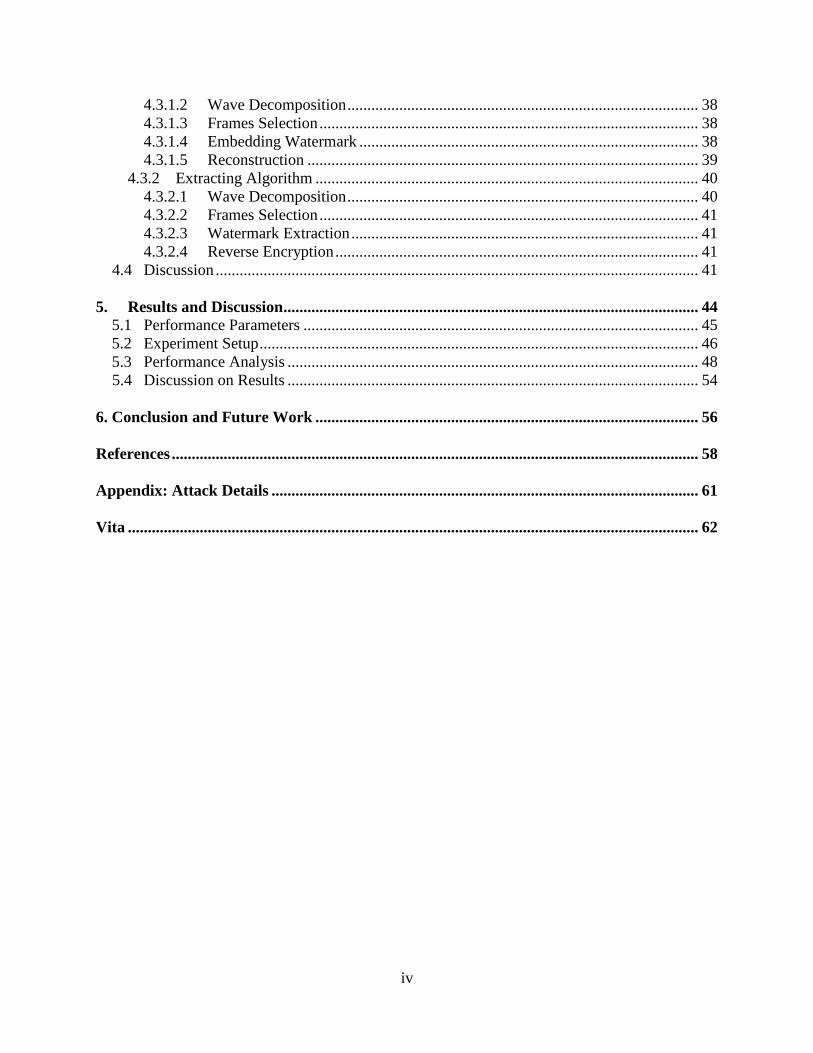
LIST OF TABLES
Table 3-1 Design concepts about orthogonal and bi-orthogonal filters ........................................ 24
Table 3-2 Daubechies wavelet filter coefficients .......................................................................... 27
Table 3-3 Low pass wavelet using approximate Hilbert transform pairs as wavelet bases [34] .. 29
Table 3-4 Coefficients of optimized DDWT filter [33] ................................................................ 31
Table 5-1 Performance evaluation of the embedded watermark with SNR of 45 dB .................. 48
Table 5-2 Performance evaluation with different algorithms ....................................................... 49
Table 5-3 Effect of encryption techniques on SNR ...................................................................... 51
Table 5-4 BER of extracted attacks with different wavelet filters for different audio signals ..... 52

vi
LIST OF FIGURES
Figure 1.1 Digital watermarking embedding .................................................................................. 3
Figure 1.2 Digital watermarking extraction .................................................................................... 4
Figure 2.1 LSB embedding ........................................................................................................... 14
Figure 2.2 Example for spread spectrum technique ..................................................................... 15
Figure 2.3 Modification of samples using QIM............................................................................ 17
Figure 3.1 Basic block view of wavelet functionality .................................................................. 21
Figure 3.2 Single level DWT analysis and synthesis blocks ........................................................ 21
Figure 3.3 3-Level DWT decomposition of signal x[n] ................................................................ 22
Figure 3.4 Wavelet decomposition coefficients of a random sinusoidal signal ........................... 23
Figure 3.5 Haar wavelet functions and filters ............................................................................... 25
Figure 3.6 db4 wavelet functions and filters ................................................................................. 28
Figure 3.7 Bi-orthogonal wavelet filter example (bior 3.5 matlab) .............................................. 30
Figure 3.8 Frame based wavelet transform ................................................................................... 31
Figure 3.9 Wavelet packet transformation .................................................................................... 32
Figure 4.1 Linear feedback shift register with polynomial (1 + x14
+ x15
) .................................... 33
Figure 4.2 Quantization of a sine wave signal .............................................................................. 35
Figure 4.3 Embedding procedure block diagram .......................................................................... 37
Figure 4.4 Reconstruction block procedure .................................................................................. 40
Figure 4.5 Extraction procedure block diagram ........................................................................... 40
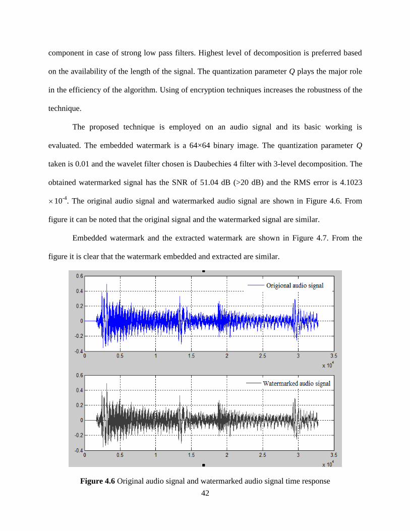
Figure 4.6 Original audio signal and watermarked audio signal time response ........................... 42
Figure 4.7 Embedded watermark and extracted watermark images ............................................. 43
Figure 5.1 Watermark (Binary image) .......................................................................................... 47
Figure 5.2 Time domain response of the considered audio signals .............................................. 47
Figure 5.3 Effect of level of the additive Gaussian Noise on the performance of the algorithm . 49
vii
Figure 5.4 Effect of level of decomposition of wavelet filter on signal to noise ratio ................. 50
Figure 5.5 Effect of quantization parameter on SNR ................................................................... 54
viii
ABSTRACT
Watermarking is a technique, which is used in protecting digital information like images,
videos and audio as it provides copyrights and ownership. Audio watermarking is more
challenging than image watermarking due to the dynamic supremacy of hearing capacity over
the visual field. This thesis attempts to solve the quantization based audio watermarking
technique based on both the Discrete Cosine Transform (DCT) and Discrete Wavelet Transform
(DWT). The underlying system involves the statistical characteristics of the signal. This study
considers different wavelet filters and quantization techniques. A comparison is performed on
diverge algorithms and audio signals to help examine the performance of the proposed method.
The embedded watermark is a binary image and different encryption techniques such as Arnold
Transform and Linear Feedback Shift Register (LFSR) are considered. The watermark is
distributed uniformly in the areas of low frequencies i.e., high energy, which increases the
robustness of the watermark. Further, spreading of watermark throughout the audio signal makes
the technique robust against desynchronized attacks. Experimental results show that the signals
generated by the proposed algorithm are inaudible and robust against signal processing
techniques such as quantization, compression and resampling. We use Matlab (version 2009b) to
implement the algorithms discussed in this thesis. Audio transformation techniques for
compression in Linux (Ubuntu 9.10) are applied on the signal to simulate the attacks such as re-
sampling, re-quantization, and mp3 compression; whereas, Matlab program for de-synchronized
attacks like jittering and cropping.
We envision that the proposed algorithm may work as a tool for securing intellectual
properties of the musicians and audio distribution companies because of its high robustness and
imperceptibility.

1
1. INTRODUCTION
Before the invention of steganography and cryptography, it was challenging to transfer
secure information and, thus, to achieve secure communication environment [1]. Some of the
techniques employed in early days are writing with an invisible ink, drawing a standard painting
with some small modifications, combining two images to create a new image, shaving the head
of the messenger in the form of a message, tattooing the message on the scalp and so on [15].
Normally an application is developed by a person or a small group of people and used by
many. Hackers are the people who tend to change the original application by modifying it or use
the same application to make profits without giving credit to the owner. It is obvious that hackers
are more in number compared to those who create. Hence, protecting an application should have
the significant priority. Protection techniques have to be efficient, robust and unique to restrict
malicious users. The development of technology has increased the scope of steganography and at
the same time decreased its efficiency since the medium is relatively insecure. This lead to the
development of the new but related technology called „Watermarking‟. Some of the applications
of watermarking include ownership protection, proof for authentication, air traffic monitoring,
medical applications etc. [1] [5] [21]. Watermarking for audio signal has greater importance
because the music industry is one of the leading businesses in the world [27].
1.1 Background
Globalization and internet are the main reasons for the growth of research and sharing of
information. However, they have become the greatest tool for malicious user to attack and pirate
the digital media. The watermarking technique during the evolution was used on images, and is
termed as Image Watermarking. Image watermarking has become popular; however, the
malicious user has started to extract the watermark creating challenges for the developers. Thus,
developers have found another digital embedding source as audio and termed such watermarking

2
as Audio Watermarking. It is very difficult to secure digital information especially the audio
and audio watermarking has become a challenge to developers because of the impact it has
created in preventing copyrights of the music [12]. Note that it is necessary to maintain the
copyright of the digital media, which is one form of intellectual property. Digital watermarking
is a technique by which copyright information is embedded into the host signal in a way that the
embedded information is imperceptible, and robust against intentional and unintentional attacks
[14].
1.2 Steganography and Watermarking
1.2.1 Steganography
Steganography is evolved from the ancient technique known as the „Cryptography‟.
Cryptography protects the contents of the message [15]. On the other hand, steganography is a
technique to send information by writing on the cover object invisibly. Steganography comes
from the Greek word that means covered writing (stego = covered and graphy = writing)
[3]. Here the authorized party is only aware of the existence of the hidden message. An ideal
steganographic technique conceals large amount of information ensuring that the modified object
is not visually or audibly distinguishable from the original object.
The steganography technique needs a cover object and message that is to be transported.
It also requires a stego key to recover the embedded message. Users having the stego key can
only access the secret message. Another important requirement for efficient steganographic
techniques is that, the cover object is modified in a way that the quality is not lost after
embedding the message.
1.2.2 Watermarking
Watermarking is a technique through which the secure information is carried without
degrading the quality of the original signal. The technique consists of two blocks:

3
(i) Embedding block
(ii) Extraction block
The system has an embedded key as in case of a steganography. The key is used to
increase security, which does not allow any unauthorized users to manipulate or extract data. The
embedded object is known as watermark, the watermark embedding medium is termed as the
original signal or cover object and the modified object is termed as embedded signal or
watermarked data [15].
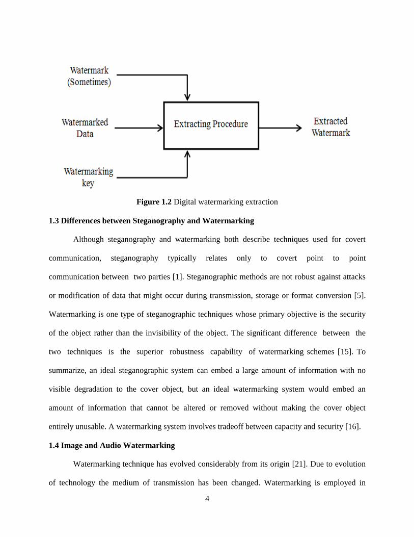
The embedding block, shown in Figure 1.1 consists of watermark, original signal (or
cover object), and watermarking key as the inputs (creates the embedded signal or watermarked
data) [15]. Whereas, the inputs for the extraction block is embedded object, key and sometimes
watermark as illustrated in Figure 1.2 [15].
The watermarking technique that does not use the watermark during extraction process is
termed as „blind watermarking.‟ Blind watermarking is superior over other watermarking
involving watermark for extraction as watermarked signal and key are sufficient to find the
embedded secret information [20].
Figure 1.1 Digital watermarking embedding
4
Figure 1.2 Digital watermarking extraction
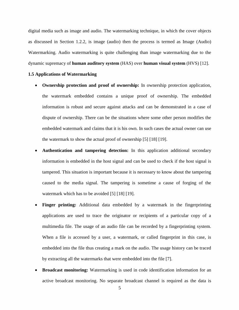
1.3 Differences between Steganography and Watermarking
Although steganography and watermarking both describe techniques used for covert
communication, steganography typically relates only to covert point to point
communication between two parties [1]. Steganographic methods are not robust against attacks
or modification of data that might occur during transmission, storage or format conversion [5].
Watermarking is one type of steganographic techniques whose primary objective is the security
of the object rather than the invisibility of the object. The significant difference between the
two techniques is the superior robustness capability of watermarking schemes [15]. To
summarize, an ideal steganographic system can embed a large amount of information with no
visible degradation to the cover object, but an ideal watermarking system would embed an
amount of information that cannot be altered or removed without making the cover object
entirely unusable. A watermarking system involves tradeoff between capacity and security [16].
1.4 Image and Audio Watermarking
Watermarking technique has evolved considerably from its origin [21]. Due to evolution
of technology the medium of transmission has been changed. Watermarking is employed in
5
digital media such as image and audio. The watermarking technique, in which the cover objects
as discussed in Section 1.2.2, is image (audio) then the process is termed as Image (Audio)
Watermarking. Audio watermarking is quite challenging than image watermarking due to the
dynamic supremacy of human auditory system (HAS) over human visual system (HVS) [12].
1.5 Applications of Watermarking
Ownership protection and proof of ownership: In ownership protection application,
the watermark embedded contains a unique proof of ownership. The embedded
information is robust and secure against attacks and can be demonstrated in a case of
dispute of ownership. There can be the situations where some other person modifies the
embedded watermark and claims that it is his own. In such cases the actual owner can use
the watermark to show the actual proof of ownership [5] [18] [19].
Authentication and tampering detection: In this application additional secondary
information is embedded in the host signal and can be used to check if the host signal is
tampered. This situation is important because it is necessary to know about the tampering
caused to the media signal. The tampering is sometime a cause of forging of the
watermark which has to be avoided [5] [18] [19].
Finger printing: Additional data embedded by a watermark in the fingerprinting
applications are used to trace the originator or recipients of a particular copy of a
multimedia file. The usage of an audio file can be recorded by a fingerprinting system.
When a file is accessed by a user, a watermark, or called fingerprint in this case, is
embedded into the file thus creating a mark on the audio. The usage history can be traced
by extracting all the watermarks that were embedded into the file [7].
Broadcast monitoring: Watermarking is used in code identification information for an
active broadcast monitoring. No separate broadcast channel is required as the data is

6
embedded in the host signal itself which is one of the main advantages of the technique
[19].
Copy control and access control: A watermark detector is usually integrated in a
recording or playback system, like in the DVD copy control algorithm [8] or during the
development of Secure Digital Music Initiative (SDMI) [7]. The copy control and access
control policy detects the watermark and it enforces the operation of particular hardware
or software in the recording set [18].
Information carrier: The blind watermarking technique can be used in this sort of
applications. These applications can transfer a lot of information and the robustness of the
algorithm is traded with the size of content [15].
Medical applications: Watermarking can be used to write the unique name of the patient
on the X-ray reports or MRI scan reports. This application is important because it is
highly advisable to have the patients name entered on reports, and reduces the
misplacements of reports which are very important during treatment [19].
Airline traffic monitoring: Watermarking is used in air traffic monitoring. The pilot
communicates with a ground monitoring system through voice at a particular frequency.
However, it can be easily trapped and attacked, and is one of the causes of miss
communication. To avoid such problems, the flight number is embedded into the voice
communication between the ground operator and the flight pilot. As the flight numbers
are unique the tracking of flights will become more secure and easy [31].
1.6 Outline of the Thesis
The central idea of this thesis is to propose a robust audio watermarking algorithm using
statistical parameters and energy of the signal in the discrete wavelet domain and also using
7
discrete cosine transform. Chapter 1 introduces the topic and provides keywords and phrases
used later in the thesis.
Chapter 2 explains the requirements of an efficient audio watermarking technique. It
provides the details of available audio watermarking techniques. Audio watermarking techniques
are employed in both time and frequency domains. From the literature it is evident that
transformation domain techniques are more robust against than time domain strategies.
Chapter 3 provides the underlying concepts of discrete cosine transform (DCT) and
discrete wavelet transform (DWT). It also explains the properties of discrete cosine transforms
with equations describing the importance of each coefficients of the DCT. The chapter also
explains different types of wavelet filters like orthogonal, bi-orthogonal, and frame based filters.
Some of the examples for each type of filters are also shown. These wavelet filters are explained
by providing the designing procedures.
Chapter 4 discusses two encryption techniques such as Arnold transformation and
Linear Feedback Shift register (LFSR). The use of encryption techniques increases the
robustness and distribution of information throughout the signal, and is important in attaining
imperceptibility property. The concept of quantization and its applications are provided using an
example. Further, Chapter 4 proposes a new audio watermarking technique involving DWT,
DCT, and the statistical parameters of the audio signal. It also integrates the HAS and DWT
properties to make the watermark robust without losing the quality of the signal. The reasons
behind the selected regions for embedding are also presented.
Chapter 5 provides the results of the technique and the performance comparison of
different algorithms with the proposed method. The performance parameters considered are bit
error rate (BER), signal to noise ratio (SNR), and normalized correlation (NC). In addition,
the effect of quantization parameter on the quality of the audio signal is also discussed. The
8
effect of the level of wavelet decomposition on the quality of the watermarked signal is also
explained. We have also presented the effect of different encryption techniques on the
performance of the watermarked signal. Performance parameters for different audio signals using
the proposed technique, their performance when undergone by different types of signal
processing attacks are evaluated. In addition, the performance of the algorithm using different
wavelet filters such as Haar, db3, db4, Hilbert-1, LeGall 5/3, and double discrete wavelet filter
(DDWT). Finally, the performance evaluation of these audio signals is compared with that
obtained from the watermarking strategies discussed in Chapter 2.
All the work presented in the thesis is done in Matlab 2009a on 2.4 GHz, 3 GB Windows
PC. To simulate the signal processing attacks like compression we have used Audio
transformation techniques compression in Ubuntu 9.10 and desynchronized attacks are done
using Matlab 2009a.
Chapter 6 concludes the thesis. It also provides the future scope of our research in the
area.
9
2. AUDIO WATERMARKING TECHNIQUES − BACKGROUND
This chapter provides the features of the human auditory system, which are important
while dealing with the audio watermarking technique. Further, this chapter considers the
requirement of an efficient watermarking strategy and different audio watermarking techniques
involving both time and frequency domain.
2.1 Features of Human Auditory System (HAS)
Note that audio watermarking is more challenging than an image watermarking technique
due to wider dynamic range of the HAS in comparison with human visual system (HVS) [12].
Human ear can perceive the power range greater than 109: 1 and range frequencies of 10
3:1 [18].
In addition, human ear can hear the low ambient Gaussian noise in the order of 70dB [18].
However, there are some useful features such as the louder sounds mask the corresponding slow
sounds. This feature can be used to embed additional information like a watermark. Further,
HAS is insensitive to a constant relative phase shift in a stationary audio signal, and, some
spectral distortions are interpreted as natural, perceptually non-annoying ones [12]. Two
properties of the HAS dominantly used in watermarking algorithms are frequency (simultaneous)
masking and temporal masking [13]:
Frequency masking: Frequency (simultaneous) masking is a frequency domain
phenomenon where low levels signal (the maskee) can be made inaudible (masked) by a
simultaneously appearing stronger signal (the masker), if the masker and maskee are
close enough to each other in frequency [13]. A masking threshold can be found and is
the level below which the audio signal is not audible. Thus, frequency domain is a good
region to check for the possible areas that have imperceptibility.
Temporal masking: In addition to frequency masking, two phenomena of the HAS in
the time domain also play an important role in human auditory perception. Those are pre-
10
masking and post-masking in time [13]. However, considering the scope of analysis in
frequency masking over temporal masking, prior is chosen for this thesis. Temporal
masking is used in application where the robustness is not of primary concentration.
2.2 Requirements of the Efficient Watermark Technique
According to IFPI (International Federation of the Phonographic Industry) [19],
audio watermarking algorithms should meet certain requirements. The most significant
requirements are perceptibility, reliability, capacity, and speed performance [9].
Perceptibility: One of the important features of the watermarking technique is that the
watermarked signal should not lose the quality of the original signal. The signal to noise
ratio (SNR) of the watermarked signal to the original signal should be maintained greater
than 20dB [19]. In addition, the technique should make the modified signal not
perceivable by human ear.
Reliability: Reliability covers the features like the robustness of the signal against the
malicious attacks and signal processing techniques. The watermark should be made in a
way that they provide high robustness against attacks. In addition, the watermark
detection rate should be high under any types of attacks in the situations of proving
ownership. Some of the other attacks summarized by Secure Digital Music Initiative
(SDMI), an online forum for digital music copyright protection, are digital-to-analog and
analog-to-digital conversions, noise addition, band-pass filtering, time-scale
modification, echo addition, and sample rate conversion [10].
Capacity: The efficient watermarking technique should be able to carry more
information but should not degrade the quality of the audio signal. It is also important to
know if the watermark is completely distributed over the host signal because, it is
11
possible that near the extraction process a part of the signal is only available. Hence,
capacity is also a primary concern in the real time situations [19].
Speed: Speed of embedding is one of the criteria for efficient watermarking technique.
The speed of embedding of watermark is important in real time applications where the
embedding is done on continuous signals such as, speech of an official or conversation
between airplane pilot and ground control staff. Some of the possible applications where
speed is a constraint are audio streaming and airline traffic monitoring. Both embedding
and extraction process need to be made as fast as possible with greater efficiency [19].
Asymmetry: If for the entire set of cover objects the watermark remains same; then,
extracting for one file will cause damage watermark of all the files. Thus, asymmetry is
also a noticeable concern. It is recommended to have unique watermarks to different files
to help make the technique more useful [19].
2.3 Problems and Attacks on Audio Signals
As discussed in Section 2.2 the important requirements of an efficient watermarking
technique are the robustness and inaudibility. There is a tradeoff between these two
requirements; however, by testing the algorithm with the signal processing attacks that gap can
be made minimal. Every application has its specific requirements, and provides an option to
choose high robustness compensating with the quality of the signal and vice-versa. Without any
transformations and attacks every watermarking technique performs efficiently. Some of the
most common types of processes an audio signal undergoes when transmitted through a medium
are as follows [11]:
Dynamics: The amplitude modification and attenuation provide the dynamics of the
attacks. Limiting, expansion and compressions are some sort of more complicated
12
applications which are the non-linear modifications. Some of these types of attacks are
re-quantization [20].
Filtering: Filtering is common practice, which is used to amplify or attenuate some part
of the signal. The basic low pass and high pass filters can be used to achieve these types
of attacks.
Ambience: In some situations the audio signal gets delayed or there are situations where
in people record signal from a source and claim that the track is theirs. Those situations
can be simulated in a room, which is of great importance to check the performance of an
audio signal.
Conversion and lossy compression: Audio generation is done at a particular sampling
frequency and bit rate; however, the created audio track will undergo so many different
types of compression and conversion techniques. Some of the most common compression
techniques are audio compression techniques based on psychoacoustic effect (MPEG and
Advanced Audio Codec (AAC)). In addition to that, it is common process that the
original audio signal will change its sampling frequencies like from 128Kbps to 64Kpbs
or 48 Kbps. There are some programs that can achieve these conversions and perform
compression operation. However, for testing purposes we have used MATLAB to
implement these applications. Attacks like re-sampling and mp3 compression provide
some typical examples.
Noise: It is common practice to notice the presence of noise in a signal when
transmitted. Hence, watermarking algorithm should make the technique robust against the
noise attacks. It is recommended to check the algorithm for this type of noise by adding
the host signal by an additive white Gaussian noise (AWGN) to check its robustness.

13
Time stretch and pitch shift: These attacks change either the length of the signal
without changing its pitch and vice versa. These are some de-synchronization attacks
which are quite common in the data transmission. Jittering is one type of such attack.
2.4 Audio Watermarking Techniques – A Overview
An audio watermarking technique can be classified into two groups based on the domain
of operation. One type is time domain technique and the other is transformation based
method. The time domain techniques include methods where the embedding is performed
without any transformation. Watermarking is employed on the original samples of the audio
signal. One of the examples of time domain watermarking technique is the least significant bit
(LSB) method. In LSB method the watermark is embedded into the least significant bits of the
host signal. As against these techniques, the transformation based watermarking methods
perform watermarking in the transformation domain. Few transformation techniques that can be
used are discrete cosine transform and discrete wavelet transform. In transformation based
approaches the embedding is done on the samples of the host signal after they are transformed.
Using of transformation based techniques provides additional information about the signal [26].
In general, the time domain techniques provide least robustness as a simple low pass
filtering can remove the watermark [20]. Hence time domain techniques are not advisable for the
applications such as copyright protection and airline traffic monitoring; however, it can be used
in applications like proving ownership and medical applications.
Watermarking techniques can be distinguished as visible or non-blind watermarking and
blind watermarking as described in Section 1.2.2. In the following, we present typical
watermarking strategies such as LSB coding, spread spectrum technique, patchwork technique,
and quantization index modulation (QIM). We provide a detailed description of transformation
methods in Chapter 3.
14
2.4.1 LSB Coding
This technique is one of the common techniques employed in signal processing
applications. It is based on the substitution of the LSB of the carrier signal with the bit pattern
from the watermark noise [21]. The robustness depends on the number of bits that are being
replaced in the host signal. This type of technique is commonly used in image watermarking
because, each pixel is represented as an integer hence it will be easy to replace the bits. The
audio signal has real values as samples, if converted to an integer will degrade the quality of the
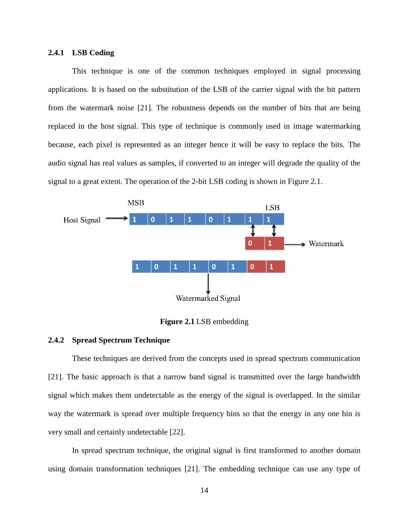
signal to a great extent. The operation of the 2-bit LSB coding is shown in Figure 2.1.
Figure 2.1 LSB embedding
2.4.2 Spread Spectrum Technique
These techniques are derived from the concepts used in spread spectrum communication
[21]. The basic approach is that a narrow band signal is transmitted over the large bandwidth
signal which makes them undetectable as the energy of the signal is overlapped. In the similar
way the watermark is spread over multiple frequency bins so that the energy in any one bin is
very small and certainly undetectable [22].
In spread spectrum technique, the original signal is first transformed to another domain
using domain transformation techniques [21]. The embedding technique can use any type of
15
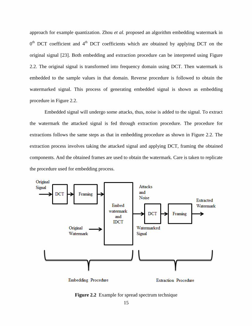
approach for example quantization. Zhou et al. proposed an algorithm embedding watermark in
0th
DCT coefficient and 4th
DCT coefficients which are obtained by applying DCT on the
original signal [23]. Both embedding and extraction procedure can be interpreted using Figure
2.2. The original signal is transformed into frequency domain using DCT. Then watermark is
embedded to the sample values in that domain. Reverse procedure is followed to obtain the
watermarked signal. This process of generating embedded signal is shown as embedding
procedure in Figure 2.2.
Embedded signal will undergo some attacks, thus, noise is added to the signal. To extract
the watermark the attacked signal is fed through extraction procedure. The procedure for
extractions follows the same steps as that in embedding procedure as shown in Figure 2.2. The
extraction process involves taking the attacked signal and applying DCT, framing the obtained
components. And the obtained frames are used to obtain the watermark. Care is taken to replicate
the procedure used for embedding process.
Figure 2.2 Example for spread spectrum technique
16
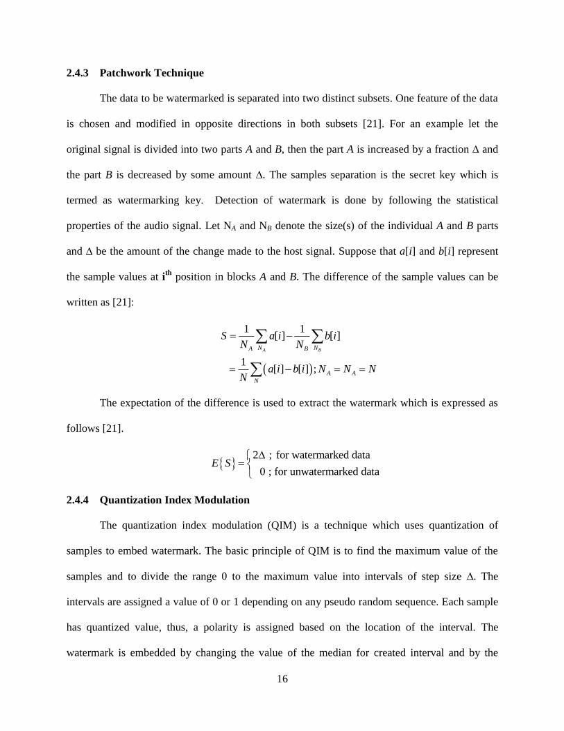
2.4.3 Patchwork Technique
The data to be watermarked is separated into two distinct subsets. One feature of the data
is chosen and modified in opposite directions in both subsets [21]. For an example let the
original signal is divided into two parts A and B, then the part A is increased by a fraction ∆ and
the part B is decreased by some amount ∆. The samples separation is the secret key which is
termed as watermarking key. Detection of watermark is done by following the statistical
properties of the audio signal. Let NA and NB denote the size(s) of the individual A and B parts
and ∆ be the amount of the change made to the host signal. Suppose that a[i] and b[i] represent
the sample values at ith
position in blocks A and B. The difference of the sample values can be
written as [21]:
1 1[ ] [ ]
1 [ ] [ ] ;
A BN NA B
A A
N
S a i b iN N
a i b i N N NN
The expectation of the difference is used to extract the watermark which is expressed as
follows [21].
2 ; for watermarked data
0 ; for unwatermarked dataE S
2.4.4 Quantization Index Modulation
The quantization index modulation (QIM) is a technique which uses quantization of
samples to embed watermark. The basic principle of QIM is to find the maximum value of the
samples and to divide the range 0 to the maximum value into intervals of step size ∆. The
intervals are assigned a value of 0 or 1 depending on any pseudo random sequence. Each sample
has quantized value, thus, a polarity is assigned based on the location of the interval. The
watermark is embedded by changing the value of the median for created interval and by the

17
similarity of the polarity and watermark bit. Suppose to embed a bit with the same polarity, the
median is moved to the same interval as shown in the right black point in the Figure 2.3 [24]. If
the watermark bit and polarity are different then the sample is moved to the median of the
nearest neighbor interval as shown in the left dark point in Figure 2.3 [24]. The quantized sample
can be expressed as shown in equation below.
Q x x
where x is the original sample value of the audio signal and Q(x) is the quantized value, hence
the quantization error is ±∆.
Figure 2.3 Modification of samples using QIM
2.5 Conclusion
In this chapter, we presented the features of human auditory system and the requirements
of the efficient watermarking techniques. Problems and possible attacks on the audio signal are
also provided. Different audio watermarking techniques in the literature such as LSB coding,
spread spectrum technique, patchwork technique, and quantization index modulation are
presented. Chapter 3 presents detailed information about the transformation techniques such as
discrete cosine transformation and discrete wavelet transformation (DWT) are provided. It also
presents different types of DWT transformations.

18
3. TRANSFORMATION TECHNIQUES
Here we discuss the background about discrete cosine transform (DCT) and discrete
wavelet transform (DWT). The chapter also presents different DWT types such as orthogonal,
bi-orthogonal and frame based filters.
3.1 Discrete Cosine Transform
The discrete cosine transform is a technique for converting a signal into elementary
frequency components [25]. The DCT can be employed on both one-dimensional and two-
dimensional signals like audio and image, respectively. The discrete cosine transform is the
spectral transformation, which has the properties of Discrete Fourier Transformation [25]. DCT
uses only cosine functions of various wave numbers as basis functions and operates on real-
valued signals and spectral coefficients. DCT of a 1-dimensional (1-d) sequence and the
reconstruction of original signal from its DCT coefficients termed as inverse discrete cosine
transform (IDCT) can be computed using equations [25]. In the following, ( )dctf x is original
sequence while ( )dctC u denotes the DCT coefficients of the sequence.
1
1
1
1
1 1
1
1
1 1
2 1cos , 0,1,2,..., -1
2
2 1cos , 0,1,2,..., -1
2
t
t
N
dct dct t
x t
N
dct dct t
u t
x uC u u f x for u N
N
x uf x u C u for x N
N
1
1
1 0
( )2
0
t
t
for uN
where u
for uN
From the equation for ( )dctC u it can be inferred that for u = 0, the component is the
average of the signal also termed as dc coefficient in literature [28]. And all the other

19
transformation coefficients are called as ac coefficients. Some of the important applications of
DCT are image compression and signal compression.
The most useful applications of two-dimensional (2-d) DCT are the image compression
and encryption [25]. The 1-d DCT equations, discussed above, can be used to find the 2-d DCT
by considering every row as an individual 1-d signal. Thus, DCT coefficients of an M×N two-
dimensional signals 2 ( , )dctC u v and their reconstruction 2 ( , )dctf x y can be calculated by the
equations below.
2 2
2 2
1 1
2 2
0 0 2 2
1 1
2 2
0 0 2 2
2
2 1 2 1, , cos cos
2 2
2 1 2 1, , cos cos
2 2
where & 0,1,2,...., -1 an
t t
t t
M N
dct dct
x y t t
M N
dct dct
u v t t
t
x u y vC u v u v f x y
M N
x u y vf x y u v C u v
M N
u x M
2
2 2
2 2
d & 0,1,2,....., -1
1 1 0 0
& 2 2
0 0
t
t t
t t
v y N
for u for vN N
u v
for u for vN N
Some of the properties of DCT are de-correlation, energy compaction, separability,
symmetry and orthogonality [12]. DCT provides interpixel redundancy for most of natural
images and coding efficiency is maintained while encoding the uncorrelated transformation
coefficients [28]. DCT packs the energy of the signal into the low frequency regions which
provides an option of reducing the size of the signal without degrading the quality of the signal.
3.2 Discrete Wavelet Transform (DWT)
Majority of the signals in practice are represented in time domain. Time-amplitude
representation is obtained by plotting the time domain signal. However, the analysis of the signal
20
in time domain cannot give complete information of the signal since it cannot provide the
different frequencies available in the signal [26].
Frequency domain provides the details of the frequency components in the signal which
are importance in some applications like electrocardiography (ECG), graphical recording of
heart's electrical activity or electroencephalography (EEG), an analysis of electrical activity of
human brain [26].The frequency spectrum of a signal is basically the frequency components
(spectral components) of that signal [26]. The main drawback of frequency domain is it does not
provide when in time these frequencies exist.
There are considerable drawbacks in either time domain or frequency domains, which are
rectified in wavelet transform. Wavelet Transform provides the time-frequency representation of
the signal. Some of the other types of time-frequency representation are short time Fourier
transformation, Wigner distributions, etc. There are different types of wavelet transforms such as
continuous wavelet transform (CWT) and discrete wavelet transform (DWT). CWT provides
great redundancy of reconstruction of the signal whereas DWT provides the sufficient
information for both analysis and synthesis signal and is easier to implement as compared to
CWT [26].
A complete structure of wavelet contains domain processing analysis block and a
synthesis block. Analysis or decomposition block decomposes the signal into wavelet
coefficients. The reconstruction process is the inverse of decomposition process. Here, the block
takes the decomposed signal and synthesizes (near) original signal. A view of the wavelet
process is shown in Figure 3.1. From the figure the original signal is decomposed in the analysis
block and the signal is reconstructed using the synthesis block. Filters used in the analysis and
synthesis block

21
Figure 3.1 Basic block view of wavelet functionality
The operation of 1-level discrete wavelet transform decomposition is to separate high
pass and low pass components. Thus, process involves passing the time-domain signal x[n]
through a high pass filter g0[n] and down sampling the signal obtained yields detailed
coefficients (D). And, passing x[n] through low pass filters h0 [n]and down sampling generated
approximate coefficients (A). The working principle is shown in Figure 3.2.
Figure 3.2 Single level DWT analysis and synthesis blocks
22
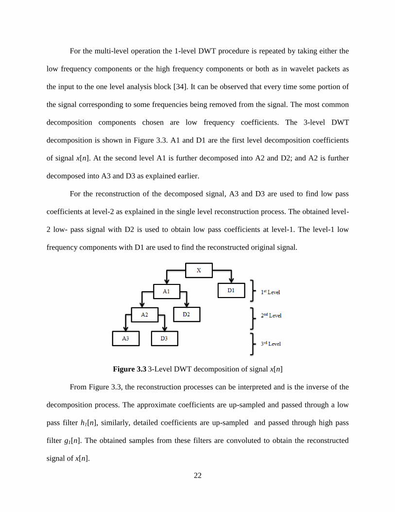
For the multi-level operation the 1-level DWT procedure is repeated by taking either the
low frequency components or the high frequency components or both as in wavelet packets as
the input to the one level analysis block [34]. It can be observed that every time some portion of
the signal corresponding to some frequencies being removed from the signal. The most common
decomposition components chosen are low frequency coefficients. The 3-level DWT
decomposition is shown in Figure 3.3. A1 and D1 are the first level decomposition coefficients
of signal x[n]. At the second level A1 is further decomposed into A2 and D2; and A2 is further
decomposed into A3 and D3 as explained earlier.
For the reconstruction of the decomposed signal, A3 and D3 are used to find low pass
coefficients at level-2 as explained in the single level reconstruction process. The obtained level-
2 low- pass signal with D2 is used to obtain low pass coefficients at level-1. The level-1 low
frequency components with D1 are used to find the reconstructed original signal.
Figure 3.3 3-Level DWT decomposition of signal x[n]
From Figure 3.3, the reconstruction processes can be interpreted and is the inverse of the
decomposition process. The approximate coefficients are up-sampled and passed through a low
pass filter h1[n], similarly, detailed coefficients are up-sampled and passed through high pass
filter g1[n]. The obtained samples from these filters are convoluted to obtain the reconstructed
signal of x[n].
23
From Figure 3.3 it is clear that the original signal can be reconstructed by combining the
highest level available decomposed coefficients. In other words x[n] can be reconstructed using
high and low pass filters g1[n] and h1[n], respectively. Figure 3.2 illustrates this operation.
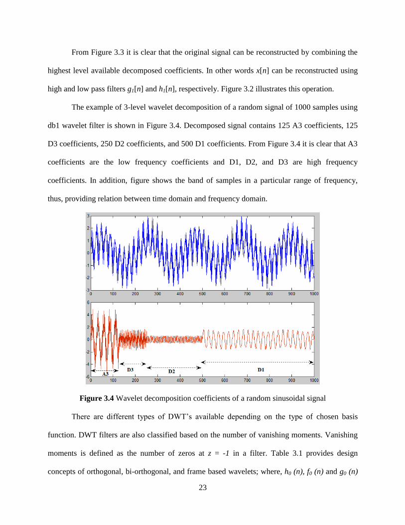
The example of 3-level wavelet decomposition of a random signal of 1000 samples using
db1 wavelet filter is shown in Figure 3.4. Decomposed signal contains 125 A3 coefficients, 125
D3 coefficients, 250 D2 coefficients, and 500 D1 coefficients. From Figure 3.4 it is clear that A3
coefficients are the low frequency coefficients and D1, D2, and D3 are high frequency
coefficients. In addition, figure shows the band of samples in a particular range of frequency,
thus, providing relation between time domain and frequency domain.
Figure 3.4 Wavelet decomposition coefficients of a random sinusoidal signal
There are different types of DWT‟s available depending on the type of chosen basis
function. DWT filters are also classified based on the number of vanishing moments. Vanishing
moments is defined as the number of zeros at z = -1 in a filter. Table 3.1 provides design
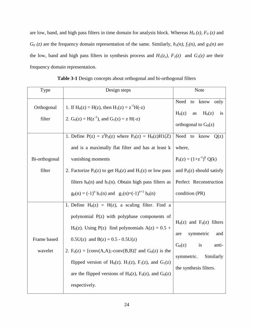
concepts of orthogonal, bi-orthogonal, and frame based wavelets; where, h0 (n), f0 (n) and g0 (n)
24
are low, band, and high pass filters in time domain for analysis block. Whereas H0 (z), F0 (z) and
G0 (z) are the frequency domain representation of the same. Similarly, h1(n), f1(n), and g1(n) are
the low, band and high pass filters in synthesis process and H1(z,), F1(z) and G1(z) are their
frequency domain representation.
Table 3-1 Design concepts about orthogonal and bi-orthogonal filters
Type Design steps Note
Orthogonal
filter
1. If H0(z) = H(z), then H1(z) = z-1
H(-z)
2. G0(z) = H(z-1
), and G1(z) = z H(-z)
Need to know only
H0(z) as H0(z) is
orthogonal to G0(z)
Bi-orthogonal
filter
1. Define P(z) = zlP0(z) where P0(z) = H0(z)H1(Z)
and is a maximally flat filter and has at least k
vanishing moments
2. Factorize P0(z) to get H0(z) and H1(z) or low pass
filters h0(n) and h1(n). Obtain high pass filters as
g0(n) = (-1)n h1(n) and g1(n)=(-1)
n+1 h0(n)
Need to know Q(z)
where,
P0(z) = (1+z-1
)k Q(k)
and P0(z) should satisfy
Perfect Reconstruction
condition (PR)
Frame based
wavelet
1. Define H0(z) = H(z), a scaling filter. Find a
polynomial P(z) with polyphase components of
H0(z). Using P(z) find polynomials A(z) = 0.5 +
0.5U(z) and B(z) = 0.5 - 0.5U(z)
2. F0(z) = [conv(A,A);-conv(B,B)]' and G0(z) is the
flipped version of H0(z). H1(z), F1(z), and G1(z)
are the flipped versions of H0(z), F0(z), and G0(z)
respectively.
H0(z) and F0(z) filters
are symmetric and
G0(z) is anti-
symmetric. Similarly
the synthesis filters.
25
3.2.1 Orthogonal DWT Filters
The analysis and synthesis filter design procedure for orthogonal DWT wavelets are
provided in Table 3.1. Note that the functions for decomposition and reconstruction are the same.
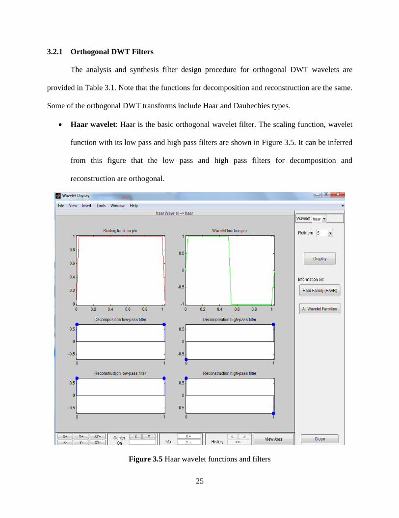
Some of the orthogonal DWT transforms include Haar and Daubechies types.
Haar wavelet: Haar is the basic orthogonal wavelet filter. The scaling function, wavelet
function with its low pass and high pass filters are shown in Figure 3.5. It can be inferred
from this figure that the low pass and high pass filters for decomposition and
reconstruction are orthogonal.
Figure 3.5 Haar wavelet functions and filters
26
The mathematical functions for wavelet and scaling functions are given below
1 0 1,
0
for tt
otherwise
11 0 ,
2
11 1,
2
0
for t
t for t
otherwise
The significant property of Haar Wavelet is any real function can be
approximated. In addition to that, the implementation is easy as there are two components
in the filter design and require less precision. The vanishing moments for Haar wavelet is
1 and is the basic wavelet. Haar wavelet is extensively used in image compression
applications due to its simple wavelet and scaling functions.
Daubechies wavelet: Daubechies wavelets define a family of orthogonal wavelet and are
characterized by more than single number of vanishing moments. Matlab provides such
wavelet characteristics as db2, db3, db4, db6, db8, etc. The vanishing moments for db2 is
1 which is same as Haar wavelet. In general, dbN wavelet contains N/2 vanishing
moments.
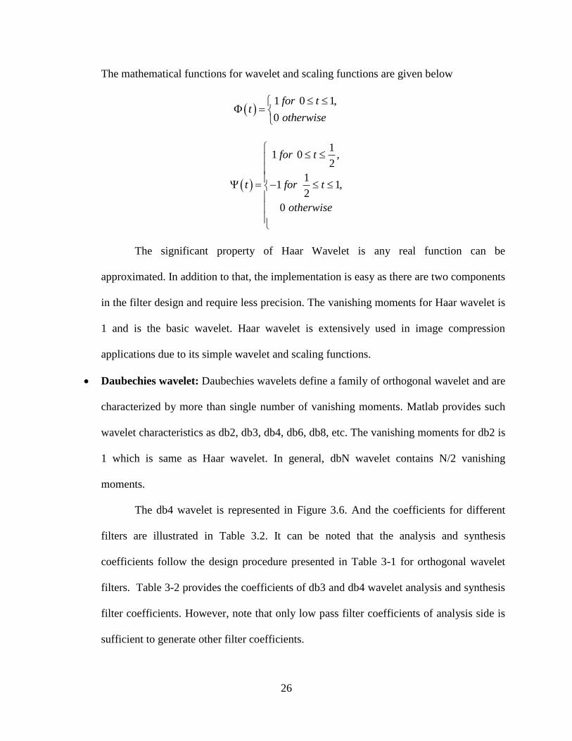
The db4 wavelet is represented in Figure 3.6. And the coefficients for different
filters are illustrated in Table 3.2. It can be noted that the analysis and synthesis
coefficients follow the design procedure presented in Table 3-1 for orthogonal wavelet
filters. Table 3-2 provides the coefficients of db3 and db4 wavelet analysis and synthesis
filter coefficients. However, note that only low pass filter coefficients of analysis side is
sufficient to generate other filter coefficients.
27
Table 3-2 Daubechies wavelet filter coefficients
Filter
Low pass filter coefficients High pass filter coefficients
Analysis (h0) Synthesis(g0) Analysis (h1) Synthesis (g1)
db3
0.0352262919
-0.0854412739
-0.1350110200
0.4598775021
0.8068915093
0.3326705530
-0.3326705530
0.8068915093
-0.4598775021
-0.1350110200
0.0854412739
0.0352262919
0.3326705530
0.8068915093
0.4598775021
-0.1350110200
-0.0854412739
0.0352262919
0.0352262919
0.0854412739
-0.1350110200
-0.4598775021
0.8068915093
-0.3326705530
db4
-0.0105974018
0.0328830117
0.0308413818
-0.1870348117
-0.0279837694
0.6308807679
0.7148465706
0.2303778133
-0.2303778133
0.7148465706
-0.6308807679
-0.0279837694
0.1870348117
0.0308413818
-0.0328830117
-0.0105974018
0.2303778133
0.7148465706
0.6308807679
-0.0279837694
-0.1870348117
0.0308413818
0.0328830117
-0.0105974018
-0.0105974018
-0.0328830117
0.0308413818
0.1870348117
-0.0279837694
-0.6308807679
0.7148465706
-0.2303778133
The coefficients are generated using following Matlab code:
[LO_A, HI_A, LO_S, HI_S] = wfilters('Wavelet type');
Where LO_A, HI_A, LO_S, and HI_S are analysis low pass, analysis high pass, synthesis
low pass, and synthesis high pass filter coefficients respectively. „Wavelet type‟ is chosen based
on the type of wavelet filters. For example, to find filter coefficients of db3 wavelet replace
„Wavelet type‟ with „db3‟.
28
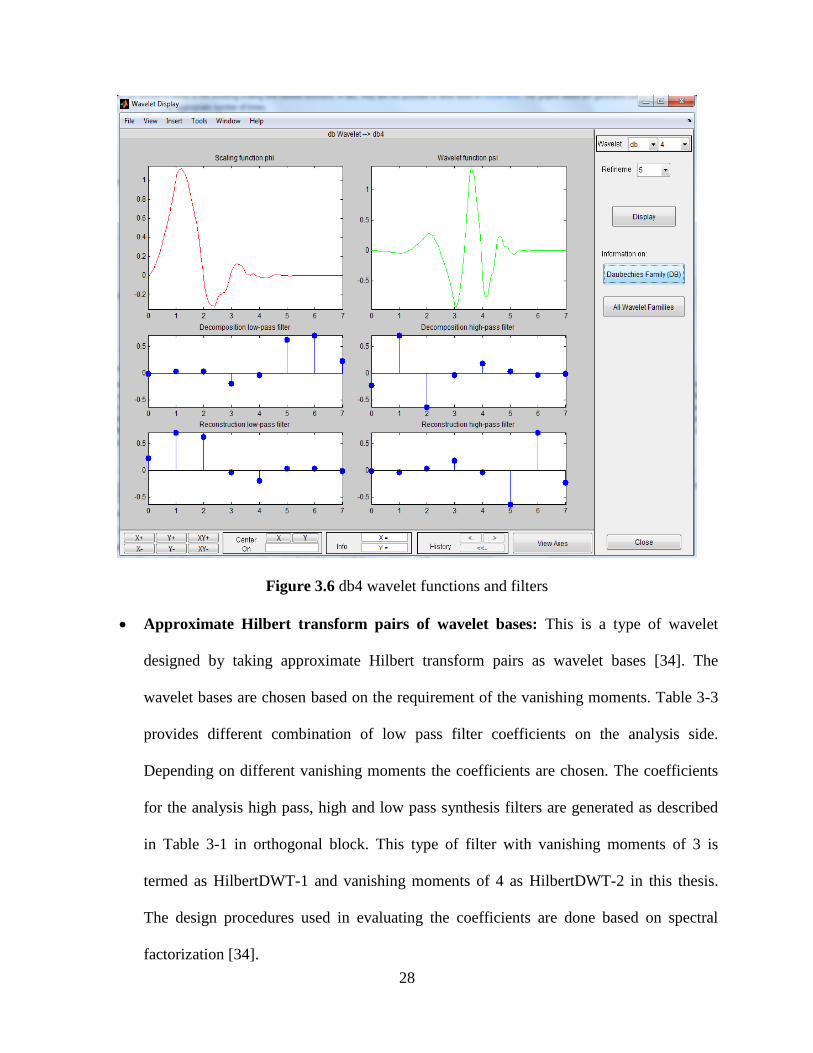
Figure 3.6 db4 wavelet functions and filters
Approximate Hilbert transform pairs of wavelet bases: This is a type of wavelet
designed by taking approximate Hilbert transform pairs as wavelet bases [34]. The
wavelet bases are chosen based on the requirement of the vanishing moments. Table 3-3
provides different combination of low pass filter coefficients on the analysis side.
Depending on different vanishing moments the coefficients are chosen. The coefficients
for the analysis high pass, high and low pass synthesis filters are generated as described
in Table 3-1 in orthogonal block. This type of filter with vanishing moments of 3 is
termed as HilbertDWT-1 and vanishing moments of 4 as HilbertDWT-2 in this thesis.
The design procedures used in evaluating the coefficients are done based on spectral
factorization [34].
29
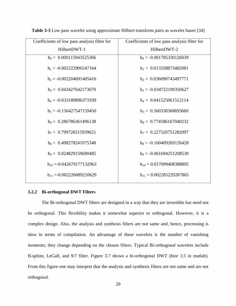
Table 3-3 Low pass wavelet using approximate Hilbert transform pairs as wavelet bases [34]
Coefficients of low pass analysis filter for
HilbertDWT-1
Coefficients of low pass analysis filter for
HilbertDWT-2
h0 = 0.000115943525366
h1 = -0.002222900247164
h2 = -0.002204691405416
h3 = 0.043427642173670
h4 = -0.033189896371939
h5 = -0.156427547159450
h6 = 0.286786361496138
h7 = 0.799726515939621
h8 = 0.498278241075348
h9 = 0.024829159690485
h10 =-0.042679177132963
h11 =-0.002226089210629
h0 = -0.001785330126039
h1 = 0.013358873482081
h2 = 0.036090743497771
h3 = -0.034722190350627
h4 = 0.041525061512114
h5 = 0.560358368693660
h6 = 0.774586167040232
h7 = 0.227520751282097
h8 = -0.160409269126428
h9 = -0.061694251208530
h10 = 0.017099408388895
h11 = 0.002285229287865
3.2.2 Bi-orthogonal DWT Filters
The Bi-orthogonal DWT filters are designed in a way that they are invertible but need not
be orthogonal. This flexibility makes it somewhat superior to orthogonal. However, it is a
complex design. Also, the analysis and synthesis filters are not same and, hence, processing is
slow in terms of compilation. An advantage of these wavelets is the number of vanishing
moments; they change depending on the chosen filters. Typical Bi-orthogonal wavelets include
B-spline, LeGall, and 9/7 filter. Figure 3.7 shows a bi-orthogonal DWT (bior 3.5 in matlab).
From this figure one may interpret that the analysis and synthesis filters are not same and are not
orthogonal.

30
Figure 3.7 Bi-orthogonal wavelet filter example (bior 3.5 matlab)
3.2.3 Frame Based DWT Filters
The wavelet decomposition can also be done using packets and frames. The frame
decomposition using wavelets are shown Figure 3.8. The original signal is divided into three
frames rather than two in earlier cases. The three splitting functions are low pass h0[n]; band pass
f0[n], and high pass g0[n]. The higher level decomposition is done taking low frequency
components as the parent signal.
We have chosen „frames‟ for our study in this thesis. Let A (B) be a matrix that analyzes
(synthesizes) the signal x[n]. If A and B are rectangular matrices and B is pseudo-inverse of A,
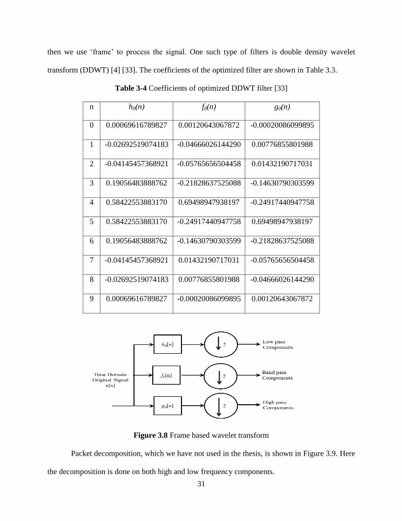
31
then we use „frame‟ to process the signal. One such type of filters is double density wavelet
transform (DDWT) [4] [33]. The coefficients of the optimized filter are shown in Table 3.3.
Table 3-4 Coefficients of optimized DDWT filter [33]
n h0(n) f0(n) g0(n)
0 0.00069616789827 0.00120643067872 -0.00020086099895
1 -0.02692519074183 -0.04666026144290 0.00776855801988
2 -0.04145457368921 -0.05765656504458 0.01432190717031
3 0.19056483888762 -0.21828637525088 -0.14630790303599
4 0.58422553883170 0.69498947938197 -0.24917440947758
5 0.58422553883170 -0.24917440947758 0.69498947938197
6 0.19056483888762 -0.14630790303599 -0.21828637525088
7 -0.04145457368921 0.01432190717031 -0.05765656504458
8 -0.02692519074183 0.00776855801988 -0.04666026144290
9 0.00069616789827 -0.00020086099895 0.00120643067872
Figure 3.8 Frame based wavelet transform
Packet decomposition, which we have not used in the thesis, is shown in Figure 3.9. Here
the decomposition is done on both high and low frequency components.
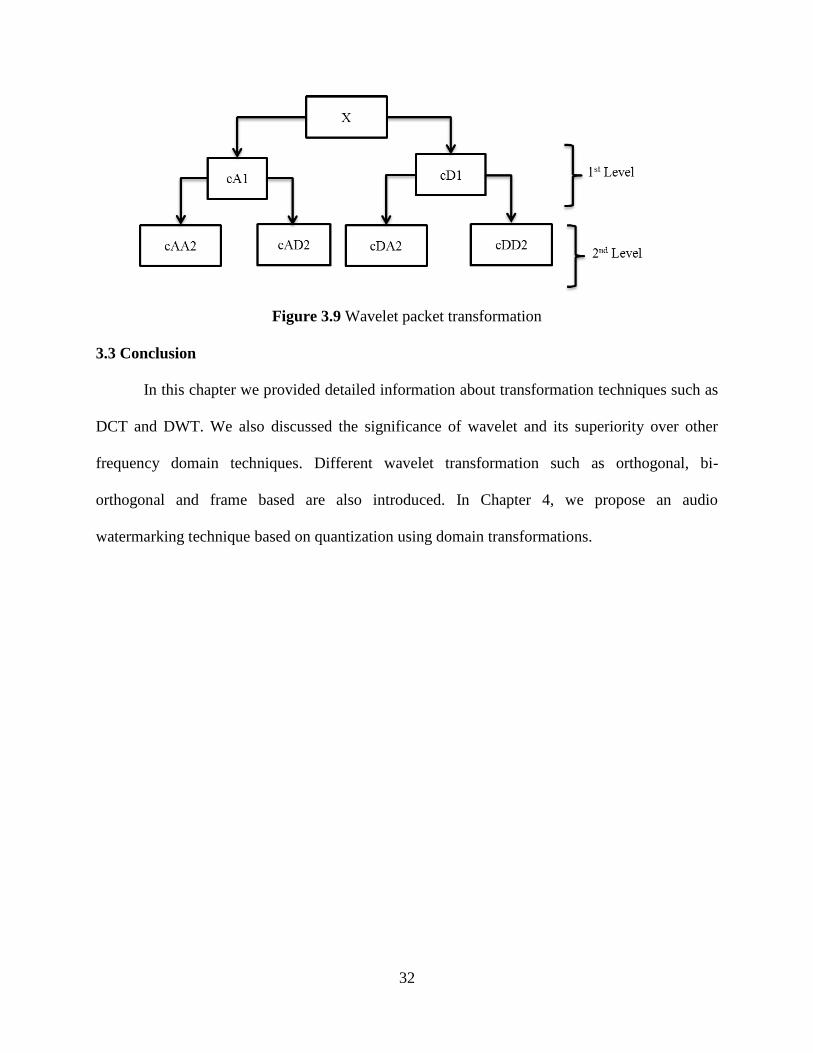
32
Figure 3.9 Wavelet packet transformation
3.3 Conclusion
In this chapter we provided detailed information about transformation techniques such as
DCT and DWT. We also discussed the significance of wavelet and its superiority over other
frequency domain techniques. Different wavelet transformation such as orthogonal, bi-
orthogonal and frame based are also introduced. In Chapter 4, we propose an audio
watermarking technique based on quantization using domain transformations.
33
4. PROPOSED TECHNIQUE FOR WATERMARKING
This chapter describes encryption techniques and principle of quantization [32]. We also
propose an audio watermarking algorithm using encryption techniques, domain transformation
and principle of quantization.
4.1 Encryption Techniques
The watermark to be embedded can be extracted if the embedding procedure is known.
However, it is important that the watermark is encrypted before embedding by which it will
become nearly impossible for the hackers to remove the watermark. Another important thing in
watermark embedding is that the energy of the watermark is evenly distributed throughout the
host signal. Else, the embedded signal seems like it has more noise embedded in it. Some of the
encryption techniques we used in this thesis are linear feedback shift register and Arnold
transform [2] [6].
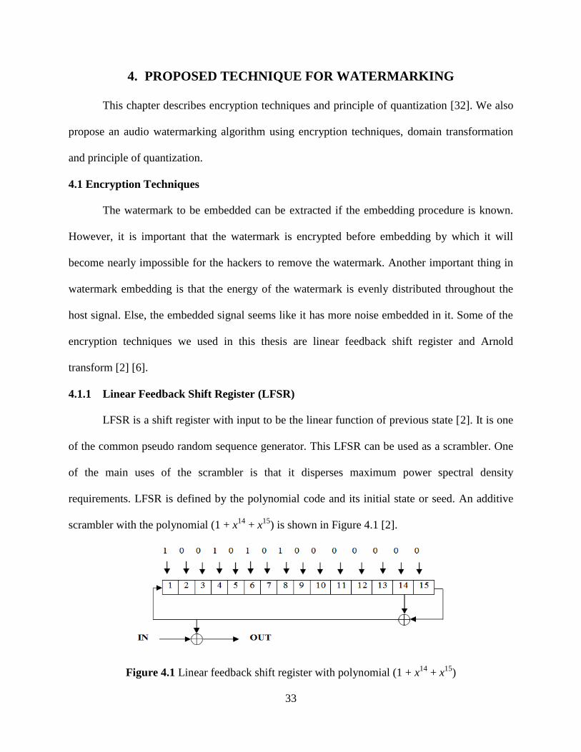
4.1.1 Linear Feedback Shift Register (LFSR)
LFSR is a shift register with input to be the linear function of previous state [2]. It is one
of the common pseudo random sequence generator. This LFSR can be used as a scrambler. One
of the main uses of the scrambler is that it disperses maximum power spectral density
requirements. LFSR is defined by the polynomial code and its initial state or seed. An additive
scrambler with the polynomial (1 + x14
+ x15
) is shown in Figure 4.1 [2].
Figure 4.1 Linear feedback shift register with polynomial (1 + x14
+ x15
)
34
4.1.2 Arnold Transform
An encryption technique, which is common in 2-dimensional domain, is Arnold transform
[6]. It is an image transformation technique used to scatter the pixels of the image. Due to the
periodicity of the transform, the image can be recovered from the transform domain information.
Let ,T
a b be the coordinate of the image pixel coordinate and ,T
a b be the coordinates after
the transform action. The size of the image is Nl×Nl Arnold transform is then expressed as
1 1
mod 1 2
l
a aN
b b
For encrypting 1-dimensional signal we should convert the 1-d data to a corresponding 2-
d data and then apply the transform, defined above. Arnold transform is a periodic
transformation. This makes it a good technique for retrieval. The process of obtaining the
original image using the transformed image is termed as Inverse Arnold Transform. Inverse
Arnold transform is obtained by using the equation below. Here 1 1,T
a b is the coordinate of the
Arnold transformed image pixel coordinates and 1 1,T
a b is the original pixel coordinates.
Mathematically,
1 1
1 1
2 1mod
1 1l
a aN
b b
Here 2 1
1 1
is the inverse of1 1
1 2
, where1 1
11 2
.
4.2 Quantization
Quantization is a technique used to approximate a real value to a relatively finite value. In
other words, a real value like 9.34 can be approximated to 9 or 10; by which it becomes easy for
analysis. Quantization can also be applied to a range of values say low or high. We can represent
35
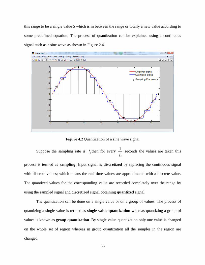
this range to be a single value S which is in between the range or totally a new value according to
some predefined equation. The process of quantization can be explained using a continuous
signal such as a sine wave as shown in Figure 2.4.
Figure 4.2 Quantization of a sine wave signal
Suppose the sampling rate is sf then for every 1
sf seconds the values are taken this
process is termed as sampling. Input signal is discretized by replacing the continuous signal
with discrete values; which means the real time values are approximated with a discrete value.
The quantized values for the corresponding value are recorded completely over the range by
using the sampled signal and discretized signal obtaining quantized signal.
The quantization can be done on a single value or on a group of values. The process of
quantizing a single value is termed as single value quantization whereas quantizing a group of
values is known as group quantization. By single value quantization only one value is changed
on the whole set of region whereas in group quantization all the samples in the region are
changed.
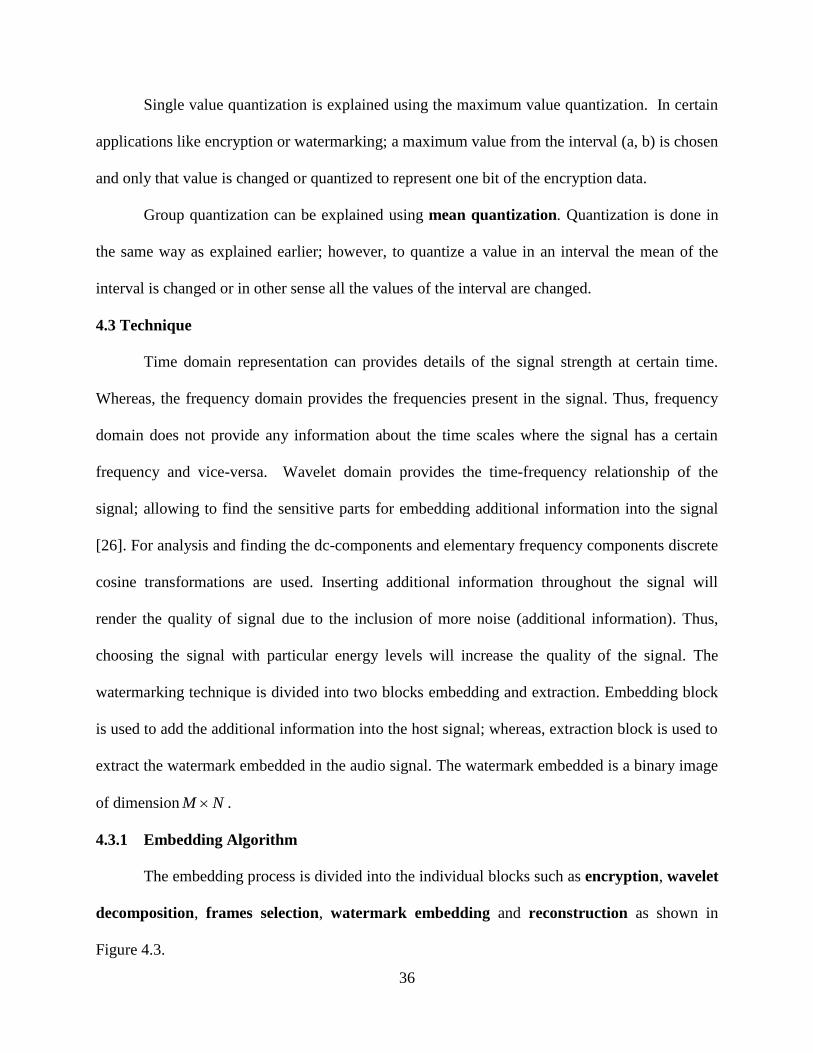
36
Single value quantization is explained using the maximum value quantization. In certain
applications like encryption or watermarking; a maximum value from the interval (a, b) is chosen
and only that value is changed or quantized to represent one bit of the encryption data.
Group quantization can be explained using mean quantization. Quantization is done in
the same way as explained earlier; however, to quantize a value in an interval the mean of the
interval is changed or in other sense all the values of the interval are changed.
4.3 Technique
Time domain representation can provides details of the signal strength at certain time.
Whereas, the frequency domain provides the frequencies present in the signal. Thus, frequency
domain does not provide any information about the time scales where the signal has a certain
frequency and vice-versa. Wavelet domain provides the time-frequency relationship of the
signal; allowing to find the sensitive parts for embedding additional information into the signal
[26]. For analysis and finding the dc-components and elementary frequency components discrete
cosine transformations are used. Inserting additional information throughout the signal will
render the quality of signal due to the inclusion of more noise (additional information). Thus,
choosing the signal with particular energy levels will increase the quality of the signal. The
watermarking technique is divided into two blocks embedding and extraction. Embedding block
is used to add the additional information into the host signal; whereas, extraction block is used to
extract the watermark embedded in the audio signal. The watermark embedded is a binary image
of dimension NM .
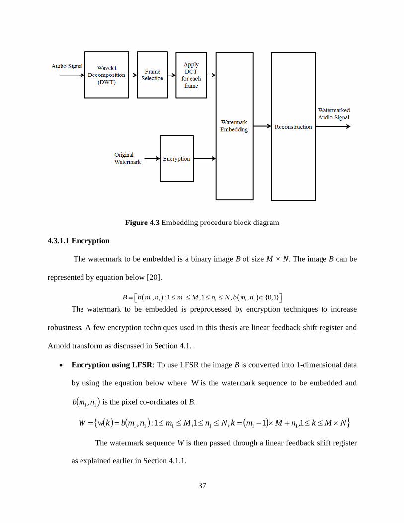
4.3.1 Embedding Algorithm
The embedding process is divided into the individual blocks such as encryption, wavelet
decomposition, frames selection, watermark embedding and reconstruction as shown in
Figure 4.3.
37
Figure 4.3 Embedding procedure block diagram
4.3.1.1 Encryption
The watermark to be embedded is a binary image B of size M × N. The image B can be
represented by equation below [20].
1 1 1 1 1 1, :1 ,1 , , {0,1}B b m n m M n N b m n
The watermark to be embedded is preprocessed by encryption techniques to increase
robustness. A few encryption techniques used in this thesis are linear feedback shift register and
Arnold transform as discussed in Section 4.1.
Encryption using LFSR: To use LFSR the image B is converted into 1-dimensional data
by using the equation below where W is the watermark sequence to be embedded and
11,nmb is the pixel co-ordinates of B.
NMknMmkNnMmnmbkwW 1,1,1,1:, 111111
The watermark sequence W is then passed through a linear feedback shift register
as explained earlier in Section 4.1.1.
38
Encryption using Arnold transform: To use Arnold transform, the two dimensional
image B is first processed using Arnold transformation thus obtaining B as explained in
Section 4.1.2. Obtained image is converted into a 1-d sequence by using transformation
equation below where W is the watermark sequence to be embedded and 11,nmb is the
pixel co-ordinates of B .
1 1 1 1 1 1, :1 ,1 , 1 ,1W w k b m n m M n N k m M n k M N
4.3.1.2 Wave Decomposition
Audio signal is decomposed into appropriate wavelet basis. Select the low frequency
coefficients of the decomposed signal i.e. iA where „i‟ is the level of decomposition. These
selected coefficients are made into non-overlapping frames of 128 in F using the equation below.
Note that the remaining coefficients at different levels are unaltered.
, :1 ,1 128, 128* 1 1,1 128i iF f p q A j p Length A q j p j
4.3.1.3 Frames Selection
The frames thus created are queued based on the energies of the frames. Then select the
first M × N frames for embedding in frame_selected.
4.3.1.4 Embedding Watermark
DCT is applied to all the frames in the frame_selected obtaining E. The watermark is
embedded in the dc-component or the 4th
ac-component of each frame in E depending on
whether the frame is even numbered or odd respectively. In other sense, if the frame number is
even then the embedding location is dc-component and if odd then chooses 4th
ac-component.
The equation below provides the quantization function used for embedding of watermark
where )( fvalue dc-component is or 4th
ac-component and Q is the quantization parameter.
39
( ) 10;
2
( ) 11;
2
value fif is even
QQuant value f
value fif is odd
Q
The quantization process is done by following the process below:
If Quant value f w f then No modifications are made
If Quant value f w f and ( )value f
Quant value fQ
then new mean is
obtained by
( ) 1
12
value fnewvalue f Q
Q
Else if Quant value f w f and ( )value f
Quant value fQ
then the new
mean is obtained by
( ) 1
12
value fnewvalue f Q
Q
Watermark is embedded uses mean quantization principle as the dc-component
resembles the mean of the signal. The concept of changing mean is to change every
sample in that frame.
4.3.1.5 Reconstruction
Inverse discrete cosine transformation (IDCT) is applied on the modified coefficients
for each frame. All the frames are reconstructed into one-dimensional continuous sequence in E.
Then obtained sequence is used in the reconstruction process. The inverse process of wavelet
decomposition is known as inverse discrete wavelets transform. The IDWT is applied taking the
modified low frequency coefficients i.e., E, and the untouched remaining components of i levels.
40
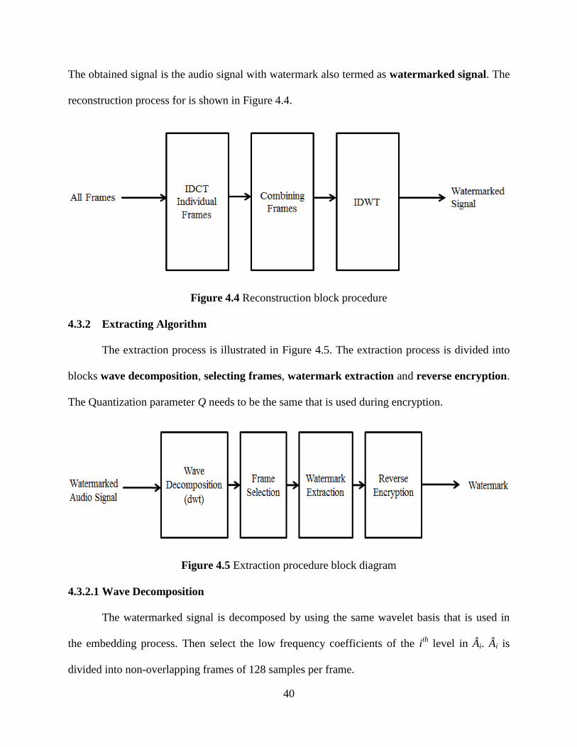
The obtained signal is the audio signal with watermark also termed as watermarked signal. The
reconstruction process for is shown in Figure 4.4.
Figure 4.4 Reconstruction block procedure
4.3.2 Extracting Algorithm
The extraction process is illustrated in Figure 4.5. The extraction process is divided into
blocks wave decomposition, selecting frames, watermark extraction and reverse encryption.
The Quantization parameter Q needs to be the same that is used during encryption.
Figure 4.5 Extraction procedure block diagram
4.3.2.1 Wave Decomposition
The watermarked signal is decomposed by using the same wavelet basis that is used in
the embedding process. Then select the low frequency coefficients of the ith
level in Âi. Âi is
divided into non-overlapping frames of 128 samples per frame.
41
4.3.2.2 Frames Selection
The frames thus created are queued based on the energies of the frames. Then select the
first M × N frames for extraction process in frame_selected.
4.3.2.3 Watermark Extraction
DCT is applied to all the frames in the frame_selected obtaining E . The watermark is
embedded in the dc-component of each frame or the 4th
ac-component of each frame
in Edepending on the weather frame number is even or odd respectively. The equation below
provides the quantization function used for embedding of watermark where ( )value f are dc-
component or 4th
ac-component.
( ) 10;
2
( ) 11;
2
value fif is even
QW f Quant value f
value fif is odd
Q
4.3.2.4 Reverse Encryption
From the previous step we get a one-dimensional sequence and need to be converted into
a two-dimensional image. The reverse encryption process need to be followed correspondingly
i.e., use inverse Arnold Transform and descrambler to extract the watermark. The 1-dimensional
sequence is converted into 2-dimensional image by using equation below.
1 1 1 1 1 1, :1 ,1 , 1 ,1W w m n W f m M n N f m M n f M N
Proper decryption techniques are used based on the chosen encryption techniques as
explained in Section 4.1.
4.4 Discussion
The watermarking technique uses the HAS properties of human ear and embeds the
watermark in the low frequency components of the audio signal obtaining high robustness and
less quality degradation. For redundancy the watermark is also embedded in the 4th
ac-
42
component in case of strong low pass filters. Highest level of decomposition is preferred based
on the availability of the length of the signal. The quantization parameter Q plays the major role
in the efficiency of the algorithm. Using of encryption techniques increases the robustness of the
technique.
The proposed technique is employed on an audio signal and its basic working is
evaluated. The embedded watermark is a 64×64 binary image. The quantization parameter Q
taken is 0.01 and the wavelet filter chosen is Daubechies 4 filter with 3-level decomposition. The
obtained watermarked signal has the SNR of 51.04 dB (>20 dB) and the RMS error is 4.1023
10-4
. The original audio signal and watermarked audio signal are shown in Figure 4.6. From
figure it can be noted that the original signal and the watermarked signal are similar.
Embedded watermark and the extracted watermark are shown in Figure 4.7. From the
figure it is clear that the watermark embedded and extracted are similar.
Figure 4.6 Original audio signal and watermarked audio signal time response
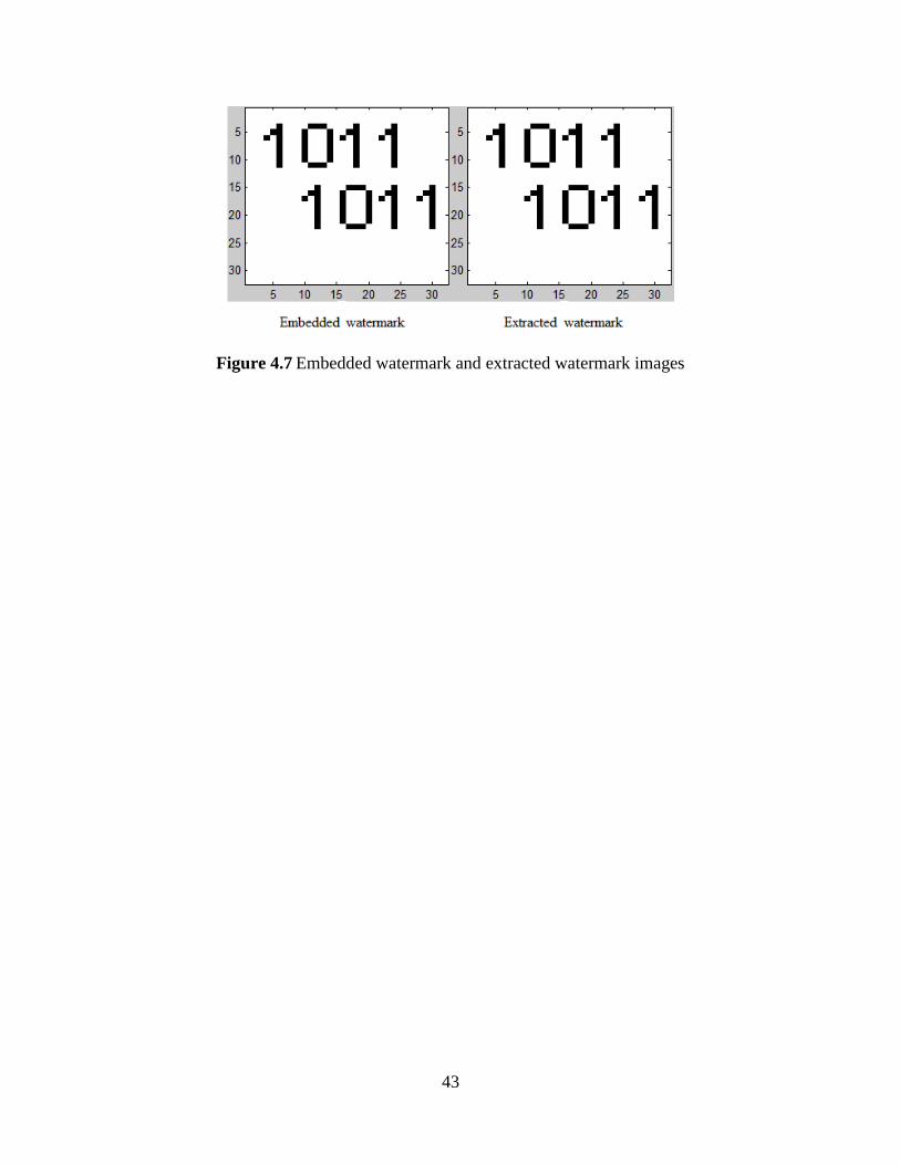
43
Figure 4.7 Embedded watermark and extracted watermark images
44
5. RESULTS AND DISCUSSION
In Chapter 4, we proposed an audio watermarking technique using domain
transformations. This chapter examines the performance of the proposed algorithm. It also
provides a performance comparison of the proposed algorithm vis-à-vis existing approaches. For
the purpose of performance evaluation, we have considered ALG1, ALG2, and ALG3, discussed
below. In all these methods the embedded watermark is a binary image of size 32×32 and the
audio samples considered are the same for efficient evaluation.
ALG-1: Bhat et al. have presented an algorithm for watermark embedding in DWT
domain using single value quantization [20]. The audio signal is divided into non-
overlapping frames of 2048 samples each. DWT is applied to each frame and the
maximum value in each frame is selected. The watermark bit is embedded by quantizing
the maximum values selected. The watermarked signal is obtained by applying IDWT for
each frame and reconstructing them.
ALG-2: Zhou et al. proposed an algorithm embedding watermark in 0th
DCT coefficient
and 4th
DCT coefficients [23]. In this approach the audio signal is transformed to
frequency domain using DCT. Transformed signal is then made into non-overlapping
frames of 8 samples each. Each bit of a watermark is embedded in separate frame by
using quantization principle. The procedure is continued for all the bits in the watermark.
The watermarked signal is obtained by applying IDCT for the modified samples.
ALG-3: Wu et al. uses DWT and self-synchronization concept to embed watermark [29].
In this procedure, a synchronization code is added to the watermark and then embedded
using the same procedure as in ALG-2. However, instead of embedding only watermark
only at one instance, they propose to embed multiple instances of the watermark with
synchronization code.

45
5.1 Performance Parameters
The performance parameters used for the performance are bit error rate (BER), signal to
noise ratio (SNR) and normalized co-relation (NC), discussed below.
Bit Error Rate
Bit error rate can be defined as the percentage of bits corrupted in the transmission of
digital information due to the effects of noise, interference and distortion. For example, the bits
to be transmitted are 11001100 and the received bits are 10000100. Comparing the number of
bits transmitted to received, two bits are affected by transmission. Hence, the BER in this
example is 2/8*100 = 25%.
Generally the BER of a binary image is computed using equation below. Where, Berr is
the number of error bits and NM refers to the size of the image (totaling the number of bits in
the image).
100%errBBER
M N
Signal to Noise Ratio
Signal to noise ratio is a parameter used to know the amount by which the signal is
corrupted by the noise. It is defined as the ratio of the signal power to the noise power.
Alternatively, it represents the ratio of desired signal (say a music file) to the background noise
level. SNR can be calculated by equation below.
Signal
Noise
PowerSNR
Power
Signal to noise ratio can also be calculated by equation below. Z is the un-watermarked
audio signal and Z' is the watermarked audio signal. Both Z and Z' has Mt samples.
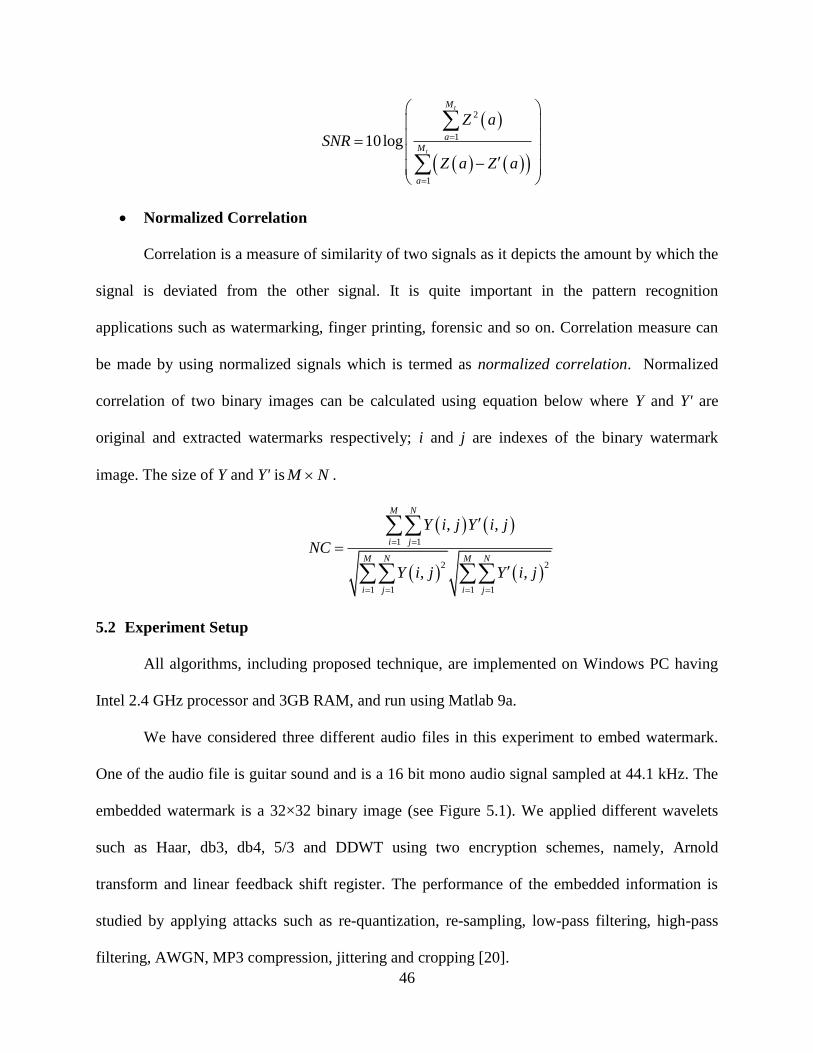
46
2
1
1
10log
t
t
M
a
M
a
Z a
SNR
Z a Z a
Normalized Correlation
Correlation is a measure of similarity of two signals as it depicts the amount by which the
signal is deviated from the other signal. It is quite important in the pattern recognition
applications such as watermarking, finger printing, forensic and so on. Correlation measure can
be made by using normalized signals which is termed as normalized correlation. Normalized
correlation of two binary images can be calculated using equation below where Y and Y' are
original and extracted watermarks respectively; i and j are indexes of the binary watermark
image. The size of Y and Y' is NM .
1 1
2 2
1 1 1 1
, ,
, ,
M N
i j
M N M N
i j i j
Y i j Y i j
NC
Y i j Y i j
5.2 Experiment Setup
All algorithms, including proposed technique, are implemented on Windows PC having
Intel 2.4 GHz processor and 3GB RAM, and run using Matlab 9a.
We have considered three different audio files in this experiment to embed watermark.
One of the audio file is guitar sound and is a 16 bit mono audio signal sampled at 44.1 kHz. The
embedded watermark is a 32×32 binary image (see Figure 5.1). We applied different wavelets
such as Haar, db3, db4, 5/3 and DDWT using two encryption schemes, namely, Arnold
transform and linear feedback shift register. The performance of the embedded information is
studied by applying attacks such as re-quantization, re-sampling, low-pass filtering, high-pass
filtering, AWGN, MP3 compression, jittering and cropping [20].

47
Figure 5.1 Watermark (Binary image)
For the complete analysis of the proposed technique different audio signals are
considered such as the guitar, classical, and music track. Figure 5.2 shows the time domain
response of these signals. Care has been taken to study the complete performance of the
algorithm by collecting diverge audio signals as shown in Figure 5.2. Same attacks are employed
on all audio signals. For appropriate analysis the audio watermarking techniques such as ALG-1,
ALG-2 and ALG-3 are implemented on the all considered audio signals.
Figure 5.2 Time domain response of the considered audio signals

48
5.3 Performance Analysis
The performance of the proposed algorithm against the signal processing and
desynchronized attacks such as re-quantization, re-sampling, jittering, mp3 compression, low
pass filtering, high pass filtering and the addition of Gaussian noise is evaluated. The wavelet
filter used for the analysis is Daubechies 4 wavelet with level 3 decomposition and the SNR of
the watermarked signal is 45 dB and Q = 0.05. The watermark taken is a 3232 size binary
image. From the observation, for SNR value of 45 dB the embedded watermark is inaudible to
the human ear. In addition to that, the NC and BER of the extracted watermark is nearly 1 and 0
for majority of the attacks, except MP3 compression.
Table 5-1 Performance evaluation of the embedded watermark with SNR of 45 dB
No
attack
Re-
quantization
Re-
sampling
AWGN
35 dB
Low
pass
filter
High
pass
filter
Cropping Jittering Mp3
NC 1 1 1 0.9973 1 1 1 1 0.97
BER 0 0 0 0.4882 0 0 0 0 5.467
Table 5-2 provides the comparison of performance of different algorithms when
undergone by signal processing and desynchronizing attacks. The performance parameter
considered is normalized correlation and SNR of the embedded signal is nearly 30dB for all the
considered algorithms. The watermark is the binary image of size 32×32. For the same SNR of
the watermarked signals the normalized correlation values are found when signal processing
attacks are employed. Normalized correlation values of 1 reflect the fact that extracted
watermark is more similar to the embedded watermark. From the observations all the other
techniques NC values are significantly less. Thus, robustness of the algorithm is high.
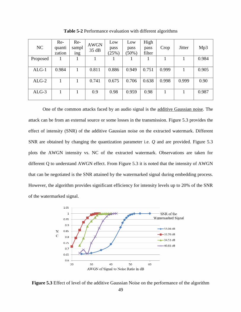
49
Table 5-2 Performance evaluation with different algorithms
NC
Re-
quanti
zation
Re-
sampl
ing
AWGN
35 dB
Low
pass
(25%)
Low
pass
(50%)
High
pass
filter
Crop Jitter Mp3
Proposed 1 1 1 1 1 1 1 1 0.984
ALG-1 0.984 1 0.811 0.886 0.949 0.751 0.999 1 0.905
ALG-2 1 1 0.741 0.675 0.706 0.638 0.998 0.999 0.90
ALG-3 1 1 0.9 0.98 0.959 0.98 1 1 0.987
One of the common attacks faced by an audio signal is the additive Gaussian noise. The
attack can be from an external source or some losses in the transmission. Figure 5.3 provides the
effect of intensity (SNR) of the additive Gaussian noise on the extracted watermark. Different
SNR are obtained by changing the quantization parameter i.e. Q and are provided. Figure 5.3
plots the AWGN intensity vs. NC of the extracted watermark. Observations are taken for
different Q to understand AWGN effect. From Figure 5.3 it is noted that the intensity of AWGN
that can be negotiated is the SNR attained by the watermarked signal during embedding process.
However, the algorithm provides significant efficiency for intensity levels up to 20% of the SNR
of the watermarked signal.
Figure 5.3 Effect of level of the additive Gaussian Noise on the performance of the algorithm

50
Using a wavelet filter gives an additional feature of decomposing to different levels
which gives the flexibility of capturing most significant (high energy) low frequency
components. The level of decomposition affects the imperceptibility property considerably.
Figure 5.4 provides the effect of levels of decomposition on the Signal to Noise Ratio of the
watermarked signal. The wavelet used is db4 with quantization parameter value of 0.015. From
Figure 5.4 it is noted that higher levels of decomposition provides higher SNR which makes
watermark inaudible. However, higher levels of decomposition lessen the number of components
available for embedding and that will make technique less robust. Hence, a 3 or 4-levels of
wavelet decomposition yields better performance.
Figure 5.4 Effect of level of decomposition of wavelet filter on signal to noise ratio
Effect of encryption techniques provide more robustness as the watermark embedding
sequence is scrambled. In addition to that, using of efficient scrambling techniques distributes
watermark evenly throughout the signal that increases SNR. Table 5-3 provides the effect of
SNR when encryption techniques are employed for Q = 0.05 for different wavelet filters. The
encryption techniques considered are Arnold Transform and linear feedback shift register. From
Table 5-3 it is noted that encryption techniques has least effect on SNR hence using of these
techniques will not make the watermark perceptible. However, the performance of the algorithm
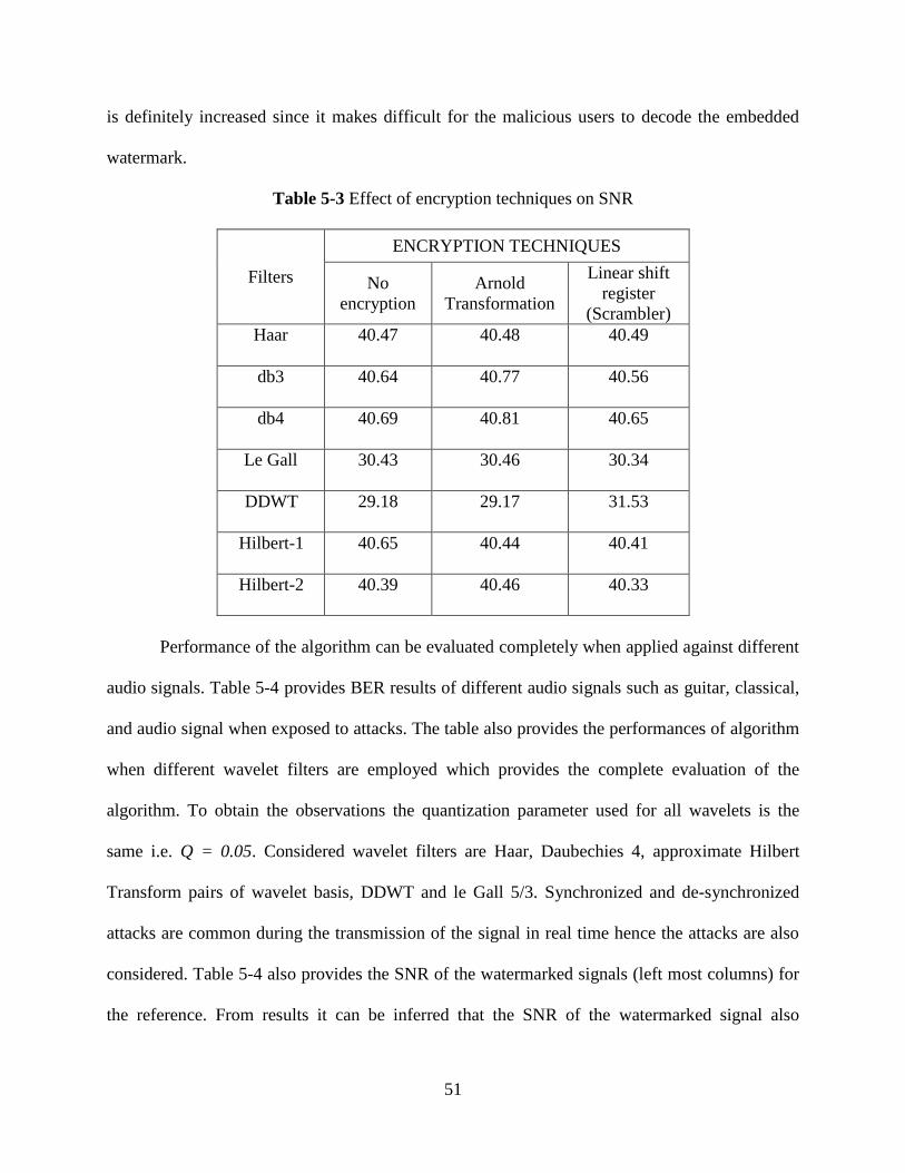
51
is definitely increased since it makes difficult for the malicious users to decode the embedded
watermark.
Table 5-3 Effect of encryption techniques on SNR
Filters
ENCRYPTION TECHNIQUES
No
encryption
Arnold
Transformation
Linear shift
register
(Scrambler)
Haar 40.47 40.48 40.49
db3 40.64 40.77 40.56
db4 40.69 40.81 40.65
Le Gall 30.43 30.46 30.34
DDWT 29.18 29.17 31.53
Hilbert-1 40.65 40.44 40.41
Hilbert-2 40.39 40.46 40.33
Performance of the algorithm can be evaluated completely when applied against different
audio signals. Table 5-4 provides BER results of different audio signals such as guitar, classical,
and audio signal when exposed to attacks. The table also provides the performances of algorithm
when different wavelet filters are employed which provides the complete evaluation of the
algorithm. To obtain the observations the quantization parameter used for all wavelets is the
same i.e. Q = 0.05. Considered wavelet filters are Haar, Daubechies 4, approximate Hilbert
Transform pairs of wavelet basis, DDWT and le Gall 5/3. Synchronized and de-synchronized
attacks are common during the transmission of the signal in real time hence the attacks are also
considered. Table 5-4 also provides the SNR of the watermarked signals (left most columns) for
the reference. From results it can be inferred that the SNR of the watermarked signal also

52
depends on the characteristics of the original signal. Here, for the same quantization parameter
guitar signal has least SNR compared to classical and album.
Table 5-4 BER of extracted attacks with different wavelet filters for different audio signals
Filter Types//
(Audio SNR) Types of attacks
Guitar
BER
Classical
BER
Album
BER
Re-quantization 0 0 0
Haar// Re-sampling 0 0 0
(Guitar 28.8dB) AWGN (40 dB) 0.683 11.23 1.757
(Classical 40.5 dB) Low pass filter 0 0.936 19.433
(Album 40.5dB) High pass filter 0 4.101 0
Cropping 0 0 0
Jittering 0 0 0
Re-quantization 0 0 0
db4// Re-sampling 0 0 0
(Guitar 28.6 dB) AWGN (40 dB) 1.464 1.269 0.9765
(Classical 40.8 dB) Low pass filter 0 9.181 19.23
(Album 40.5 dB) High pass filter 0 4.101 0
Cropping 0 0 0
Jittering 0 0 0
Re-quantization 0 0 0
Hilber-1// Re-sampling 0 0 0
(Guitar 28.86dB) AWGN (40 dB) 1.270 0.684 1.660
(Classical 40.44 dB) Low pass filter 0 11.03 18.85
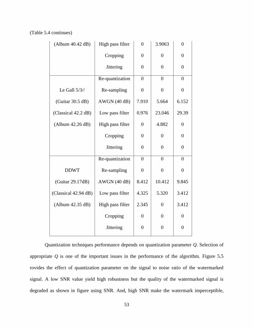
53
(Table 5.4 continues)
(Album 40.42 dB) High pass filter 0 3.9063 0
Cropping 0 0 0
Jittering 0 0 0
Re-quantization 0 0 0
Le Gall 5/3// Re-sampling 0 0 0
(Guitar 30.5 dB) AWGN (40 dB) 7.910 5.664 6.152
(Classical 42.2 dB) Low pass filter 0.976 23.046 29.39
(Album 42.26 dB) High pass filter 0 4.882 0
Cropping 0 0 0
Jittering 0 0 0
Re-quantization 0 0 0
DDWT Re-sampling 0 0 0
(Guitar 29.17dB) AWGN (40 dB) 8.412 10.412 9.845
(Classical 42.94 dB) Low pass filter 4.325 5.320 3.412
(Album 42.35 dB) High pass filter 2.345 0 3.412
Cropping 0 0 0
Jittering 0 0 0
Quantization techniques performance depends on quantization parameter Q. Selection of
appropriate Q is one of the important issues in the performance of the algorithm. Figure 5.5
rovides the effect of quantization parameter on the signal to noise ratio of the watermarked
signal. A low SNR value yield high robustness but the quality of the watermarked signal is
degraded as shown in figure using SNR. And, high SNR make the watermark imperceptible,
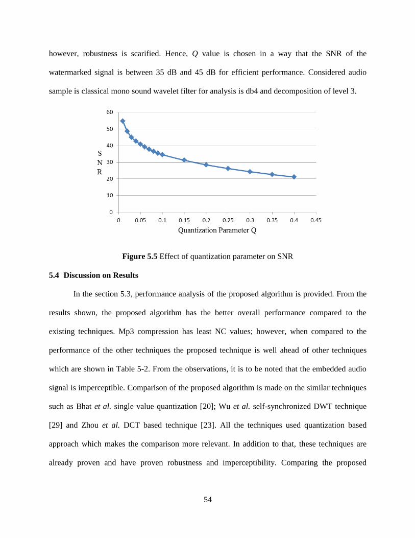
54
however, robustness is scarified. Hence, Q value is chosen in a way that the SNR of the
watermarked signal is between 35 dB and 45 dB for efficient performance. Considered audio
sample is classical mono sound wavelet filter for analysis is db4 and decomposition of level 3.
Figure 5.5 Effect of quantization parameter on SNR
5.4 Discussion on Results
In the section 5.3, performance analysis of the proposed algorithm is provided. From the
results shown, the proposed algorithm has the better overall performance compared to the
existing techniques. Mp3 compression has least NC values; however, when compared to the
performance of the other techniques the proposed technique is well ahead of other techniques
which are shown in Table 5-2. From the observations, it is to be noted that the embedded audio
signal is imperceptible. Comparison of the proposed algorithm is made on the similar techniques
such as Bhat et al. single value quantization [20]; Wu et al. self-synchronized DWT technique
[29] and Zhou et al. DCT based technique [23]. All the techniques used quantization based
approach which makes the comparison more relevant. In addition to that, these techniques are
already proven and have proven robustness and imperceptibility. Comparing the proposed
55
techniques performance with Bhat et al. algorithms performance it can be concluded that single
value quantization is less robust than mean value quantization.
Effect of different wavelet filters on the performance is provided and is noted that the
SNR and BER parameters are almost similar for Haar, db3, db4, and Hilbert wavelet filters.
However, using of le Gall and DDWT filters produces considerable results but is not as effective
as others. Arnold transform and linear feedback shift register can be used as the encryption
techniques to increase robustness against attackers intending to remove watermark. In addition to
that, quantization parameter need to be chosen based on the requirement of the usage of
technique. Low quantization value is chosen for high imperceptibility and high value for high
robustness. Additive Gaussian noise attack can be eliminated based on choosing the required
SNR which is achieved by Q.

56
6. CONCLUSION AND FUTURE WORK
This thesis proposes a new algorithm taking features of Human Auditory System and
the signal processing theories. Proposed algorithm is based on quantization in DWT and DCT
domains while considering the more active components of the signal.
The performance of the algorithm is provided by evaluating the performance parameters
such as signal to noise ratio, normalized correlation, and bit error rate. In addition, the effects of
the quantization types such as single value quantization and mean quantization on these
components are provided. From the results it is inferred that single value quantization technique
is less robust than the mean quantization. The performance of the algorithm is improved by using
the self-synchronization codes in the embedding process. But, the SNR is increased due to the
addition of more noise in the host signal and is not the feature of an efficient watermarking
technique. The technique proposed by using only DCT transformation is not robust against
simple Low pass filtering.
Choosing proper quantization parameter and wavelet filters have considerable effect on
the performance of the algorithm. Different wavelet filters are considered to evaluate the
algorithm performance completely. The orthogonal filters produce better performance over the
bi-orthogonal filters. Also, the level of decomposition of the wavelet filters has the effect on the
performance. Higher level of decomposition produces high SNR and loose robustness. From
studies level 3 produces better results bringing a tradeoff between SNR and robustness. In
addition, the effect of quantization parameter on the performance of the algorithm is also
examined. From results, it is noted that the higher value for quantization parameter will yield
high robustness and the watermark is easily perceivable. In contrary, choosing low quantization
parameter value makes the watermark unperceivable; however, the robustness of the algorithm is
degraded. From the experimental results it is noted that, quantization parameter value is chosen
57
in a way that the SNR of the embedded signal is between 35 dB and 45 dB and the wavelets filter
as db4 with level 3 for optimum results. It is noted that the proposed technique has better
performance than the already existing contemporary techniques.
The audio watermarking is relatively new and has wide scope for research. This thesis is
limited to binary image embedding and can be continued to gray scale images. The technique can
be implemented on live signals rather than a fixed signal as considered in this thesis. Some of
the real time audio signals include speech and conversation of pilot with ground controllers.
Further research can be carried on embedding watermark in video sequences i.e. movies or
surveillance. Applying watermarking technique on the surveillance system will decrease the
security issues by keeping track of the voice communication. One other application that can be
targeted is the watermarking of the live objects such as a person taking his tone and image. The
research can be extended by developing watermarking technique using neural networks.
58
REFERENCES
1. N.F. Johnson, S. Jajodia, and Z. Duric, Information hiding: Steganography and
watermarking attacks and countermeasures, Kluwer academic Publishers, 2000.
2. M. Goresky, A. M. Klapper, Fibonacci, and Galois, “Representations of Feedback-With-
Carry Shift Registers,” IEEE Transaction on Information Theory, Vol. 48, No. 11, pp.
2826-2836. 2002.
3. C. Shoemaker, “Hidden bits: A survey of techniques for digital watermarking,”
Independent study, EER 290, spring 2002.
4. B. Dumitrescu, and A. B. Rad, “A Method for Designing the Double-Density Dual-Tree
Discrete Wavelet Transform,” Proc. Int. TICSP Workshop on Local and Non-Local
Approximation in Image Processing, Lausanne, Switzerland, Aug. 2008.
5. S. Katzenbeisser, and F.A.P. Petitcolas, Information hiding techniques for
steganography and digital watermarking, Artech House Publishers, 2000.
6. G. Voyatzis, and I. Pitas, “Applications of toral automorphisms in image watermarking,”
Proceedings of International Conference on Image Processing, vol. 1, pp. 237– 240,
1996.
7. S.A. Craver, B. Liu, and M. Wu, “What can we reasonably expect from watermarks?
Applications of Signal Processing to Audio and Acoustics.” IEEE Workshop on
10/21/2001 -10/24/2001, pp. 223-226, 2001.
8. J. Bloom, I. Cox, T. Kalker, J. Linnartz, M. Miller, and C. Traw. “Copy protection for
DVD video,” Proceedings of the IEEE, vo. 7, Issue 87, pp. 1267- 1276, 1999.
9. F.A.P Petitcolas. “Watermarking schemes evaluation,” IEEE Signal Processing Magazine
[Online], Volume 17, Issue 5, pp.58-64, 2000.
10. SDMI. Call for Proposals for Phase II Screening Technology Version 1.0, 2000.
[Online]. Available: http://www.sdmi.org/download/FRWG00033102-AMD1.htm
[Accessed July 15. 2010].
11. M. Steinebach, F. Petitcolas, F. Raynal, J. Dittmann, C. Fontaine, S. Seibel, et al.,
“Stirmark benchmark: Audio watermarking attacks,” Proceedings of the International
Conference on Information Technology: Coding and Computing, pp. 49-54, 2001, Las
Vegas, Nevada.
12. X. Wang, and H. Zhao, “A Blind Audio Watermarking Robust Against Synchronization
Attacks,” CIS 2005, Part II, LNAI 3802, pp. 617-622, 2005.
13. E. Zwicker, and H. Fastl , Psychoacoustics. Springer Verlag, Berlin, Germany, 1999.
14. X. Wang , P. Niu, and H. Yang, “A robust digital audio watermarking based on statistics
charecteristics,” Elsevier Ltd., Pattern Recognition, vol. 42 pp. 3057-3064, 2009.
59
15. M. Navneet Kumar, “Watermarking Using Decimal Sequences,” M.S. thesis, Louisiana
State University, Baton Rouge, LA, USA, 2004.
16. N. Shaik Ashfaq, “Improved Watermarking Scheme Using Decimal Sequences,” M.S.
thesis, Louisiana State University, Baton Rouge, LA, USA, 2005.
17. W. Bender , D. Gruhl, and N. Morimoto, “Techniques for data hiding,” in IBM Systems
Journal, vol. 35(3), pp, 313-336.1996.
18. C. Nedeljko , “Algorithms For Audio Watermarking And Steganography”, Academic
Dissertation, University of Oulu, public discussion in Kuusamonsali (Auditorium
YB210), Linnanmaa, Finland, 2004.
19. S. Katzenbeisser, and F. A. P. Petitcolas, Information Hiding Techniques for
Steganography and Digital Watermarking, Artech House, Inc. 2000.
20. V. K. Bhat, I. Sengupta, and A. Das, “Audio Watermarking Based on Quantization in
Wavelet Domain,” ICISS 2008, LNCS 5352, pp. 235 -242, 2008.
21. M. Arnold, M. Schmucker, and S. D. Wolthusen, Techniques and Applications of Digital
Watermarking and Content Protection. Boston, London: Artech House, INC, 2003.
22. T. Todorov, “Spread Spectrum Watermarking Technique For Information System
Securing,” International Journal "Information Theories & Applications", Vol.11, pp. 405-
408. 2004.
23. Z. Zhiping, and Z. Lihau, “A Novel Algorithm for Robust Audio Watermarking Based on
Quantification DCT Domain,” Third International Conference on International
Information Hiding and Multimedia Signal Processing, vol. 1, pp. 441-444, 2007.
24. J. Y. Wang, M.S. Lai, K.W. Liang, and P.C. Chang, "Adaptive Wavelet Quantization
Index Modulation Technique for Audio Watermarking," International Computer
symposium(ICS) on Multimedia Technologies, Taipei, Taiwan, Dec. 2006.
25. A. B. Watson, “Image Compression Using the Discrete Cosine Transform,”
Mathematical Journal , vol. 4(1), pp. 81-88, 1994.
26. R. Polikar, "Home page - Dr. Robi Polikar," Jan 2001. [Online]. Available:
http://users.rowan.edu/~polikar/WAVELETS/WTtutorial.html. Accessed: July 21, 2010.
27. J. Kennedy, “IFPI Digital Music Report,” Jan. 21, 2010. [Online]. Available:
http://www.ifpi.org/content/library/DMR2010.pdf. Accessed: Aug 8, 2010.
28. S. Ali Khayam, “The Discrete Cosine Transform (DCT): Theory and Application,”
Information Theory and Coding, Seminar 1 – The Discrete Cosine Transform: Theory
and Application, March 10, 2003.
29. S. Wu, J. Huang, D. Huang and Y. Q. Shi, “A Self-Synchronized Audio Watermarking in
DWT Domain,” ISCAS 2004, vol. V, pp. 712-715, 2004.
60
30. W. Lanxun, Y. Chao, and P. Jiao, “An audio watermark embedding algorithm based on
mean-quantization in wavelet domains,” 8th Int. Conf. on Electronic Measurement and
Instruments, pp. 423–425, 2007.
31. K. Hofbauer, and H. Hering, “Noise Robust Speech Watermarking with Bit
Synchronisation for the Aeronautical Radio,” LNCS 4567, Springger-Verlag Berlin
Heidelberg, pp. 252-266, 2007.
32. R. Rajkiran and Suresh Rai, “A Robust Audio Watermarking Algorithm Based on
Statistical Characteristics and DWT+DCT Transforms,” 6th
International Conference on
Wireless Communications Networking and Mobile Computing, 2010.
33. I. W. Selesnick, “Symmetric Wavelet Tight Frames with Two Generators,” Applied and
Computational Harmonic Analysis, vol. 17(2), pp. 211-225, 2004.
34. I. W. Selesnick, “The Design of Approximate Hilbert Transform Pairs of Wavelet
Bases,” IEEE Trans. Of Signal Processing, vol. 50, no. 5, May 2002.
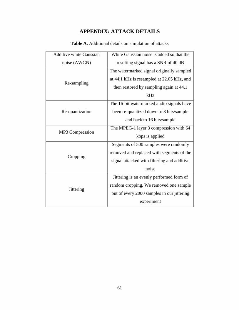
61
APPENDIX: ATTACK DETAILS
Table A. Additional details on simulation of attacks
Additive white Gaussian
noise (AWGN)
White Gaussian noise is added so that the
resulting signal has a SNR of 40 dB
Re-sampling
The watermarked signal originally sampled
at 44.1 kHz is resampled at 22.05 kHz, and
then restored by sampling again at 44.1
kHz
Re-quantization
The 16-bit watermarked audio signals have
been re-quantized down to 8 bits/sample
and back to 16 bits/sample
MP3 Compression The MPEG-1 layer 3 compression with 64
kbps is applied
Cropping
Segments of 500 samples were randomly
removed and replaced with segments of the
signal attacked with filtering and additive
noise
Jittering
Jittering is an evenly performed form of
random cropping. We removed one sample
out of every 2000 samples in our jittering
experiment
62
VITA
Rajkiran Ravula was born in Andhra Pradesh, in August 1986, India. He earned his
primary and secondary education from Word & Deed School in Hyderabad, Andhra Pradesh.
After finishing his high school, he took a very competitive entrance examination for engineering
known as EAMCET and stood in top 0.5%. After qualifying this examination he got admission
to Department of Electrical and Electronics Engineering degree, Chaitanya Bharathi Institute of
Technology one of the prestigious institutes in Andhra Pradesh, India. He received his Electrical
and Electronics Engineering from Osmania University, Hyderabad, India, in spring 2008. After
his graduation, he joined Medha Servo Drives pvt. Ltd., India, where he served as design
engineer in Control Electronics Department. After working for one and half year he came to
United States of America to pursue master‟s degree. He then joined the graduate program at
Louisiana State University, Baton Rouge, in January 2008. He is a candidate for the degree of
Master of Science in Electrical Engineering to be awarded at the commencement of fall, 2010.
Top Related